Abstract

We propose a Bayesian nonparametric model based on Markov Chain Monte Carlo (MCMC) methods for the joint reconstruction and prediction of discrete time stochastic dynamical systems, based on $m$-multiple time-series data, perturbed by additive dynamical noise. We introduce the Pairwise Dependent Geometric Stick-Breaking Reconstruction (PD-GSBR) model, which relies on the construction of a $m$-variate nonparametric prior over the space of densities supported over $\mathbb{R}^{m}$. We are focusing in the case where at least one of the time-series has a sufficiently large sample size representation for an independent and accurate Geometric Stick-Breaking estimation, as defined in Merkatas et al. (2017). Our contention, is that whenever the dynamical error processes perturbing the underlying dynamical systems share common characteristics, underrepresented data sets can benefit in terms of model estimation accuracy. The PD-GSBR estimation and prediction procedure is demonstrated specifically in the case of maps with polynomial nonlinearities of an arbitrary degree. Simulations based on synthetic time-series are presented.

Keywords: Bayesian nonparametric inference; Mixture of Dirichlet process; Geometric Stick-Breaking weights; Random dynamical systems; Chaotic dynamical systems

1 Introduction

The interdisciplinary framework of nonlinear dynamical systems, has been used extensively for the modeling of time varying phenomena in physics, chemistry, biology, economics and so forth, that they exhibit complex and irregular behavior (Ott, 2002). The apparently random and unpredictable behavior of deterministic chaotic dynamics, right from the early days of the theory, prompted to the use of random or probabilistic methods (Berliner, 1992; Chatterjee and Yilmaz, 1992). At the same time, the ubiquitous effect of the different kinds of noise in experimental or real data, reinforced the interaction between nonlinear dynamics and statistics (Mees, 2012).

When the nonlinear procedure is influenced by the uncertainty of the measurement process, the resulting time-series can be thought of as the corruption of the true system states by observational noise. We can consider the noise in this case, as being added after the time evolution of the trajectories under consideration, thus inducing a blurring effect on the true evolution of the process. In this case the dynamics of the process are not influenced, and the invariant measure of the process is the convolution of the unperturbed measure and the noise distribution. Observational noise corrupted dynamical systems are often confronted with time delay embedding techniques and related methods (Ruelle and Takens, 1971; Abarbanel, 2012; Kantz and Schreiber, 2004).

In the case of dynamical or interactive noise, the noise is incorporated at each step of time evolution of the trajectories. For example consider a situation in which at each discrete time, the state of the system is reached with some error. Then the constructed predictive model consists of two parts, the nonlinear-deterministic component and the random noise. In such cases where the noise acts as a driving force, the underlying deterministic dynamics can be drastically modified (Jaeger and Kantz, 1997), and the predictive model constitutes what is known as a random dynamical system (Arnold, 1998; Smith and Mees, 2000). From a modeling perspective, the existence of a stochastic forcing term can be thought of as representing the error in the assumed model, mimicking the aggregate action of variables not included in the model, compensating for a small number of degrees of freedom. In fact, when a small number of degrees of freedom is segregated from a larger coupled system, usually has as an outcome, reduced equations with deterministic and stochastic components (He and Habib, 2013).

Methods based on deterministic inference in the case of dynamical noise are inefficient, and many methods have been proposed by various researchers to address the various aspects of the problem. A theorem formulated to cope with the embedding problem for random dynamical systems is given in Muldoon et al. (1998). In Siegert, Friedrich, and Peinke (1998) and Siefert and Peinke (2004) the issue of dynamical reconstruction is addressed for stochastic systems described by Langevin type of equations under different types of random noise. Because of the different impact of the noise types, the goal of estimating the noise density directly from the data is highly significant (Heald and Stark, 2000; Strumik and Macek, 2008; Siefert et al., 2004).

The Bayesian framework (Robert, 2007) was initially put into context by Davies (Davies, 1998) for nonlinear noise reduction. Meyer and Christensen (2000, 2001) applied MCMC methods for the parametric estimation of state-space nonlinear models, extending maximum likelihood-based methods (McSharry and Smith, 1999). Later, Smelyanskiy et al. (2005) reconstructed stochastic nonlinear dynamical models from trajectory measurements, using path integral representations for the likelihood function, extended for nonstationary systems in Luchinsky et al. (2008). Matsumoto et al. (2001) introduced a hierarchical Bayesian approach and later, Nakada et al. (2005) applied a hybrid Monte Carlo scheme for the reconstruction and prediction of nonlinear dynamical systems. More recently in Molkov et al. (2012), a Bayesian technique was proposed for predicting the qualitative behavior of random dynamical systems from time-series.

In the literature of stochastically perturbed dynamical systems, error processes are frequently modeled via zero mean Gaussian distributions. Such an assumption, when violated, can cause inferential problems. For example when the noise process produces outlying errors the estimated variance under the normality assumption, is artificially enlarged causing poor inference for the system parameters. Alternatively, we could make the assumption of the existence of two sources of random perturbations. For example we could assume that an environmental source, caused perhaps by spatiotemporal inhomogeneities (Strumik and Macek, 2008), is producing weak and frequent perturbations. At the same time, stronger but less frequent perturbations in the form of outlying errors, are coming from a higher dimensional deterministic component. Other cases could include systems exerting noise at random time intervals and impulsive noise (Shinde and Gupta, 1974; Middleton, 1977). These are situations where the noise probability density function does not decay in the tails like a Gaussian. Also, when the system under consideration is coupled to multiple stochastic environments the driving noise term may exhibit non-Gaussian behavior, see for example references Kanazawa et al. (2015a) and Kanazawa et al. (2015b).

A number of approaches for modeling time-series in a Bayesian nonparametric context have been proposed in the literature. For example, an infinite mixture of time-series models has been proposed in Rodriguez and Ter Horst (2008). A Markov-switching finite mixture of independent Dirichlet process mixtures has been proposed by Taddy and Kottas (2009). More recently, Jensen and Maheu (2010) and Griffin (2010), considered Dirichlet process mixtures for stochastic volatility models in discrete and continuous time, respectively. An approach for continuous time-series modeling based on time dependent Geometric Stick-Breaking process mixtures can be found in Mena, Ruggiero, and Walker (2011). For a Bayesian nonparametric nonlinear noise reduction approach see Kaloudis and Hatjispyros (2018).

Recently there has been a growing research interest for Bayesian nonparametric modeling in the context of multiple time-series. In Fox et al. (2009) a Bayesian nonparametric model based on the Beta process was introduced in order to model dynamical behavior shared among a number of time-series. They represented the behavioral set with an attribute list encoded by an $n\times k$ binary matrix, with $n$ the number of time-series and $k$ the number of features. Their approach allowed for potentially an infinite number of behaviors $k$. This was an improvement of a similar approach of a previous work Fox et al. (2008) where the time-series shared exactly the same set of behaviors. In Nieto-Barajas and Quintana (2016), a Bayesian nonparametric dynamic autoregressive model for the analysis of multiple time-series was introduced. They considered an autoregressive model of order $p$ for each of the time-series in the collection, and a Bayesian nonparametric prior based on dependent Pólya trees. The dependent prior, with its median fixed at zero, was used for the modeling of the errors.

In a previous work Merkatas, Kaloudis, and Hatjispyros (2017) we have dealt with the problem of identifying the deterministic part of a stochastic dynamical system and the estimation of the associated unknown density of dynamical perturbations, which is perhaps non-Gaussian, simultaneously from data via Geometric Stick-Breaking (GSB) mixture processes. In this work we will attempt to generalize the so-called Geometric Stick-Breaking Reconstruction (GSBR) model under a multidimensional setting, in order to reconstruct and predict jointly, an arbitrary number of discrete time dynamical systems. More specifically, given a collection of $m$ noisy chaotic time-series, we propose a Bayesian nonparametric mixture model for the joint reconstruction and prediction of $m$ dynamical equations.

Our method of joint reconstruction and prediction, is primarily based on the existence of a multivariate Bayesian nonparametric prior over the collection of the unknown dynamical noise processes. It is based on the Pairwise Dependent Geometric Stick-Breaking Process mixture priors developed in Hatjispyros et al. (2017), under the following assumptions:

1. The dynamical equations have deterministic parts that they belong to known families of functions; for example they can be polynomial or rational functions.

2. A-priori we assume that we have the knowledge that the noise processes corrupting dynamically the observed multiple time-series, have possibly common characteristics; for example the error processes could reveal a similar tail behavior or (and) have common variances, or simply they come from the same noise process which is (perhaps) non-Gaussian.

Our contention is that whenever there is at least one sufficiently large data set, using borrowing of strength prior specifications, we will be able to recover the dynamical process for which we have insufficient information i.e. the process for which the sample size is inadequate for an independent GSBR reconstruction and prediction.

This paper is organized as follows. In Sec. II, we are giving some preliminary notions on the GSB mixture priors applied on a single discretized random dynamical system. In Sec. III, we introduce the joint probability model for the multiple time-series observations and we derive the PD-GSBR model. We describe the associated joint nonparametric likelihood for the model, and as a special case we derive the joint parametric likelihood corresponding to the assumption of common Gaussian noise along the multiple time-series observations. We also provide the PD-GSBR based Gibbs sampler for the estimation of the unknown error processes, the control parameters, the initial conditions, and the out-of-sample predictions. In Sec. IV, we resort to simulation. We apply the PD-GSBR model on the reconstruction and prediction of two pairs and one triple of random polynomial maps that are dynamically perturbed additively, by noise processes which are non-Gaussian. Finally, conclusions and directions for future research are discussed.

2 Preliminaries

For $j=1,\ldots,m$, we consider the following assemblage of the $m$ decoupled random recurrences

$$X_{ji} =T_{j}(\theta_{j},X_{j,i-1},\ldots,X_{j,i-\rho_{j}},Z_{ji})$$ (1)

$$=g_{j}(\theta_{j},X_{j,i-1},\ldots,X_{j,i-\rho_{j}})+Z_{ji},\,\,i\geq 1,$$

where $g_{j}:\Theta_{j}\times{\mathbb{X}}_{j}^{\rho_{j}}\to{\mathbb{X}}_{j}$, for some compact subsets ${\mathbb{X}}_{j}$ of $\mathbb{R}$, $(X_{ji})_{i\,\geq\,1-\rho_{j}}$ and $(Z_{ji})_{i\,\geq\,1}$ are real random variables over some probability space $(\Omega,{\cal F},{\rm P})$; we denote by $\theta_{j}\in\Theta_{j}\subseteq\mathbb{R}^{q_{j}}$ any dependence of the deterministic map $g_{j}$ on parameters. $g_{j}$ is a nonlinear map, for simplicity continuous in the variable ${\bf X}_{j,i:\rho_{j}}:=(X_{j,i-1},\ldots,X_{j,i-\rho_{j}})$. We assume that the random variables $Z_{ji}$ are independent to each other, and independent of the states $X_{j,i-r_{j}}$ for all $r_{j}<i+\rho_{j}$. In addition, we assume that the additive perturbations $Z_{ji}$ are identically distributed from zero mean symmetric distributions with unknown densities $f_{j}$ defined over the real line so that $T_{j}:\Theta_{j}\times{\mathbb{X}}_{j}^{\rho_{j}}\times\mathbb{R}\to\mathbb{R}$. Finally, notice that the lag-one stochastic process $(W_{ji}^{1},\ldots,W_{ji}^{\rho_{j}})$ formed out by the time-delayed values of the $(X_{ji})$ process is Markovian over $\mathbb{R}^{\rho_{j}}$.

We assume that there is no observational noise. We denote the set of observations along the $m$ time-series as ${\boldsymbol{x}}=\{x_{ji}:1\leq j\leq m,1\leq i\leq n_{j}\}$ and with ${\boldsymbol{x}}_{j}=\{x_{ji}:1\leq i\leq n_{j}\}$ the set of observations in the $j$-th time-series. These are realizations of the nonlinear stochastic processes defined in (1) for some unknown initial conditions ${\boldsymbol{x}}_{0}=\{{\boldsymbol{x}}_{j,1:\rho_{j}}:1\leq j\leq m\}$. The collection of the time-series observations $\boldsymbol{x}$, depends solely on the initial distribution of the variable ${\boldsymbol{X}}_{0}$, the values of the control parameters ${\boldsymbol{\theta}}=\{\theta_{j}:1\leq j\leq m\}$, and the particular realization of the noise processes.

In Merkatas, Kaloudis, and Hatjispyros (2017) a Bayesian nonparametric methodology is proposed for the estimation and prediction of a single discretized random dynamical system from an observed noisy time-series of length $n$. It relaxes the assumption of normal perturbations by assuming that the prior over the unknown density $f$ of the additive dynamical errors, is a random infinite mixture of zero mean Gaussian kernels. More specifically a-priori we set

$$f(z)=\int_{v>0}{\cal N}(z|0,v^{-1})\,\mathbb{G}(dv)=\sum_{k=1}^{\infty}\pi_{k}\,{\cal N}(z|0,\tau_{k}^{-1}),$$

where $\mathbb{G}$ is a GSB random measure. The random measure $\mathbb{G}$ is closely related to the well known Dirichlet random measure $\mathbb{G}^{\prime}=\sum_{k\geq 1}w_{k}\delta_{\tau_{k}}\sim{\cal DP}(c,G_{0})$(Ferguson, 1973; Sethuraman, 1994). $\delta_{\tau_{k}}$’s are Dirac measures concentrated on the random precisions $\tau_{k}$’s, which in turn are independently drawn (i.i.d.) from the mean parametric distribution $G_{0}$, being the prior guess of $\mathbb{G}^{\prime}$ i.e. $\mathbb{E}(G^{\prime}(A))=G_{0}$ for measurable subsets $A$ of $\mathbb{R}_{+}$. The probability-weights $w_{k}$ are stick-breaking in the sense that $w_{1}=v_{1}$ and $w_{k}=v_{k}\prod_{l<k}(1-v_{l})$ and random because $v_{k}\stackrel{{\scriptstyle{\rm i.i.d.}}}{{\sim}}{\cal B}e(1,c)$ a beta density with mean $(1+c)^{-1}$. We define the GSB random measure as $\mathbb{G}=\sum_{k\geq 1}\pi_{k}\delta_{\tau_{k}}\sim{\cal GSB}(\alpha,\beta,G_{0})$ with $\pi_{k}=\mathbb{E}(w_{k})$, hence removing a hierarchy from the random measure $\mathbb{G}^{\prime}$(Fuentes-García, Mena, and Walker, 2010). Then for $\lambda=(1+c)^{-1}$, we have $\pi_{k}=\lambda\,(1-\lambda)^{k-1}$ and $\mathbb{E}(G(A))=G_{0}$. Finally we randomize the probability-weights by letting $\lambda\sim{\cal B}e(\alpha,\beta)$; then $\lambda$ a-posteriori is again beta with its parameters updated by a sufficient statistic of the data. In Merkatas, Kaloudis, and Hatjispyros (2017) it is shown that a $\mathbb{G}$-based Bayesian nonparametric framework for dynamical system estimation is efficient, faster and less complicated when compared to Bayesian nonparametric modeling via the Dirichlet process.

To sample from the posterior of $f(z)$, the control parameters of the deterministic part, the initial condition and the future observations, given the noisy time-series, in a finite number of steps we have to:

1. Introduce the infinite mixture allocation variables $\{d_{i}:1\leq i\leq n\}$, such that P$\{d_{i}=k\}=\pi_{k}$ for $k\geq 1$, indicating the component of the infinite mixture the $i$th observation came from.

2. Augment the random density $f(z)$, with the auxiliary variables $\{N_{i}:1\leq i\leq n\}$, such that the $N_{i}$’s are identically distributed from the specific negative binomial distribution $f_{N}(k|\lambda)={\cal NB}(k|2,\lambda)=k\lambda^{2}(1-\lambda)^{k-1}{\cal I}(k\geq 1)$. Then $d_{i}$ conditionally on $N_{i}$, attains the discrete uniform distribution over the random set $\{1,\ldots,N_{i}\}$.

Thereby, the dimension of the Gibbs sampler will be of order $\max_{1\leq i\leq n}N_{i}<\infty$.

3 The PD-GSBR model

We will model a-priori the errors $Z_{j}$ in the multiple recurrence relation (1) with a multivariate distribution over the space of densities. More specifically, we are interested in constructing for any finite integer $m\geq 2$

$${\boldsymbol{f}}=(f_{1},\ldots,f_{m})^{T},$$ (2)

where $T$ denotes transposition, each $f_{j}$ is a random density function, and we are able to understand the dependence mechanism between pairs $(f_{j},f_{l})$ for each $j\neq l$.

We will allow pairwise dependence between any two $f_{j}$ and $f_{l}$, so that there is a unique common component for each pair $(f_{j},f_{l})$. For example consider such a dependence structure for $m=3$ for the random variables $Y_{1}=M_{11}\!+\!M_{12}\!+\!M_{13}$, $Y_{2}=M_{12}\!+\!M_{22}\!+\!M_{23}$ and $Y_{3}=M_{13}+M_{23}+M_{33}$, where all the $M_{jl}$ random variables are mutually independent. Then the dependence between $Y_{j}$ and $Y_{l}$ is created via them having $M_{jl}$ in common and it is easy to show that Cov$(Y_{j},Y_{l})=$Var$(M_{jl})$. Therefore, the independent variables $M_{12},M_{13}$ and $M_{23}$ play the rôle of common parts for the pairs $(Y_{1},Y_{2}),(Y_{1},Y_{3})$ and $(Y_{2},Y_{3})$, respectively. On the other hand the independent variables $M_{11},M_{22}$ and $M_{33}$ serve as idiosyncratic parts of the variables $Y_{1},Y_{2}$ and $Y_{3}$, respectively. In a more compact notation, we set ${\boldsymbol{Y}}={\boldsymbol{M}}\!\cdot\!{\boldsymbol{1}}$ where ${\boldsymbol{Y}}$ is the column vector of $Y_{j}$’s, ${\boldsymbol{M}}$ is a random symmetric matrix of independent random variables, and $\boldsymbol{1}$ a $3\times 1$ matrix of ones.

We will use this basic plan but instead of the real valued random vector $\boldsymbol{Y}$, we have the vector of random density functions $\boldsymbol{f}$. We set ${\boldsymbol{f}}=({\boldsymbol{p}}\otimes{\boldsymbol{M}})\cdot{\boldsymbol{1}}$. In this case $\boldsymbol{M}$ is a $m\times m$ symmetric matrix of independent random zero mean mixture densities, $\boldsymbol{p}$ is a random stochastic matrix (its row elements add up to $1$ a.s.), and $\boldsymbol{1}$ a $m\times 1$ matrix of ones. The Hadamard product of the two matrices $\boldsymbol{p}$ and $\boldsymbol{M}$ is defined as $({\boldsymbol{p}}\otimes{\boldsymbol{M}})_{jl}=p_{jl}M_{jl}$, whence $f_{j}=\sum_{l=1}^{m}p_{jl}\,M_{jl}$ with $M_{jl}=M_{lj}$ and ${\rm Cov}(f_{j},f_{l}\,|\,{\boldsymbol{p}})=p_{jl}\,p_{lj}{\rm Var}(M_{jl})$. We will model the densities $f_{j}$ via

$$f_{j}(z)=\int\limits_{v>0}{\cal N}(z\,|\,0,v^{-1})\,\mathbb{Q}_{j}(dv),\,\,\mathbb{Q}_{j}=\sum_{l=1}^{m}p_{jl}\mathbb{G}_{jl}$$

$$\mathbb{G}_{jl}=\sum_{k=1}^{\infty}\pi_{jlk}\delta_{\tau_{jlk}}\stackrel{{\scriptstyle{\rm ind.}}}{{\sim}}{\cal GSB}(\alpha_{jl},\beta_{jl},G_{0}),\,\,\mathbb{G}_{jl}=\mathbb{G}_{lj}\,\,{\rm a.s.},$$

where for the random selection-probabilities $p_{jl}$ it is that $\sum_{l=1}^{m}p_{jl}=1$ a.s., and $\tau_{jlk}\stackrel{{\scriptstyle{\rm i.i.d.}}}{{\sim}}G_{0}$. The random probability-weights $\pi_{jlk}$ satisfy $\sum_{k\geq 1}\pi_{jlk}=1$ a.s. with

$$\pi_{jlk}=\lambda_{jl}\,(1-\lambda_{jl})^{k-1},\,\,\,k\geq 1.$$ (3)

The $\lambda_{jl}$’s are random geometric-probabilities with $\lambda_{jl}\stackrel{{\scriptstyle{\rm ind.}}}{{\sim}}{\cal B}e(\alpha_{jl},\beta_{jl})$ for fixed hyperparameters $\alpha_{jl}$ and $\beta_{jl}$. Then, the nonparametric prior over the $Z_{j}$ error in (1) attains the representation

$$f_{j}(z)=\sum_{l=1}^{m}p_{jl}\,M_{jl}(z),$$

where each $M_{jl}$ is an infinite mixture of normal zero mean kernels via the random mixing measure $\mathbb{G}_{jl}$ i.e.

$$M_{jl}(z)=\int_{v>0}{\cal N}(z|0,v^{-1})\,\mathbb{G}_{jl}(dv)=\sum_{k=1}^{\infty}\pi_{jlk}\,{\cal N}(z|0,\tau_{jlk}^{-1}).$$

Clearly, because $\mathbb{G}_{jl}=\mathbb{G}_{lj}$ it is that $M_{jl}=M_{lj}$.

We have the following:

1. The random infinite mixtures $\{M_{jl}:1\leq j<l\leq m\}$ a-posteriori given the observed time-series, will capture common characteristics among the pairs of noise densities $\{(f_{j},f_{l}):1\leq j<l\leq m\}$.

2. The mixtures $\{M_{jj}:1\leq j\leq m\}$ a-posteriori will be describing idiosyncratic characteristics of the noise densities $\{f_{j}:1\leq j\leq m\}$.

It follows that the model $({\boldsymbol{x}}|{\boldsymbol{x}}_{0})$ of the time-series observations conditional on the unknown initial conditions, in a hierarchical fashion, is given by

$$x_{ji}|\,{\boldsymbol{x}}_{j,i:\rho_{j}},\theta_{j},\tau_{ji}\stackrel{{\scriptstyle{\rm ind.}}}{{\sim}}{\cal N}(g_{j}(\theta_{j},{\boldsymbol{x}}_{j,i:\rho_{j}}),\tau_{ji}^{-1})$$ (4)

$$\qquad\qquad\text{where }\,\,1\leq i\leq n_{j},\,1\leq j\leq m$$

$$\tau_{ji}\,|\,\mathbb{Q}_{j}\stackrel{{\scriptstyle{\rm i.i.d.}}}{{\sim}}\mathbb{Q}_{j}$$

$$\mathbb{Q}_{j}=\sum_{l=1}^{m}p_{jl}\mathbb{G}_{jl},\,\,\sum_{l=1}^{m}p_{jl}=1,\,\,\ \mathbb{G}_{jl}=\mathbb{G}_{lj}\,\,{\rm a.s.}$$

$$\mathbb{G}_{jl}\stackrel{{\scriptstyle{\rm ind.}}}{{\sim}}{\cal GSB}(\alpha_{jl},\beta_{jl},G_{0}).$$

While our method for pairwise dependent joint reconstruction and prediction can be used for dynamical systems where each state $x_{ji}$ depends on the previous $\rho_{j}$ states ${\boldsymbol{x}}_{j,i:\rho_{j}}$, for simplicity and ease of exposition, in the sequel we will focus on the special case $\rho_{j}=1$ for all $j=1,\ldots,m$. Also, with ${\boldsymbol{x}}^{\prime}$ we will denote the future unobserved observations along the $m$ multiple time-series, and with ${\boldsymbol{x}}_{j}^{\prime}=(x_{j,n_{j}+1},\ldots,x_{j,n_{j}+T_{j}})$ the $T_{j}$ future unobserved observations of the $j$-th time-series.

3.1 The nonparametric posterior

Using Bayes’ theorem, it is that

$$\Pi({\boldsymbol{f}},{\boldsymbol{\theta}},{\boldsymbol{x}}_{0},{\boldsymbol{x}}^{\prime}|{\boldsymbol{x}})\propto\Pi({\boldsymbol{f}},{\boldsymbol{\theta}},{\boldsymbol{x}}_{0})\,\Pi({\boldsymbol{x}}^{\prime},{\boldsymbol{x}}|{\boldsymbol{f}},{\boldsymbol{\theta}},{\boldsymbol{x}}_{0}),$$ (5)

where $\Pi({\boldsymbol{f}},{\boldsymbol{\theta}},{\boldsymbol{x}}_{0})$ is the prior density over the unknown error processes $\boldsymbol{f}$, the control parameters $\boldsymbol{\theta}$, and the initial conditions ${\boldsymbol{x}}_{0}$. We define the random set $\cal R$ that contains the selection-probabilities ${\boldsymbol{p}}=\{p_{jl}:1\leq j,l\leq m\}$, the geometric-probabilities ${\boldsymbol{\lambda}}=\{\lambda_{jl}:1\leq j\leq l\leq m\}$ and the infinite sequences of the locations ${\boldsymbol{\tau}}^{\infty}=\{\tau_{jl}^{\infty}=(\tau_{jlk})_{k\geq 1}:1\leq j\leq l\leq m\}$ of the GSB random measures $\mathbb{G}_{jl}$. Clearly, we can represent $\cal R$ as the union of ${\cal R}_{j}$’s for $j=1,\ldots,m$, with ${\cal R}_{j}=\{{\boldsymbol{p}}_{j},{\boldsymbol{\lambda}}_{j},{\boldsymbol{\tau}}_{j}^{\infty}\}$ and ${\boldsymbol{p}}_{j}=(p_{j1},\ldots,p_{jm})$, ${\boldsymbol{\lambda}}_{j}=(\lambda_{j1},\ldots,\lambda_{jm})$, and ${\boldsymbol{\tau}}_{j}^{\infty}=(\tau_{j1}^{\infty},\ldots,\tau_{jm}^{\infty})$. Because the estimation of the noise density $\boldsymbol{f}$ is equivalent to the estimation of the variables in $\cal R$, the right hand side of equation (5) becomes

$$\Pi({\cal R},{\boldsymbol{\theta}},{\boldsymbol{x}}_{0})\prod_{j=1}^{m}\prod_{i=1}^{n_{j}+T_{j}}\Pi(x_{ji}|{\cal R}_{j},\theta_{j},x_{j0}),$$

with the density $\Pi(x_{ji}|{\cal R}_{j},\theta_{j},x_{j0})$ given by

$$\sum_{l=1}^{m}p_{jl}\sum_{k=1}^{\infty}\pi_{jlk}\,{\cal N}(x_{ji}\,|\,g_{j}(\theta_{j},x_{j,i-1}),\tau_{jlk}^{-1}).$$ (6)

For a finite dimensional Gibbs sampler, we will augment the random densities $f_{j}$, with the following sets of variables for $1\leq i\leq n_{j}+T_{j}$ and $1\leq j\leq m$:

1. The GSB-mixture selection variables ${\boldsymbol{\delta}}=(\delta_{ji})$; for an observation $x_{ji}$ that comes from $f_{j}$, $\delta_{ji}$ selects the specific GSB-mixture $M_{ji}$ that the observation came from. It is that P$\{\delta_{ji}=l\}=p_{jl}$.

2. The geometric-slice variables ${\mathbf{N}}=(N_{ji})$, such that $(N_{ji}|\delta_{ji}=l)$ follows the negative binomial distribution ${\cal NB}(2,\lambda_{jl})$, with P$\{N_{ji}=r|\delta_{ji}=l\}=r\lambda_{jl}^{2}(1-\lambda_{jl})^{r-1}$ for all $r\geq 1$.

3. The clustering variables ${\boldsymbol{d}}=(d_{ji})$; for an observation $x_{ji}$ that comes from $f_{j}$, given $\delta_{ji}$, $d_{ji}$ allocates the component of the GSB-mixture $M_{j\delta_{ji}}$ that $x_{ji}$ came from. Also, given $N_{ji}$ the variable $d_{ji}$ follows a discrete uniform distribution over the random set ${\cal S}_{ji}=\{1,\ldots,N_{ji}\}$.

Then the augmented Gibbs sampler will have a dimension of order $\max\{N_{ji}:1\leq j\leq m,1\leq i\leq n_{j}+T_{j}\}<\infty$.

We have the following proposition:

Proposition 1. Augmenting the random densities given in (6) with $(N_{ji},d_{ji},\delta_{ji})$ we have

$$\Pi(x_{ji},N_{ji}=r,d_{ji}=k,\delta_{ji}=l\,|\,{\cal R}_{j},x_{j,i-1},\theta_{j})$$ (7)

$$=p_{ji}\lambda_{jl}^{2}\,(1-\lambda_{jl})^{r-1}{\cal N}(x_{ji}\,|\,g_{j}(\theta_{j},x_{j,i-1}),\tau_{jlk}^{-1})\,{\cal I}(k\leq r).$$

The proof is given in the Appendix A.

From now on, and until the end of this sub-section, we will leave the auxiliary variables $N_{ji}$, $d_{ji}$ and $\delta_{ji}$ unspecified; especially for the $\delta_{ji}$’s we use the notation $\delta_{ji}=(\delta_{ji}^{1},\ldots,\delta_{ji}^{m})\in\{\mathbf{e}_{1},\ldots,\mathbf{e}_{m}\},$ where $\mathbf{e}_{l}$ denotes the usual basis vector having its only nonzero component equal to 1 at position $l$, and P$\{\delta_{ji}=\mathbf{e}_{l}|{\boldsymbol{p}}_{j}\}=p_{jl}$. In fact $(\delta_{ji}|{\boldsymbol{p}}_{j})$ follows a generalized Bernoulli distribution in the $m$ outcomes $\{\mathbf{e}_{1},\ldots,\mathbf{e}_{m}\}$, whence

$$\Pi({\boldsymbol{\delta}}|{\boldsymbol{p}})=\prod_{j=1}^{m}\prod_{i=1}^{n_{j}}\prod_{l=1}^{m}p_{ji}^{\delta_{ji}^{l}}.$$ (8)

We have the following proposition:

Proposition 2.

1. The likelihood $\Pi({\boldsymbol{x}}^{\prime},{\boldsymbol{x}},\,{\boldsymbol{N}},{\boldsymbol{d}}\,|\,{\cal R},{\boldsymbol{\delta}},{\boldsymbol{\theta}},{\boldsymbol{x}}_{0})$ conditionally on ${\boldsymbol{\delta}}$, is proportional to the triple product:

   $$\prod_{j=1}^{m}\prod_{1\leq i\leq n_{j}+T_{j}\atop d_{ji};\,d_{ji}\leq N_{ji}}\prod_{l=1}^{m}\left\{\lambda_{jl}^{2}(1-\lambda_{jl})^{N_{ji}-1}\tau_{jld_{ji}}^{1/2}\right.$$ (9)

   $$\times\left.\exp\left(-{\tau_{jld_{ji}}\over 2}(x_{ji}-g_{j}(\theta_{j},\,x_{j,i-1}))^{2}\right)\right\}^{\delta_{ji}^{l}}.$$

2. For the special case of Gaussian noise with common precision $\tau$, the likelihood simplifies to:

   $$\prod_{j=1}^{m}\prod_{i=1}^{n_{j}+T_{j}}\tau^{1/2}\exp\left\{-{\tau\over 2}(x_{ji}-g_{j}(\theta_{j},x_{j,i-1}))^{2}\right\}.$$

The proof is given in the Appendix A.

The full conditionals for the PD-GSBR Gibbs sampler are given in Appendix B.

4 Numerical illustrations

In this section, we will demonstrate the efficiency of the proposed PD-GSBR sampler for the cases $m=2,3$. Using mixture noise processes, with pairwise common characteristics, we will illustrate different scenarios in which, joint reconstruction can be beneficial in terms of modeling accuracy for underrepresented time-series for which, the independent nonparametric GSBR reconstruction turns out to be problematic.

The synthetic time-series: We will generate observations via non-Gaussian quadratic and cubic autoregressive processes of order one, with chaotic deterministic parts which are given by $Q_{r}(x)=1-q_{r}x^{2}$, with $q_{r}\in\{1.65,1.71,1.75\}$, and $C_{r}(x)=0.05+c_{r}x-0.99x^{3}$, with $c_{r}\in\{2.55,2.65\}$, respectively.

In the sequel, we will denote by ${\boldsymbol{x}}\sim{\boldsymbol{g}}+{\boldsymbol{f}}$, the fact that the $m$-multiple time-series ${\boldsymbol{x}}=({\boldsymbol{x}}_{1}^{n_{1}},\ldots,{\boldsymbol{x}}_{m}^{n_{m}})^{T}$, with respective sample sizes $n_{1},\ldots,n_{m}$, has been generated via the dynamical systems with deterministic parts ${\boldsymbol{g}}=(g_{1},\ldots,g_{m})^{T}$ and noise processes distributed as ${\boldsymbol{f}}=({\boldsymbol{p}}\otimes{\boldsymbol{M}})\cdot{\boldsymbol{1}}$.

Prior specifications: Attempting a noninformative prior specification over the geometric-probabilities, we set $a_{jl}=b_{jl}=0.5$. Then all $\lambda_{jl}$’s, a-priori will follow the arcsine density ${\cal B}e(0.5,0.5)$ coinciding with the associated Jeffrey’s prior. Previously, the density of the mean measure $G_{0}$ has been set to $g_{0}={\cal G}(a,b)$. Here we fix the hyperparameters to $a=b=10^{-3}$. Then the prior density over the $\tau_{jlk}$’s, will be very close to a noninformative scale-invariant prior. On the control parameters, and the initial condition variables, we assign the noninformative translation-invariant priors $\Pi({\boldsymbol{\theta}})\propto 1$ and $\Pi({\boldsymbol{x}}_{0})\propto 1$, respectively. Although such priors are improper (they do not integrate to 1) they lead to proper full conditionals. The hyperparameters ${\boldsymbol{\alpha}}_{j}$, of the Dirichlet priors over the selection-probabilities ${\boldsymbol{p}}_{j}$, will be defined separately, for each numerical example.

We will model the unknown deterministic parts, via the quintic polynomials $g_{j}(\theta_{j},x)=\sum_{r=0}^{5}\theta_{jr}x^{r}$. For simplicity, we choose to sample only one out-of-sample point i.e. $T_{j}=1$. In all cases, we have ran the PD-GSBR Gibbs sampler for $N=60,000$ iterations after a burn-in period of $20,000$ iterations.

4.1 Borrowing from a cubic to a quadratic map

For our first numerical example, we have generated $2$-multiple time-series via

$$\left[\begin{array}[]{c}{\boldsymbol{x}}_{1}^{200}\\ {\boldsymbol{x}}_{2}^{50}\\ \end{array}\right]\!\!\sim\!\!\left[\begin{array}[]{c}C_{1}\\ Q_{1}\\ \end{array}\right]\!\!+\!\!\left[\!\left[\begin{matrix}0.25&0.75\\ 1&0\\ \end{matrix}\right]\!\!\otimes\!\!\left[\begin{matrix}M_{11}&M_{12}\\ M_{12}&0\\ \end{matrix}\right]\!\right]\!\!\cdot\!{\boldsymbol{1}}.$$ (10)

The first time-series has idiosyncratic noise $M_{11}(z)={\cal N}(z|0,10^{-6})$. The density $M_{12}(z)=0.6{\cal N}(z|0,\sigma^{2})+0.4{\cal N}(z|0,(10\sigma)^{2})$ with $\sigma^{2}=3\times 10^{-3}$ is common for both time-series. So that the noise components perturbing the first and second time-series has been sampled from $Z_{1i}\stackrel{{\scriptstyle{\rm i.i.d.}}}{{\sim}}0.25M_{11}+0.75M_{12}$ and $Z_{2i}\stackrel{{\scriptstyle{\rm i.i.d.}}}{{\sim}}M_{12}$, respectively. In this example as initial conditions we took $x_{10}=x_{20}=1$.

In Fig. 1(a), we depict the perturbed cubic trajectory. It can be seen that the time-series experiences noise induced jumps approximately from the interval $I_{1}=[-1.60,-0.10)$, containing a chaotic attractor, to the interval $I_{2}=[-0.10,1.67]$, containing a chaotic repellor, see Merkatas, Kaloudis, and Hatjispyros (2017). The quadratic dynamical system experiences a noise induced escape. In Fig. 1(b), we can see that under the intense perturbations of the $M_{12}$ noise, the quadratic trajectory, escapes its deterministic invariant set $\mathbb{X}=[-1.11,1.11]$, after the first 46 iterations.

Figure 1: The noise perturbed time-series of maps ${\cal C}_{1}$ and $Q_{1}$ are given in Fig. 1(a) and 1(b), respectively.

Weak borrowing: To force a weak borrowing scenario a-priori we set

$${\boldsymbol{p}}_{1}\sim{\cal D}ir(10,1)\,\,\,{\rm and}\,\,\,{\boldsymbol{p}}_{2}\sim{\cal D}ir(1,10),$$ (11)

with ${\cal D}ir(\alpha_{j1},\alpha_{j2})={\cal B}e(\alpha_{j1},\alpha_{j2})$. For $m=2$ we quantify the borrowing of information (BoI) from the cubic to the quadratic map, with the posterior mean BoI${}_{2}:=\mathbb{E}(p_{21}|{\boldsymbol{x}})$. The prior and posterior means of the matrix of the selection-probabilities are given by

$$\mathbb{E}({\boldsymbol{p}})=\left[\begin{matrix}0.909&0.091\\ 0.091&0.909\end{matrix}\right],\,\,\,\mathbb{E}({\boldsymbol{p}}|{\boldsymbol{x}})=\left[\begin{matrix}0.724&0.276\\ 0.142&0.858\end{matrix}\right],$$

respectively. In this case, the larger data set influences quadratic estimation by BoI${}_{2}=14.2\%$.

In Fig. 2(a)-(f), we display in black solid curves the ergodic averages of the estimated control parameters, based on quintic polynomial modeling, under the weak prior specification in (11). We can see that the ergodic averages, based on the short time-series, given in Fig. 2(g)-(l), converge to a biased estimation.

The associated percentage absolute relative errors (PAREs), of the estimated control parameters with respect to the true values, are given in the first two lines of Table I. We can see that the estimations based on the short time-series, exhibit large errors hindering the identification of map $Q_{1}$.

Strong borrowing: To force an a-priori strong borrowing from the map $C_{1}$ to the map $Q_{1}$ and at the same time to be noninformative to the selection-probabilities of $Q_{1}$, we set

$${\boldsymbol{p}}_{1}\sim{\cal D}ir(1,10)\,\,\,{\rm and}\,\,\,{\boldsymbol{p}}_{2}\sim{\cal D}ir(1,1)={\cal U}(0,1),$$ (12)

where ${\cal U}(0,1)$, denotes the uniform distribution over the interval $(0,1)$. We have the following prior and posterior means

$$\mathbb{E}({\boldsymbol{p}})=\left[\begin{matrix}0.091&0.909\\ 0.500&0.500\end{matrix}\right],\,\,\,\mathbb{E}({\boldsymbol{p}}|{\boldsymbol{x}})=\left[\begin{matrix}0.230&0.770\\ 0.927&0.073\end{matrix}\right].$$

The prior specification (12) increases borrowing from BoI${}_{2}=14.2\%$ to $92.7\%$. We remark that the posterior mean of the selection-probabilities for the noise process of $Q_{1}$ in the second row of $\mathbb{E}({\boldsymbol{p}}|{\boldsymbol{x}})$, is much closer now to the true selection-probabilities.

In Fig. 2(a)-(f), we can see (in red solid curves) the ergodic averages of the control parameters under the strong borrowing scenario. We can see now that the ergodic averages based on the short time-series, given in Fig. 2(g)-(l), are converging fast to the true values. In the last two lines of Table I, we can see that strong borrowing reduces the average PARE of the control parameters of the short time-series, from 2.67% to a mere 0.37% enabling the identification of the map $Q_{1}$.

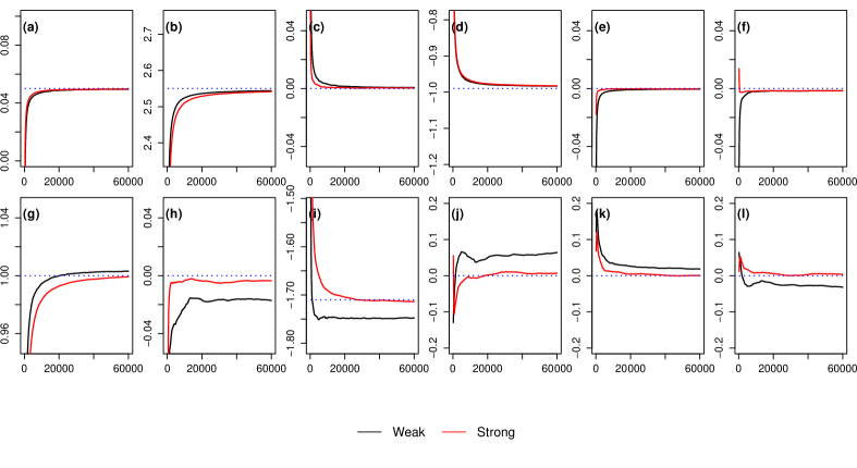
Figure 2: Weak and strong borrowing corresponds to the averages in black and red, respectively. In Fig. 2(a)-(f) and 2(g)-(l) we present the ergodic averages of the control parameters for the maps $C_{1}$ and $Q_{1}$, respectively. True control parameter values are represented by blue horizontal dotted lines.

Table 1: PAREs for the PD-GSBR estimation of the control parameters of the $C_{1}:{\boldsymbol{x}}_{1}^{200}$ and $Q_{1}:{\boldsymbol{x}}_{2}^{50}$ maps. The estimation is based on quintic polynomial modeling, under weak and strong borrowing priors over the selection-probabilities.

Borr.	Map	$\theta_{j0}$	$\theta_{j1}$	$\theta_{j2}$	$\theta_{j3}$	$\theta_{j4}$	$\theta_{j5}$	$\bar{\theta}$
Weak	$C_{1}$	$0.44$	$0.09$	$0.04$	$0.40$	$0.02$	$0.14$	$0.19$
	$Q_{1}$	$0.55$	$1.57$	$2.39$	$6.44$	$1.81$	$3.24$	$2.67$
Strong	$C_{1}$	$0.50$	$0.11$	$0.06$	$0.50$	$0.03$	$0.17$	$0.23$
	$Q_{1}$	$0.23$	$0.25$	$0.48$	$0.57$	$0.01$	$0.42$	$0.37$

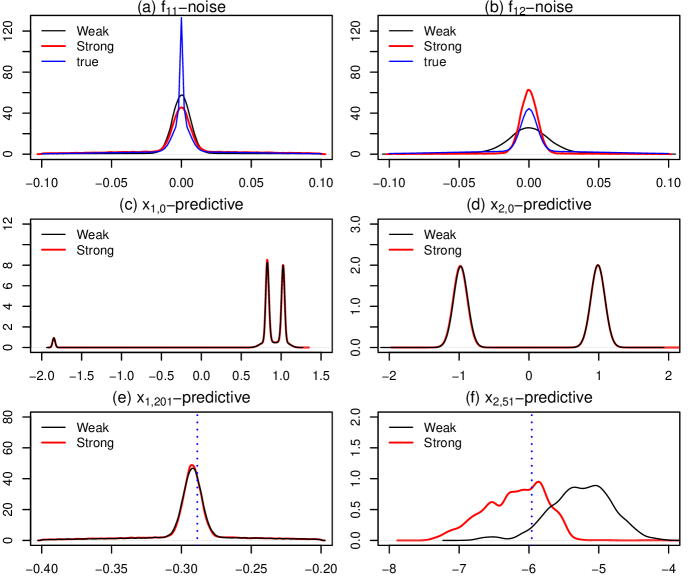
Figure 3: Weak and strong borrowing corresponds to densities in black and red, respectively. Fig. 3(a), 3(c) and 3(e), correspond to map $C_{1}$, and Fig. 3(b), 3(d) and 3(f) to the short time-series map $Q_{1}$. Noise predictive densities are given in Fig. 3(a)-(b). Initial conditions predictive densities are given in Fig. 3(c)-(d). In Fig. 3(e)-(f), we give the predictive densities of the first future observation. True future values, are represented by vertical dotted blue lines.

In Fig. 3(a)-(b), we present kernel density estimations (KDEs) of the marginal noise densities based on noise predictive samples, under weak and strong prior specifications in black and red, respectively. True noise densities are represented by solid blue curves.

In Fig. 3(c)-(d), we display predictive based KDEs of the marginal posteriors of the initial conditions $x_{10}$ and $x_{20}$. The estimations under the two prior configurations are nearly indistinguishable.

In Fig. 3(e)-(f), we present predictive based KDEs of the marginal posteriors of the out-of-sample variables $x_{1,201}$ and $x_{2,51}$. True future values are represented in vertical dotted blue lines. We can see how more accurate is the estimation of the predictive density of the first future observation based on the short time-series, lying outside the invariant set, under the strong borrowing prior (solid red curve) in Fig. 3(f).

4.2 Borrowing between two cubic maps

Here we have generated a pair of cubic time-series via

$$\left[\begin{array}[]{c}{\boldsymbol{x}}_{1}^{200}\\ {\boldsymbol{x}}_{2}^{30}\\ \end{array}\right]\!\!\sim\!\!\left[\begin{array}[]{c}C_{1}\\ C_{2}\\ \end{array}\right]\!\!+\!\!\left[\!\left[\begin{matrix}0&1\\ 1&0\\ \end{matrix}\right]\!\!\otimes\!\!\left[\begin{matrix}0&M_{12}\\ M_{12}&0\\ \end{matrix}\right]\!\right]\!\cdot\!{\boldsymbol{1}}.$$ (13)

The mixture $M_{12}=0.9{\cal N}(0,\sigma^{2})+0.1{\cal N}(0,(200\sigma)^{2})$ with $\sigma^{2}=10^{-6}$, is playing the rôle of the common noise process. In this example as initial conditions we took $x_{10}=x_{20}=1$.

The perturbed cubic trajectories are depicted in Fig. 4(a)-(b). It can be seen, that both time-series experience noise induced jumps.

Figure 4: The noise perturbed time-series of maps $C_{1}$ and $C_{2}$, are given in Fig. 4(a) and 4(b), respectively.

Weak borrowing: Using the weak prior configuration given in (11), the posterior mean of the matrix of the selection-probabilities is approximated by

$$\mathbb{E}({\boldsymbol{p}}|{\boldsymbol{x}})=\left[\begin{matrix}0.879&0.121\\ 0.100&0.900\end{matrix}\right].$$

In this case the large cubic time-series influences the short cubic time-series by only BoI${}_{2}=10\%$.

In Fig. 5(a)-(f), we display in solid black curves the ergodic averages of the estimated control parameters, under the weak prior specification (11). We can see that the ergodic averages based on the short time-series, given in Fig. 5(g)-(l), exhibit slow convergence.

The associated PAREs of the estimated control parameters with respect to the true values, are given in the first two lines of Table II. We can see that the estimations based on the short time-series exhibit large errors, hindering the identification of map $C_{2}$.

Strong borrowing: To force an a-priori strong borrowing from the map $C_{1}$ to the map $C_{2}$, we set

$${\boldsymbol{p}}_{1}\sim{\cal D}ir(1,10)\,\,\,{\rm and}\,\,\,{\boldsymbol{p}}_{2}\sim{\cal D}ir(10,1).$$ (14)

We have the following prior and posterior means

$$\mathbb{E}({\boldsymbol{p}})=\left[\begin{matrix}0.091&0.909\\ 0.909&0.091\end{matrix}\right],\,\,\,\mathbb{E}({\boldsymbol{p}}|{\boldsymbol{x}})=\left[\begin{matrix}0.005&0.995\\ 0.976&0.024\end{matrix}\right].$$

The prior specification (14), increases borrowing considerably from 10% to $97.6\%$. We remark that the posterior mean of the selection-probabilities for the noise process of $C_{2}$ in the second row of $\mathbb{E}({\boldsymbol{p}}|{\boldsymbol{x}})$, is close to the true selection-probabilities.

In Fig. 5(a)-(f), we can see in solid red curves, the ergodic averages of the control parameters under the strong borrowing scenario. We can see now that the ergodic averages based on the short time-series, given in Fig. 5(g)-(l), are converging fast to the true values. In the last two lines of Table II, we can see that the strong borrowing reduces the average PARE of the control parameters of the short cubic time-series, from 1.14% to a mere 0.10%, thus enabling identification of the map $C_{2}$.

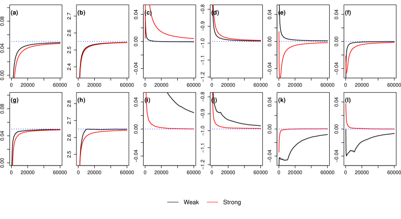
Figure 5: Weak and strong borrowing, corresponds to the averages in black and red, respectively. In Fig. 5(a)-(f) and 5(g)-(l) we present the ergodic averages of the control parameters for the maps $C_{1}$ and $C_{2}$, respectively. True control parameter values, are represented by blue horizontal dotted lines.

Table 2: PAREs for the PD-GSBR estimation of the control parameters of the $C_{1}:{\boldsymbol{x}}_{1}^{200}$ and $C_{2}:{\boldsymbol{x}}_{2}^{30}$ maps. The estimation is based on quintic polynomial modeling, under weak and strong borrowing priors over the selection-probabilities.

Borr.	Map	$\theta_{j0}$	$\theta_{j1}$	$\theta_{j2}$	$\theta_{j3}$	$\theta_{j4}$	$\theta_{j5}$	$\bar{\theta}$
Weak	$C_{1}$	$0.36$	$0.01$	$0.06$	$0.00$	$0.02$	$0.00$	$0.08$
	$C_{2}$	$1.16$	$0.19$	$2.36$	$1.70$	$0.78$	$0.66$	$1.14$
Strong	$C_{1}$	$0.60$	$0.02$	$0.50$	$0.34$	$0.21$	$0.16$	$0.31$
	$C_{2}$	$0.31$	$0.03$	$0.09$	$0.04$	$0.04$	$0.09$	$0.10$

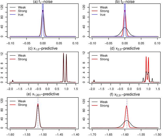
Figure 6: Weak and strong borrowing corresponds to densities in black and red, respectively. Fig. 6(a), 6(c) and 6(e), correspond to map $C_{1}$, and Fig. 6(b), 6(d) and 6(f) to the short time-series map $C_{2}$. Noise predictive densities are given in Fig. 6(a)-(b). Initial conditions predictive densities are given in Fig. 6(c)-(d). In Fig. 6(e)-(f), we give the predictive densities of the first future observation. True future values are represented in vertical dotted blue lines.

In Fig. 6(a)-(b), we present the KDEs of the marginal noise densities based on the noise predictive samples, under weak and strong prior specifications, in black and red solid curves, respectively. True noise densities are represented by solid blue curves. We remark the similarity of the estimated noise densities under the strong prior configuration (14).

In Fig. 6(c)-(d), we display the predictive based KDEs of the marginal posteriors of the initial points $x_{10}$ and $x_{20}$. The estimated marginal posterior density of the variable $x_{20}$, under the weak borrowing prior has five modes. The two spurious modes, disappear after the introduction of strong borrowing (solid curve in red). We remark that the three modes are very close to the three real roots of the polynomial equation $C_{2}(x)-x=0$.

In Fig. 6(e)-(f), we present the predictive based KDEs of the marginal posteriors of the first out-of-sample variables $x_{1,201}$ and $x_{2,31}$. The point estimations of the first out-of-sample values are of the same quality, yet, under strong borrowing the predictive density associated with the short time-series cubic map exhibits a 95% highest posterior density interval (HPDI) shrinkage factor of 0.45. Namely, the weak borrowing HPDI $(-1.622,-1.566)$ of the variable $x_{2,31}$ shrinks to the strong borrowing HPDI $(-1.607,-1.582)$.

4.3 Borrowing between three quadratic maps

For this example we have generated a $3$-multiple perturbed quadratic time-series via

$$\left[\!\begin{array}[]{c}{\boldsymbol{x}}_{1}^{200}\\ {\boldsymbol{x}}_{2}^{20}\\ {\boldsymbol{x}}_{3}^{200}\\ \end{array}\!\right]\!\!\sim\!\!\left[\!\begin{array}[]{c}Q_{3}\\ Q_{2}\\ Q_{1}\\ \end{array}\!\right]\!\!+\!\!\left[\!\left[\begin{matrix}0&1&0\\ 0.90&0&0.10\\ 0&0.33&0.67\\ \end{matrix}\right]\!\!\otimes\!\!\left[\begin{matrix}0&M_{12}&0\\ M_{12}&0&M_{23}\\ 0&M_{23}&M_{33}\\ \end{matrix}\right]\!\right]\!\cdot\!{\boldsymbol{1}}.$$ (15)

The first two time-series have the common part $M_{12}={\cal N}(0,10^{-6})$ and no idiosyncratic parts. The second and third time-series have the common part $M_{23}={\cal N}(0,4\times 10^{-2})$. The third time-series has idiosyncratic part $M_{33}={\cal N}(0,10^{-4})$. In this example as initial conditions we took $x_{10}=x_{20}=1$ and $x_{30}=0.5$.

The three perturbed quadratic trajectories are displayed in Fig. 7(a)-(c).

Figure 7: The noise perturbed time-series for the maps $Q_{3}$, $Q_{2}$ and $Q_{1}$, are given in Fig. 7(a), 7(b) and 7(c), respectively.

Weak borrowing: To force a weak borrowing scenario, a-priori we set for $j=1,2,3$

$${\boldsymbol{p}}_{j}\sim{\cal D}ir({\boldsymbol{\alpha}}_{j}),\,\,\alpha_{ji}=10\,{\cal I}(j=i)+{\cal I}(j\neq i),$$ (16)

with prior mean $\mathbb{E}({\boldsymbol{p}})=10/12\,{\cal I}(j=i)+1/12\,{\cal I}(j\neq i)$. Then the posterior mean after stationarity, is approximated by

$$\mathbb{E}({\boldsymbol{p}}|{\boldsymbol{x}})=\left[\begin{matrix}0.990&0.005&0.005\\ 0.032&0.912&0.056\\ 0.105&0.207&0.688\end{matrix}\right].$$

For $m=3$, we quantify the borrowing of information from the first and third time-series to the second, with the posterior mean BoI${}_{3}:=\mathbb{E}(p_{21}+p_{23}|{\boldsymbol{x}})$. Because, BoI${}_{3}=0.88\%$, the two large time-series have a very small effect on the central short time-series.

In Fig. 8(a)-(r), we display in solid black curves the ergodic averages of the estimated control parameters, under the weak prior specification (16). We can see that the ergodic chains, based on the short time-series, Fig. 8(g)-(l), exhibit serious mixing issues.

The associated PAREs of the estimated control parameters with respect to the true values, are given in the first three lines of Table III. We can see that the estimations based on the short time-series ${\boldsymbol{x}}_{2}^{20}$, exhibit large errors, hindering the identification of the map $Q_{2}$. This situation can be corrected by the introduction of a strong borrowing prior configuration.

Strong borrowing: To force an a-priori strong borrowing from the maps $Q_{3}$ and $Q_{1}$ to the map $Q_{2}$, and at the same time to be noninformative on the selection-probabilities of $Q_{2}$, we set for $j=1,2,3$

$${\boldsymbol{p}}_{j}\sim{\cal D}ir({\boldsymbol{\alpha}}_{j}),\,\,\alpha_{ji}=10\,{\cal I}((j,i)\in J)+{\cal I}((j,i)\notin J),$$ (17)

where $J=\{(j,i):j\neq 2,i=2\}$. We have the following prior and posterior means

$$\mathbb{E}({\boldsymbol{p}})=\left[\begin{matrix}0.083&0.834&0.083\\ 0.333&0.334&0.333\\ 0.083&0.834&0.083\end{matrix}\right],$$

and

$$\mathbb{E}({\boldsymbol{p}}|{\boldsymbol{x}})=\left[\begin{matrix}0.005&0.990&0.005\\ 0.849&0.045&0.106\\ 0.125&0.692&0.183\end{matrix}\right].$$

The prior specification (17) increases borrowing from BoI${}_{3}=0.88\%$ to $95.5\%$. We remark how close is the posterior mean of the selection-probabilities for the noise process of $Q_{2}$, in the second row of $\mathbb{E}({\boldsymbol{p}}|{\boldsymbol{x}})$, to the true selection- probabilities in (15).

In Fig. 8(a)-(r), we can see in solid red curves the ergodic averages of the control parameters, under the strong borrowing scenario. We can see now that the ergodic averages based on the short time-series, given in Fig. 8(g)-(l), are converging fast to the true values. In the last three lines of Table III, we can see that strong borrowing reduces the average PARE of the control parameters of the short time-series, from 12.87% to a mere 0.17% enabling the identification of the map $Q_{2}$.

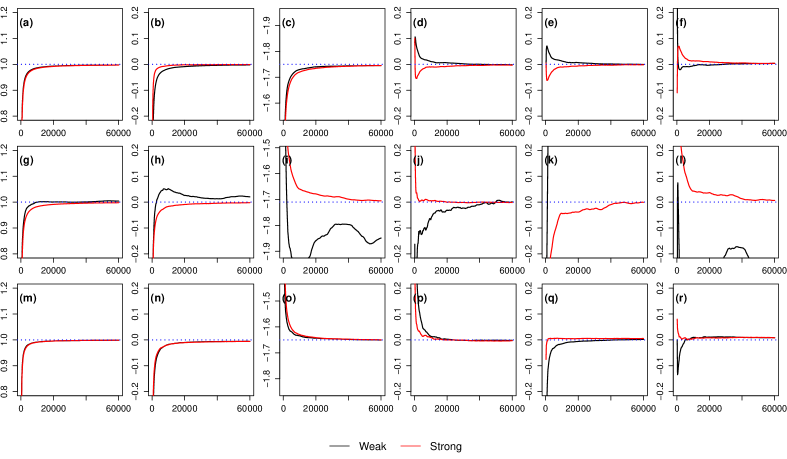
Figure 8: Weak and strong borrowing corresponds to the averages in black and red solid curves, respectively. In Fig. 8(a)-(f), 8(g)-(l) and 8(m)-(r) we present the ergodic averages of the control parameters for the maps $Q_{3}$, $Q_{2}$ and $Q_{1}$, respectively. True control parameter values are represented by horizontal dotted blue lines.

Table 3: PAREs for the PD-GSBR estimation of the control parameters of the $Q_{3}:{\boldsymbol{x}}_{1}^{200}$, $Q_{2}:{\boldsymbol{x}}_{2}^{20}$ and $Q_{1}:{\boldsymbol{x}}_{2}^{200}$ maps. The estimation is based on quintic polynomial modeling, under weak and strong borrowing priors over the selection-probabilities.

Borr.	Map	$\theta_{j0}$	$\theta_{j1}$	$\theta_{j2}$	$\theta_{j3}$	$\theta_{j4}$	$\theta_{j5}$	$\bar{\theta}$
Weak	$Q_{3}$	$0.00$	$0.00$	$0.02$	$0.14$	$0.00$	$0.22$	$0.06$
	$Q_{2}$	$0.62$	$2.38$	$8.51$	$0.33$	$38.17$	$27.19$	$12.87$
	$Q_{1}$	$0.02$	$0.35$	$0.25$	$0.49$	$0.54$	$0.84$	$0.41$
Strong	$Q_{3}$	$0.02$	$0.05$	$0.04$	$0.37$	$0.19$	$0.49$	$0.19$
	$Q_{2}$	$0.05$	$0.01$	$0.11$	$0.27$	$0.17$	$0.39$	$0.17$
	$Q_{1}$	$0.03$	$0.35$	$0.27$	$0.54$	$0.56$	$0.87$	$0.43$

In Fig. 9(a)-(c), we display the KDEs based on the marginal noise predictive samples. In Fig. 9(d)-(f), we display the KDEs based on the marginal initial conditions variable samples. In Fig. 9(g)-(i), we exhibit the KDEs based on the marginal posterior samples of the first out-of-sample variables. Black and red solid curves, refer to weak and strong borrowing priors, respectively. In Fig. 9(b), we have superimposed the noise predictives coming from the weak and strong borrowing scenarios together with the true density of the noise component, given by $0.9M_{12}+0.1M_{23}$, in black, red and blue solid curves, respectively. We note how close to the true noise density, is the density estimated under strong borrowing. In Fig. 9(e), the KDE based on the marginal posterior predictive of the initial condition sample under the strong borrowing prior, has its modes very close to $-1$ and 1. In Fig. 9(h), the estimation of the first out-of-sample value under the strong borrowing prior, exhibits a shrinked 95% HPDI at $(0.484,0.503)$.

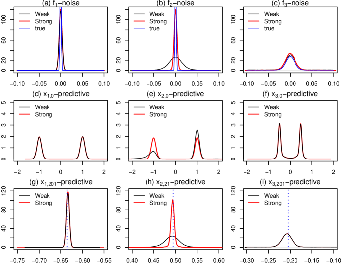
Figure 9: Weak and strong borrowing corresponds to densities in black and red, respectively. Fig. 9(a), 9(d) and 9(g), correspond to map $C_{3}$, Fig. 9(b), 9(e) and 9(h) to the short time-series map $C_{2}$, and Fig. 9(c), 9(f) and 9(i) to map $C_{1}$ Noise predictive densities are given in Fig. 9(a)-(c). Initial conditions predictive densities are given in Fig. 9(d)-(f). In Fig. 9(g)-(i), we display the predictive densities of the first future observation. True future values, are represented by vertical dotted blue lines.

5 Conclusions

We have proposed a new Bayesian nonparametric model, for the joint pairwise dependent reconstruction of dynamical equations, based on observed chaotic time-series data contaminated by dynamical noise. Also, we have introduced a joint parametric Gibbs sampler. In this case the dynamical noise is assumed to be Gaussian, coming from the same noise source for each time-series. Then borrowing of strength, comes from the full conditional of the common precision.

Our numerical experiments, are indicating, that when the densities of the noise processes have common characteristics, underrepresented time series for which an independent Bayesian nonparametric estimation is problematic, can benefit in terms of model estimation accuracy. This can be done by imposing strong borrowing prior specifications between the selection-probabilities of the noise processes of the short time-series, and the time-series with an adequate number of observations for independent Bayesian nonparametric estimation.

Our model can be generalized to include all possible dependencies between the components of the noise processes. For example, consider the set $[m]_{j}$ of the first $m$ natural numbers, except $j$, for $1\leq j\leq m$. We define the set, $C_{mjl}$, of combinations without replacement, over the set of symbols $[m]_{j}$, $l$ at a time, with $0\leq l\leq m-1$, and $C_{mj0}=\emptyset$. Now to each combination $\eta\in C_{mjl}$, we add the symbol $j$, and order the resulting sequence of numbers to $\eta^{*}$, we set $C_{mjl}^{*}=\{\eta^{*}:\eta\in C_{mjl}\}$. The set $C_{mjl}^{*}$ contains the indexes of all possible interactions of the noise process $f_{j}$ of order $l+1$. Then the nonparametric prior over the $j$th noise process can be written as $f_{j}(z)=\int_{v>0}{\cal N}(z|0,v^{-1})\mathbb{Q}_{j}(dv)$, with

$$\mathbb{Q}_{j}=\sum_{l=0}^{m-1}\sum_{\xi\in C_{mjl}^{*}}p_{j,\xi}\,\mathbb{G}_{\xi},\quad\mathbb{G}_{\xi}\stackrel{{\scriptstyle{\rm ind.}}}{{\sim}}{\cal GSB}(\alpha_{\xi},\beta_{\xi},G_{0}).$$

and $\sum_{l=0}^{m-1}\sum_{\xi\in C_{mjl}^{*}}p_{j,\xi}=1$ a.s. Then the $f_{j}$ density, will be the random mixture of the $2^{m-1}$ GSB random mixtures $M_{\xi}$ for $\xi\in C_{mjl}^{*}$. The total number of the independent GSB processes needed to model $\boldsymbol{f}$, will be $2^{m}-1$.

Appendix A Proofs of propositions

Proof of Proposition 1. Augmenting the random densities given in (6) with $N_{ji}$ we have:

$$\Pi(x_{ji},N_{ji}=r\,|\,{\cal R}_{j},x_{j,i-1},\theta_{j})=\sum_{l=1}^{m}\Pi(x_{ji},N_{ji}=r,\delta_{ji}=l\,|\,{\cal R}_{j},x_{j,i-1},\theta_{j})$$

$$=\sum_{l=1}^{m}\Pi(\delta_{ji}=l)\sum_{k=1}^{\infty}\Pi(x_{ji},N_{ji}=r,d_{ji}=k\,|\,{\cal R}_{j},x_{j,i-1},\delta_{ji}=l,\theta_{j})$$

$$=\sum_{l=1}^{m}p_{jl}\sum_{k=1}^{\infty}\Pi(N_{ji}=r\,|\,{\cal R}_{j},\delta_{ji}=l)\Pi(d_{ji}=k\,|\,N_{ji}=r)\Pi(x_{ji}\,|\,x_{j,i-1},d_{ji}=k,\delta_{ji}=l,\theta_{j})$$

$$=\sum_{l=1}^{m}p_{jl}\sum_{k=1}^{\infty}{\cal NB}(N_{ji}=r\,|\,2,\lambda_{jl})\,{\cal DU}(k|1,r)\,{\cal N}(x_{ji}\,|\,g_{j}(\theta_{j},x_{j,i-1}),\tau_{jlk}^{-1})$$

$$=\sum_{l=1}^{m}p_{jl}\sum_{k=1}^{r}\lambda_{jl}^{2}(1-\lambda_{jl})^{r-1}\,{\cal N}(x_{ji}\,|\,g_{j}(\theta_{j},x_{j,i-1}),\tau_{jlk}^{-1}),$$

where ${\cal DU}(k|1,r)=r^{-1}{\cal I}(k\leq r)$ is the discrete uniform distribution, over the set $\{1\ldots,r\}$. Then, it is clear that the $(N_{ji},d_{ji},\delta_{ji})$-augmented density is given by (7). $\square$

Proof of Proposition 2.
1. From equation (7), in vector notation for $\delta_{ji}$, it is that

$$\Pi (x_{ji},N_{ji},d_{ji}|{\cal R}_{j},\delta_{ji},x_{j,i-1},\theta_{j})={\cal I}(d_{ji}\leq N_{ji})$$

$$\times\prod_{l=1}^{m}\left\{\lambda_{jl}^{2}\,(1-\lambda_{jl})^{N_{ji}-1}{\cal N}(x_{ji}\,|\,g_{j}(\theta_{j},x_{j,i-1}),\tau_{jld_{ji}}^{-1})\right\}^{\delta_{ji}^{l}}.$$

The desired result comes from the substitution of the last equation in the conditional likelihood expression

$$\Pi ({\boldsymbol{x}}^{\prime},{\boldsymbol{x}},\,{\boldsymbol{N}},{\boldsymbol{d}}\,|\,{\cal R},{\boldsymbol{\delta}},{\boldsymbol{\theta}},{\boldsymbol{x}}_{0})$$

$$=\prod_{j=1}^{m}\prod_{i=1}^{n_{j}+T_{j}}\Pi(x_{ji},N_{ji},d_{ji}\,|\,{\cal R}_{j},\delta_{ji},x_{j,i-1},\theta_{j}).$$

2. Fixing the random selection probabilities to $p_{jl}=1/(m-1)\,{\cal I}(l<j)$ and the random mixing measures to $\mathbb{G}_{jl}=\delta_{\tau}$ a.s., it is that

$$\Pi({\boldsymbol{x}}^{\prime},{\boldsymbol{x}}\,|\,{\boldsymbol{\theta}},{\boldsymbol{x}}_{0})=\prod_{j=1}^{m}\prod_{i=1}^{n_{j}+T_{j}}\Pi(x_{ji}\,|\,x_{j,i-1},\theta_{j}),$$

with $\Pi(x_{ji}\,|\,x_{j,i-1},\theta_{j})={\cal N}(x_{ji}\,|\,0,\tau^{-1})$, which gives the desired result. $\square$

Appendix B Full conditional distributions for the PD-GSBR Gibbs sampler

In this appendix we describe the PD-GSBR Gibbs sampler. At each iteration of the Gibbs sampler we will sample the variables:

$$\tau_{jlk},1\leq j\leq l\leq m,\,1\leq k\leq N^{*},$$

$$N_{ji},d_{ji},\delta_{ji},1\leq j\leq m,\,1\leq i\leq n_{j}+T_{j},$$

$$p_{jl},1\leq j\leq m,1\leq l\leq m,$$

$$\vartheta_{j},x_{j0},1\leq j\leq m$$

with $N^{*}:=\max_{j,i}N_{ji}$ a.s. finite. Having in mind that for ${\cal R}=\{{\boldsymbol{p}},{\boldsymbol{\lambda}},{\boldsymbol{\tau}}^{\infty}\}$ the $({\boldsymbol{N}},{\boldsymbol{d}},\,{\boldsymbol{\delta}})$-augmented posterior is proportional to

$$\Pi({\boldsymbol{p}})\Pi({\boldsymbol{\lambda}}) \Pi({\boldsymbol{\tau}}^{\infty})\Pi({\boldsymbol{\theta}})\Pi({\boldsymbol{x}}_{0})\Pi({\boldsymbol{\delta}}|{\boldsymbol{p}})$$

$$\times\Pi({\boldsymbol{x}}^{\prime},{\boldsymbol{x}},\,{\boldsymbol{N}},{\boldsymbol{d}}\,|\,{\boldsymbol{p}},{\boldsymbol{\lambda}},{\boldsymbol{\tau}}^{\infty},{\boldsymbol{\delta}},{\boldsymbol{\theta}},{\boldsymbol{x}}_{0}),$$

and taking into account (8) and (9) we have the following:

1. Letting ${\cal H}_{jilk}:={\cal N}(x_{ji}|g_{j}(\theta_{j},x_{j,i-1}),\tau_{jlk}^{-1})$, and ${\cal I}_{jilk}:={\cal I}(\delta_{ji}=\mathbf{e}_{l},d_{ji}=k)$, the full conditionals for the precisions $\tau_{jlk}$, for $k=1,\ldots,N^{*}$ and $1\leq j\leq l\leq m$, are given by

$$\Pi(\tau_{jlk}|\cdots)\propto\,\Pi(\tau_{jlk})\prod_{i=1}^{n_{j}}{\cal H}_{jilk}^{{\cal I}_{jilk}}\prod_{i=1}^{n_{l}}{\cal H}_{jilk}^{{\cal I}(j<l){\cal I}_{lijk}},$$ (18)

where $\Pi(\tau_{jlk}|\cdots)$ denotes the dependence of the variable $\tau_{jlk}$ to the rest of the variables. Standard Bayesian modeling suggests, the use of gamma conjugate prior distributions over the $\tau_{jlk}$’s, so, we set $\tau_{jlk}\sim g_{0}={\cal G}(a,b)$, where $g_{0}$ stands for the density of the mean measure $G_{0}$ which is a gamma density with shape $a$, rate $b$. Then, letting $h_{\theta_{j}}(x_{ji},x_{j,i-1}):=(x_{ji}-g_{j}(\theta_{j},x_{j,i-1}))^{2}$, it is not difficult to verify that the full conditional of $\tau_{jlk}$ is gamma with shape

$$a+{1\over 2}\sum_{i=1}^{n_{j}}{\cal I}_{jilk}+{1\over 2}{\cal I}(j<l)\sum_{i=1}^{n_{l}}{\cal I}_{lijk},$$

and rate

$$b +{1\over 2}\sum_{i=1}^{n_{j}}{\cal I}_{jilk}\,h_{\theta_{j}}(x_{ji},x_{j,i-1})$$

$$+{1\over 2}{\cal I}(j<l)\sum_{i=1}^{n_{l}}\,{\cal I}_{lijk}\,h_{\theta_{l}}(x_{li},x_{l,i-1}).$$

2. Next, we will sample the mixture allocation variables $d_{ji}$ and the mixture component indicator variables $\delta_{ji}$ as a block. For $j=1,\ldots,m$ and $i=1,\ldots,n_{j}+T_{j},$ it is that

$${\rm P}\{d_{ji}=k,\delta_{ji}=\mathbf{e}_{l}|\cdots\}\propto p_{jl}\,{\cal H}_{jilk}\,{\cal I}(l\leq m)\,{\cal I}(k\leq N_{ji}).$$

3. The geometric-slice variables $N_{ji}$ have full conditional distributions that are given by

$${\rm P}\{N_{ji}=r|\delta_{ji}=\mathbf{e}_{l},d_{ji}=l,\cdots\}\propto(1-\lambda_{jl})^{r}\,{\cal I}(l\leq r),$$

which are truncated geometric distributions over the set $\{l,l+1,\ldots\}$.

4. The full conditional for the selection-probabilities ${\boldsymbol{p}}_{j}$, $j=1,\ldots,m$, under the conjugate Dirichlet prior

$$\Pi({\boldsymbol{p}}_{j})={\cal D}ir({\boldsymbol{p}}_{j}|{\boldsymbol{\alpha}}_{j})={\Gamma(\alpha_{j1}+\cdots+\alpha_{jm})\over\Gamma(\alpha_{j1})\cdots\Gamma(\alpha_{jm})}\prod_{l=1}^{m}p_{jl}^{\alpha_{jl}-1},$$

with fixed hyperparameter ${\boldsymbol{\alpha}}_{j}=(\alpha_{j1},\dots,\alpha_{jm})$, supported over the probability simplex $\{{\boldsymbol{p}}_{j}\in(0,1)^{m}:\sum_{l=1}^{m}p_{jl}=1\}$, is the Dirichlet distribution

$$\Pi({\boldsymbol{p}}_{j}|\cdots)\,\propto\,\prod_{l=1}^{m}p_{jl}^{\alpha_{jl}+\sum_{i=1}^{n_{l}}{\cal I}(\delta_{ji}\,=\,\mathbf{e}_{l})-1}.$$

5. The full conditionals for the geometric-probabilities $\lambda_{jl}$’s, under beta conjugate priors $\lambda_{jl}\sim{\cal B}e(a_{jl},b_{jl})$, are beta distributions. Defining $S_{jl}:=\sum_{i=1}^{n_{j}}{\cal I}(\delta_{ji}={\bf e}_{l})$ and $S_{jl}^{\prime}:=\sum_{i=1}^{n_{j}}{\cal I}(\delta_{ji}={\bf e}_{l})(N_{ji}-1)$, it is that

$$f(\lambda_{jl}|\cdots)={\cal B}e(\lambda_{jl}|a_{jl} +2(S_{jl}+S_{lj}{\cal I}(l<j)),$$

$$b_{jl}+(S_{jl}^{\prime}+S_{lj}^{\prime}{\cal I}(l<j))).$$

6. For the vectors of control parameters $\theta_{j}$ $1\leq j\leq m$ the full conditional becomes

$$\Pi(\theta_{j}|\cdots)\propto\Pi(\theta_{j})\exp\{-\frac{1}{2}\sum_{i=1}^{n_{j}+T_{j}}\tau_{jld_{ji}}h_{\theta_{j}}(x_{ji},x_{j,i-1})\}.$$ (19)

7. The full conditional for $x_{j0}$ will be

$$\Pi(x_{j0}\,|\,\cdots)\propto\Pi(x_{j0})\exp\left\{-\frac{\tau_{jld_{1}}}{2}h_{\theta{j}}(x_{j1},x_{j0})\right\}.$$ (20)

8. The full conditionals for the sampling of the out-of-sample observations for $k=1,\ldots,T_{j}-1$ are given by

$$\Pi(x_{j,n_{j}+k}|\cdots) \propto\exp\left\{-\frac{1}{2}\left[\tau_{d_{j,n_{j}+k}}h_{\theta_{j}}(x_{n_{j}+k},x_{n_{j}+k-1})\right.\right.$$

$$+\left.\left.\tau_{d_{j,n_{j}+k+1}}h_{\theta_{j}}(x_{n_{j}+k+1},x_{n_{j}+k})\right]\right\}.$$ (21)

Also, for $k=T_{j}$, the full conditional is normal, with mean $g_{j}(\theta_{j},x_{j,n_{j}+T_{j}-1})$, and variance $\tau_{j\delta_{j,n_{j}+T_{j}}d_{j,n_{j}+T_{j}}}^{-1}$.

9. Having updated the selection probabilities to ${\boldsymbol{p}}^{*}$, and the geometric probabilities to ${\boldsymbol{\lambda}}^{*}$, we construct the geometric weights $(\pi_{jlk}^{*})_{1\leq j\leq N^{*}}$ via equation (3). Defining

$$\pi_{jl,N^{*}+1}^{*}=1-\sum_{k=1}^{N^{*}}\pi_{jlk}^{*}\quad{\rm and}\quad\tau_{jl,N^{*}+1}^{*}\sim g_{0},$$

we are now ready to sample each $Z_{j,n_{j}+1}$ from its noise predictive

$$Z_{j,n_{j}+1} \sim f_{j}(\,\cdot\,|{\boldsymbol{x}})=\sum_{l=1}^{m}p_{jl}^{*}M_{jl}^{*}(\,\cdot\,|{\boldsymbol{x}}),$$

$${\rm with}\quad M_{jl}^{*}(z|{\boldsymbol{x}})=\sum_{k=1}^{N^{*}+1}\pi_{jlk}^{*}{\cal N}(z|0,(\tau_{jlk}^{*})^{-1}).$$

At each iteration of the Gibbs sampler, and for each $j$, we sample independently $\rho_{j},\rho_{j}^{\prime}\stackrel{{\scriptstyle{\rm i.i.d.}}}{{\sim}}{\cal U}(0,1)$. So, $Z_{j,n_{j}+1}$, will be sampled from the a.s. finite mixture $M_{jl}^{*}(\,\cdot\,|{\boldsymbol{x}})$, with $1\leq l\leq m$, satisfying

$$\sum_{r=0}^{l-1}p_{jr}^{*}<\rho_{j}\leq\sum_{r=0}^{l}p_{jr}^{*},\,\,\,p_{j0}^{*}=0,$$

and from the $k$-th normal component ${\cal N}(\,\cdot\,|0,(\tau_{jlk}^{*})^{-1})$ of the $M_{jl}^{*}(\,\cdot\,|{\boldsymbol{x}})$ mixture, with $1\leq k\leq N^{*}+1$, satisfying

$$\sum_{r=0}^{k-1}\pi_{jlr}^{*}<\rho_{j}^{\prime}\leq\sum_{r=0}^{k}\pi_{jlr}^{*},\,\,\,\pi_{jl0}^{*}=0.$$

Details on sampling efficiently via embedded Gibbs samplers, thus circumventing Metropolis-within-Gibbs implementations for the nonstandard densities arising in equation (19) through (21), are provided in the supplementary file of Merkatas, Kaloudis, and Hatjispyros (2017).

References

• Ott (2002) E. Ott, Chaos in dynamical systems (Cambridge university press, 2002).
• Berliner (1992) L. M. Berliner, “Statistics, probability and chaos,” Statistical Science , 69–90 (1992).
• Chatterjee and Yilmaz (1992) S. Chatterjee and M. R. Yilmaz, “Chaos, fractals and statistics,” Statistical Science , 49–68 (1992).
• Mees (2012) A. I. Mees, Nonlinear dynamics and statistics (Springer Science & Business Media, 2012).
• Ruelle and Takens (1971) D. Ruelle and F. Takens, “On the nature of turbulence,” Communications in mathematical physics 20, 167–192 (1971).
• Abarbanel (2012) H. Abarbanel, Analysis of observed chaotic data (Springer Science & Business Media, 2012).
• Kantz and Schreiber (2004) H. Kantz and T. Schreiber, Nonlinear time-series analysis, Vol. 7 (Cambridge university press, 2004).
• Jaeger and Kantz (1997) L. Jaeger and H. Kantz, “Homoclinic tangencies and non-normal jacobians—effects of noise in nonhyperbolic chaotic systems,” Physica D: Nonlinear Phenomena 105, 79–96 (1997).
• Arnold (1998) L. Arnold, “emph “bibinfo title Random dynamical systems, Springer Monographs in Mathematics (Springer-Verlag, Berlin, 1998) pp. xvi+586.
• Smith and Mees (2000) L. Smith and A. Mees, “Nonlinear dynamics and statistics,” Disentangling Uncertainty and Error: On the Predictability of Nonlinear Systems, Birkhäuser, Boston  (2000).
• He and Habib (2013) T. He and S. Habib, “Chaos and noise,”  Chaos: An Interdisciplinary Journal of Nonlinear Science  23, 033123 (2013).
• Muldoon et al. (1998) M. R. Muldoon, D. S. Broomhead, J. P. Huke,  and R. Hegger, “Delay embedding in the presence of dynamical noise,” Dynamics and Stability of Systems 13, 175–186 (1998).
• Siegert, Friedrich, and Peinke (1998) S. Siegert, R. Friedrich,  and J. Peinke, “Analysis of data sets of stochastic systems,” arXiv preprint cond-mat/9803250  (1998).
• Siefert and Peinke (2004) M. Siefert and J. Peinke, “Reconstruction of the deterministic dynamics of stochastic systems,” International Journal of Bifurcation and Chaos 14, 2005–2010 (2004).
• Heald and Stark (2000) J. Heald and J. Stark, “Estimation of noise levels for models of chaotic dynamical systems,” Physical review letters 84, 2366 (2000).
• Strumik and Macek (2008) M. Strumik and W. M. Macek, “Influence of dynamical noise on time-series generated by nonlinear maps,” Physica D: Nonlinear Phenomena 237, 613–618 (2008).
• Siefert et al. (2004) M. Siefert, M. Kern, R. Friedrich,  and J. Peinke, “How to differentiate quantitatively between nonlinear dynamics, dynamical noise and measurement noise,” in EXPERIMENTAL CHAOS: 8th Experimental Chaos Conference, Vol. 742 (AIP Publishing, 2004) pp. 337–344.
• Robert (2007) C. Robert, The Bayesian choice: from decision-theoretic foundations to computational implementation (Springer Science & Business Media, 2007).
• Davies (1998) M. Davies, “Nonlinear noise reduction through monte carlo sampling,” Chaos: An Interdisciplinary Journal of Nonlinear Science 8, 775–781 (1998).
• Meyer and Christensen (2000) R. Meyer and N. Christensen, “Bayesian reconstruction of chaotic dynamical systems,” Physical Review E 62, 3535 (2000).
• Meyer and Christensen (2001) R. Meyer and N. Christensen, “Fast bayesian reconstruction of chaotic dynamical systems via extended kalman filtering,” Physical Review E 65, 016206 (2001).
• McSharry and Smith (1999) P. E. McSharry and L. A. Smith, “Better nonlinear models from noisy data: Attractors with maximum likelihood,” Physical Review Letters 83, 4285 (1999).
• Smelyanskiy et al. (2005) V. Smelyanskiy, D. G. Luchinsky, D. Timucin,  and A. Bandrivskyy, “Reconstruction of stochastic nonlinear dynamical models from trajectory measurements,” Physical Review E 72, 026202 (2005).
• Luchinsky et al. (2008) D. G. Luchinsky, V. N. Smelyanskiy, A. Duggento,  and P. V. McClintock, “Inferential framework for nonstationary dynamics. i. theory,” Physical Review E 77, 061105 (2008).
• Matsumoto et al. (2001) T. Matsumoto, Y. Nakajima, M. Saito, J. Sugi,  and H. Hamagishi, “Reconstructions and predictions of nonlinear dynamical systems: A hierarchical bayesian approach,” IEEE transactions on signal processing 49, 2138–2155 (2001).
• Nakada et al. (2005) Y. Nakada, T. Matsumoto, T. Kurihara,  and K. Yosui, “Bayesian reconstructions and predictions of nonlinear dynamical systems via the hybrid monte carlo scheme,” Signal processing 85, 129–145 (2005).
• Molkov et al. (2012) Y. Molkov, E. Loskutov, D. Mukhin,  and A. Feigin, “Random dynamical models from time-series,” Physical Review E 85, 036216 (2012).
• Shinde and Gupta (1974) M. Shinde and S. Gupta, “Signal detection in the presence of atmospheric noise in tropics,” IEEE Transactions on Communications 22, 1055–1063 (1974).
• Middleton (1977) D. Middleton, “Statistical-physical models of electromagnetic interference,” IEEE Transactions on Electromagnetic Compatibility , 106–127 (1977).
• Kanazawa et al. (2015a) K. Kanazawa, T. G. Sano, T. Sagawa,  and H. Hayakawa, “Minimal model of stochastic athermal systems: Origin of non-gaussian noise,” Physical review letters 114, 090601 (2015a).
• Kaloudis and Hatjispyros (2018) K. Kaloudis and S. J. Hatjispyros, “A Bayesian nonparametric approach to dynamical noise reduction,” Chaos: An Interdisciplinary Journal of Nonlinear Science  28, 063110 (2018).
• Kanazawa et al. (2015b) K. Kanazawa, T. G. Sano, T. Sagawa,  and H. Hayakawa, “Asymptotic derivation of langevin-like equation with non-gaussian noise and its analytical solution,” Journal of Statistical Physics 160, 1294–1335 (2015b).
• Rodriguez and Ter Horst (2008) A. Rodriguez and E. Ter Horst, “Bayesian dynamic density estimation,” Bayesian Analysis 3, 339–365 (2008).
• Taddy and Kottas (2009) M. A. Taddy and A. Kottas, “Markov switching Dirichlet process mixture regression,” Bayesian Analysis 4, 793–816 (2009).
• Jensen and Maheu (2010) M. J. Jensen and J. M. Maheu, “Bayesian semiparametric stochastic volatility modeling,” Journal of Econometrics 157, 306–316 (2010).
• Griffin (2010) J. E. Griffin, “Inference in infinite superpositions of non–Gaussian Ornstein–Uhlenbeck processes using Bayesian nonparametic methods,” Journal of Financial Econometrics 9, 519–549 (2010).
• Mena, Ruggiero, and Walker (2011) R. H. Mena, M. Ruggiero,  and S. G. Walker, “Geometric stick–breaking processes for continuous–time Bayesian nonparametric modeling,” Journal of Statistical Planning and Inference 141, 3217–3230 (2011).
• Fox et al. (2009) E. Fox, M. I. Jordan, E. B. Sudderth,  and A. S. Willsky, “Sharing features among dynamical systems with Beta processes,” Advances in Neural Information Processing Systems , 549–557 (2009).
• Fox et al. (2008) E. B. Fox, E. B. Sudderth, M. I. Jordan,  and A. S. Willsky, “An HDP–HMM for systems with state persistence,” in Proceedings of the 25th international conference on Machine learning (ACM, 2008) pp. 312–319.
• Nieto-Barajas and Quintana (2016) L. E. Nieto-Barajas and F. A. Quintana, “A Bayesian non-parametric dynamic AR model for multiple time-series analysis,” Journal of Time Series Analysis 37, 675–689 (2016).
• Merkatas, Kaloudis, and Hatjispyros (2017) C. Merkatas, K. Kaloudis,  and S. J. Hatjispyros, “A Bayesian nonparametric approach to reconstruction and prediction of random dynamical systems,” Chaos: An Interdisciplinary Journal of Nonlinear Science 27, 063116 (2017).
• Ferguson (1973) T. S. Ferguson, “A bayesian analysis of some nonparametric problems,” The annals of statistics , 209–230 (1973).
• Sethuraman (1994) J. Sethuraman, “A constructive definition of dirichlet priors,” Statistica sinica , 639–650 (1994).
• Fuentes-García, Mena, and Walker (2010) R. Fuentes-García, R. H. Mena,  and S. G. Walker, “A new Bayesian nonparametric mixture model,” “bibfield journal “bibinfo journal Comm. Statist. Simulation Comput.“ “textbf “bibinfo volume 39,“ “bibinfo pages 669–682“ (“bibinfo year 2010).
• Hatjispyros et al. (2017) S. J. Hatjispyros, C. Merkatas, T. Nicoleris,  and S. G. Walker, “Dependent mixtures of geometric weights priors,” Computational Statistics & Data Analysis 119, 1–18 (2017).