Regularizing a linearized EIT reconstruction method using a sensitivity based factorization method
Abstract
For electrical impedance tomography (EIT), most practical reconstruction methods are based on linearizing the underlying non-linear inverse problem. Recently, it has been shown that the linearized problem still contains the exact shape information. However, the stable reconstruction of shape information from measurements of finite accuracy on a limited number of electrodes remains a challenge.
In this work we propose to regularize the standard linearized reconstruction method (LM) for EIT using a non-iterative shape reconstruction method (the factorization method). Our main tool is a discrete sensitivity-based variant of the factorization method (herein called S-FM) which allows us to formulate and combine both methods in terms of the sensitivity matrix. We give a heuristic motivation for this new method and show numerical examples that indicate its good performance in the localization of anomalies and the alleviation of ringing artifacts.
keywords:
electrical impedance tomography; regularization; linearized reconstruction method; factorization methodThis is an Author’s Accepted Manuscript of an article published in Inverse Probl. Sci. Eng. 22(7), 1029–1044, 2014, published online: 01 Nov 2013, ©Taylor & Francis, available online at: http://www.tandfonline.com/doi/abs/10.1080/17415977.2013.850682
35R30; 65F22
1 Introduction
In electrical impedance tomography (EIT), we try to reconstruct the electrical conductivity distribution of an imaging subject from boundary measurements that are collected by placing surface electrodes around the subject, injecting different linearly independent currents using chosen pairs of electrodes, and measuring the required voltages [34, 10, 22]. EIT seems to be a unique technique capable of low-cost measuring continuous real-time tomographic impedance of human body non-invasively. EIT has been used for regional lung function monitoring [3, 36]. Although numerous EIT reconstruction algorithms have been developed last three decades, it has not yet reached a satisfactory level of clinical competency [7, 6, 37, 35, 14, 30, 11, 31, 32, 5, 1, 2, 33, 4].
In EIT, the boundary data-set describing the boundary current-potential relation along the attached electrodes is determined mainly by the boundary geometry, electrode positions and the conductivity distribution. The nonlinear and ill-posed relation between the data-set and the conductivity distribution are entangled with the modeling errors caused by inaccurate boundary geometry, uncertainty in electrode positions, measurement noises, and unknown contact impedance [22]. The ill-posedness and the forward modeling errors can be alleviated by using the difference between a reference data-set and a received data-set to produce a difference image of the conductivity distribution. The most commonly used algorithms in practical EIT systems are linearized reconstruction methods (LM) [24, 10, 22, 2]. They are based on the linearized approximation of the relation between the conductivity difference and the difference data-set
| (1) |
where is the so-called sensitivity matrix (see section 2).
The linearized relation (1) is ill-conditioned. Small error in data produces large error in the reconstructed image. A natural and frequently used regularization strategy is to only reconstruct those features of the image that are least affected by noise which leads to the truncated singular value decomposition (tSVD), see section 2.2. However, this approach is known to lead to strong ringing artifacts around boundaries in the reconstructed images.
Recently, two of authors showed rigorously that the linearized EIT equation contains full information about the shape and position of conductivity anomalies [19]. Hence, linearization should not be the cause for shape and position artifacts. However, this theoretical result requires a continuous sampling on the boundary. In a realistic EIT setting, we have to deal with a limited number of electrodes and with measurement errors. Standard regularization methods as tSVD are not adapted to shape recovery and do not stably recover shape and position information.
The aim of the present work is to enhance the conventional LM by regularizing it with the factorization method that was specifically designed for shape recovery, cf. [26, 9, 8, 15] for the origins of this method, and [28, 17, 21] for recent overviews. Our main tool is a sensitivity matrix based variant of the factorization method (S-FM), that uses the columns of the sensitivity matrix to form a pixel-wise index indicating the possibility of the presence or absence of an anomaly in this pixel. This allows us to formulate and combine the LM and the S-FM in the same framework. We perform various numerical simulations to show that our new combination effectively alleviates ringing artifacts.
2 Method
Let be a two- or three-dimensional domain with -boundary . Assume that is a reference conductivity and is a conductivity distribution with a perturbation on the anomaly , where and denotes the position in .
We begin with the standard linearized method (LM) in -channel EIT system. In order to inject currents into the imaging subject , we attach point electrodes , , on the boundary and inject a current of mA between each pair of adjacent electrodes . For simplicity, we assume and ignore the effects of the unknown contact impedances between electrodes with the boundary. The electrical potential due to the -th current is denoted by and satisfies the following Neumann boundary value problem:
| (2) | |||||
| (3) |
where is the outward unit normal vector on . For the justification and well-posedness of the point electrode model we refer to [16].
We measure a boundary voltage between an adjacent pair of electrodes, and for . The -th boundary voltage difference subject to the -th injection current is denoted as
| (4) |
see our remark on the end of this subsection about evaluating the potential on current-driven electrodes.
Collecting number of boundary voltage data, the measured data-set can be expressed as
| (5) |
Assume that we also have a data-set for the reference conductivity . Let be the solution of (2), (3) with replaced by .
The inverse problem is to reconstruct from the difference . The difference data-set is a response of the anomaly such that
| (6) |
In LM, we use the following approximation
| (7) |
Note that according to the theoretical result in [19], this linearization does not lead to position and shape errors if a continuous sampling on the boundary is available. A EIT system with a limited number of electrodes will always produce shape errors; but the shape errors depend mainly on the configuration of electrodes and the linearization is minor cause of the shape and position errors.
Discretizing the domain into elements as and assuming that and are constants on each element , we obtain from (6) and (7)
| (8) |
where is the value of on the pixel . (See the remark at the end of this section concerning the pixels adjacent to a point electrode.)
(8) can be written as the following linear system
| (9) |
where
Here, is the -th block of the linearized sensitivity matrix:
| (10) |
It is well-known that the sensitivity matrix is ill-conditioned for realistic numbers of pixels and electrodes, so that solving (9) requires regularization.
For the sake of mathematical rigorosity we have to note that, in the point electrode model, the electric potential possesses singularities on current driven electrodes. Hence, the evaluations in (4) and (5) may not be well-defined. Moreover, is not neccessarily square integrable on pixes adjacent to a point electrodes, so that entries of belonging to such boundary pixels might also not be well-defined.
A rigorous mathematical way to overcome the first problem is to note that we only work with the difference data (6). Since , point evaluations of difference data are well-defined, even on current-driven electrodes, see [16]. The second problem can be overcome by replacing the partition by a partition for a slightly smaller open set with that is known to contain the inclusions.
In the scope of this article, we consider both problems to be mathematical subtleties, as we work with numerical approximations to the point electrode model anyway. Hence, for the sake of readability, we stick to the somewhat sloppy formulations above
2.1 Sensitivity matrix based Factorization Method (S-FM)
Though the linearized equation still contains the correct shape information, standard regularization methods for the linear reconstruction method (LM) are not designed for shape reconstruction and tend to produce ringing artifacts around conductivity anomalies. To improve this, we will combine it with the factorization method (FM) which is a non-iterative anomaly detection method that provides a criterion for determining the presence or absence of an anomaly at each location in the imaging subject. Hence, we expect the FM to improve the anomaly detection performance of the standard LM.
Standard formulations of the FM utilize special dipole functions to characterize whether a given point belongs to an anomaly or not. In order to use the FM for regularizing the LM, we develop a sensitivity matrix based factorization method (S-FM). The main idea is that the dipole functions can be replaced by the column vectors of the sensitivity matrix . We will now explain this idea in some detail:
Given a pixel with and the -th injection current, let solve
| (11) |
where is the characteristic function having on and otherwise. can be regarded as a pixel-based analogue to a dipole function which solves .
The boundary voltages of the pixel-based dipole function agree with the column vectors of the sensitivity matrix .
Lemma 2.1.
Denote where
| (12) |
Then and hence
| (13) |
Proof. From the Neumann boundary condition of in (2),(3), we have
| (14) |
for . On the other hand, it follows from the definition of in (11) that
| (15) |
Now, we will derive the pixel-based anomaly detection criterion of S-FM. First, we interpret the values in the data set as a matrix, i.e., we replace the -dimensional vector by the -matrix
| (16) |
To simplify the presentation let us assume in the following that the conductivity difference satisfies the linear approximation , and that is invertible, cf. [20] for a justification of the FM without these assumptions. Moreover, we assume that the conductivity contrast is equal to one inside the inclusion, i.e. , where is compactly supported in .
The following theorem is the basis for the S-FM:
Theorem 2.2.
-
(a)
For all pixel and -th injection current
(17) where .
-
(b)
If the pixel lies inside the inclusion then for all injection currents
(18)
Proof. By lemma 2.1 and superposition we have for all
| (19) |
On the other hand, we can define
| (20) |
and use that
| (21) |
to obtain
| (22) | |||||
Now we are ready to prove the two assertions (a) and (b).
- (a)
- (b)
The estimates in theorem 2.2(a) and (b) provide the following observations that can be viewed as a sensitivity matrix based version of the previous work in [18, 20]:
-
•
If the pixel lies outside the inclusion , then we can expect that there exists an excitation pattern so that the resulting current will be large in the pixel but small inside the inclusion . See [13] for the rigorous mathematical basis of this argument.
Hence, we can expect that for some the expression
will be very large.
-
•
If the pixel lies inside the inclusion , then
will be not so large.
The above observations enable us to predict the presence and absence of anomaly at each location by evaluating
| (23) |
2.2 Hybrid method combining S-FM with LM
Now, we are ready to explain a hybrid method in which S-FM and LM cooperate with each other.
2.2.1 Drawbacks of the standard linearized method
For the image reconstruction using LM, assume that we use tSVD of the form where is a diagonal matrix with the largest singular values , and is a matrix with the first -th columns of the left singular matrix and the right singular matrix , respectively. Here, can be determined by the noise level in the measurements. The smallest singular value must be sufficiently large in such a way that the following reconstruction method is reasonably robust against noise in the data-set :
| (24) |
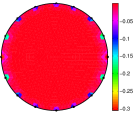
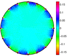
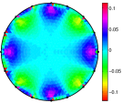
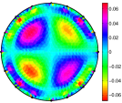
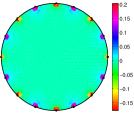
where is the tSVD pseudoinverse of . To explain the underlying idea intuitively, we focus on the standard 16-channel EIT system. In this EIT system, we usually choose which is the number corresponding to . Figure 1 shows a part of images of . Note that the best achievable image by LM would be the projected image of the true into the vector space spanned by as shown in Figure 1. Clearly, the basis is insufficient to achieve localization of conductivity anomalies and causes Gibbs ringing artifacts.
2.2.2 A naive combination of LM and S-FM
To deal with the drawbacks in LM, it seems natural to use the additional information obtained from S-FM as a regularization term, i.e., to
| (25) |
where is a regularization parameter and a positive diagonal matrix having -th entry
| (26) |
Recalling the property of from subsection 2.1, a large value of corresponds to a higher chance of getting . The least squares formulation of (25) takes the form
where is a zero vector. Note that this method tries to make zeros in which a subregion having large value of has a higher likelihood of .
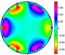
We demonstrate in several numerical examples in the next section that this naive combination of LM and S-FM methods performs better than the standard linearized method, but still produces some ringing artifacts. We believe that this is due to the singular value structure of the matrix . Let the tSVD pseudoinverse of be where and , respectively, is the truncated right and left singular matrix of . There exists a significant difference between the right singular vectors and . Roughly speaking, the right singular vectors of corresponding to high singular values can be viewed as a basis to reconstruct images in the region of those pixels having high values of . Hence, according to S-FM, the right singular vectors associated with high singular values are used to reconstruct images in the region of . On the other hand, the right singular vectors associated with low singular values are used to reconstruct images of anomaly region ( ), that is, the expression of provides image of anomaly region ( ) by a linear combination of right singular vectors associated with low singular values. Thus, may still contain undesirable artifacts as shown in Figure 2.
2.2.3 The proposed combination of LM and S-FM
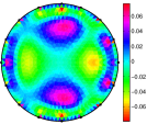
The very intuitve above approach of using the information from the S-FM as a regularization term did not produce satisfactory numerical results. Summing up the above arguments, we believe that this is due to the fact that the right singular vectors (corresponding to the higher singular values) of the resulting linear system tend to have their support outside the anomaly. Based on this idea we try to design a linear system where these vectors tend to have their support inside the anomaly. We suggest to use the following new matrix
| (27) |
where is a positive constant. Based on the above heuristic arguments, we can expect that using the auxiliary matrix should change the singular values in such a way that the right singular vectors of associated with high singular values tend to be useful for reconstructing images in the region of anomaly (i.e. the region with ). Thus, using instead of the sensitivity matrix adds some location information of conductivity anomalies to the matrix used in the reconstruction process.
To extend the linear system to one with on the left hand side, we also have to extend the right hand side. The extension is only done to change the singular vector structure. In the noise-free, unregularized case the new system should still be equivalent to solving . Hence, we choose
| (28) |
Note that the second line in (28) is not to be interpreted as a penalization term for . For all , (28) obviously possesses the minimum norm solution . In that sense, without any further regularization, (28) is equivalent to . However, a TSVD regularization of (28) can be expected to yield superior results since has been designed so that its right singular vectors are useful for reconstructing images in the region of the anomaly.
We numerically demonstrate in the next section that this new reconstruction method indeed shows a better performance in localization with alleviating Gibbs ringing artifacts. Let us however stress again, that the motivation for the proposed method comes from purely heuristic arguments and numerical evidence. At the moment, we have no further theoretical explanation for the promising performance of this new method.
 |
 |
 |
 |
 |
 |
 |
 |
![[Uncaptioned image]](/html/1811.07616/assets/x9.png) |
![[Uncaptioned image]](/html/1811.07616/assets/x10.png) |
![[Uncaptioned image]](/html/1811.07616/assets/x11.png)
|
![[Uncaptioned image]](/html/1811.07616/assets/x12.png) |
3 Numerical results
We tested the performance of the proposed hybrid method through numerical simulations with 16-channel EIT system with two different domains. The background conductivity is . Inside the domain , we placed various anomalies as shown in the second column of Figure 2-3. We generate a mesh of using 4128 and 4432 triangular elements and 2129 and 2291 nodes for the unit circle and deformed circle, respectively. We numerically compute the forward problem in (2) and (3) to generate the data-set . The sensitivity matrix is computed by solving (2) and (3) with replaced by . The number of pixel for reconstructed images is and for the unit circle and deformed circle, respectively, and it should be different from meshes in the forward model.
The last column in Figure 2-3 shows images of :
Here, we use a fixed regularization parameter to implement .
| Case | |||||
|---|---|---|---|---|---|
| (a) | |||||
| (b) | |||||
| (c) | |||||
| (d) |
| Case | |||||
|---|---|---|---|---|---|
| (e) | |||||
| (f) | |||||
| (g) | |||||
| (h) |
| Case | |||||
|---|---|---|---|---|---|
| (a) | |||||
| (b) | |||||
| (c) | |||||
| (d) |
| Case | |||||
|---|---|---|---|---|---|
| (e) | |||||
| (f) | |||||
| (g) | |||||
| (h) |
| Case | |||||
|---|---|---|---|---|---|
| (a) | |||||
| (b) | |||||
| (c) | |||||
| (d) |
| Case | |||||
|---|---|---|---|---|---|
| (e) | |||||
| (f) | |||||
| (g) | |||||
| (h) |
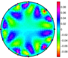
The forth column in Figure 2-3 shows the reconstructed images using tSVD pseudoinverse where is the number corresponding to and . Due to the change of singular values decay pattern, is close to the number of pixel . We will denote the corresponding reconstructed image by :
The fifth column in Figure 2-3 shows the reconstructed images using tSVD pseudoinverse :
The parameter is an weighting factor to balance between the LM and S-FM. In the special case of , the image of is similar to the image of . Here, we choose .
The choice of is more involved. Since we use a TSVD, our reconstruction lies inside a -dimensional space spanned by right singular vectors. Hence, it seems natural that an optimal choice of should be related to the number of pixels that belong to the inclusion. To estimate the number of pixels inside the inclusion we count the pixels in the S-FM reconstruction. More precisely, we take the number of pixels for which the S-FM-indicator value belongs to the upper third of the indicator values, and then, to be on the safe side, we double this number. Hence, the truncation number is chosen by
where is a number of elements of a set , and and . In the Figure 2-3, the set occupies a region of reddish part of image (not region of yellowish part).
4 Conclusion
We developed a modified discrete version of the factorization method (FM), herein called sensitivity matrix based FM(S-FM) that can be used as a regularization term for the standard linearized reconstruction method (LM). The S-FM provides a pixel-wise index indicating the possibility of the presence of anomaly at each pixel. Using this information for regularizing the LM resulted in an a better localization of anomalies and alleviated Gibbs ringing artifacts.
We should mention about the choice of in (28). Indeed, the choice is motivated by heuristical arguments and numerical evidence. The role of the augmented matrix is that the right singular vectors associated with high singular values are used to reconstruct images of anomaly region ( ). The choice of representing the unknown is somehow limited. Future studies will be concerned with rigorously justified ways of extending the linearized method with shape reconstruction properties.
References
- [1] A. Adler and W.R.B. Lionheart, Uses and abuses of EIDORS: An extensible software base for EIT, Physiol Meas. 27 (2006), pp. S25-42.
- [2] A. Adler A et al., GREIT: a unified approach to 2D linear EIT reconstruction of lung images, Physiol. Meas. 30 (2009), pp. S35-55.
- [3] D.C. Barber and B.H. Brown, Applied potential tomography, J. Phys. E: Sci. Instrum. 17 (1984), pp. 723-34.
- [4] J. Bikowski, K. Knudsen and J. L. Mueller, Direct numerical reconstruction of conductivities in three dimensions using scattering transforms, Inverse Problems 27 (2011), 015002.
- [5] L. Borcea, G. A. Gray and Y. Zhang, Variationally constrained numerical solution of electrical impedance tomography, Inverse Problems 19 (2003), pp. 1159-1184.
- [6] B.H. Brown and D.C. Barber, Electrical impedance tomography; the construction and application to physiological measurement of electrical impedance images, Med. Prog. Technol. 13 ( 1987), pp. 69-75.
- [7] B.H. Brown, D.C. Barber and A.D. Seagar, Applied potential tomography: possible clinical applications, Clin. Phys. Physiol. Meas. 6 (1985), pp. 109-21.
- [8] M. Brühl, Explicit characterization of inclusions in electrical impedance tomography, SIAM J. Math. Anal. 32 (2001), pp. 1327-41.
- [9] M. Brühl and M. Hanke, Numerical implementation of two noniterative methods for locating inclusions by impedance tomography, Inverse Problems 16 (2000), pp. 1029-42.
- [10] M. Cheney, D. Isaacson and J.C. Newell, Electrical impedance tomography, SIAM Rev. 41 (1999), pp. 85-101.
- [11] M. Cheney, D. Isaacson, J.C. Newell, S. Simske and J. Goble NOSER: An algorithm for solving the inverse conductivity problem, Int. J. Imag. Syst. Tech. 2 (1990), pp. 66-75.
- [12] H.W. Engl, M. Hanke and A. Neubauer, Regularization of inverse problems, Kluwer Academic Publishers, Boston, 2000.
- [13] B. Gebauer, Localized potentials in electrical impedance tomography, Inverse Probl. Imaging 2 (2008), pp. 251-269.
- [14] D.G. Gisser, D. Isaacson and J.C. Newell, Theory and performance of an adaptive current tomography system, Clin. Phys. Physiol. Meas. 9 (1988), pp. 35-41.
- [15] M. Hanke and M. Brühl, Recent progress in electrical impedance tomography, Inverse Problems 19 (2003). pp. S65-90.
- [16] M. Hanke, B. Harrach and N. Hyvönen, Justification of point electrode models in electrical impedance tomography, Math. Models Methods Appl. Sci. 21 (2011), pp. 1395-1413.
- [17] M. Hanke and A. Kirsch, Sampling methods, in O. Scherzer, editor, Handbook of Mathematical Models in Imaging, pp. 501–50. Springer, 2011.
- [18] B. Harrach and J.K. Seo, Detecting inclusions in electrical impedance tomography without reference measurements, SIAM J. Appl. Math. 69 (2009), pp. 1662–81.
- [19] B. Harrach and J.K. Seo, Exact shape-reconstruction by one-step linearization in electrical impedance tomography, SIAM J. Math. Anal. 42 (2010), pp. 1505-18.
- [20] B. Harrach, J.K. Seo and E.J. Woo, Factorization method and its physical justification in frequency-difference electrical impedance tomography, IEEE Trans. Med. Imag. 29 (2010), pp. 1918-26.
- [21] B. Harrach, Recent progress on the factorization method for electrical impedance tomography, to appear in Comput. Math. Methods Med.
- [22] D. Holder, Electrical impedance tomography: Methods, history and applications, Institute of Physics Publishing, Bristol, UK, D 2004.
- [23] D. Isaacson, Distinguishability of conductivities by electric current computed tomography, IEEE Trans. Med. Imag. 5 (1986), pp. 91-5.
- [24] D. Isaacson and M. Cheney, Effects of measurement precision and finite numbers of electrodes on linear impedance imaging algorithms, SIAM J. Appl. Math. 51 (1991), pp. 1705-31.
- [25] S.C. Jun, J. Kuen, J. Lee, E.J. Woo, D. Holder and J.K. Seo, Frequency-difference EIT (fdEIT) using weighted difference and equivalent homogeneous admittivity: validation by simulation and tank experiment, Physiol. Meas. 30 (2009), 1087-99.
- [26] A. Kirsch, Characterization of the shape of a scattering obstacle using the spectral data of the far field operator, Inverse Problems 14 (1998), pp. 1489-512.
- [27] A. Kirsch, An introduction to the mathematical theory of inverse problems, Springer, 2011.
- [28] A. Kirsch and N. Grinberg, The factorization method for inverse problem, Oxford Lecture Series in Mathematics and its Applications 36, Oxford University Press, 2008.
- [29] P. Metherall, D.C. Barber, R.H. Smallwood and B.H. Brown, Three dimensional electrical impedance tomography, Nature 380 (1996), pp. 509-12.
- [30] J.C. Newell, D.G. Gisser and D. Isaacson, An electric current tomograph, IEEE Trans. Biomed. Eng. 35 (1988), pp. 828-33.
- [31] A. Nachman, Global uniqueness for a two-dimensional inverse boundary value problem Ann. of Math. (2) 143 (1996), pp. 71-96.
- [32] R. G. Novikov, A multidimensional inverse spectral problem for the equation , (Russian) Funktsional. Anal. i Prilozhen. 22 (1988), 11-22, 96; translation in Funct. Anal. Appl. 22 (1989), pp. 263-272.
- [33] R. G. Novikov, An effectivization of the global reconstruction in the Gel’fand- Calderón inverse problem in three dimensions, Imaging microstructures, 161-184, Contemp. Math., 494, Amer. Math. Soc., Providence, RI, 2009.
- [34] J.G. Webster, An intelligent monitor for ambulatory ECGs, Biomed. Sci. Instrum. 14 (1978), pp. 55-60.
- [35] A. Wexler, B. Fry and M.R. Neuman, Impedance-computed tomography algorithm and system, Appl. Opt. 24 (1985), pp. 3985-92.
- [36] G.K. Wolf, B. Grychtol, I. Frerichs, H. van Genderingen, D. Zurakowski, E.J. Thompson and J.H. Arnold, Regional lung volume changes in children with acute respiratory distress syndrome during a derecruitment maneuver, Crit. Care Med. 35 (2007), pp. 1972-8.
- [37] T.J. Yorkey, J.G. Webster and W.J. Tompkins, Comparing reconstruction algorithms for electrical impedance tomography, IEEE Trans. Biomed. Eng. 34 (1987), pp. 843-52.