Majorana flat band edge modes of topological gapless phase in 2D Kitaev square lattice

Abstract

We study a Kitaev model on a square lattice, which describes topologically trivial superconductor when gap opens, while supports topological gapless phase when gap closes. The degeneracy points are characterized by two vortices in momentum space, with opposite winding numbers, which are not removable unless meet together. We show rigorously that the topological gapless phase always hosts a partial Majorana flat band edge modes in a ribbon geometry, although such a single band model has zero Chern number as a topologically trivial superconductor. The flat band disappears when the gapless phase becomes topologically trivial, associating with the mergence of two vortices. Numerical simulation indicates that the flat band is robust against the disorder. This finding indicates that the bulk-edge correspondence can be extended to superconductors in the topologically trivial regime as recently proposed in Ref. [PRL 118, 147003 (2017)].

Introduction

Topological materials have become the focus of intense research in the last years [1, 2, 3, 4], since they not only exhibit new physical phenomena with potential technological applications, but also provide a fertile ground for the discovery of fermionic particles and phenomena predicted in high-energy physics, including Majorana [5, 6, 7, 8, 9, 10], Dirac [11, 12, 13, 14, 15, 16, 17] and Weyl fermions [18, 19, 20, 21, 22, 23, 24, 25, 26]. These concepts relate to Majorana edge modes and topological gapless phases. System in the topological gapless phase exhibits band structures with band-touching points in the momentum space, where these kinds of nodal points appear as topological defects of an auxiliary vector field. Then these points are unremovable due to the symmetry protection, until a pair of them meets and annihilates together. On the other hand, a gapful phase can be topologically non-trivial, commonly referred to as topological insulators and superconductors, the band structure of which is characterized by nontrivial topology. A particularly important concept is the bulk-edge correspondence, which links the nontrivial topological invariant in the bulk to the localized edge modes. The number of Majorana edge modes is determined by bulk topological invariant. In general, edge states are the eigenstates of Hamiltonian that are exponentially localized at the boundary of the system. The Majorana edge modes have been actively pursued in condensed matter physics [27, 28, 29, 30, 31, 32, 33] since spatially separated Majorana fermions lead to degenerate ground states, which encode qubits immune to local decoherence [34].  This bulk-edge correspondence indicates that a single-band model must have vanishing Chern number and there should be no edge modes when open boundary conditions are applied. However, the existence of topological gapless indicates that there is hidden topological feature in some single band system. A typical system is a 2D honeycomb lattice of been graphene, which is a zero-band-gap semiconductor with a linear dispersion near the Dirac point. Meanwhile, there is another interesting feature lies in the appearance of partial flat band edge modes in a ribbon geometry [35, 36, 37], which exhibit robustness against disorder [38]. Recently, it has been pointed that Majorana zero modes are not only attributed to topological superconductors. A 2D topologically trivial superconductors without chiral edge modes can host robust Majorana zero modes in topological defects [39]. All these facts stimulate a question that the bulk-edge correspondence may be extended to a topological gapless phase.

In this paper, we investigate this issue through an exact solution of a concrete system. We study a Kitaev model on a square lattice, which describes topologically trivial superconductor when gap opens, while supports topological gapless phase when gap closes [40, 41]. The degeneracy points are characterized by two vortices, or Weyl nodal points in momentum space, with opposite winding numbers, which are not removable unless meet together. This work aims to shed light on the nature of topological edge modes associated with topological gapless phase, rather than gapful topological superconductor. We show rigorously that the topological gapless phase always hosts a partial Majorana flat band edge modes in a ribbon geometry. The flat band disappears when the gapless phase becomes topologically trivial, associating with the mergence of two vortices. Numerical simulation indicates that the flat band is robust against the disorder.

1 Results

We have demonstrated that a topologically trivial superconductor emerges as a topological gapless state, which support Majorana flat band edge modes. The new quantum state is characterized by two linear band-degeneracy points with opposite topological invariant. In sharp contrast to the conventional topological superconductor, such a system has single band, thus has zero Chern number. We prove that the appearance of this topological feature attributes to the corresponding Majorana lattice structure, which is a modified honeycomb lattice. It is natural to acquire a set of zero modes, which is robust against disorder. The results of our model indicate that the bulk-edge correspondence can be extended to a single-band system with hidden topological feature. In the following, there are three parts: (i) We present the Kitaev Hamiltonian on a square lattice and the phase diagram for the topological gapless phase. (ii) We investigate the Majorana bound states. (iii) We perform numerical simulation to investigate the robust of the edge modes against the disorder perturbations.

1.1 Model and topological gapless phase

We consider the Kitaev model on a square lattice which is employed to depict $2$D $p$-wave superconductors. The Hamiltonian of the tight-binding model reads

$$H = -t\sum_{\mathbf{r,a}}c_{\mathbf{r}}^{\dagger}c_{\mathbf{r}+\mathbf{a}}-\Delta\sum_{\mathbf{r},\mathbf{a}}c_{\mathbf{r}}c_{\mathbf{r}+\mathbf{a}}+\text{h.c.}$$ (1)

$$+\mu\sum_{\mathbf{r}}\left(2c_{\mathbf{r}}^{\dagger}c_{\mathbf{r}}-1\right),$$

where $\mathbf{r}$ is the coordinates of lattice sites and $c_{\mathbf{r}}$ is the fermion annihilation operators at site $\mathbf{r}$. Vectors $\mathbf{a}=a\mathbf{i},$ $a\mathbf{j},$ are the lattice vectors in the $x$ and $y$ directions with unitary vectors $\mathbf{i}$ and $\mathbf{j}$. The hopping between neighboring sites is described by the hopping amplitude $t$. The isotropic order parameter $\Delta$ is real, which result in topologically trivial superconductor. The last term gives the chemical potential.

Taking the Fourier transformation

$$c_{\mathbf{r}}=\frac{1}{N}\sum_{\mathbf{k}}c_{\mathbf{k}}e^{i\mathbf{k}\cdot\mathbf{r}},$$ (2)

the Hamiltonian with periodic boundary conditions on both directions can be rewritten as

$$H=\sum_{\mathbf{k}}\left(\begin{array}[]{cc}c_{\mathbf{k}}^{{\dagger}}&c_{-\mathbf{k}}\end{array}\right)h_{\mathbf{k}}\left(\begin{array}[]{c}c_{\mathbf{k}}\\ c_{-\mathbf{k}}^{{\dagger}}\end{array}\right),$$ (3)

where

$$h_{\mathbf{k}}=\left(\begin{array}[]{cc}\mu-t\cos k_{x}-t\cos k_{y}&i\Delta(\sin k_{x}+\sin k_{y})\\ -i\Delta(\sin k_{x}+\sin k_{y})&-\mu+t\cos k_{x}+t\cos k_{y}\end{array}\right),$$ (4)

where the summation of $\mathbf{k}=(k_{x},k_{y})$ is $\sum_{\mathbf{k}}=\sum_{k_{x}=-\pi}^{\pi}\sum_{k_{y}=-\pi}^{\pi}$. The core matrix can be expressed as

$$h_{\mathbf{k}}=\mathbf{B}\left(\mathbf{k}\right)\cdot\mathbf{\sigma},$$ (5)

where the components of the auxiliary field $\mathbf{B}\left(\mathbf{k}\right)=(B_{x},B_{y},B_{z})$ are

$$\left\{\begin{array}[]{c}B_{x}=0\\ B_{y}=-\Delta(\sin k_{x}+\sin k_{y})\\ B_{z}=\mu-t\cos k_{x}-t\cos k_{y}\end{array}\right..$$ (6)

$\mathbf{\sigma}$ are the Pauli matrices

$$\sigma_{x}=\left(\begin{array}[]{cc}0&1\\ 1&0\end{array}\right),\sigma_{y}=\left(\begin{array}[]{cc}0&-i\\ i&0\end{array}\right),\sigma_{z}=\left(\begin{array}[]{cc}1&0\\ 0&-1\end{array}\right).$$ (7)

The Bogoliubov spectrum is

$$\varepsilon_{\mathbf{k}} = \left|\mathbf{B}\left(\mathbf{k}\right)\right|$$ (8)

$$= 2\sqrt{\left[\mu-t\left(\cos k_{x}+\cos k_{y}\right)\right]^{2}+\Delta^{2}\left(\sin k_{x}+\sin k_{y}\right)^{2}}.$$

We are interested in the gapless state arising from the band touching point of the spectrum. The band degenerate point $\mathbf{k}_{0}=(k_{0x},k_{0y})$ is determined by

$$\left\{\begin{array}[]{l}-\Delta\left(\sin k_{0x}+\sin k_{0y}\right)=0,\\ \mu-t\left(\cos k_{0x}+\cos k_{0y}\right)=0.\end{array}\right.$$ (9)

As pointed in Ref. [40], two bands touch at three types of configurations: single point, double points, and curves in the $k_{x}$-$k_{y}$ plane, determined by the region of parameter $\Delta$-$\mu$ plane (in units of $t$). We focus on the non-trivial case with nonzero $\Delta$. Then we have

$$k_{0x}=-k_{0y}=\pm\arccos(\frac{\mu}{2t})$$ (10)

in the region $\left|\mu/t\right|\leqslant 2$, which indicates that there are two nodal points for $\mu\neq 0$ and $\left|\mu/t\right|\neq 2$. The two points move along the line represented by the equation $k_{0x}=-k_{0y}$, and merge at $\mathbf{k}_{0}=(\pi,-\pi)$ when $\mu/t=\pm 2$. In the case of $\mu=0$, the nodal points become two nodal lines represented by the equations $k_{0y}$ $=$ $\pm\pi+k_{0x}$. The phase diagram is illustrated in Fig. 1, depending on the values of $\mu$ and $\Delta$ (compared with the hopping strength $t$). We plot the band structures in Fig. 2 and Fig. 3 for several typical cases.

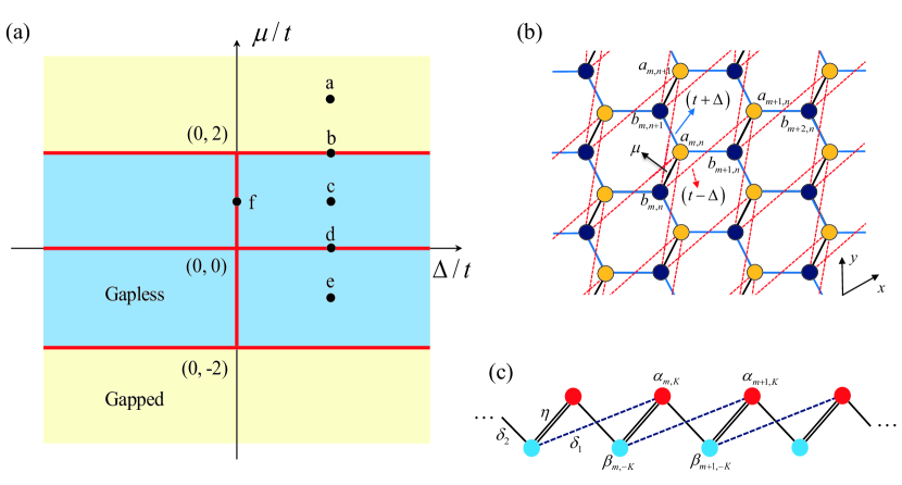
Figure 1: (Color online) (a) Phase diagram of the Kitaev model on a square lattice system on the parameter $\mu-\Delta$ plane (in units of $t$). The red lines indicate the boundary, which separate the topologically trivial gapped phases (yellow) and topological gapless phases (blue). The system at the boundary (red lines) is topologically trivial gapless phase. (b) Schematically illustration of the Majorana lattice, which is honeycomb geometry with long-range hopping term. (c) The geometry of the auxiliary operator lattice represented in Eq. (22), which is an SSH chain with long-range hopping term. The edge modes of a set of modified SSH chains form Majorana fat band edge modes in (b) when the system is in the blue region of the phase diagram (a).

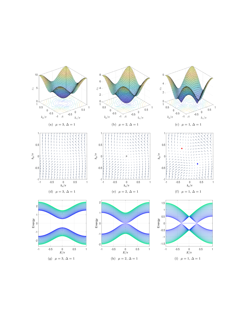
Figure 2: (Color online) (a)-(c) Plots of energy spectra from Eq. (8) at three typical points a, b, and c marked in the phase diagram in Fig. 1.. There is gapped in (a), a single degeneracy point with parabolic dispersion in (b), and two degeneracy points with linear dispersion in (c). (d)-(f) Plots of field defined in Eq. (6) in the momentum space for three cases corresponding to (a)-(c). There are two vortices in (f) with opposite winding numbers $\pm 1$. As $\mu$ increases, two vortices close and merge into a single point in (e). As $\mu$ increases to 3, the field become trivial in (d). (g)-(i) Plots of the spectra from Eq. (21) with $M=40$ for three cases of (a)-(c). It indicates that the existence of pair of vortices links to a flat band of Majorana lattice.

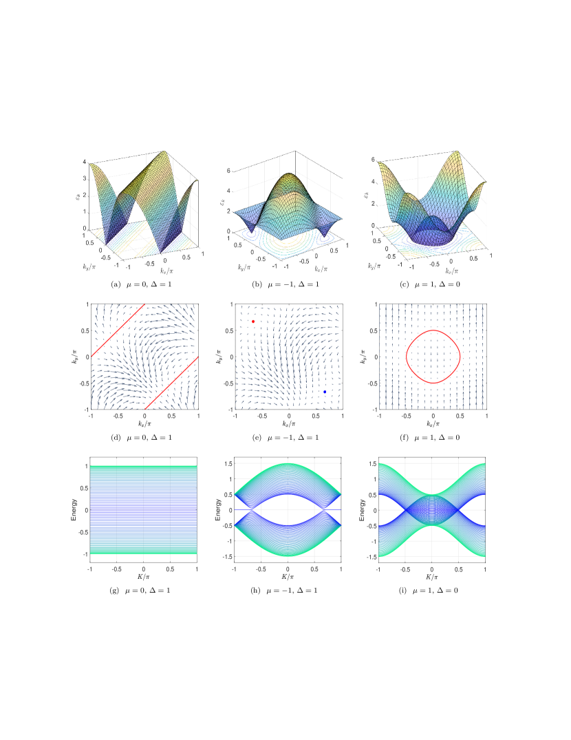
Figure 3: (Color online) (a)-(c) Plots of energy spectra from Eq. (8) at three typical points d, e, and f marked in the phase diagram in Fig. 1.. There is two degeneracy lines in (a), two degeneracy points with linear dispersion in (b), and a degeneracy loop in (c). (d)-(f) Plots of field defined in Eq. (6) in the momentum space for three cases corresponding to (a)-(c). There are two vortices in (e) with opposite winding numbers $\pm 1$. (g)-(i) Plots of the spectra from Eq. (21) with $M=40$ for three cases of (a)-(c). It indicates that the existence of pair of vortices links to a flat band of Majorana lattice.

In the vicinity of the degeneracy points, we have

$$\left\{\begin{array}[]{l}B_{x}=0\\ B_{y}=-\Delta\cos k_{0x}\left(q_{y}+q_{x}\right)\\ B_{z}=t\sin k_{0x}\left(q_{x}-q_{y}\right)\end{array}\right.,$$ (11)

where $\mathbf{q=k-k}_{0}$, $\mathbf{k}_{0}=\left(k_{0x},k_{0y}\right)$ and $\left(k_{0x},k_{0y}\right)$ satisfy Eq. (10), is the momentum in another frame. Around these degeneracy points, the Hamiltonian $h_{\mathbf{k}}$ can be linearized as the form

$$\mathcal{H}(\mathbf{q})=\sum_{i,j}a_{ij}q_{i}\sigma_{j},$$ (12)

which is equivalent to the Hamiltonian for two-dimensional massless relativistic fermions. Here $\left(q_{1},q_{2}\right)=\left(q_{x},q_{y}\right)$ and $\left(\sigma_{1},\sigma_{2}\right)=\left(\sigma_{y},\sigma_{z}\right)$. The corresponding chirality for these particle is defined as

$$w=\mathrm{sgn}[\det(a_{ij})].$$ (13)

Then we have

$$\det\left|\begin{array}[]{cc}-\Delta\cos k_{0x}&t\sin k_{0x}\\ -\Delta\cos k_{0x}&-t\sin k_{0x}\end{array}\right|=t\Delta\sin 2k_{0x},$$ (14)

which leads to $w=\pm 1$ for two nodal points. The chiral relativistic fermions serve as two-dimensional Weyl fermions. Two Weyl nodes located at two separated degenerate points have opposite chirality. We note that for $\Delta\left|\mu/t\right|(\left|\mu/t\right|-2)=0$, we have $w=0$. At this situation, two Weyl nodes merge at $(0,0)$ and $(\pm\pi,\mp\pi)$. The topology of the nodal point becomes trivial, and a perturbation hence can open up the energy gap. We illustrate the vortex structure of the degeneracy point in $k_{x}$-$k_{y}$ plane in Fig. 2 and Fig. 3. As shown in figures, we find three types of topological configurations: pair of vortices with opposite chirality, single trivial vortex (or degeneracy lines), and no vortex, corresponding to topological gapless, trivial gapless and gapped phases, respectively.

1.2 Majorana flat band edge modes

Now we turn to study the feature of gapless phase in the framework of Majorana representation. The Kitaev model on a honeycomb lattice and chain provides well-known examples of systems with such a bulk-boundary correspondence [43, 44, 45, 46, 47, 48, 49]. It is well known that a sufficient long chain has Majorana modes at its two ends [50]. A number of experimental realizations of such models have found evidence for such Majorana modes [7, 51, 52, 53, 54]. In contrast to previous studies based on a gapful system with nonzero Chern number, we focus on the Kitaev model in the topologically trivial phase. This is motivated by the desire to get a connection between the Majorana edge modes and topological nature hidden in a topologically trivial superconductor. At first, we revisit the description of the present model on a cylindrical lattice in terms of Majorana fermions.

We introduce Majorana fermion operators

$$a_{\mathbf{r}}=c_{\mathbf{r}}^{\dagger}+c_{\mathbf{r}},b_{\mathbf{r}}=-i\left(c_{\mathbf{r}}^{\dagger}-c_{\mathbf{r}}\right),$$ (15)

which satisfy the relations

$$\left\{a_{\mathbf{r}},a_{\mathbf{r}^{\prime}}\right\} = 2\delta_{\mathbf{r},\mathbf{r}^{\prime}},\left\{b_{\mathbf{r}},b_{\mathbf{r}^{\prime}}\right\}=2\delta_{\mathbf{r},\mathbf{r}^{\prime}},$$

$$\left\{a_{\mathbf{r}},b_{\mathbf{r}^{\prime}}\right\} = 0,a_{\mathbf{r}}^{2}=b_{\mathbf{r}}^{2}=1.$$ (16)

Then the Majorana representation of the Hamiltonian is

$$H = \frac{1}{4}\sum_{\mathbf{r}}[i(t+\Delta)\sum_{\mathbf{a}}a_{\mathbf{r}}b_{\mathbf{r+a}}$$ (17)

$$+i(t-\Delta)\sum_{\mathbf{a}}a_{\mathbf{r+a}}b_{\mathbf{r}}-i2\mu a_{\mathbf{r}}b_{\mathbf{r}}+\text{{h.c.}}].$$

It represents a honeycomb lattice with extra hopping term $a_{\mathbf{r+a}}b_{\mathbf{r}}$, which is schematically illustrated in Fig. 1. Before a general investigation, we consider a simple case to show that a flat band Majorana modes do exist. Taking $t=\Delta=\mu$ the Hamiltonian reduces to

$$H_{\text{hc}}=\frac{t}{2}\sum_{\mathbf{r}}(ia_{\mathbf{r}}\sum_{\mathbf{a}}b_{\mathbf{r+a}}-ia_{\mathbf{r}}b_{\mathbf{r}}+\text{{h.c.}}).$$ (18)

which corresponds to a honeycomb ribbon with zigzag boundary condition. It is well-known that there exist a partial flat band edge modes in such a lattice system[35, 36, 37, 38].

In the following, we will show that this feature still remains in a wide parameter region. Consider the lattice system on a cylindrical geometry by taking the periodic boundary condition in one direction and open boundary in another direction. For a $M\times M$ Kitaev model, the Majorana Hamiltonian can be explicitly expressed as

$$H_{\text{M}} = \frac{i}{4}\sum_{l,j=1}^{M}[(t-\Delta)(a_{m,n+1}b_{m,n}+a_{m+1,n}b_{m,n})$$ (19)

$$+(t+\Delta)(a_{m,n}b_{m,n+1}+a_{m,n}b_{m+1,n})-2\mu a_{m,n}b_{m,n}-\mathrm{h.c.}],$$

by taking $\mathbf{r=}m\mathbf{i+}n\mathbf{j}\rightarrow(m,n)$. The boundary conditions are $a_{n,1}=a_{n,M+1}$, $b_{n,1}=b_{n,M+1}$, $a_{M+1,n}=0$, and $b_{M+1,n}=0$.

Consider the Fourier transformations of Majorana operators

$$\left\{\begin{array}[]{c}\alpha_{m,K}=\frac{1}{\sqrt{N}}\sum_{n=1}^{M}e^{-iKn}a_{m,n}\\ \beta_{m,K}=\frac{1}{\sqrt{N}}\sum_{n=1}^{M}e^{-iKn}b_{m,n}\end{array}\right.,$$ (20)

where the wave vector $K=2\pi l/N$, $l=1,2,...,N$.

The Hamiltonian $H_{\text{M}}$ can be rewritten as

$$H_{\text{M}} = \sum_{K}h_{\text{M}}^{K},$$ (21)

$$h_{\text{M}}^{K} = \sum_{m=1}^{M-1}(\eta\alpha_{m,K}i\beta_{m,-K}+\delta_{1}\alpha_{m+1,K}i\beta_{m,-K}$$ (22)

$$+\delta_{2}\alpha_{m,K}i\beta_{m+1,-K})+\eta\alpha_{M,K}i\beta_{M,-K}+\mathrm{h.c.,}$$

where $\eta=[(t-\Delta)e^{iK}+(t+\Delta)e^{-iK}-2\mu]/4$, $\delta_{1}=(t-\Delta)/4$ and $\delta_{2}=(t+\Delta)/4$, and $h_{\text{M}}^{K}$ obeys

$$[h_{\text{M}}^{K},h_{\text{M}}^{K^{\prime}}]=0,$$ (23)

i.e., $H_{\text{M}}$ has been block diagonalized. We would like to point that operators $\alpha_{m,K}$ and$\ \beta_{m,K}$ are not Majorana fermion operators except the cases with $K=0$ or $\pi$. We refer such operators as to auxiliary operators. We note that each $h_{\text{M}}^{K}$ represents a modified SSH chain about auxiliary operators $\alpha_{m,K}$ and$\ \beta_{m,K}$ with $\eta$, $\delta_{1}$, and $\delta_{2}$ hopping terms. One can always get a diagonalized $h_{\text{M}}^{K}$ through the diagonalization of the matrix of the corresponding single-particle modified SSH chain. For simplicity, we only consider the case with positive parameters $t,$ $\Delta,$ and $\mu$. In large $M$ limit, there are two zero modes for $h_{\text{M}}^{K}$ under the condition $0<\mu<2$ (in units of $t$). Actually, it can be checked that $h_{\text{M}}^{K}$ can contribute a term

$$0\times(\gamma_{K}^{{\dagger}}\gamma_{K}-\gamma_{K}\gamma_{K}^{{\dagger}}),$$ (24)

where

$$\gamma_{K}=A\sum_{j=1}^{M}\left[\left(p_{+}^{M-j+1}-p_{-}^{M-j+1}\right)\alpha_{j,K}+i\left(p_{+}^{j}-p_{-}^{j}\right)\beta_{j,K}\right].$$ (25)

Here $A=\left(2\sum_{j=1}^{M}\left|p_{+}^{j}-p_{-}^{j}\right|^{2}\right)^{-\frac{1}{2}}$ is normalization constant, and

$$p_{\pm}=\frac{\pm\sqrt{\left|\eta\right|^{2}-4\delta_{1}\delta_{2}}-\left|\eta\right|}{2\delta_{2}}.$$ (26)

The term in Eq. (24) exists under the convergence condition

$$\lim_{j\rightarrow\infty}\left(p_{+}^{j}-p_{-}^{j}\right)=0\mathbf{.}$$ (27)

As expected, we note that operators $\gamma_{K}$ satisfy the fermion commutation relations

$$\left\{\gamma_{K},\gamma_{K^{\prime}}^{{\dagger}}\right\}=2\delta_{KK^{\prime}},\left\{\gamma_{K},\gamma_{K^{\prime}}\right\}=0,$$ (28)

representing edge modes. The sufficient condition for Eq. (27) is

$$\left|p_{\pm}\right|<1,$$ (29)

which leads to

$$\left\{\begin{array}[]{c}\left|\eta\right|<2\left|\delta_{2}\right|\\ -\left|\delta_{2}\right|^{2}+\left|\eta\delta_{2}\right|<\delta_{1}\delta_{2}\leqslant\left|\frac{\eta}{2}\right|^{2}\end{array}\right.,$$ (30)

or more explicitly form

$$\left\{\begin{array}[]{l}R-2t\Delta<0\\ \Delta^{2}>R+2\Delta^{2}\geqslant 0\end{array}\right.,$$ (31)

where $R\left(K,\Delta,\mu,t\right)=(t^{2}-\Delta^{2})\cos^{2}(K)-2\mu t\cos(K)+\mu^{2}-t^{2}$. To demonstrate this result, considering a simple case with $\Delta=\mu=t,$ we find that $R$ reduces to $-2\Delta^{2}\cos(K)$ and satisfies above equations when take $-\pi/3<K<\pi/3$. Furthermore the parameters become $\eta=\Delta(e^{-iK}-1)/2$, $\delta_{1}=0$ and $\delta_{2}=\Delta/2$, and $h_{\text{M}}^{K}$ corresponds to a simple SSH chain with $\left|\eta\right|<\left|\delta_{2}\right|$. The edge mode wave functions can be obtained from $p_{+}=0$ and $p_{-}=-\sqrt{2\left(1-\cos K\right)}$. Then the existence of edge modes is well reasonable. The zero modes in the plot of energy band in Fig. 2(i) corresponds this flat band of edge mode.

1.3 Disorder perturbation

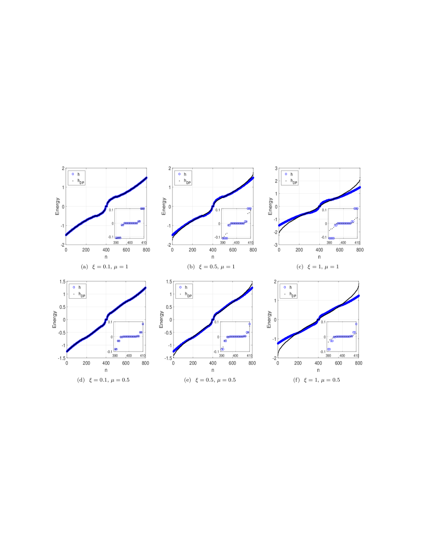
Figure 4: (Color online) Plots of eigenvalues of matrices $h$ and $h_{\text{DP}}$ with typical parameters and different disorder strength factor $\xi$. The dimension of matrix is $800$, corresponding to $M=20$. According to analytical analysis, there are $10$ and $14$ quasi-zero modes in the upper and lower panels. Here we take $\Delta=t=1$. Numerical results show that as $\xi$ increases, most of levels of $h_{\text{DP}}$ deviate from that of $h$, while the zero-mode levels remain unchanged, indicating the robustness of zero modes against to the disorder.

One of the most striking features of topologically protected edge states is the robustness against to certain types of disorder perturbation to the original Hamiltonian. In this section, we investigate the robustness of the Majorana edge flat band in the presence of disorder. The disorder we discuss here arises from the parameters $\left\{t,\Delta,\mu\right\}$ in the Hamiltonian $H_{\text{M}}$. More precisely, one can rewrite the Hamiltonian in the form

$$H_{\text{M}}=\psi^{{\dagger}}h\psi,$$ (32)

where $h$ represents a $2M^{2}\times 2M^{2}$ matrix in the basis

$$\psi = (a_{1,1},ib_{1,1},...,a_{1,M},ib_{1,M},$$ (33)

$$a_{2,1},ib_{2,1},...,a_{2,M},ib_{2,M},$$

$$...,a_{i,j},ib_{i,j},...,$$

$$a_{M,1},ib_{M,1},...,a_{M,M},ib_{M,M})^{T}.$$

We introduce the disorder perturbation to $H_{\text{M}}$ by preserving the time reversal symmetry, i.e., keeping the reality of the parameters $\left\{t,\Delta,\mu\right\}$. We take the randomized matrix elements in $h$ by the replacement

$$\left\{\begin{array}[]{c}t\rightarrow t_{l.j}=r_{l,j}^{a}t\\ \Delta\rightarrow\Delta_{l.j}=r_{l,j}^{b}\Delta\\ \mu\rightarrow\mu_{l.j}=r_{l,j}^{c}\mu\end{array}\right.,$$ (34)

to get the disorder matrix $h_{\text{DP}}$. Here $r^{a,b,c}$ are three $M\times M$ matrices which consist of random numbers in the interval of $\left(1-\xi,1+\xi\right)$, influencing each matrix elements. Real factor $\xi$ plays the role of the disorder strength.

We investigate the influence of nonzero $\xi$ by comparing two sets of eigenvalues obtained by numerical diagonalization of finite-dimensional matrices $h$ and $h_{\text{DP}}$, respectively. The plots in Fig. 4. indicate that the zero modes remain unchanged in the presence of random perturbations with not too large $\xi$. The numerical result support our conclusion that the topological gapless states correspond to the presence of topologically protected edge modes.

2 Discussion

According to the bulk-edge correspondence, it seems that the existence of edge states requires a gapped topological phase. This may not include the case with a single band which contains topological gapless states. The topological character of a gapless state does not require the existence of the gap. This arises the question: What is the essential reason for the edge state, energy gap or topology of the energy band? Obviously, energy gap is not since many gapped systems do not support the edge states. Then it is possible that a special single band system supports the edge states. In the case of the lack of an exact proof, concrete example is desirable. As such an example we have considered a Kitaev model on a square lattice, which describes topologically trivial superconductor when gap opens, while supports topological gapless phase when gap closes. The degeneracy points are characterized by two vortices, or Weyl nodal points in momentum space, with opposite winding numbers, which are not removable unless meet together. We demonstrated that a topologically trivial superconductor emerges as a topological gapless state, which support Majorana flat band edge modes. The new quantum state is characterized by two linear band-degeneracy points with opposite topological invariant. In sharp contrast to the conventional topological superconductor, such a system has single band, thus has zero Chern number. We prove that the appearance of this topological feature attributes to the corresponding Majorana lattice structure, which is a modified honeycomb lattice. The topological feature of an edge state is the robustness against disorder. The numerical results indicate that such a criteria is met for this concrete example. We also note that the topological gapless state and the edge state have the same energy level, which is also an open question in the future.

Author contributions statement

Z.S. conceived the idea and carried out the study. K.L.Z, P.W. and Z.S. discussed the results. Z.S and K.L.Z wrote the manuscript with inputs from all the other authors.

Additional information

Competing interests: The authors declare no competing interests.

References

- [1] Hasan, M. Z. & Kane, C. L. Colloquium: Topological insulators. Rev. Mod. Phys. 82, 3045-3067 (2010).
- [2] Qi, X. L. & Zhang, S. C. Topological insulators and superconductors. Rev. Mod. Phys. 83, 1057-1110 (2011).
- [3] Chiu, C. K., Teo, J. C. Y., Schnyder, A. P. & Ryu, S. Classification of topological quantum matter with symmetries. Rev. Mod. Phys. 88, 035005 (2016).
- [4] Weng, H., Yu, R., Hu, X., Dai, X. & Fang, Z. Quantum anomalous Hall effect and related topological electronic states. Adv. Phys. 64, 227–282 (2015).
- [5] Fu, L. & Kane, C. L. Superconducting Proximity Effect and Majorana Fermions at the Surface of a Topological Insulator. Phys. Rev. Lett. 100, 096407 (2008).
- [6] Lutchyn, R. M., Sau, J. D. & Sarma, S. Das. Majorana Fermions and a Topological Phase Transition in Semiconductor-Superconductor Heterostructures. Phys. Rev. Lett. 105, 077001 (2010).
- [7] Mourik, V. et al. Signatures of Majorana Fermions in Hybrid Superconductor-Semiconductor Nanowire Devices. Science 336, 1003 (2012).
- [8] Nadj-Perge, S. et al. Observation of Majorana fermions in ferromagnetic atomic chains on a superconductor. Science 346 602 (2014).
- [9] Oreg, Y., Refael, G. & Oppen, F. von. Helical Liquids and Majorana Bound States in Quantum Wires. Phys. Rev. Lett. 105, 177002 (2010).
- [10] Read, N. & Green, D. Paired states of fermions in two dimensions with breaking of parity and time-reversal symmetries and the fractional quantum Hall effect. Phys. Rev. B 61, 10267 (2000).
- [11] Neto, A. H. C., Guinea, F., Peres, N. M. R., Novoselov, K. S. & Geim, A. K. The electronic properties of graphene. Rev. Mod. Phys. 81, 109 (2009).
- [12] Liu, Z. K. et al. A stable three-dimensional topological Dirac semimetal CdAs. Nat. Mater. 13, 677–681 (2014).
- [13] Liu, Z. K. et al. Discovery of a Three-Dimensional Topological Dirac Semimetal, Na3Bi. Science 343, 864 (2014).
- [14] Steinberg, J. A. et al. Bulk Dirac Points in Distorted Spinels. Phys. Rev. Lett. 112, 036403 (2014).
- [15] Wang, Z. J. et al. Dirac semimetal and topological phase transitions in ABi(A=Na, K, Rb). Phys. Rev. B 85, 195320 (2012).
- [16] Xiong, J. et al. Evidence for the chiral anomaly in the dirac semimetal NaBi. Science 350, 413–416 (2015).
- [17] Young, S. M. et al. Dirac Semimetal in Three Dimensions. Phys. Rev. Lett. 108, 140405 (2012).
- [18] Hirschberger, M. et al. The chiral anomaly and thermopower of Weyl fermions in the half-Heusler GdPtBi. Nat. Mater. 15, 1161–1165 (2016).
- [19] Huang, S. M. et al. An inversion breaking Weyl semimetal state in the TaAs material class. Nat. Commun. 6, 7373 (2015).
- [20] Lv, B. Q. et al. Experimental Discovery of Weyl Semimetal TaAs. Phys. Rev. X 5, 031013 (2015).
- [21] Lv, B. Q. et al. Observation of Weyl nodes in TaAs. Nat. Phys. 11, 724–727 (2015).
- [22] Shekhar, C. et al. Observation of chiral magneto-transport in RPtBi topological Heusler compounds. arXiv:1604.01641.
- [23] Wan, X., Turner, A. M., Vishwanath, A. & Savrasov. S. Y. Topological semimetal and Fermi-arc surface states in the electronic structure of pyrochlore iridates. Phys. Rev. B 83, 205101 (2011).
- [24] Weng, H., Fang, C., Fang, Z., Bernevig, B. A. & Dai, X. Weyl Semimetal Phase in Noncentrosymmetric Transition-Metal Monophosphides. Phys. Rev. X 5, 011029 (2015).
- [25] Xu, S. Y. et al. Discovery of Weyl semimetal NbAs. Nat. Phys. 11, 748–754 (2015).
- [26] Xu, S. Y. et al. Discovery of a Weyl fermion semimetal and topological Fermi arcs. Science 349, 613-617 (2015).
- [27] Alicea, New directions in the pursuit of Majorana fermions in solid state systems. J., Rep. Prog. Phys. 75, 076501 (2012).
- [28] Beenakker, C. W. J. Search for Majorana Fermions in Superconductors. Annu. Rev. Condens. Matter Phys. 4, 113-136 (2013).
- [29] Stanescu, T. D. & Tewari, S. Majorana fermions in semiconductor nanowires: fundamentals, modeling, and experiment. J. Phys. Condens. Matter 25, 233201 (2013).
- [30] Leijnse, M. & Flensberg, K. Introduction to topological superconductivity and Majorana fermions. Semicond. Sci. Technol. 27 , 124003 (2012).
- [31] Elliott, S. R. & Franz, M. Colloquium: Majorana fermions in nuclear, particle, and solid-state physics. Rev. Mod. Phys. 87, 137 (2015).
- [32] Das Sarma, S., Freedman, M. & Nayak, C. Majorana Zero Modes and Topological Quantum Computation. NPJ Quantum Information 1, 15001 (2015).
- [33] Sato, M. & Fujimoto, S. Majorana Fermions and Topology in Superconductors. J. Phys. Soc. Jpn. 85, 072001 (2016).
- [34] Nayak, C., Simon, S. H., Stern, A., Freedman, M. & Das Sarma, S. Non-Abelian anyons and topological quantum computation. Rev. Mod. Phys. 80, 1083 (2008).
- [35] Fujita, M., Wakabayashi, K., Nakada, K. & Kusakabe, K. Peculiar Localized State at Zigzag Graphite Edge. J. Phys. Soc. Jpn. 65, 1920 (1996)
- [36] Ryu, S. & Hatsugai, Y. Topological Origin of Zero-Energy Edge States in Particle-Hole Symmetric Systems. Phys. Rev. Lett. 89, 077002 (2002)
- [37] Yao, W., Yang, S. A. & Niu, Q. Edge States in Graphene: From Gapped Flat-Band to Gapless Chiral Modes. Phys. Rev. Lett. 102, 096801 (2009)
- [38] Wakabayashi, K., Takane, Y. & Sigrist, M. Perfectly Conducting Channel and Universality Crossover in Disordered Graphene Nanoribbons. Phys. Rev. Lett. 99, 036601 (2007)
- [39] Yan, Z. B., Bi, R & Wang, Z. Majorana Zero Modes Protected by a Hopf Invariant in Topologically Trivial Superconductors. Phys. Rev. Lett. 118, 147003 (2017).
- [40] Wang, P., Lin, S., Zhang, G. & Song, Z. Topological gapless phase in Kitaev model on square lattice. Sci. Rep. 7, 17179 (2017).
- [41] Wang, P., Lin, S., Zhang, G. & Song, Z. Maximal distant entanglement in Kitaev tube. Sci. Rep. 8, 12202 (2018).
- [42] Hou, J. M. Hidden-Symmetry-Protected Topological Semimetals on a Square Lattice. Phys. Rev. Lett. 111, 130403 (2013)
- [43] Kitaev, A. Anyons in an exactly solved model and beyond. Ann. Phys. 321, 2 (2006).
- [44] Baskaran, G., Mandal, S. & Shankar, R. Exact Results for Spin Dynamics and Fractionalization in the Kitaev Model. Phys. Rev. Lett. 98, 247201 (2007)
- [45] Lee, D. H., Zhang, G. M. & Xiang, T. Edge Solitons of Topological Insulators and Fractionalized Quasiparticles in Two Dimensions. Phys. Rev. Lett. 99, 196805 (2007)
- [46] Schmidt, K. P., Dusuel, S. & Vidal, J. Emergent Fermions and Anyons in the Kitaev Model. Phys. Rev. Lett. 100, 057208 (2008).
- [47] Kells, G., Bolukbasi, A. T., Lahtinen, V., Slingerland, J. K., Pachos, J. K. & Vala, J. Topological Degeneracy and Vortex Manipulation in Kitaev’s Honeycomb Model. Phys. Rev. Lett. 101, 240404 (2008)
- [48] Kells, G., Slingerland, J. K. & Vala, J. Description of Kitaev’s honeycomb model with toric-code stabilizers. Phys. Rev. B 80 , 125415 (2009).
- [49] Kells, G. & Vala, J. Zero energy and chiral edge modes in a p-wave magnetic spin model. Phys. Rev. B 82, 125122 (2010)
- [50] Kitaev, A. Y. Unpaired Majorana fermions in quantum wires. Physics-Uspekhi 44, 131 (2001).
- [51] Rokhinson, L. P., Liu, X. & Furdyna, J. K. Observation of the fractional ac Josephson effect: the signature of Majorana particles. Nat. Phys. 8, 795 (2012).
- [52] Das, A., Ronen, Y., Most, Y., Oreg, Y., Heiblum, M. & Shtrikman, H. Evidence of Majorana fermions in an Al - InAs nanowire topological superconductor. Nat. Phys. 8, 887 (2012).
- [53] Finck, A. D. K., Van Harlingen, D. J., Mohseni, P. K., Jung, K. & Li, X. Anomalous Modulation of a Zero-Bias Peak in a Hybrid Nanowire-Superconductor Device. Phys. Rev. Lett. 110, 126406 (2013).
- [54] Banerjee, A., Bridges, C. A., Yan, J. Q. et al. Proximate Kitaev Quantum Spin Liquid Behaviour in . Nature Materials. 15, 733 (2016).
- [55] Lin, S., Zhang, G., Li, C. & Song, Z. Magnetic-flux-driven topological quantum phase transition and manipulation of perfect edge states in graphene tube. Sci. Rep. 6, 31953 (2016).
- [56] Yan, Z. B., Song, F. & Wang, Z. Majorana Corner Modes in a High-Temperature Platform. Phys. Rev. Lett. 121, 096803 (2018).
- [57] Wang, Q. Y., Liu, C. C., Lu, Y. M. & Zhang, F. High-Temperature Majorana Corner States. arXiv:1804.04711.
Acknowledgements
This work was supported by National Natural Science Foundation of China (under Grant No. 11874225).