TRANSFER LEARNING USING CLASSIFICATION LAYER FEATURES OF CNN

Abstract

Although CNNs have gained the ability to transfer learned knowledge from source task to target task by virtue of large annotated datasets but consume huge processing time to fine-tune without GPU. In this paper, we propose a new computationally efficient transfer learning approach using classification layer features of pre-trained CNNs by appending layer after existing classification layer. We demonstrate that fine-tuning of the appended layer with existing classification layer for new task converges much faster than baseline and in average outperforms baseline classification accuracy. Furthermore, we execute thorough experiments to examine the influence of quantity, similarity, and dissimilarity of training sets in our classification outcomes to demonstrate transferability of classification layer features.

Index Terms—  Transfer learning, deep networks, computational efficiency, classification

1 Introduction

The advancement of influential internal representations in human infancy is reused later in life to solve various problems as stated by the cognitive study of [1]. In resemblance to humans, deep neural networks built for computer vision problems also learn the data representations (features) which they use later to solve multiple tasks. This phenomenon of transferability of learned data representations is termed as transfer learning [2, 3, 4]. This technique works well when the learned features are generic, which refers to having features suitable to both base and target datasets. The opportunity to learn generic features for deep networks is paved by the ImageNet [5] dataset. Deep neural networks incline to learn generic features in the first layer that resemble Gabor filters and colour blobs irrespective of datasets and training objectives [6, 7, 8]. A number of works in various computer vision tasks have reported significant results by transferring inner layer features of deep networks [9, 10, 11]. As the deep network architecture moves toward fully-connected (FC) layers, the specificity increases while the generic nature of features decrease [12], i.e., the intuition is that they are highly specific to pre-trained classes and might not generalize well in transferring knowledge.

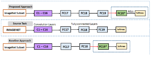
Fig. 1: Both proposed and baseline approach of transfer learning with corresponding source task are shown for VGG19 network architecture

However, a recent research by [13] demonstrated CNN architectures either by adding FC layers in between final FC layer and classification layer or by widening existing FC layers which outperformed classic fine-tuned transfer learning. They have used step wise hyper-parameters to keep pace with training time constraints. Motivated by their findings, we hypothesize to append new FC layer after existing classification layer (e.g. FC19 for VGG19) as shown in Fig.1. Eventually, we fine-tune new and existing classification layer to investigate that proposed approach consumes less training time because of having only 1000 dimensional feature vectors. In addition, do not adversely affect classification accuracy. Performance of proposed approach is compared with an existing approach which replaces the final FC layer with the number of new classes and fine-tune penultimate layer consisting 4096 or higher feature vectors along with the replaced one. Furthermore, we systematically investigate the following research questions (RQ) to study the impact of training sets in both proposed and baseline approaches. Eventually, demonstrate that classification layer features have similar behaviour as other FC layers for transfer learning.

RQ1: Does similarity of new classes with the pre-trained classes influence performance of classification using transfer learning?

RQ2: Does similarity among new classes influence the performance of classification using transfer learning?

RQ3: How much the performance of classification using transfer learning is influenced by the number of training and validation images used for new classes?

RQ4: How much the performance of classification using transfer learning is influenced when a mixed types of new classes are trained?

RQ5: Can proposed approach be used to improve computational efficiency without adversely affecting the performance of classification?

2 Related Work

A significant number of papers have experimented and studied transfer learning in CNNs, which includes various factors affecting fine-tuning, pre-training and freezing layers. Apparently, it has become a trend for computer vision community to treat convolutional neural networks [6, 14, 15, 16, 17] trained on ImageNet as extractors of features that can be reused in handling visualization tasks. Discussion on whether to stop pre-training early to avoid overfitting and which layers would be best transferable for transfer learning is studied by [18, 12]. [19] have investigated transfer learning based on noisy data. Fine-tune for new tasks without forgetting the old ones is proposed by [20]. To limit the need for annotated data required for transfer learning, [21] has proposed a method of more universal representations. The nature of transfer learning with mid-level features is studied by [22]. CNN features were used as off-the-shelf features by [23]. CNN features pre-trained in road scenes were reused for more specific road scene classifications by [24].
In this paper, we propose a transfer learning approach using pre-trained classification layer’s output feature which converges faster during fine-tuning. We have used hyper-parameters and activation function for fine-tuning appended layer based on its fully-connected structure, which fuels computational efficiency and yields competitive results to the baseline. Finally, investigate effect of training sets in our outcomes to give evidence of transferability of classification layer features.

3 Proposed technique and baseline

We have used ImageNet-1000 pre-trained CNNs [16, 17] for both proposed and baseline approach. For augmenting the training dataset, input images from training sets are first randomly cropped, horizontally flipped (randomly) and then normalized. The pre-trained base networks are designed to take square images as inputs (i.e., $\textit{H\textsubscript{I}}=\textit{W\textsubscript{I}}$). Therefore, to match the input dimension of the network, square patches S of (maximum) height and width $\min(\textit{H\textsubscript{I}},\textit{W\textsubscript{I}})$ are randomly cropped from the image. The cropped patches are then resized to $\textit{H\textsubscript{S}}\times\textit{W\textsubscript{S}}\times\textit{D\textsubscript{s}}$ preserving the aspect ratio of the image. For validation and testing, center instead of random crop of the image is taken followed by resizing.
For baseline, the classification layer is replaced with the number of classes in the target experiment [22, 23]. The baseline is represented in Fig.1. The classification and the FC layers with 4096 or more feature vectors are fine-tuned for 25 epochs with a learning rate of $10^{-3}$. Stochastic gradient descent (SGD) [25] is used with a momentum of 0.9 and no decaying of weight. During training, cross-entropy loss is used and scheduler step size being set to 7 with a gamma value which equals to $10^{-1}$.
For proposed approach, each of the 1000 neurons of ImageNet pre-trained CNN is connected to every neurons in the newly added layer. Number of neurons in new classification layer is decided according to the number of classes in the target task. For introducing non-linearity in the model, we have activated the neurons of the new layer with Rectified Linear Unit (RELU) [26]. Our empirical study indicates that for fine-tuning, the initialization of learnable weights and biases following uniform distribution yields best results. The values of weight and bias are initialized from $\mathcal{U}(-\sqrt{k},\sqrt{k})$, where $k={1}/{\textit{No. of inputs.}}$ Stochastic gradient descent (SGD) optimization was used with a learning rate of $10^{-2}$ and no momentum. The learning rate was decayed by a factor of $10^{-1}$ after every 7 epochs. For the purpose of calculating loss function, categorical cross entropy loss was used.

4 Experimental Setup

Following our questions of interest stated in Section 1, four types of species (Bird, Fruit, Flower and Pepper) consisting five different classes each with different degrees of similarity (80%, 70%, 60%, and 50%) approx. to the pre-trained classes have been selected. The percentage of similarity of new class with respect to pre-trained class of a species is tested based on the output of the pre-trained network. 500 images for each classes of the species were collected according to the ImageNet synsets by web crawling. The target and base datasets had no overlapping classes. For comparing proposed and baseline approaches to classify among different classes of same species, three types of classification (i.e., 3-class, 4-class and 5-class) A-type classification are performed. For investigating, classification among different classes of different species B-type classification, experiments are designed with ${\textit{k}}/{4}$ classes from each species, where $\textit{k}\in\{12\}$. We have used three combinations of target sets consisting fJ images for training, ${\textit{fJ}}/{2}$ images for validation, and $({1-3\textit{f}}/{2}){\textit{J}}$ images for testing from each class, where $\textit{J}={500}$ and $\textit{f}\in\{10\%,20\%,40\%\}$. For example, the first target set is composed of 50 training images, 25 validation images and the rest of the images are left for testing from each classes. The retrieval of pre-trained weights and other experiments are done in PyTorch. Hyper-parameters of all experiments were tuned by 30-fold cross-validation. Two different performance metrics are considered: test accuracy (TA) obtained on the test sets and training time (TT) of the networks.

Table 1: TA (%) of the proposed approach against the baseline for training each species independently or in a mix with fixed number of classes per species.

Species	CNN	3 classes per species
		Baseline	P	Gain
Indep. (avg)	ResNet18	76.2	77.3	1.1%
	VGG19	75.9	76.2	1.0%
	Average	76.1	77.0	1.0%
Mixed	ResNet18	71.1	72.9	1.7%
	VGG19	73.8	75.1	1.3%
	Average	72.4	74.0	1.5%

Table 2: Transfer learning TT(s) of the proposed approach against the baseline.

CNN	Classes	No. of training images
		50		100		200
		Baseline	P	Baseline	P	Baseline	P
ResNet18	3	990	15	1110	17	1130	18
	4	1110	16	1230	19	1230	19
	5	1808	18	1832	22	1868	23
	Average	1303	16	1391	19	1409	20
	Gain	-98.7%		-98.6%		-98.6%
VGG19	3	1215	18	1315	20	1325	23
	4	1255	22	1505	23	1535	25
	5	1935	28	2115	29	2175	30
	Average	1468	23	1645	24	1678	26
	Gain	-98.5%		-98.5%		-98.5%

5 RESULTS AND DISCUSSION

This section discusses detail in the light of our 5 research questions about the findings from experiments by observing the outcomes portrayed in Tables, where P denotes Proposed approach. Percentage of gain of TA denotes difference between proposed and baseline, where negative (-) sign indicates less TA of proposed approach compared to baseline.

RQ1: Classification outcomes using classification layer’s output features follow the trend of behaviour of classification in computer vision. From Tables 3, 4 and 5 it can be stated that for all cases of A-type classification with the gradual diminution of similarity TA for proposed and baseline approach decreases. This observation establishes a relation between similarity of new and pre-trained classes which highly influence classification outcomes.

RQ2: Moreover, TA decreases with increment of number of classes. For example, if one observes towards right starting from column 4 in Table 3 TA of both baseline and proposed technique decreases to $90.0\%$ from $91.0\%$ and $91.4\%$ from $92.1\%$ respectively. This phenomenon indicates the marginal improvement gradually decreases with the increase of classes of same species. Therefore, similarity among new classes of same type does not seem to have much impact in increasing the performance of classification.

RQ3: With the increase of No. of training samples per class the performance of TA increases. For example, Table 3 shows that for Birds (A-type classification with 3 classes) TA of proposed approach is $92.1\%$ along with the increase in number of training samples for each class TA in Table 5 it becomes $93.9\%$. Similar $1\%$ (approx) increase is frequently observed in all species with different similarity which indicates more training samples help to learn more and yields better performance. Apparently, comparison among similarity and TA clearly shows approximately $10\%$ of increase in classification after transfer learning using both approaches. Which establishes classification layer’s output features are suitable for A-type classification tasks. In addition, proposed approach yields very competitive classification TA by using only 1000 dimensional feature vector compared to baseline technique which uses 4096 or higher dimensional features. Proposed approach achieves average gain in the range of $0.7\%$ to $1.5\%$ as observed from Table 3, 4, and 5. Concerning the TA of proposed technique, it is seen from results that on average it performs similar to baseline and for some cases it outperforms baseline by $1.5\%$ approximately.

RQ4: To understand behaviour of mixed species in classification, 3 class A-type classification is compared with 3 classes per species for B-type classification. From Table 1 it is apparent that proposed approach achieves more average gain for mixed class experiments. Which establishes that proposed approach does better classification than baseline when similarity among classes decreases with the increase of number of classes.

RQ5: For providing evidence about computational efficiency, avg. TT of both proposed and baseline techniques are enlisted in Table 2. All TT are presented in seconds. For TT, negative (-) gains indicate less time needed to train. It is noticed that for all cases, our approach is approximately $98$ times faster than baseline. This fast training is fuelled by a better initialization, suitable learning rate and faster forward propagation (due to having less fully connected neurons). Proposed network does not overfit because of early stopping at the time of convergence.

Table 3: TA (%) of the proposed approach against the baseline for 50 training images per class of each species.

Species	CNN	Similarity	Classes
			3			4			5
			Baseline	P	Gain	Baseline	P	Gain	Baseline	P	Gain
Bird	ResNet18	81.8	91.0	92.1	1.1%	90.5	91.9	1.4%	90.0	91.4	1.4%
	VGG19	80.8	92.0	91.8	-0.2%	90.0	90.7	0.7%	90.5	90.9	0.4%
Fruit	ResNet18	72.5	80.5	81.8	1.3%	80.3	81.0	0.7%	80.2	81.0	0.9%
	VGG19	72.7	79.0	79.3	0.4%	78.3	79.0	0.9%	78.5	78.8	0.4%
Flower	ResNet18	64.8	72.3	73.0	0.9%	72.1	72.8	1.0%	72.1	72.7	0.9%
	VGG19	63.7	70.5	70.1	-0.4%	70.3	70.0	-0.3%	70.3	70.0	-0.3%
Pepper	ResNet18	50.9	61.2	64.2	4.7%	61.1	64.1	4.7%	61.1	64.7	5.6%
	VGG19	52.2	62.2	62.6	0.7%	62.3	62.0	-0.5%	62.3	62.0	-0.5%
Average		67.4	76.1	76.9	1.1%	75.6	76.5	1.1%	75.6	76.5	1.1%

Table 4: TA (%) of the proposed approach against the baseline for 100 training images per class of each species.

Species	CNN	Similarity	Classes
			3			4			5
			Baseline	P	Gain	Baseline	P	Gain	Baseline	P	Gain
Bird	ResNet18	81.8	92.0	93.5	1.5%	91.0	92.5	1.5%	90.7	92.1	1.4%
	VGG19	80.8	91.4	91.8	0.2%	91.0	91.5	0.5%	90.4	91.2	1.2%
Fruit	ResNet18	72.5	80.6	80.3	-0.3%	80.4	80.1	-0.3%	80.2	80.0	-0.2%
	VGG19	72.7	80.0	80.3	0.4%	79.3	80.0	0.9%	79.5	80.2	0.9%
Flower	ResNet18	64.8	72.5	74.0	2.0%	72.4	73.3	1.2%	72.5	73.7	1.7%
	VGG19	63.7	70.7	71.1	0.5%	70.6	71.0	0.6%	70.4	71.8	2.0%
Pepper	ResNet18	50.9	62.2	64.3	3.3%	62.1	64.2	3.2%	62.1	64.3	3.5%
	VGG19	52.2	62.6	62.4	-0.3%	62.4	62.3	-0.1%	62.3	62.5	0.3%
Average		67.4	76.5	77.4	1.0%	76.2	76.9	0.9%	76.0	77.0	1.5%

Table 5: TA (%) of the proposed approach against the baseline for 200 training images per class of each species.

Species	CNN	Similarity	Classes
			3			4			5
			Baseline	P	Gain	Baseline	P	Gain	Baseline	P	Gain
Bird	ResNet18	81.8	92.4	93.9	1.5%	91.8	92.9	1.1%	91.7	92.5	0.8%
	VGG19	80.8	91.1	91.8	0.7%	90.9	91.5	1.4%	90.5	91.0	0.5%
Fruit	ResNet18	72.5	81.0	80.8	-0.2%	80.7	80.2	-0.6%	80.7	80.2	-0.6%
	VGG19	72.7	80.4	81.4	1.2%	80.3	81.0	0.9%	80.4	81.4	1.3%
Flower	ResNet18	64.8	72.8	74.2	1.9%	72.7	74.2	2.0%	72.7	74.2	2.1%
	VGG19	63.7	71.9	72.0	0.2%	71.8	72.0	0.3%	71.4	72.0	0.9%
Pepper	ResNet18	50.9	63.9	64.5	1.0%	63.7	64.2	0.7%	63.4	64.4	1.6%
	VGG19	52.2	63.7	63.4	-0.4%	63.6	63.3	-0.5%	63.4	63.2	-0.3%
Average		67.4	77.1	78.0	0.8%	76.9	77.5	0.7%	76.8	77.4	0.8%

6 Conclusion

A new transfer learning approach using the classification layer’s output features (1000 dimension) is proposed in this work. We empirically examine and compare classification performance of baseline and proposed technique. Considering the training time, baseline approach lags far behind proposed approach. In addition, proposed approach outperforms the baseline technique in average. The impact of quantity and nature of training sets in classification outcomes are established by our designed RQs to prove classification layer features are transferable. We hope, our thorough investigation will help researchers to formulate best practices for efficient use of proposed strategy. In future, we would want to explore transferability of classification layer’s output features in other visual tasks, for example, object detection, recognition, image captioning, etc with more classes in datasets.

References

- [1] Janette Atkinson, “The developing visual brain,” Oxford University Press UK, 2002.
- [2] Rich Caruana, “Learning many related tasks at the same time with backpropagation,” in Advances in neural information processing systems, 1995, pp. 657–664.
- [3] Yoshua Bengio, “Deep learning of representations for unsupervised and transfer learning,” in Proceedings of ICML Workshop on Unsupervised and Transfer Learning, 2012, pp. 17–36.
- [4] Yoshua Bengio, Arnaud Bergeron, Nicolas Boulanger-Lewandowski, Thomas Breuel, Youssouf Chherawala, Moustapha Cisse, Dumitru Erhan, Jeremy Eustache, Xavier Glorot, Xavier Muller, et al., “Deep learners benefit more from out-of-distribution examples,” in Proceedings of the Fourteenth International Conference on Artificial Intelligence and Statistics, 2011, pp. 164–172.
- [5] Jia Deng, Wei Dong, Richard Socher, Li-Jia Li, Kai Li, and Li Fei-Fei, “Imagenet: A large-scale hierarchical image database,” in Computer Vision and Pattern Recognition, 2009. CVPR 2009. IEEE Conference on. Ieee, 2009, pp. 248–255.
- [6] Alex Krizhevsky, Ilya Sutskever, and Geoffrey E Hinton, “Imagenet classification with deep convolutional neural networks,” in Advances in neural information processing systems, 2012, pp. 1097–1105.
- [7] Quoc V Le, Alexandre Karpenko, Jiquan Ngiam, and Andrew Y Ng, “Ica with reconstruction cost for efficient overcomplete feature learning,” in Advances in neural information processing systems, 2011, pp. 1017–1025.
- [8] Honglak Lee, Roger Grosse, Rajesh Ranganath, and Andrew Y Ng, “Convolutional deep belief networks for scalable unsupervised learning of hierarchical representations,” in Proceedings of the 26th annual international conference on machine learning. ACM, 2009, pp. 609–616.
- [9] Jeff Donahue, Y Jia, O Vinyals, J Hoffman, N Zhang, E Tzeng, and T Darrell, “A deep convolutional activation feature for generic visual recognition. arxiv preprint,” arXiv preprint arXiv:1310.1531, 2013.
- [10] Matthew D Zeiler and Rob Fergus, “Visualizing and understanding convolutional networks,” in European conference on computer vision. Springer, 2014, pp. 818–833.
- [11] Pierre Sermanet, David Eigen, Xiang Zhang, Michaël Mathieu, Rob Fergus, and Yann LeCun, “Overfeat: Integrated recognition, localization and detection using convolutional networks,” in In International Conference on Learning Representations (ICLR)., 2014.
- [12] Jason Yosinski, Jeff Clune, Yoshua Bengio, and Hod Lipson, “How transferable are features in deep neural networks?,” in Advances in neural information processing systems, 2014, pp. 3320–3328.
- [13] Yu-Xiong Wang, Deva Ramanan, and Martial Hebert, “Growing a brain: Fine-tuning by increasing model capacity,” in Proceedings of the IEEE Conference on Computer Vision and Pattern Recognition, 2017, pp. 2471–2480.
- [14] Yann LeCun, Léon Bottou, Yoshua Bengio, and Patrick Haffner, “Gradient-based learning applied to document recognition,” Proceedings of the IEEE, vol. 86, no. 11, pp. 2278–2324, 1998.
- [15] Christian Szegedy, Wei Liu, Yangqing Jia, Pierre Sermanet, Scott Reed, Dragomir Anguelov, Dumitru Erhan, Vincent Vanhoucke, and Andrew Rabinovich, “Going deeper with convolutions,” in Proceedings of the IEEE conference on computer vision and pattern recognition, 2015, pp. 1–9.
- [16] Karen Simonyan and Andrew Zisserman, “Very deep convolutional networks for large-scale image recognition,” arXiv preprint arXiv:1409.1556, 2014.
- [17] Kaiming He, Xiangyu Zhang, Shaoqing Ren, and Jian Sun, “Deep residual learning for image recognition,” in Proceedings of the IEEE conference on computer vision and pattern recognition, 2016, pp. 770–778.
- [18] Pulkit Agrawal, Ross Girshick, and Jitendra Malik, “Analyzing the performance of multilayer neural networks for object recognition,” in European conference on computer vision. Springer, 2014, pp. 329–344.
- [19] Chen Sun, Abhinav Shrivastava, Saurabh Singh, and Abhinav Gupta, “Revisiting unreasonable effectiveness of data in deep learning era,” in Computer Vision (ICCV), 2017 IEEE International Conference on. IEEE, 2017, pp. 843–852.
- [20] Zhizhong Li and Derek Hoiem, “Learning without forgetting,” IEEE Transactions on Pattern Analysis and Machine Intelligence, 2017.
- [21] Youssef Tamaazousti, Hervé Le Borgne, Céline Hudelot, Mohamed El Amine Seddik, and Mohamed Tamaazousti, “Learning more universal representations for transfer-learning,” arXiv preprint arXiv:1712.09708, 2017.
- [22] Maxime Oquab, Leon Bottou, Ivan Laptev, and Josef Sivic, “Learning and transferring mid-level image representations using convolutional neural networks,” in Proceedings of the IEEE conference on computer vision and pattern recognition, 2014, pp. 1717–1724.
- [23] Ali Sharif Razavian, Hossein Azizpour, Josephine Sullivan, and Stefan Carlsson, “Cnn features off-the-shelf: an astounding baseline for recognition,” in Proceedings of the IEEE conference on computer vision and pattern recognition workshops, 2014, pp. 806–813.
- [24] Christopher J Holder, Toby P Breckon, and Xiong Wei, “From on-road to off: transfer learning within a deep convolutional neural network for segmentation and classification of off-road scenes,” in European Conference on Computer Vision. Springer, 2016, pp. 149–162.
- [25] Léon Bottou, “Large-scale machine learning with stochastic gradient descent,” in Proceedings of COMPSTAT’2010, pp. 177–186. Springer, 2010.
- [26] Vinod Nair and Geoffrey E Hinton, “Rectified linear units improve restricted boltzmann machines,” in Proceedings of the 27th international conference on machine learning (ICML-10), 2010, pp. 807–814.