New physics in inclusive semileptonic $B$ decays including nonperturbative corrections

Abstract

In this work we study the effects of New Physics (NP) operators on the inclusive $\bar{B}\to X_{c}\tau^{-}\bar{\nu}_{\tau}$ decay including power $(\mathcal{O}(1/m_{b}^{2}))$ corrections in the NP operators. In analogy with $R(D^{(*)})$ observables, we study the observable $R(X_{c})=\frac{\mathcal{B}(\bar{B}\to X_{c}\tau^{-}\bar{\nu}_{\tau})}{\mathcal{B}(\bar{B}\to X_{c}\ell^{-}\bar{\nu}_{\ell})}$. We present some numerical results for $R(X_{c})$ and compare the results for this observable with and without power corrections in the NP contributions.

I Introduction

Flavor anomalies have attracted a lot of attentions recently. Specially, the anomalies in the measurements of the $\bar{B}\to D^{(*)}$ transitions are interesting since they are confirmed by many experiments and have persisted for a long time. The measured quantities are the ratios of branching fractions of the semileptonic decays defined by $R(D^{(*)})=\mathcal{B}(\bar{B}\to D^{(*)}\tau^{-}\bar{\nu}_{\tau})/\mathcal{B}(\bar{B}\to D^{(*)}\ell^{-}\bar{\nu}_{\ell})$, where $\ell=e,\mu$ Lees:2013uzd ; Lees:2012xj ; Huschle:2015rga ; Abdesselam:2016cgx ; Sato:2016svk ; Hirose:2016wfn ; Aaij:2015yra . These anomalies are rather robust since most of the experimental and theoretical uncertainties cancel in this ratio. They are interesting as these interactions happen at tree level and if approved, we need a large contribution from new physics (NP) to alleviate these deviations from theoretical predictions. There has been many studies of these anomalies in various NP models (see e.g. Celis:2012dk ; Duraisamy:2013kcw ; Crivellin:2013wna ; Dorsner:2013tla ; Freytsis:2015qca ; Deshpand:2016cpw ; Bhattacharya:2018kig and references there). Generically, these observables can be considered as tests of the lepton universality, so the assumed NP responsible for these anomalies should couple to leptons non-universally. Since the mass of the $\tau$ lepton is much larger than $\mu$ and $e$, and in view of the lepton flavor non-universality, we usually assume that NP only couples to the $\tau$ lepton Datta:2012qk ; Duraisamy:2014sna ; Bhattacharya:2014wla , so it is present only in the $\bar{B}\to X_{c}\tau^{-}\bar{\nu}_{\tau}$ decay. Here we follow the same approach and consider NP only in the third generation.

The ${\rm SM}$ predictions for $R(D)$ and $R(D^{*})$ are (for $\ell=e$),

$$R(D)_{SM}=0.298\pm 0.003,$$

$$R(D^{*})_{SM}=0.255\pm 0.004.$$ (1)

There are lattice QCD predictions for the ratio $R(D)_{SM}$ in the Standard Model Bailey:2012jg ; Lattice:2015rga ; Na:2015kha that are in good agreement with one another,

$$R(D)_{SM} = 0.299\pm 0.011\quad\quad[\mathrm{FNAL/MILC}],$$ (2)

$$R(D)_{SM} = 0.300\pm 0.008\quad\quad[\mathrm{HPQCD}].$$ (3)

To calculate the ${\rm SM}$ predictions for $R(D)$ in Eq. (I), we use the results of Bigi:2016mdz for the BGL parameterization where experimental and lattice results are used in the fit. There are also recent analyses of ${\rm SM}$ predictions of $R(D^{*})$ Bigi:2017jbd ; Bernlochner:2017jka ; Jaiswal:2017rve . To calculate the value for $R(D^{*})_{SM}$ in Eq. (I), we use the results of the fit in Jaiswal:2017rve for the CLN parameterization of the $B\to D^{*}$ form factors. These results are presented in table $4$ of this reference where they use the experimental data along with the lattice QCD and light cone sum rule results in the fit.
The averages of $R(D)$ and $R(D^{*})$ measurements evaluated by the Heavy-Flavor Averaging Group are HFLAV16 ,

$$R(D)_{exp}=0.407\pm 0.039\pm 0.024,$$

$$R(D^{*})_{exp}=0.306\pm 0.013\pm 0.007.$$ (4)

These values exceed the ${\rm SM}$ predictions by more than $3\sigma$ HFLAV16 .

In view of these anomalies, it is logical to probe possible new physics effects in other decay modes which are connected to the $R({D^{(*)}})$ anomalies via the same parton level transitions. An example of this kind of decay mode is the inclusive $\bar{B}\to X_{c}\tau^{-}\bar{\nu}_{\tau}$ decay. In a recent work Kamali:2018fhr , we studied effects of different NP Dirac structures on the inclusive decay $\bar{B}\to X_{c}\ell^{-}\bar{\nu}_{\ell}$. There, the NP contributions were considered at leading order. In this work we add the nonperturbative $1/m_{b}$ corrections to these NP Dirac structures and provide some numerical results for the effects of these corrections compared to the case when NP is added at parton level only. In Grossman:1994ax the inclusive $B$ decay is studied in the two higgs doublet model where a particular combination of the scalar and pseudoscalar couplings appear as NP contributions. In Colangelo:2016ymy , nonperturbative corrections of order $\mathcal{O}(1/m_{b}^{2})$ in the tensor currents are calculated. Here we present the results of these corrections for the scalar, pseudoscalar, vector and tensor contributions, including all the interference terms. This will help in a more precise study of the inclusive $\bar{B}\to X_{c}\tau^{-}\bar{\nu}_{\tau}$ decay mode in the presence of NP.

In section II we briefly describe the inclusive $B$ decay process and present the results of our calculations, in section III we present the numerical results and in IV we finish the note with a short conclusion.

II Inclusive B decay

The inclusive semileptonic $B$ decay rate can be calculated systematically by expansion in terms of perturbative and nonperturbative corrections. The leading terms in this expansion reproduce the free quark decay rate while higher order terms are written as double expansions in terms of short distance perturbative effect which is an expansion in $\alpha_{s}$, and long distance nonperturbative effect which is an expansion in $\Lambda_{QCD}/m_{b}$.

Nonperturbative corrections are calculated in the context of operator product expansion (OPE) and heavy quark effective theory (HQET). The techniques to calculate these corrections are known well (see e.g. Manohar:1993qn ; Balk:1993sz ; Falk:1993dh ; Koyrakh:1993pq ; Falk:1994gw ; Blok:1993va ; Ligeti:2014kia ). The expansion is basically written in terms of operators with increasing dimensions where the higher dimension operators are suppressed by powers of $1/m_{b}$. A convenient method to calculate these corrections to arbitrary order in $1/m_{b}$, is presented in Dassinger:2006md . In this note, we extend the ${\rm SM}$ results by adding the scalar, pseudo-scalar, vector and tensor currents as NP effects. We consider the effective Hamiltonian,

$${\cal{H}}_{eff} = \frac{G_{F}V_{cb}}{\sqrt{2}}\Big{\{}\Big{[}\bar{c}\gamma_{\mu}(1-\gamma_{5})b+g_{L}\bar{c}\gamma_{\mu}(1-\gamma_{5})b+g_{R}\bar{c}\gamma_{\mu}(1+\gamma_{5})b\Big{]}\bar{\tau}\gamma^{\mu}(1-\gamma_{5})\nu_{\tau}$$

$$+\Big{[}g_{S}\bar{c}b+g_{P}\bar{c}\gamma_{5}b\Big{]}\bar{\tau}(1-\gamma_{5})\nu_{\tau}+\Big{[}g_{T}\bar{c}\sigma^{\mu\nu}(1-\gamma_{5})b\Big{]}\bar{\tau}\sigma_{\mu\nu}(1-\gamma_{5})\nu_{\tau}+h.c.\Big{\}},$$

where $G_{F}$ is the Fermi constant and $V_{cb}$ is the Cabibbo-Kobayashi-Maskawa (CKM) matrix element. When $g_{S}=g_{P}=g_{L}=g_{R}=g_{T}=0$, the above equation produces the ${\rm SM}$ effective Hamiltonian.

To calculate the differential decay rate for $\bar{B}\to X_{c}\tau^{-}\bar{\nu}_{\tau}$, we use the optical theorem to find the imaginary part of the time ordered products of the charged currents,

$$\int d^{4}xe^{-iq.x}\langle B|T\{\mathcal{O}^{\dagger}(x),\mathcal{O}(0)\}|B\rangle,$$ (6)

where $\mathcal{O}$ consists of SM and NP currents,

$$\mathcal{O}=(1+g_{L})\bar{c}\gamma^{\mu}(1-\gamma_{5})b+g_{R}\bar{c}\gamma^{\mu}(1+\gamma_{5})b+g_{S}\bar{c}b+g_{P}\bar{c}\gamma_{5}b+g_{T}\bar{c}\sigma^{\mu\nu}(1-\gamma_{5})b.$$ (7)

The time ordered product can then be written as an operator product expansion where a series of operators with increasing dimensions appear. Then, using the heavy quark effective theory, we can separate the residual momentum of the heavy quark in the hadron (which is of order $\Lambda_{QCD}$) and define the matrix elements of the nonrenomalizable operators in the operator expansion. This procedure leads to the determination of hadronic form factors. After contracting with the leptonic currents, we can calculate the three-fold differential decay rate $\frac{d\Gamma}{dq^{2}dE_{\tau}dE_{\nu}}$. Here the kinematic variable $q^{2}$ is the dilepton invariant mass and $E_{\tau}$ and $E_{\nu}$ are the energies of the $\tau$ lepton and the corresponding neutrino in the rest frame of the $B$ meson. The explicit expression of the three-fold decay distribution in terms of the invariant quantities, is provided in the appendix.

The leading order result is the free quark decay distribution and the first nonperturbative correction appears at order $\Lambda_{QCD}^{2}/m_{b}^{2}$. This correction is proportional to two hadronic parameters $\lambda_{1}$ and $\lambda_{2}$ (or $\mu_{\pi}^{2}$ and $\mu_{G}^{2}$) which correspond to the kinetic energy and the spin interaction energy of the $b$ quark in the hadron, respectively.

After integrating over the energies of the charged lepton and the neutrino, we can find the $q^{2}$ distribution as,

$$\frac{d\Gamma}{d\hat{q}^{2}}= N(\hat{q}^{2})\Big{[}(|1+g_{L}|^{2}+|g_{R}|^{2})\frac{d\Gamma}{d\hat{q}^{2}}\bigg{|}_{SM}+Re(g_{R}^{*}(1+g_{L}))\frac{d\Gamma}{d\hat{q}^{2}}\bigg{|}_{LR}+|g_{S}|^{2}\frac{d\Gamma}{d\hat{q}^{2}}\bigg{|}_{S}$$

$$+Re(g_{S}^{*}(1+g_{L}+g_{R}))\frac{d\Gamma}{d\hat{q}^{2}}\bigg{|}_{SLR}+|g_{P}|^{2}\frac{d\Gamma}{d\hat{q}^{2}}\bigg{|}_{P}+Re(g_{P}^{*}(1+g_{L}-g_{R}))\frac{d\Gamma}{d\hat{q}^{2}}\bigg{|}_{PLR}$$

$$+|g_{T}|^{2}\frac{d\Gamma}{d\hat{q}^{2}}\bigg{|}_{T}+Re((1+g_{L})g_{T}^{*})\frac{d\Gamma}{d\hat{q}^{2}}\bigg{|}_{LT}+Re(g_{R}g_{T}^{*})\frac{d\Gamma}{d\hat{q}^{2}}\bigg{|}_{RT}\Big{]},$$ (8)

where $N(\hat{q}^{2})=\frac{G_{F}^{2}|V_{cb}|^{2}m_{b}^{5}(1-\hat{m}_{\tau}^{2}/\hat{q}^{2})^{2}}{96\pi^{3}\sqrt{\lambda(1,\hat{q}^{2},\rho^{2})}}$ and $\lambda(a,b,c)=a^{2}+b^{2}+c^{2}-2ab-2ac-2bc$. The various terms on the right hand side of the above equation are presented in the following, with subscripts that correspond to contributions of SM, NP and interference terms,

$$\frac{d\Gamma}{d\hat{q}^{2}}\bigg{|}_{SM}= \Big{(}1+\frac{\lambda_{1}}{2m_{b}^{2}}\Big{)}\lambda(1,\hat{q}^{2},\rho^{2})\Big{\{}\big{[}(1-\rho)^{2}+\hat{q}^{2}(1+\rho)-2(\hat{q}^{2})^{2}\big{]}$$

$$+\frac{\hat{m}_{\tau}^{2}}{\hat{q}^{2}}\big{[}2(1-\rho)^{2}-\hat{q}^{2}(1+\rho)-(\hat{q}^{2})^{2}\big{]}\Big{\}}+\frac{3\lambda_{2}}{2m_{b}^{2}}\Big{\{}\big{[}(1-\rho)^{3}(1-5\rho)-\hat{q}^{2}(1-\rho)^{2}(1+5\rho)$$

$$-3(\hat{q}^{2})^{2}(5+6\rho+5\rho^{2})+25(\hat{q}^{2})^{3}(1+\rho)-10(\hat{q}^{2})^{4}\big{]}$$

$$+\frac{\hat{m}_{\tau}^{2}}{\hat{q}^{2}}\big{[}2(1-\rho)^{3}(1-5\rho)-\hat{q}^{2}(5-9\rho-21\rho^{2}+25\rho^{3})$$

$$+3(\hat{q}^{2})^{2}(1+2\rho+5\rho^{2})+5(\hat{q}^{2})^{3}(1+\rho)-5(\hat{q}^{2})^{4}\big{]}\Big{\}},$$ (9)

$$\frac{d\Gamma}{dq^{2}}\bigg{|}_{LR}= ~{}-12\sqrt{\rho}\hat{q}^{2}\Big{(}1+\frac{\lambda_{1}}{2m_{b}^{2}}\Big{)}\lambda(1,\hat{q}^{2},\rho^{2})+4\sqrt{\rho}\frac{3\lambda_{2}}{2m_{b}^{2}}\Big{\{}\big{[}2(1-\rho)^{3}-3\hat{q}^{2}(1-\rho)^{2}$$

$$+12(\hat{q}^{2})^{2}(1+\rho)-7(\hat{q}^{2})^{3}\big{]}+\frac{4\hat{m}_{\tau}^{2}}{\hat{q}^{2}}\big{[}(1-\rho)^{3}-3\hat{q}^{2}\rho(1-\rho)-3\rho(\hat{q}^{2})^{2}+(\hat{q}^{2})^{3}\big{]}\Big{\}},$$ (10)

$$\frac{d\Gamma}{d\hat{q}^{2}}\bigg{|}_{S}= ~{}\frac{3\hat{q}^{2}}{4}((1+\sqrt{\rho})^{2}-\hat{q}^{2})\Big{[}\Big{(}1+\frac{\lambda_{1}}{2m_{b}^{2}}\Big{)}\lambda(1,\hat{q}^{2},\rho^{2})$$

$$+\frac{3\lambda_{2}}{2m_{b}^{2}}\Big{(}(1-\sqrt{\rho})^{2}(1+6\sqrt{\rho}+5\rho)-2\hat{q}^{2}(1-2\sqrt{\rho}+5\rho)+5(\hat{q}^{2})^{2}\Big{)}\Big{]},$$ (11)

$$\frac{d\Gamma}{d\hat{q}^{2}}\bigg{|}_{SLR}= ~{}\frac{3\hat{m}_{\tau}}{2}(1-\sqrt{\rho})((1+\sqrt{\rho})^{2}-\hat{q}^{2})\Big{[}\Big{(}1+\frac{\lambda_{1}}{2m_{b}^{2}}\Big{)}\lambda(1,\hat{q}^{2},\rho^{2})$$

$$+\frac{3\lambda_{2}}{2m_{b}^{2}}\Big{(}(1-\sqrt{\rho})^{2}(1+6\sqrt{\rho}+5\rho)-2\hat{q}^{2}(1-2\sqrt{\rho}+5\rho)+5(\hat{q}^{2})^{2}\Big{)}\Big{]},$$ (12)

$$\frac{d\Gamma}{d\hat{q}^{2}}\bigg{|}_{P}= ~{}\frac{3\hat{q}^{2}}{4}((1-\sqrt{\rho})^{2}-\hat{q}^{2})\Big{[}\Big{(}1+\frac{\lambda_{1}}{2m_{b}^{2}}\Big{)}\lambda(1,\hat{q}^{2},\rho^{2})$$

$$+\frac{3\lambda_{2}}{2m_{b}^{2}}\Big{(}(1+\sqrt{\rho})^{2}(1-6\sqrt{\rho}+5\rho)-2\hat{q}^{2}(1+2\sqrt{\rho}+5\rho)+5(\hat{q}^{2})^{2}\Big{)}\Big{]},$$ (13)

$$\frac{d\Gamma}{d\hat{q}^{2}}\bigg{|}_{PLR}= ~{}\frac{3\hat{m}_{\tau}}{2}(1+\sqrt{\rho})((1-\sqrt{\rho})^{2}-\hat{q}^{2})\Big{[}\Big{(}1+\frac{\lambda_{1}}{2m_{b}^{2}}\Big{)}\lambda(1,\hat{q}^{2},\rho^{2})$$

$$+\frac{3\lambda_{2}}{2m_{b}^{2}}\Big{(}(1+\sqrt{\rho})^{2}(1-6\sqrt{\rho}+5\rho)-2\hat{q}^{2}(1+2\sqrt{\rho}+5\rho)+5(\hat{q}^{2})^{2}\Big{)}\Big{]},$$ (14)

$$\frac{d\Gamma}{d\hat{q}^{2}}\bigg{|}_{T}= ~{}8(1+\frac{2\hat{m}_{\tau}^{2}}{\hat{q}^{2}})\Big{[}\Big{(}1+\frac{\lambda_{1}}{2m_{b}^{2}}\Big{)}\Big{(}2(1-\rho)^{4}-5\hat{q}^{2}(1-\rho)^{2}(1+\rho)+(\hat{q}^{2})^{2}(3+2\rho+3\rho^{2})$$

$$+(\hat{q}^{2})^{3}(1+\rho)-(\hat{q}^{2})^{4}\Big{)}+\frac{3\lambda_{2}}{2m_{b}^{2}}\Big{(}2(-1+\rho)^{3}(3+5\rho)+\hat{q}^{2}(3+17\rho+5\rho^{2}-25\rho^{3})$$

$$+(\hat{q}^{2})^{2}(3+14\rho+15\rho^{2})+5(\hat{q}^{2})^{3}(1+\rho)-5(\hat{q}^{2})^{4}\Big{)}\Big{]},$$ (15)

$$\frac{d\Gamma}{d\hat{q}^{2}}\bigg{|}_{LT}= ~{}36\hat{m}_{\tau}\sqrt{\rho}\Big{[}\Big{(}1+\frac{\lambda_{1}}{2m_{b}^{2}}\Big{)}\Big{(}(-1+\rho)^{3}+\hat{q}^{2}(1+2\rho-3\rho^{2})+(\hat{q}^{2})^{2}(1+3\rho)-(\hat{q}^{2})^{3}\Big{)}$$

$$+\frac{\lambda_{2}}{2m_{b}^{2}}\Big{(}(1-\rho)^{2}(1+15\rho)+\hat{q}^{2}(3+10\rho-45\rho^{2})+(\hat{q}^{2})^{2}(19+45\rho)-15(\hat{q}^{2})^{3}\Big{)}\Big{]},$$ (16)

$$\frac{d\Gamma}{d\hat{q}^{2}}\bigg{|}_{RT}= ~{}-36\hat{m}_{\tau}\Big{[}\Big{(}1+\frac{\lambda_{1}}{2m_{b}^{2}}\Big{)}\Big{(}(-1+\rho)^{3}-\hat{q}^{2}(-3+2\rho+\rho^{2})-(\hat{q}^{2})^{2}(3+\rho)+(\hat{q}^{2})^{3}\Big{)}$$

$$+\frac{\lambda_{2}}{2m_{b}^{2}}\Big{(}(1-\rho)^{2}(5+11\rho)+\hat{q}^{2}(1-18\rho-15\rho^{2})-(\hat{q}^{2})^{2}(13+3\rho)+7(\hat{q}^{2})^{3}\Big{)}\Big{]}.$$ (17)

Here we have defined the normalized quantities, $\hat{q}^{2}=q^{2}/m_{b}^{2}$, $\rho=m_{c}^{2}/m_{b}^{2}$ and $\hat{m}_{\tau}=m_{\tau}/m_{b}$. Note that there is no scalar-pseudoscalar or (pseudo)scalar-tensor interference terms in the $q^{2}$ distribution. For $g_{S}=g_{P}=g_{L}=g_{R}=g_{T}=0$, we reproduce the SM results and for $g_{S}=g_{P}=g_{L}=g_{R}=0$ we reproduce the results given in Colangelo:2016ymy .

III Numerical Results

In this section we present the numerical results of our calculations in two mass schemes for the quarks masses: the $1S$ mass scheme Hoang:1998ng ; Hoang:1998hm and the kinetic scheme Benson:2003kp ; Gambino:2004qm ; Gambino:2011cq ; Alberti:2014yda . In the $1S$ scheme, we follow Bauer:2002sh ; Bauer:2004ve to write the rate in terms of the nonperturbative parameters, $m_{b}$, $\lambda_{1}$ at $\mathcal{O}(1/m_{b}^{2})$ and $\rho_{1}$, $\tau_{1}$ and $\tau_{3}$ at $\mathcal{O}(1/m_{b}^{3})$, and we use the numerical results of the fit together with the correlations between the parameters from HFLAV16 . In the kinetic scheme the nonperturbative parameters are $m_{b}$ and $m_{c}$, $\mu^{2}_{\pi}$ and $\mu_{G}^{2}$ at $\mathcal{O}(1/m_{b}^{2})$ and $\rho_{D}^{3}$ at $\mathcal{O}(1/m_{b}^{3})$. The numerical values of these parameters together with their correlation matrix are presented in Alberti:2014yda ; Bhattacharya:2018kig . We present the numerical inputs in table 1. The correlation matrices of these parameters are taken from the references mentioned in the table and we do not repeat them here.

Parameter	Value HFLAV16	Parameter	Value Bhattacharya:2018kig
($1S$ scheme)		(kinetic scheme)
$m_{b}^{1S}$	$4.691\pm 0.037~{}GeV$	$m_{b}^{kin}$	$4.561\pm 0.021~{}GeV$
$\lambda_{1}$	$-0.362\pm 0.067~{}GeV^{2}$	$m_{c}$	$1.092\pm 0.020~{}GeV$
$\rho_{1}$	$0.043\pm 0.048~{}GeV^{3}$	$\mu_{\pi}^{2}$	$0.464\pm 0.067~{}GeV^{2}$
$\tau_{1}$	$0.161\pm 0.122~{}GeV^{3}$	$\rho_{D}^{3}$	$0.175\pm 0.040~{}GeV^{3}$
$\tau_{3}$	$0.213\pm 0.102~{}GeV^{3}$	$\mu_{G}^{2}$	$0.333\pm 0.061~{}GeV^{2}$

Table 1: Values of the parameters used for the numerical results. The correlation matrices are taken from the references mentioned in the table.

In our numerical results we also include the $\mathcal{O}(1/m_{b}^{3})$ correction in SM which is derived in Mannel:2017jfk . Besides nonperturbative effects, we include the $\mathcal{O}(\alpha_{s})$ perturbative corrections in ${\rm SM}$ calculated in Aquila:2005hq ; Jezabek:1996db . The effects of higher order perturbative corrections are very small in the observables where the ratio of rates are calculated Biswas:2009rb ; Kamali:2018fhr , so we include only $\mathcal{O}(\alpha_{s})$ corrections.

We find for the ratio of branching ratios in ${\rm SM}$, $R(X_{c})_{SM}=\frac{\mathcal{B}(B\to X_{c}\tau^{-}\bar{\nu}_{\tau})_{SM}}{\mathcal{B}(B\to X_{c}\ell^{-}\bar{\nu}_{\ell})_{SM}},$ in the $1S$ scheme,

$$R(X_{c})_{SM}^{1S}=0.216\pm 0.003~{},$$ (18)

and in the kinetic scheme,

$$R(X_{c})_{SM}^{kin}=0.213\pm 0.004~{}.$$ (19)

Adding the NP effects, we can find in the $1S$ scheme,

$$\frac{R(X_{c})_{~{}~{}}^{1S}}{R(X_{c})_{SM}^{1S}}\simeq ~{}1+1.147\big{(}|g_{L}|^{2}+|g_{R}|^{2}+2Re(g_{L})\big{)}+0.031|g_{P}|^{2}+0.327|g_{S}|^{2}+12.637|g_{T}|^{2}$$

$$-0.714Re((1+g_{L})g_{R}^{*})+0.096Re((1+g_{L}-g_{R})g_{P}^{*})+0.493Re((1+g_{L}+g_{R})g_{S}^{*})$$

$$+5.514Re(g_{R}g_{T}^{*})-3.402Re((1+g_{L})g_{T}^{*}),$$ (20)

and similarly in the kinetic scheme,

$$\frac{R(X_{c})_{~{}~{}}^{kin}}{R(X_{c})_{SM}^{kin}}\simeq ~{}1+1.266\big{(}|g_{L}|^{2}+|g_{R}|^{2}+2Re(g_{L})\big{)}+0.042|g_{P}|^{2}+0.351|g_{S}|^{2}+13.969|g_{T}|^{2}$$

$$-0.744Re((1+g_{L})g_{R}^{*})+0.120Re((1+g_{L}-g_{R})g_{P}^{*})+0.525Re((1+g_{L}+g_{R})g_{S}^{*})$$

$$+6.094Re(g_{R}g_{T}^{*})-3.462Re((1+g_{L})g_{T}^{*}).$$ (21)

There is a measurement of the inclusive rate by ALEPH Barate:2000rc ,

$$\mathcal{B}(b\to X\tau^{-}\bar{\nu}_{\tau})_{exp}=(2.43\pm 0.32)\times 10^{-2}$$ (22)

where $X=X_{c}+X_{u}$ are all possible states from $b\to c$ and $b\to u$ transitions. This measurement is dominated by the $b\to c$ mode since $\frac{|V_{ub}|}{|V_{cb}|}=0.083\pm 0.006$ as measured by LHCb Aaij:2015bfa . On the other hand the $b\to u$ mode has a larger phase space compared to the $b\to c$ mode. We estimate the contribution of the $b\to u$ mode to this measurement by,

$$\mathcal{B}(b\to X\tau^{-}\bar{\nu}_{\tau})_{exp}\approx\mathcal{B}(b\to X_{c}\tau^{-}\bar{\nu}_{\tau})_{exp}(1+\frac{|V_{ub}|^{2}}{|V_{cb}|^{2}}\times 2.8),$$ (23)

where the factor $2.8$ is due to the larger phase space in the $b\to u$ mode. This estimation which is consistent with the one given in Celis:2016azn leads to,

$$\mathcal{B}(b\to X_{c}\tau^{-}\bar{\nu}_{\tau})_{exp}=(2.38\pm 0.32)\times 10^{-2}.$$ (24)

Note that the ALEPH measurement represents the inclusive weak decay for a mixture of $b$ hadrons and to leading order in the heavy quark expansion, all $b$ hadrons have the same width. So this measurement can be considered as the branching ratio for each individual $b$ hadron.

Using the world average for the semileptonic branching ratio into the light lepton HFLAV16 , $\mathcal{B}(B\to X_{c}\ell^{-}\bar{\nu}_{\ell})_{exp}=(10.65\pm 0.16)\times 10^{-2}$, we can find an experimental value for the ratio,

$$R(X_{c})_{exp}=0.223\pm 0.030.$$ (25)

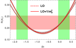
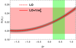
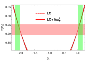
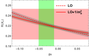
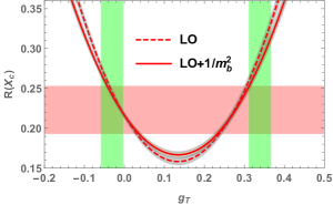
Figure 1: The ratio of decay rates $R(X_{c})$ (in $1S$ scheme) when one coupling at a time is present. The dashed red curves correspond to the case when the NP contribution is added at parton level while the solid red curves correspond to the case when power corrections are included in the NP contributions. Green bands are the constraints on the couplings due to $R(D^{(*)})_{exp}$ within $3\sigma$ and $B_{c}$ lifetime. The pink band is $R(X_{c})_{exp}$ within $1\sigma$.

In Fig. (1) we present the results (in the $1S$ scheme) for the observable $R(X_{c})$ when we turn on one NP coupling at a time. We consider two cases: the first case is when the NP contribution is considered only at parton level(dashed red curves), and the second case is when we add the subleading $1/m_{b}$ corrections to these NP contributions(solid red curves). The gray and brown bands correspond to the uncertainties of this observable when we vary the values of the parameters within their uncertainties. The green bands are the constraints on the couplings when we consider the measurements of $R(D^{(*)})$ within $3\sigma$. For the $g_{P}$ coupling, it is well known that the $B_{c}$ lifetime leads to a tight constraint Li:2016vvp ; Alonso:2016oyd ; Celis:2016azn . We use $\mathcal{B}(B_{c}\to\tau^{-}\bar{\nu}_{\tau})\leq 30\%$ as in Datta:2017aue , to include this constraint on the $g_{P}$ coupling which is included in the green band in the plot. The pink band, is the value of $R(X_{c})_{exp}$ within $1\sigma$.
In the parameter space of interest, adding the $1/m_{b}$ corrections to the NP contributions causes a change of $R(X_{c})$ that is numerically at percent level. This change is mostly noticeable in the $g_{S}$ and $g_{T}$ case where the maximum correction, in the parameter space that is favored by $R(D^{(*)})$, is $\approx 5\%$.

IV Conclusions

Recent measurements of $R(D^{(*)})$ show large deviations from ${\rm SM}$ predictions and this could be a signal of nonuniversal NP. The quark level transition in this observable is $b\to c\tau^{-}\bar{\nu}_{\tau}$ and we can probe this transition in other decay modes. In a recent work Kamali:2018fhr , we studied the inclusive $\bar{B}\to X_{c}\tau^{-}\bar{\nu}_{\tau}$ decay in view of the anomalies in the $R(D^{(*)})$ measurements. In this work we extended this study by including the effects of $1/m_{b}$ corrections in the NP Dirac structures. We presented the results of our calculations for the differential decay rate $\frac{d\Gamma}{dq^{2}}$ as well as the three-fold decay distribution and presented some numerical results of the effects of these power corrections on the observable $R(X_{c})$. By constraining the NP parameters by the existing $R(D^{(*)})$ measurements, we presented the favored parameter region by these measurements to illustrate if the power corrections in the NP part are important. We found that, in the parameter range of interest, these corrections are generically at percent level (except for the $g_{P}$ coupling which is smaller) and the maximum effect of these corrections is in the $g_{S}$ and $g_{T}$ part which is $\approx 5\%$.

Appendix A The three-fold differential distribution

In this appendix we present the three-fold differential rate in terms of invariant quantities. We write the distribution in the presence of all NP couplings in the form,

$$\frac{d^{3}\Gamma}{dx^{3}}= ~{}\frac{G_{F}^{2}|V_{cb}|^{2}}{8\pi^{3}}\Big{\{}|1+g_{L}|^{2}\frac{d^{3}\Gamma}{dx^{3}}\bigg{|}_{SM}+|g_{R}|^{2}\frac{d^{3}\Gamma}{dx^{3}}\bigg{|}_{R}+|g_{S}|^{2}\frac{d^{3}\Gamma}{dx^{3}}\bigg{|}_{S}+|g_{P}|^{2}\frac{d^{3}\Gamma}{dx^{3}}\bigg{|}_{P}+|g_{T}|^{2}\frac{d^{3}\Gamma}{dx^{3}}\bigg{|}_{T}$$

$$+Re((1+g_{L})g_{R}^{*})\frac{d^{3}\Gamma}{dx^{3}}\bigg{|}_{LR}+Re((1+g_{L}+g_{R})g_{S}^{*})\frac{d^{3}\Gamma}{dx^{3}}\big{|}_{SLR}$$

$$+Re((1+g_{L}-g_{R})g_{P}^{*})\frac{d^{3}\Gamma}{dx^{3}}\bigg{|}_{PLR}+Re((1+g_{L})g_{T}^{*})\frac{d^{3}\Gamma}{dx^{3}}\bigg{|}_{LT}+Re(g_{R}g_{T}^{*})\frac{d^{3}\Gamma}{dx^{3}}\bigg{|}_{RT}$$

$$+Re((g_{S}-g_{P})g_{T}^{*})\frac{d^{3}\Gamma}{dx^{3}}\bigg{|}_{SPT}\Big{\}},$$ (26)

where the three independent variables are usually taken to be $dx^{3}=dq^{2}dE_{\tau}dE_{\nu}$ or $dx^{3}=dq^{2}dE_{\tau}dq.v$, $v$ being the four velocity of the $B$ meson. Each contribution to the differential rate can be written as,

$$\frac{d^{3}\Gamma}{dx^{3}}\bigg{|}_{A}=\frac{1}{\Delta_{0}}\frac{d^{3}\Gamma}{dx^{3}}\bigg{|}_{A}^{(1)}+\frac{1}{\Delta_{0}^{2}}\frac{d^{3}\Gamma}{dx^{3}}\bigg{|}_{A}^{(2)}+\frac{1}{\Delta_{0}^{3}}\frac{d^{3}\Gamma}{dx^{3}}\bigg{|}_{A}^{(3)}.$$ (27)

Here we have defined $\Delta_{0}=p^{2}-m_{c}^{2}$ with $p=m_{b}v-q$. The contributions (27) to the decay distribution are given by the substitutions Manohar:1993qn ; Balk:1993sz ,

$$\frac{1}{\Delta_{0}}\quad \to\quad\delta(p^{2}-m_{c}^{2})$$

$$\frac{1}{\Delta_{0}^{2}}\quad \to\quad-\delta^{\prime}(p^{2}-m_{c}^{2})$$

$$\frac{1}{\Delta_{0}^{3}}\quad \to\quad\frac{1}{2}\delta^{\prime\prime}(p^{2}-m_{c}^{2}).$$ (28)

In the following we present various contributions to this distribution.
The ${\rm SM}$ contribution is given as,

$$\frac{d^{3}\Gamma}{dx^{3}}\bigg{|}_{SM}^{(1)}= ~{}\frac{4}{3m_{b}}\big{[}6m_{b}p.p_{\tau}p_{\nu}.v+(\lambda_{1}+3\lambda_{2})(2p_{\tau}.p_{\nu}-5p_{\tau}.vp_{\nu}.v)\big{]}$$ (29)

$$\frac{d^{3}\Gamma}{dx^{3}}\bigg{|}_{SM}^{(2)}= ~{}\frac{4}{3m_{b}}\big{[}2(\lambda_{1}+3\lambda_{2})(-2p.p_{\nu}+5p.vp_{\nu}.v)p.p_{\tau}+2m_{b}\lambda_{1}(2p.vp_{\tau}.v-5p.p_{\tau})p_{\nu}.v$$

$$+6m_{b}\lambda_{2}(p.vp_{\tau}.p_{\nu}-p.p_{\nu}p_{\tau}.v)\big{]}$$ (30)

$$\frac{d^{3}\Gamma}{dx^{3}}\bigg{|}_{SM}^{(3)}= ~{}\frac{32\lambda_{1}}{3}\big{[}p.p-(p.v)^{2}\big{]}p.p_{\tau}p_{\nu}.v~{}.$$ (31)

The $A=R$ contribution is derived from ${\rm SM}$ part by the substitutions $p_{\tau}\to p_{\nu}$ and $p_{\nu}\to p_{\tau}$,

$$\frac{d^{3}\Gamma}{dx^{3}}\bigg{|}_{R}^{(i)}=~{}\frac{d^{3}\Gamma}{dx^{3}}\bigg{|}_{SM}^{(i)}(p_{\tau}\leftrightarrow p_{\nu})\quad\quad i=1,2,3.$$ (32)

For $A=S$ we have,

$$\frac{d^{3}\Gamma}{dx^{3}}\bigg{|}_{S}^{(1)}= ~{}\frac{1}{2m_{b}^{2}}\big{[}2m_{b}^{2}(p.v+m_{c})+(m_{b}+m_{c})(\lambda_{1}+3\lambda_{2})\big{]}p_{\tau}.p_{\nu}$$ (33)

$$\frac{d^{3}\Gamma}{dx^{3}}\bigg{|}_{S}^{(2)}= ~{}-\frac{(\lambda_{1}+3\lambda_{2})}{3m_{b}}\big{[}3m_{b}(p.v+m_{c})-3m_{c}p.v+2p.p-5(p.v)^{2}\big{]}p_{\tau}.p_{\nu}$$ (34)

$$\frac{d^{3}\Gamma}{dx^{3}}\bigg{|}_{S}^{(3)}= ~{}\frac{4\lambda_{1}}{3}(p.v+m_{c})\big{[}p.p-(p.v)^{2}\big{]}p_{\tau}.p_{\nu}~{},$$ (35)

while the $A=P$ case can be derived from $A=S$ case by the substitution $m_{c}\to-m_{c}$,

$$\frac{d^{3}\Gamma}{dx^{3}}\bigg{|}_{P}^{(i)}= ~{}\frac{d^{3}\Gamma}{dx^{3}}\bigg{|}_{S}^{(i)}(m_{c}\to-m_{c})\quad\quad i=1,2,3.$$ (36)

For $A=T$ we find,

$$\frac{d^{3}\Gamma}{dx^{3}}\bigg{|}_{T}^{(1)}= ~{}\frac{16}{3m_{b}}\big{[}6m_{b}(2p.p_{\nu}p_{\tau}.v+2p.p_{\tau}p_{\nu}.v-p.vp_{\tau}.p_{\nu})+5(\lambda_{1}+3\lambda_{2})(p_{\tau}.p_{\nu}-4p_{\tau}.vp_{\nu}.v)\big{]}$$ (37)

$$\frac{d^{3}\Gamma}{dx^{3}}\bigg{|}_{T}^{(2)}= ~{}-\frac{32}{3m_{b}}\big{[}(\lambda_{1}+3\lambda_{2})(8p.p_{\tau}p.p_{\nu}-2p.pp_{\tau}.p_{\nu}+5(p.v)^{2}p_{\tau}.p_{\nu}-10p.p_{\nu}p.vp_{\tau}.v$$

$$-10p.p_{\tau}p.vp_{\nu}.v)+2m_{b}(5\lambda_{1}-3\lambda_{2})(p.p_{\nu}p_{\tau}.v+p.p_{\tau}p_{\nu}.v)$$

$$-3m_{b}(\lambda_{1}-\lambda_{2})p.vp_{\tau}.p_{\nu}-8m_{b}\lambda_{1}p.vp_{\tau}.vp_{\nu}.v\big{]}$$ (38)

$$\frac{d^{3}\Gamma}{dx^{3}}\bigg{|}_{T}^{(3)}= ~{}-\frac{128\lambda_{1}}{3}\big{[}p.p-(p.v)^{2}\big{]}\big{[}p.vp_{\tau}.p_{\nu}-2p.p_{\nu}p_{\tau}.v-2p.p_{\tau}p_{\nu}.v\big{]}$$ (39)

For $A=LR$,

$$\frac{d^{3}\Gamma}{dx^{3}}\bigg{|}_{LR}^{(1)}= ~{}-\frac{4m_{c}}{m_{b}^{2}}\big{(}2m_{b}^{2}+\lambda_{1}+3\lambda_{2}\big{)}p_{\tau}.p_{\nu}$$ (40)

$$\frac{d^{3}\Gamma}{dx^{3}}\bigg{|}_{LR}^{(2)}= ~{}\frac{8m_{c}}{m_{b}}\big{[}-(\lambda_{1}+3\lambda_{2})p.vp_{\tau}.p_{\nu}+m_{b}(\lambda_{1}+\lambda_{2})p_{\tau}.p_{\nu}-4m_{b}\lambda_{2}p_{\tau}.vp_{\nu}.v\big{]}$$ (41)

$$\frac{d^{3}\Gamma}{dx^{3}}\bigg{|}_{LR}^{(3)}= ~{}-\frac{32m_{c}\lambda_{1}}{3}\big{[}p.p-(p.v)^{2}\big{]}p_{\tau}.p_{\nu}$$ (42)

For $A=SLR$,

$$\frac{d^{3}\Gamma}{dx^{3}}\bigg{|}_{SLR}^{(1)}= ~{}\frac{m_{\tau}}{m_{b}^{2}}\big{[}2m_{b}^{2}(p.p_{\nu}+m_{c}p_{\nu}.v)+(\lambda_{1}+3\lambda_{2})(p.p_{\nu}-m_{b}p_{\nu}.v)\big{]}$$ (43)

$$\frac{d^{3}\Gamma}{dx^{3}}\bigg{|}_{SLR}^{(2)}= ~{}-\frac{2m_{\tau}}{3m_{b}}\big{[}(\lambda_{1}+3\lambda_{2})(-3p.p_{\nu}p.v+3m_{b}m_{c}p_{\nu}.v-5m_{c}p.vp_{\nu}.v+2m_{c}p.p_{\nu})$$

$$+m_{b}(5\lambda_{1}+3\lambda_{2})p.p_{\nu}-2m_{b}(\lambda_{1}-3\lambda_{2})p.vp_{\nu}.v\big{]}$$ (44)

$$\frac{d^{3}\Gamma}{dx^{3}}\bigg{|}_{SLR}^{(3)}= ~{}\frac{8m_{\tau}\lambda_{1}}{3}\big{[}p.p-(p.v)^{2}\big{]}\big{(}p.p_{\nu}+m_{c}p_{\nu}.v\big{)}$$ (45)

For $A=PLR$ we have,

$$\frac{d^{3}\Gamma}{dx^{3}}\bigg{|}_{PLR}^{(i)}= ~{}\frac{d^{3}\Gamma}{dx^{3}}\bigg{|}_{SLR}^{(i)}(m_{c}\to-m_{c})\quad\quad i=1,2,3.$$ (46)

For $A=LT$,

$$\frac{d^{3}\Gamma}{dx^{3}}\bigg{|}_{LT}^{(1)}= ~{}-48m_{\tau}m_{c}\big{(}p_{\nu}.v\big{)}$$ (47)

$$\frac{d^{3}\Gamma}{dx^{3}}\bigg{|}_{LT}^{(2)}= ~{}-\frac{16m_{\tau}m_{c}}{m_{b}}\big{[}(\lambda_{1}+3\lambda_{2})(-2p.p_{\nu}+5p.vp_{\nu}.v)-3m_{b}(\lambda_{1}-\lambda_{2})p_{\nu}.v\big{]}$$ (48)

$$\frac{d^{3}\Gamma}{dx^{3}}\bigg{|}_{LT}^{(3)}= ~{}-64m_{\tau}m_{c}\lambda_{1}\big{[}p.p-(p.v)^{2}\big{]}(p_{\nu}.v)$$ (49)

For $A=RT$,

$$\frac{d^{3}\Gamma}{dx^{3}}\bigg{|}_{RT}^{(1)}= ~{}\frac{24m_{\tau}}{m_{b}^{2}}\big{[}2m_{b}^{2}p.p_{\nu}+(\lambda_{1}+3\lambda_{2})(p.p_{\nu}-m_{b}p_{\nu}.v)\big{]}$$ (50)

$$\frac{d^{3}\Gamma}{dx^{3}}\bigg{|}_{RT}^{(2)}= ~{}-\frac{16m_{\tau}}{m_{b}}\big{[}-3(\lambda_{1}+3\lambda_{2})p.p_{\nu}p.v+m_{b}(5\lambda_{1}-\lambda_{2})p.p_{\nu}-2m_{b}(\lambda_{1}+\lambda_{2})p.vp_{\nu}.v\big{]}$$ (51)

$$\frac{d^{3}\Gamma}{dx^{3}}\bigg{|}_{RT}^{(3)}= ~{}64m_{\tau}\lambda_{1}\big{[}p.p-(p.v)^{2}\big{]}\big{(}p.p_{\nu}\big{)}$$ (52)

For $A=SPT$,

$$\frac{d^{3}\Gamma}{dx^{3}}\bigg{|}_{SPT}^{(1)}= ~{}8\big{(}p.p_{\nu}p_{\tau}.v-p.p_{\tau}p_{\nu}.v\big{)}$$ (53)

$$\frac{d^{3}\Gamma}{dx^{3}}\bigg{|}_{SPT}^{(2)}= ~{}\frac{8}{3m_{b}}\big{[}5(\lambda_{1}+3\lambda_{2})p.v-m_{b}(5\lambda_{1}+3\lambda_{2})\big{]}\big{(}p.p_{\nu}p_{\tau}.v-p.p_{\tau}p_{\nu}.v\big{)}$$ (54)

$$\frac{d^{3}\Gamma}{dx^{3}}\bigg{|}_{SPT}^{(3)}= ~{}\frac{32\lambda_{1}}{3}\big{[}p.p-(p.v)^{2}\big{]}\big{(}p.p_{\nu}p_{\tau}.v-p.p_{\tau}p_{\nu}.v\big{)}$$ (55)

References

- (1) BaBar Collaboration, J. P. Lees et al., “Measurement of an Excess of Decays and Implications for Charged Higgs Bosons,” Phys. Rev. D88 no. 7, (2013) 072012, arXiv:1303.0571 [hep-ex].
- (2) BaBar Collaboration, J. P. Lees et al., “Evidence for an excess of decays,” Phys. Rev. Lett. 109 (2012) 101802, arXiv:1205.5442 [hep-ex].
- (3) Belle Collaboration, M. Huschle et al., “Measurement of the branching ratio of relative to decays with hadronic tagging at Belle,” Phys. Rev. D92 no. 7, (2015) 072014, arXiv:1507.03233 [hep-ex].
- (4) Belle Collaboration, A. Abdesselam et al., “Measurement of the branching ratio of relative to decays with a semileptonic tagging method,” in Proceedings, 51st Rencontres de Moriond on Electroweak Interactions and Unified Theories: La Thuile, Italy, March 12-19, 2016. 2016. arXiv:1603.06711 [hep-ex].
- (5) Belle Collaboration, Y. Sato et al., “Measurement of the branching ratio of relative to decays with a semileptonic tagging method,” Phys. Rev. D94 no. 7, (2016) 072007, arXiv:1607.07923 [hep-ex].
- (6) Belle Collaboration, S. Hirose et al., “Measurement of the lepton polarization and in the decay ,” Phys. Rev. Lett. 118 no. 21, (2017) 211801, arXiv:1612.00529 [hep-ex].
- (7) LHCb Collaboration, R. Aaij et al., “Measurement of the ratio of branching fractions ,” Phys. Rev. Lett. 115 no. 11, (2015) 111803, arXiv:1506.08614 [hep-ex]. [Erratum: Phys. Rev. Lett.115,no.15,159901(2015)].
- (8) A. Celis, M. Jung, X.-Q. Li, and A. Pich, “Sensitivity to charged scalars in and decays,” JHEP 01 (2013) 054, arXiv:1210.8443 [hep-ph].
- (9) M. Duraisamy and A. Datta, “The Full Angular Distribution and CP violating Triple Products,” JHEP 09 (2013) 059, arXiv:1302.7031 [hep-ph].
- (10) A. Crivellin, A. Kokulu, and C. Greub, “Flavor-phenomenology of two-Higgs-doublet models with generic Yukawa structure,” Phys. Rev. D87 no. 9, (2013) 094031, arXiv:1303.5877 [hep-ph].
- (11) I. Doršner, S. Fajfer, N. Košnik, and I. Nišandžić, “Minimally flavored colored scalar in and the mass matrices constraints,” JHEP 11 (2013) 084, arXiv:1306.6493 [hep-ph].
- (12) M. Freytsis, Z. Ligeti, and J. T. Ruderman, “Flavor models for ,” Phys. Rev. D92 no. 5, (2015) 054018, arXiv:1506.08896 [hep-ph].
- (13) N. G. Deshpande and X.-G. He, “Consequences of R-parity violating interactions for anomalies in and ,” Eur. Phys. J. C77 no. 2, (2017) 134, arXiv:1608.04817 [hep-ph].
- (14) S. Bhattacharya, S. Nandi, and S. Kumar Patra, “ Decays: A Catalogue to Compare, Constrain, and Correlate New Physics Effects,” arXiv:1805.08222 [hep-ph].
- (15) A. Datta, M. Duraisamy, and D. Ghosh, “Diagnosing New Physics in decays in the light of the recent BaBar result,” Phys. Rev. D86 (2012) 034027, arXiv:1206.3760 [hep-ph].
- (16) M. Duraisamy, P. Sharma, and A. Datta, “Azimuthal angular distribution with tensor operators,” Phys. Rev. D90 no. 7, (2014) 074013, arXiv:1405.3719 [hep-ph].
- (17) B. Bhattacharya, A. Datta, D. London, and S. Shivashankara, “Simultaneous Explanation of the and Puzzles,” Phys. Lett. B742 (2015) 370–374, arXiv:1412.7164 [hep-ph].
- (18) J. A. Bailey et al., “Refining new-physics searches in decay with lattice QCD,” Phys. Rev. Lett. 109 (2012) 071802, arXiv:1206.4992 [hep-ph].
- (19) MILC Collaboration, J. A. Bailey et al., “ form factors at nonzero recoil and —Vcb— from 2+1-flavor lattice QCD,” Phys. Rev. D92 no. 3, (2015) 034506, arXiv:1503.07237 [hep-lat].
- (20) HPQCD Collaboration, H. Na, C. M. Bouchard, G. P. Lepage, C. Monahan, and J. Shigemitsu, “ form factors at nonzero recoil and extraction of ,” Phys. Rev. D92 no. 5, (2015) 054510, arXiv:1505.03925 [hep-lat]. [Erratum: Phys. Rev.D93,no.11,119906(2016)].
- (21) D. Bigi and P. Gambino, “Revisiting ,” Phys. Rev. D94 no. 9, (2016) 094008, arXiv:1606.08030 [hep-ph].
- (22) D. Bigi, P. Gambino, and S. Schacht, “, , and the Heavy Quark Symmetry relations between form factors,” JHEP 11 (2017) 061, arXiv:1707.09509 [hep-ph].
- (23) F. U. Bernlochner, Z. Ligeti, M. Papucci, and D. J. Robinson, “Combined analysis of semileptonic decays to and : , , and new physics,” Phys. Rev. D95 no. 11, (2017) 115008, arXiv:1703.05330 [hep-ph]. [Erratum: Phys. Rev.D97,no.5,059902(2018)].
- (24) S. Jaiswal, S. Nandi, and S. K. Patra, “Extraction of from and the Standard Model predictions of ,” JHEP 12 (2017) 060, arXiv:1707.09977 [hep-ph].
- (25) Heavy Flavor Averaging Group Collaboration, Y. Amhis et al., “Averages of -hadron, -hadron, and -lepton properties as of summer 2016,” Eur. Phys. J. C77 (2017) 895, arXiv:1612.07233 [hep-ex]. updated results and plots available at https://hflav.web.cern.ch.
- (26) S. Kamali, A. Rashed, and A. Datta, “New physics in inclusive decay in light of measurements,” Phys. Rev. D97 no. 9, (2018) 095034, arXiv:1801.08259 [hep-ph].
- (27) Y. Grossman and Z. Ligeti, “The Inclusive decay in two Higgs doublet models,” Phys. Lett. B332 (1994) 373–380, arXiv:hep-ph/9403376 [hep-ph].
- (28) P. Colangelo and F. De Fazio, “Tension in the inclusive versus exclusive determinations of : a possible role of new physics,” Phys. Rev. D95 no. 1, (2017) 011701, arXiv:1611.07387 [hep-ph].
- (29) A. V. Manohar and M. B. Wise, “Inclusive semileptonic B and polarized decays from QCD,” Phys. Rev. D49 (1994) 1310–1329, arXiv:hep-ph/9308246 [hep-ph].
- (30) S. Balk, J. G. Korner, D. Pirjol, and K. Schilcher, “Inclusive semileptonic B decays in QCD including lepton mass effects,” Z. Phys. C64 (1994) 37–44, arXiv:hep-ph/9312220 [hep-ph].
- (31) A. F. Falk, M. E. Luke, and M. J. Savage, “Nonperturbative contributions to the inclusive rare decays and ,” Phys. Rev. D49 (1994) 3367–3378, arXiv:hep-ph/9308288 [hep-ph].
- (32) L. Koyrakh, “Nonperturbative corrections to the heavy lepton energy distribution in the inclusive decays ,” Phys. Rev. D49 (1994) 3379–3384, arXiv:hep-ph/9311215 [hep-ph].
- (33) A. F. Falk, Z. Ligeti, M. Neubert, and Y. Nir, “Heavy quark expansion for the inclusive decay ,” Phys. Lett. B326 (1994) 145–153, arXiv:hep-ph/9401226 [hep-ph].
- (34) B. Blok, L. Koyrakh, M. A. Shifman, and A. I. Vainshtein, “Differential distributions in semileptonic decays of the heavy flavors in QCD,” Phys. Rev. D49 (1994) 3356, arXiv:hep-ph/9307247 [hep-ph]. [Erratum: Phys. Rev.D50,3572(1994)].
- (35) Z. Ligeti and F. J. Tackmann, “Precise predictions for decay distributions,” Phys. Rev. D90 no. 3, (2014) 034021, arXiv:1406.7013 [hep-ph].
- (36) B. M. Dassinger, T. Mannel, and S. Turczyk, “Inclusive semi-leptonic B decays to order ,” JHEP 03 (2007) 087, arXiv:hep-ph/0611168 [hep-ph].
- (37) A. H. Hoang, Z. Ligeti, and A. V. Manohar, “B decay and the Upsilon mass,” Phys. Rev. Lett. 82 (1999) 277–280, arXiv:hep-ph/9809423 [hep-ph].
- (38) A. H. Hoang, Z. Ligeti, and A. V. Manohar, “B decays in the upsilon expansion,” Phys. Rev. D59 (1999) 074017, arXiv:hep-ph/9811239 [hep-ph].
- (39) D. Benson, I. I. Bigi, T. Mannel, and N. Uraltsev, “Imprecated, yet impeccable: On the theoretical evaluation of Gamma(B —¿ X(c) l nu),” Nucl. Phys. B665 (2003) 367–401, arXiv:hep-ph/0302262 [hep-ph].
- (40) P. Gambino and N. Uraltsev, “Moments of semileptonic B decay distributions in the 1/m(b) expansion,” Eur. Phys. J. C34 (2004) 181–189, arXiv:hep-ph/0401063 [hep-ph].
- (41) P. Gambino, “B semileptonic moments at NNLO,” JHEP 09 (2011) 055, arXiv:1107.3100 [hep-ph].
- (42) A. Alberti, P. Gambino, K. J. Healey, and S. Nandi, “Precision Determination of the Cabibbo-Kobayashi-Maskawa Element ,” Phys. Rev. Lett. 114 no. 6, (2015) 061802, arXiv:1411.6560 [hep-ph].
- (43) C. W. Bauer, Z. Ligeti, M. Luke, and A. V. Manohar, “B decay shape variables and the precision determination of —V(cb)— and m(b),” Phys. Rev. D67 (2003) 054012, arXiv:hep-ph/0210027 [hep-ph].
- (44) C. W. Bauer, Z. Ligeti, M. Luke, A. V. Manohar, and M. Trott, “Global analysis of inclusive B decays,” Phys. Rev. D70 (2004) 094017, arXiv:hep-ph/0408002 [hep-ph].
- (45) T. Mannel, A. V. Rusov, and F. Shahriaran, “Inclusive semitauonic decays to order ,” Nucl. Phys. B921 (2017) 211–224, arXiv:1702.01089 [hep-ph].
- (46) V. Aquila, P. Gambino, G. Ridolfi, and N. Uraltsev, “Perturbative corrections to semileptonic b decay distributions,” Nucl. Phys. B719 (2005) 77–102, arXiv:hep-ph/0503083 [hep-ph].
- (47) M. Jezabek and L. Motyka, “Tau lepton distributions in semileptonic B decays,” Nucl. Phys. B501 (1997) 207–223, arXiv:hep-ph/9701358 [hep-ph].
- (48) S. Biswas and K. Melnikov, “Second order QCD corrections to inclusive semileptonic decays with massless and massive lepton,” JHEP 02 (2010) 089, arXiv:0911.4142 [hep-ph].
- (49) ALEPH Collaboration, R. Barate et al., “Measurements of and and upper limits on and ,” Eur. Phys. J. C19 (2001) 213–227, arXiv:hep-ex/0010022 [hep-ex].
- (50) LHCb Collaboration, R. Aaij et al., “Determination of the quark coupling strength using baryonic decays,” Nature Phys. 11 (2015) 743–747, arXiv:1504.01568 [hep-ex].
- (51) A. Celis, M. Jung, X.-Q. Li, and A. Pich, “Scalar contributions to transitions,” Phys. Lett. B771 (2017) 168–179, arXiv:1612.07757 [hep-ph].
- (52) X.-Q. Li, Y.-D. Yang, and X. Zhang, “Revisiting the one leptoquark solution to the R(D(∗)) anomalies and its phenomenological implications,” JHEP 08 (2016) 054, arXiv:1605.09308 [hep-ph].
- (53) R. Alonso, B. Grinstein, and J. Martin Camalich, “Lifetime of Constrains Explanations for Anomalies in ,” Phys. Rev. Lett. 118 no. 8, (2017) 081802, arXiv:1611.06676 [hep-ph].
- (54) A. Datta, S. Kamali, S. Meinel, and A. Rashed, “Phenomenology of using lattice QCD calculations,” JHEP 08 (2017) 131, arXiv:1702.02243 [hep-ph].