Deep Learning with Inaccurate Training Data for Image Restoration

Abstract

In many applications of deep learning, particularly those in image restoration, it is either very difficult, prohibitively expensive, or outright impossible to obtain paired training data precisely as in the real world. In such cases, one is forced to use synthesized paired data to train the deep convolutional neural network (DCNN). However, due to the unavoidable generalization error in statistical learning, the synthetically trained DCNN often performs poorly on real world data. To overcome this problem, we propose a new general training method that can compensate for, to a large extent, the generalization errors of synthetically trained DCNNs.

1 Introduction

Over the past few years deep learning has become a widely advocated approach for image restoration. A large number of research papers have been published on the use of deep convolutional neural networks (DCNN) for image super-resolution, denoising, deblurring, demosaicking, descreening, etc. All these authors reported great improvements of the restoration results by the DCNN methods over traditional image processing methods. However, as demonstrated by this work, there is still a technical hurdle to be cleared, before one can firmly establish the superiority of data-driven deep learning approach to the traditional model-based inverse problem framework for image restoration.

(a) Bicubic

(b) EDSR

(c) Ground truth

(d) Bicubic

(e) EDSR

(f) EDSR+

Figure 1: Sample $\times 4$ super-resolution results of the original EDSR model and our refined version, EDSR+. Although EDSR performs well for synthetic low-resolution input image (first row), it is ineffective for real image (second row) in comparison with EDSR+

In the vast majority of the published studies on deep learning image restoration, the pairs of high-quality and degraded images for training the neural networks are generated synthetically using a simplistic degradation model. For example, in all deep learning super-resolution papers, the low-resolution images are generated from their full resolution counterparts via some downsampling kernel like bicubic. But the actual physical formations of such images are far more complex and compounded, involving various factors such as the camera point spread function (PSF), pixel sensors crosstalk, demosaicking, compression, camera/object motion, etc. The discrepancy between the downsampling operator and the true signal degradation function is more than enough to derail these learning methods. As exemplified in Figure 1, although the existing deep learning super-resolution methods perform very well on artificially generated low-resolution images, they cannot super-resolve real-world images nearly at the same quality. Unfortunately, many outstanding image restoration results reported in the literature, which are obtained with perfect match of the data for training and inference in statistics, are somewhat misleading and irreproducible on real images.

A more sophisticated data synthesizer is certainly warranted to realize the full potential of a deep learning method on real data. But in many applications of image restoration, it is very difficult, if not impossible, to simulate the complex compound effects of multiple degradation causes, some of which may be stochastic, to the desired precision. To further demonstrate this difficulty in the paper, we also study the problem of demoiré, the task of removing the interference patterns in a camera-captured screen image, in addition to super-resolution. In this case, given an original image, its degraded version after being displayed on screen and then captured by camera may be synthesized approximately for training using a very complex image formation model, but the accuracy of the synthesis is still insufficient due to intricate interplays of lens distortion, defocus blur, screen glass glare, etc.

Very recently, the issue of statistically mismatched training data in DCNN image denoising methods was getting brought up and discussed [13, 1, 2, 15]. After pointing out the pitfalls of using simple Gaussian noise model to create noisy and clean image pairs to train DCNNs, these authors proposed to alleviate the problem by generating more realistic paired training images, either using data acquired in extensive experiments with an assortment of cameras operating in different ISO settings, or using generative adversarial network (GAN) to combine clean images with noise extracted from real noisy images. However, the paired training data generated by the above improved techniques are still synthesized after all; inevitably, they deviate from those in the real world situations.

As outlined above, the most likely scenario for a deep learning image restoration system is that, even with the best degradation model $M$ on hand, artificially degraded image $Y_{s}=M(X)$ from clean image $X$ still differs greatly from real degraded image $Y$. Thus, although the synthetic-real image pairs $(Y_{s};X)$ can be used to train a generative DCNN $G_{0}$ directly as in current practice, the resulting $G_{0}$ is often ineffective for real images.

In our design, the algorithm development does not end with $G_{0}$. Instead, the synthetically trained restoration DCNN $G_{0}$ is used to produce so-called surrogate ground truth images $X_{s}$ to pair up with real degraded input images $Y$, when the real ground truth images $X$ for $Y$ cannot be obtained. In other words, we feed $Y$ into the DCNN $G_{0}$ to generate the corresponding restored images $X_{s}=G_{0}(Y)$. The real degraded images $Y$ and their surrogate ground truth images $X_{s}$, the latter being approximations of $X$, provide the paired data $(Y;X_{s})$ to refine the restoration network $G_{0}$ through supervised learning.

We would like to stress a vital difference between the existing methods and our method. Previous authors used real pristine images $X$ but paired them with synthetic degraded images in the training of restoration DCNNs. In contrast, we stick to real degraded images $Y$ and pair them with synthetic ground truth images $X_{s}$. We argue, also as demonstrate by empirical results, that the latter approach is the correct one.

When practical limitations prevent the deep learning algorithm designers from having the ideal paired training data $(Y;X)$ that are exact as the physical reality, they have two options as to choosing paired training data: $(Y_{s};X)$ or $(Y;X_{s})$. There is an obvious paradox in using the paired synthetic-real data $(Y_{s};X)$ to train the restoration DCNN. At the time of inference, the DCNN needs to estimate the latent image $X$ from the real degraded image $Y$, not from the synthetic one $Y_{s}$ as in the training. Moreover, it is operationally very difficult, if not impossible, in the DCNN design stage to account for the imprecisions in the synthetic input data $Y_{s}$.

On the other hand, by taking the second option, we train the restoration DCNN to work with the real input degraded images $Y$. Although in the training stage, we have to use surrogate ground truth images $X_{s}$ at the output end of the network, we can easily include suitable penalty terms in the objective function to remove or alleviate the effects of differences between $X_{s}$ and $X$. An immediate idea is to use the GAN technique to augment the signal level fidelity of the paired data by the statistics of unpaired clean images.

In addition to the above highlighted contribution, the proposed new training method is a general one; it can be applied to improve any existing DCNNs for image restoration, regardless the specific application problems addressed.

2 Related Work

The problem of statistical differences between synthetic and real data has long been overlooked in the literature of learning based image restoration. Not until recently have there been a few attempts to alleviate the problem in some specific applications, such as denoising and super-resolution. Most of these studies focus on improving the truthfulness of their training data synthesizers. For instance, to generate artificial noise for multi-image denoising, [11] first converts images to linear color space with real data calibrated invert gamma correction and then generates noise with distribution estimated from real images. For single image denoising, [6] employs a sophisticated noise synthesizer that takes multiple factors into consideration, such as signal-dependent noise and camera processing pipeline. In [2], the authors proposed a GAN-based neural network to generate realistic camera noise. The network is trained with high-quality images superimposed with noise patterns extracted from smooth regions of real noisy images, assuming that the high frequency components of these smooth regions only come from sensor noise and noise is independent to signal. These assumptions however are impractical and restrictive, making it difficult to extend the idea for other image restoration problems.

The problem of inaccurate degradation model is also recognized by the authors of [14] in their study of data-driven super-resolution. To alleviate the problem, they proposed a relatively shallow neural network, called ZSSR, which is trained only with patches aggregated from the input image. However, ZSSR still relies on bicubic downsampling to synthesize the corresponding low-resolution patches; the problem of the unrealistic downsampler is left unaddressed.

Another possible option is to give up explicit degradation model completely and use unpaired training instead. CycleGAN provides a mechanism to construct a bi-directional mapping between two types of images without paired samples [18, 16]. However, the learning of the degradation process can be extremely challenging without precisely aligned data let alone restoration. Thus, it is difficult to achieve highly accurate results using this approach.

Due to the complexity of image formation, it is extremely difficult to design a good data synthesizer in many image restoration applications. Even the seemingly minor details of a synthetic process, such as whether the noise values are rounded to integers, can have a significant impact on the performance of a deep learning technique [3]. Thus, instead of using data synthesis, many studies try to use extra images captured in non-ideal conditions as the input. For example, by using different camera exposure settings, one can obtain a series of images of the same scene with varied noise levels and then use the underexposed ones as the noisy input [13]. To train a deblurring DCNN, one can average all the frames of a high frame-rate video clip as the blurry input and pick one of the frames as the sharp ground truth image [12]. While employing extra images mitigates the problem of inaccurate synthesizer, it suffers from several serious drawbacks. First, due to the nature of using multiple images, the imaged subject must stay perfectly still, and complex image processing operators, such as lens correction, spatial alignment, intensity matching are required to couple the high-quality and degraded image. Second, as it is often prohibitively expensive to build a sufficiently large data set by taking images one by one, a network can overfit the available data and become sensitive to particular camera brands, exposure settings and captured scenes [15].

3 Two-Stage Training

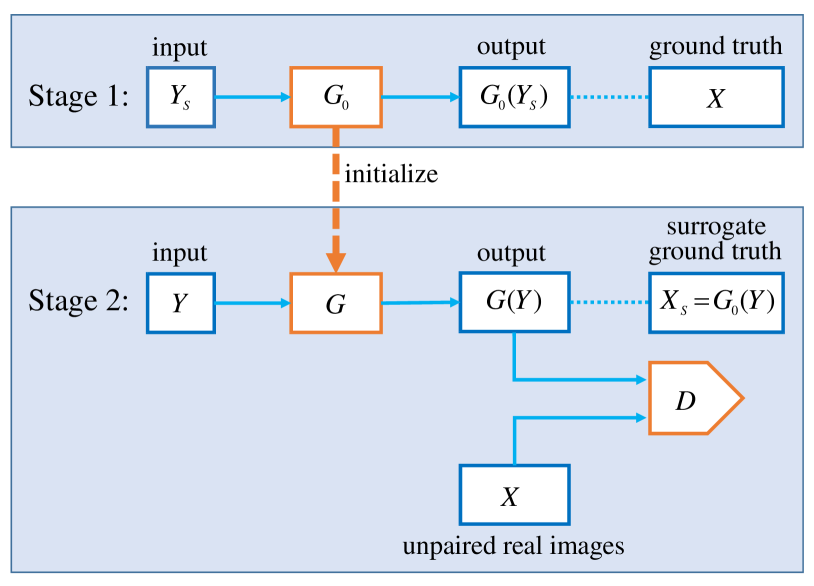
Figure 2: The proposed two-stage learning approach.

Due to the lack of paired real data, most existing deep learning image restoration techniques train their DCNNs $G_{0}$ with artificially degraded images $Y_{s}$ paired with the corresponding high-quality ground truth images $X$. However, as we discussed previously, this mainstream approach is fundamentally flawed: a DCNN, which has never “seen” any real degraded images in training, performs unsatisfactorily for real images. In this section, we introduce an alternative training approach, which circumvents the aforementioned problem by using real degraded images $Y$ and surrogate ground truth images $X_{s}$ as the training data.

In most applications, collecting a large number of real degraded images $Y$ that are governed by the same distribution as the real input is not difficult, but it is a challenging task to find an accurate estimate $X_{s}$ of the corresponding latent ground truth image $X$. After all, that is exactly the restoration problem that we want to solve. However, even if we have to resort to inaccurate surrogate ground truth images $X_{s}$ in the training of a DCNN $G$, there are still various ways to rectify the final output $G(Y)$. In other words, with fitting image priors and properly designed penalty terms, imperfect the surrogate ground truth images might not severely affect the training of $G$ for real degraded input images. Thus, we can simply train a DCNN $G_{0}$ as the synthesizer using artificially degraded images $Y_{s}$ and real ground truth $X$, and then generate the surrogate ground truth images $X_{s}$ by feeding $G_{0}$ with real degrades images $Y$, i.e., let $X_{s}=G_{0}(Y)$.

Based on the above idea, we design a two-stage training approach, as sketched in Figure 2. In the first stage, the DCNN $G_{0}$ is trained using the conventional approach with synthetic input $Y_{s}$ and real ground truth $X$. Then in the second stage, the network is retrained as $G$ using real degraded image $Y$ and surrogate ground truth $G_{0}(Y)$ generated by the first stage network $G_{0}$. Due to the similarities of their training data, the second training stage can be significantly expedited by initializing $G$ using the weights of $G_{0}$. While the synthetically trained $G_{0}$ can produce a rough estimate $X_{s}$ of the latent ground truth for any given real degraded image $Y$, the output $G_{0}(Y)$ is often plagued with artifacts. To prevent these objectionable artifacts from being picked up by $G$, we include additional penalty terms, such as GAN, in the objective function of the second stage.

The proposed training approach is a general one, applicable to any existing image restoration DCNN techniques regardless of their network architectures or objective functions. For instance, many restoration techniques optimize pixel-wise loss function, such as mean squared error (MSE), in the training of their networks, as follows,

$$L_{2} =\frac{1}{WH}\|G_{0}(Y_{s})-X\|_{2}^{2},$$ (1)

where the $W$ and $H$ are the width and height of the network output, respectively. With our two-stage training approach, we can use these objective functions unaltered in the first training stage. Since the network architecture also requires no modification, the trained model from the original authors, if available, can be used as $G_{0}$ directly without retraining the network. In the second stage, the training set is consist of real-synthetic pairs $(Y;X_{s})$ instead of synthetic-real pairs $(Y_{s};X)$. Correspondingly, the example MSE loss function can be written as,

$$L_{2}\!=\!\frac{1}{W\!H}\|G(Y)\!-\!X_{s}\|_{2}^{2}\!=\!\frac{1}{W\!H}\|G(Y)\!-\!G_{0}(Y)\|_{2}^{2}.$$ (2)

In this second stage, the fidelity terms in objective function penalizes the differences between the output $G(Y)$ and the surrogate ground truth $X_{s}$, pushing $G$ to produce similar results as network $G_{0}$. As network $G_{0}$ is essentially a trained inverse of the degradation synthesizer function $M$, these fidelity terms implicitly regulates $G$ as an inverse of $M$ as well.

In addition to the fidelity terms, we also need to ensure the output $G(Y)$ is similar to real ground truth images statistically. Without the matched ground truth $X$ to $Y$, a possible solution to the problem is to use unpaired learning techniques. In the proposed training approach, we integrate the GAN technique in the second stage [4]. In GAN, a discriminative network $D$ is jointly trained with the generative network $G$ for discriminating the output images $G(Y)$ against a set of unpaired clean images $X$. This process guides $G$ to return images that are statistically similar to artifact-free ground truth images without using paired training data.

Following the idea of GAN, we set the discriminative network $D$ to solve the following minimax problem:

$$\min_{G}\max_{D}( \mathbb{E}_{X}\left[\log D(X)\right]$$

$$+\mathbb{E}_{Y}\left[\log(1-D(G(Y)))\right]).$$ (3)

This introduces an adversarial term in the loss function of the generator network $G$:

$$L_{A}=-\log D(G(Y)).$$ (4)

In competition against generator network $G$, the loss function for training discriminative network $D$ is the binary cross entropy:

$$L_{D}=-\left[\log(D(X))+\log(1-D(G(Y)))\right].$$ (5)

Minimizing $L_{A}$ drives network $G$ to produce images that network $D$ cannot distinguish from original artifact-free images. Accompanying the evolution of $G$, minimizing $L_{D}$ increases the discrimination power of network $D$.

Combining the MSE loss $L_{2}$ and adversarial loss $L_{A}$, we arrive at the final formulation of the loss function for optimizing $G$ in the second training stage,

$$L_{G}=L_{2}+\lambda L_{A},$$ (6)

where Lagrange multiplier $\lambda$ is user given weight balancing the two terms.

In the next two sections, we apply the proposed two-stage training approach in two very different image restoration problems to showcase the efficacy and generality of the idea.

4 Experiment on Face Super-Resolution

Super-resolution is one of the most intensively researched image restoration problems. In the last few years, DCNN-based Super-resolution techniques have demonstrated its great potential and significantly advanced the state of the art. However, almost all of these techniques still rely on unrealistic degradation models, such as bicubic downsampling, to synthesize training data, causing generalization problems in real-world applications. In this section, we select two popular super-resolution techniques, SRResNet [8] and EDSR [9], and try to improve their performance on real low-resolution images with the proposed two-stage training approach. We also test ZSSR [14], a super-resolution technique designed specifically for real images, and SRGAN [8], a GAN-based super-resolution technique, as references.

4.1 Preparation of Training Data

There are plenty of human face data sets available to researchers, but images in most of these sets were captured in controlled laboratory environment and none of them provides the required real low-resolution images for this research. Thus, we have to build our own face image data sets. The face images in our data set are cropped directly from video clips; no other image processing operators is used. The imaged persons are ethnically Asian, in various age groups and with different facial expressions and poses. The extracted face images are in two different resolutions: high-resolution ($120\times 120$) and low-resolution ($30\times 30$). The high-resolution images are used as the real ground truth images $X$, and the low-resolution images are used as the real degraded images $Y$. The artificially degraded images $Y_{s}$ are scaled down from $X$ using $\times 4$ bicubic downsampling.

4.2 Training Details

Of the 60,000 high-resolution face images in our data set, 40,000 are used for training SRResNet, EDSR and SRGAN; 10,000 images are for validation; and another 10,000 are for testing. The improved versions of SRResNet and EDSR by our training approach are called SRResNet+ and EDSR+ respectively. In the second training stage, SRResNet+ and EDSR+ use 10,000 real low-resolution images as input and 10,000 high-resolution images as unpaired real images for GAN. Moreover, SRGAN is also trained with the same unpaired real images for its GAN.

All the tested techniques, SRResNet, EDSR, ZSSR and SRGAN, are trained using the recommended settings by their authors. The loss function of SRResNet+ and EDSR+ in the second training stage is set as,

$$L_{G}=L_{2}+10^{-3}\times L_{A},$$ (7)

and the learning rate and batch size are set as $10^{-4}$ and 32, respectively. The second training stage takes $10^{4}$ update iterations, which are $1/10$ of the amount used by the first stage. Thus, the required time for the second training stage is roughly $1/10$ of the first. For GAN training, we set $k=1$ and update $G$ and the discriminator $D$ alternatively.

4.3 Experimental Results

(a) Bicubic

(b) SRResNet

(c) EDSR

(d) Ground truth

Figure 3: Results of $\times 4$ super-resolution for synthetic low-resolution images.

As shown in Figure  3, both SRResNet and EDSR perform well on our synthetic data set, scoring average peak signal-to-noise ratio (PSNR) 30.98 dB and 31.10 dB, respectively. Their output images are very similar to the ground truth images visually.

(a) Bicubic

(b) ZSSR

(c) SRResNet

(d) SRGAN

(e) EDSR

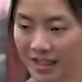
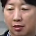
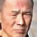
(f) SRResNet+

(g) EDSR+

Figure 4: Results of $\times 4$ super-resolution for real low-resolution images.

However, as shown in Figure 4, neither SRResNet nor EDSR can super-resolve real low-resolution images to the same quality level as the synthetic one. Even SRGAN, the GAN optimized version of SRResNet, is incapable of improving the performance for real images. Although to a human viewer, there are hardly any differences between the real and synthetic low-resolution images, the super-resolution results by the conventionally trained techniques are substantially different. In comparison, SRResNet+ and EDSR+, which are trained using the proposed approach, have no difficulty in real image super-resolution. Their results recover lots of details and look similar to the results of SRResNet and EDSR for synthetic images. Please note that the improved techniques share the exact same network architectures as the original versions; only weights are adjusted for dealing with real images.

We also test ZSSR, which only needs the low-resolution input image for training and testing. To make a fair comparison, we use the whole frame, instead of only a face image, as the input. However, its results are still inferior than the results of the other tested techniques.

5 Experiment on Demoiréing

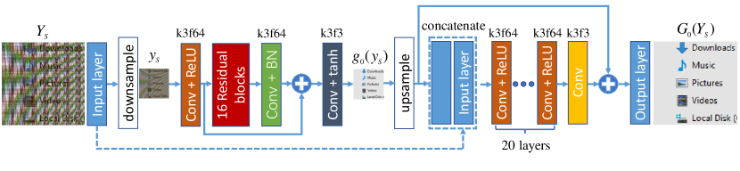
Figure 5: The architecture of the proposed DM-Net. The kernel size $k$ and the number of feature maps $f$ are marked above each convolutional layer.

In this section, we demonstrate the proposed two-stage training technique for another image restoration problem: demoiréing for camera-captured screen images. Taking photos of optoelectronic displays is a direct and spontaneous way of transferring data and keeping records, which is widely practiced. However, due to the analog signal interference between the pixel grids of the display screen and camera sensor array, objectionable moiré (alias) patterns appear in captured screen images. As the moiré patterns are structured, highly variant and correlated with signal, they are difficult to be completely removed without affecting the underneath latent image. Despite the commonness and annoyance of the problem, little work has been done on the reduction of moiré artifacts in camera-captured screen images.

To solve this challenging problem, we purposefully designed a multi-scale DCNN, called DM-Net. As shown in Figure 5, an input moiré image is first downsampled by a scale factor of 4 in DM-Net and demoiréd by 16 deep residual blocks as in [5]. The result is then upsampled to the original resolution and further cleaned up by 20 more convolutional layers. We also experimented with two excellent general purpose image restoration networks, DnCNN [17] and RED-Net [10], and retrained them for the demoiréing task using synthetic moiré images. While these techniques can produce more-or-less acceptable results for synthetic moiré images, their performances deteriorate significantly when dealing with real images.

We tried to solve the problem for real images using CycleGAN [18, 16]. It is however problematic for this task. As CycleGAN maps image $x$ to its clean version $G_{C}(x)$ then back ($F(G_{C}(x))=x$), it requires a one-to-one correspondence between the two images. But this does not hold for moiré images; there can be multiple images of the same content but vastly different moiré patterns. Moreover, without using paired data, the inverse mapping $F$ is unable to learn the degradation process precisely. As a result, the outputs of $F$ never become as realistic as those of our carefully designed moiré pattern synthesizer. Therefore, CycleGAN does not make an improvement over the existing results.

In the section, we demonstrate the efficacy of the proposed two-stage training approach for real image demoiríng.

5.1 Preparation of Training Data

Ideally, the training process should only use real photographs of a screen and the corresponding original digital images displayed on it. While obtaining such a pair of images is easy, perfectly aligning them spatially, a necessary condition for preventing mismatched edges being misidentified as moiré patterns, is difficult to achieve. As many common imaging problems in real photos, such as lens distortion and non-uniform camera shake, adversely affect the accuracy of image alignment, it is challenging to build a sufficiently large and high quality training set using real photos.

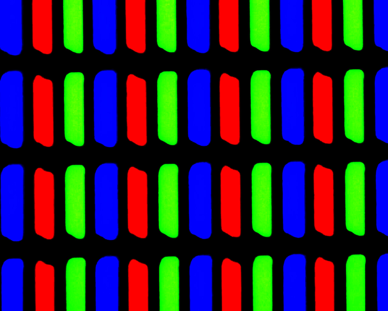
(a) LCD subpixel structure

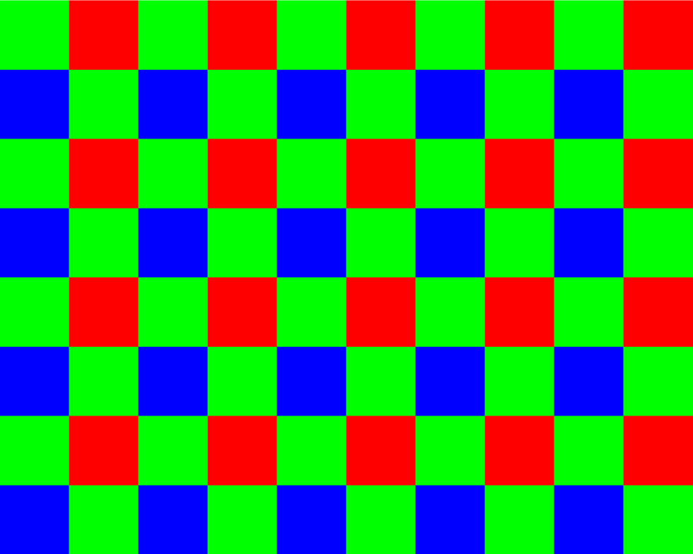
(b) Camera Bayer CFA

Figure 6: Image displayed on a LCD or captured by a camera is spatially resampled in order to achieve color effects.

Considering the drawbacks of using real photos, we employ synthetic screenshot images with realistic moiré patterns for training instead. The input images of the synthesizer are collected by using the print-screen command from computers running Microsoft Windows. To accurately simulate the formation of moiré patterns, we follow truthfully the process of image display on an LCD and the pipeline of optical image capture and digital processing on a camera.

The corresponding ground truth clean image is generated from the original image using the same projective transformation and lens distortion function as the moiré simulator. Additionally, the ground truth image is also scaled to match the same size of the synthetic camera-captured screen image.

5.2 Training Details

From 1,000 digital screenshot images, we create 60,000 $256\times 256$ pairs of artificial moiré affected patch and its cleaning ground truth using the above data synthesizer. Same as the previous experiment, of the 60,000 patches 40,000 are used for training, 10,000 are for validation; and another 10,000 are for testing. For training the proposed DM-Net, we use $10^{5}$ update iterations and a batch size of 32, and we also employ Adam’s optimization method [7] with $\beta_{1}=0.9$ and a learning rate of $10^{-4}$. To deal with the multiple scales, the loss function of DM-Net is set as,

$$L_{\ell_{2}}=\frac{1}{wh}\|g_{0}(y_{s})-x\|_{2}^{2}+\frac{1}{WH}\|G_{0}(Y_{s})-X\|_{2}^{2},$$ (8)

where the $x$ is the downsampled version of $X$, and $w,h$ are the corresponding width and height. The training of DnCNN and RED-Net follows the settings recommended by the original authors.

Using the proposed two-stage training approach, we retrain DM-Net with real moiré images to get a improved version, namely DM-Net+. The training input images for DM-Net+ are real screen images captured using 3 different smartphones (iPhone 6, iPhone 8, Samsung Galaxy S8) from various distances and angles. From the total 300 captured images, 10,000 $256\times 256$ patches are extracted and used as the real degraded input $Y$ in the second training stage. Similar to the previous super-resolution experiment, the network is trained with $10^{4}$ update iterations at a learning rate of $10^{-5}$ in this stage. The time required for the second training stage is much less than the time for the first stage.

For DnCNN and RED-Net, we retrain them using the two-stage approach with the same configuration as DM-Net+. As an attempt to further improve their performances, we extend our training approach to more stages. In every stage, the surrogate ground truth is regenerated using the model from previous stage. Effectively, this method could push the results closer to the distribution of the sample clean images after each stage, due to the minimization of adversarial loss. But it can also deviate the results from the degradation model, making them appear dissimilar to the original images.

5.3 Experimental Results

(a) Input

(b) RED-Net

(c) DnCNN

(d) DM-Net

Figure 7: Results of demoiréing techniques for synthetic moiré images.

Shown in Fig. 7 is the results of the tested techniques for synthetic input. The average PSNRs for DnCNN, RED-Net and DM-Net are 37.46 dB, 37.80 dB and 40.01 dB, respectively. Both DnCNN and RED-Net fail to remove the artifacts completely, leaving traces of wide color bands. In comparison, the output of DM-Net looks much cleaner. As demonstrated by these results, the demoiréing problem is quite challenging; only purposefully designed technique can solve it successfully.

(a) Input

(b) DM-Net

(c) DM-Net+

(d) RED-Net

(e) RED-Net+

(f) DnCNN

(g) DnCNN+

Figure 8: Results of demoiréing techniques for real moiré images.

(a) RED-Net++

(b) RED-Net+++

(c) RED-Net++++

(d) DnCNN++

(e) DnCNN+++

(f) DnCNN++++

Figure 9: Results of RED-Net and DnCNN using 3-stage, 4-stage and 5-stage training.

However, as shown in Figure 8, DM-Net, which achieves excellent performance on the synthetic data, fails to obtain the same quality results for real camera-captured screen images. In contrast, the improved network DM-NET+ works much better for real input images, leaving almost no artifacts. The refined models RED-Net+ and DnCNN+ also make some significant improvements over the original versions without any change to their architectures. However, their results for real images are still relatively noisy in comparison with the results of DM-NET+. After all, the architectures of the two networks are not designed specifically for the demoiré task. We can further improve RED-Net+ and DnCNN+, to some extent, using more training stages as discussed previously. Shown in Figure 9 are some of the results. With more training stages, the results become cleaner but also blurrier in general.

6 Conclusion

In many applications of deep learning, we have to resort to synthesized paired data to train the DCNN, due to the lack of real data. However, the most likely scenario for a deep learning restoration system is that the pairs of the latent and degraded images can only be generated to a limited precision. These paired images, although being flawed, are still valuable initial training data to lay a basis for supervised deep learning, as in current practice. In this work, we are not contented as others with the expediency of artificial training data, and instead strive to correct the deficiency of the existing methods by assuming an overly simplified degradation process. Our main contribution is a more general and robust neural network training approach that can withstand the discrepancies between the synthesized degraded images for training and the actual input images.

References

- [1] J. Anaya and A. Barbu. Renoir–a dataset for real low-light image noise reduction. Journal of Visual Communication and Image Representation, 51:144–154, 2018.
- [2] J. Chen, J. Chen, H. Chao, and M. Yang. Image blind denoising with generative adversarial network based noise modeling. In Proceedings of the IEEE Conference on Computer Vision and Pattern Recognition, pages 3155–3164, 2018.
- [3] Y. Chen, W. Yu, and T. Pock. On learning optimized reaction diffusion processes for effective image restoration. In Proceedings of the IEEE conference on computer vision and pattern recognition, pages 5261–5269, 2015.
- [4] I. Goodfellow, J. Pouget-Abadie, M. Mirza, B. Xu, D. Warde-Farley, S. Ozair, A. Courville, and Y. Bengio. Generative adversarial nets. In Advances in neural information processing systems, pages 2672–2680, 2014.
- [5] S. Gross and M. Wilber. Training and investigating residual nets. Facebook AI Research, CA.[Online]. Avilable: http://torch. ch/blog/2016/02/04/resnets. html, 2016.
- [6] S. Guo, Z. Yan, K. Zhang, W. Zuo, and L. Zhang. Toward convolutional blind denoising of real photographs. arXiv preprint arXiv:1807.04686, 2018.
- [7] D. Kinga and J. B. Adam. A method for stochastic optimization. In International Conference on Learning Representations (ICLR), 2015.
- [8] C. Ledig, L. Theis, F. Huszár, J. Caballero, A. Cunningham, A. Acosta, A. Aitken, A. Tejani, J. Totz, Z. Wang, et al. Photo-realistic single image super-resolution using a generative adversarial network. arXiv preprint, 2016.
- [9] B. Lim, S. Son, H. Kim, S. Nah, and K. M. Lee. Enhanced deep residual networks for single image super-resolution. In The IEEE conference on computer vision and pattern recognition (CVPR) workshops, volume 1, page 4, 2017.
- [10] X. Mao, C. Shen, and Y.-B. Yang. Image restoration using very deep convolutional encoder-decoder networks with symmetric skip connections. In Advances in neural information processing systems, pages 2802–2810, 2016.
- [11] B. Mildenhall, J. T. Barron, J. Chen, D. Sharlet, R. Ng, and R. Carroll. Burst denoising with kernel prediction networks. In Proceedings of the IEEE Conference on Computer Vision and Pattern Recognition, pages 2502–2510, 2018.
- [12] S. Nah, T. H. Kim, and K. M. Lee. Deep multi-scale convolutional neural network for dynamic scene deblurring. In CVPR, volume 1, page 3, 2017.
- [13] S. Roth. Benchmarking denoising algorithms with real photographs.
- [14] A. Shocher, N. Cohen, and M. Irani. Zero-shot” super-resolution using deep internal learning. arXiv preprint arXiv:1712.06087, 2017.
- [15] J. Xu, H. Li, Z. Liang, D. Zhang, and L. Zhang. Real-world noisy image denoising: A new benchmark. arXiv preprint arXiv:1804.02603, 2018.
- [16] Z. Yi, H. R. Zhang, P. Tan, and M. Gong. Dualgan: Unsupervised dual learning for image-to-image translation. In ICCV, pages 2868–2876, 2017.
- [17] K. Zhang, W. Zuo, Y. Chen, D. Meng, and L. Zhang. Beyond a gaussian denoiser: Residual learning of deep cnn for image denoising. IEEE Transactions on Image Processing, 26(7):3142–3155, 2017.
- [18] J.-Y. Zhu, T. Park, P. Isola, and A. A. Efros. Unpaired image-to-image translation using cycle-consistent adversarial networks. In Computer Vision (ICCV), 2017 IEEE International Conference on, pages 2242–2251. IEEE, 2017.