State dependent spread of entanglement in relatively local Hamiltonians

Abstract

Relatively local Hamiltonians are a class of background independent non-local Hamiltonians from which local theories emerge within a set of short-range entangled states. The dimension, topology and geometry of the emergent local theory is determined by the initial state to which the Hamiltonian is applied. In this paper, we study dynamical properties of a simple relatively local Hamiltonian for $N$ scalar fields in the large $N$ limit. It is shown that the coordinate speeds at which entanglement spreads and local disturbance propagates in space strongly depend on state in the relatively local Hamiltonian.

I Introduction

Locality, one of the cherished principles in quantum field theoryWichmann and Crichton (1963), is unlikely to be a part of the yet unknown fundamental theory of nature that includes dynamical gravityMarolf (2015). In the presence of strong quantum fluctuations of metric, there is no well-defined notion of what is near and what is far. At the same time, a quantum theory of gravity that reproduces the general relativity in the classical limit can not be a generic non-local theory either. If quantum fluctuation of geometry is weak, a local field theory should emerge as an effective description of quanta propagating on top of the classical geometry that describes a saddle point of the fundamental theory. In this case, locality defined with respect to the saddle point geometry is determined by the state not by the fundamental Hamiltonian. One possibility is that the microscopic theory that includes gravity belongs to a class of non-local theories which act approximately as local theories within a set of states that represent classical geometry. Such theories, while being non-local in the usual sense, must have a weaker sense of locality. We call it relative locality that locality of Hamiltonian is determined relative to state.

Recently, it has been argued that the general relativity can arise as a semi-classical description of a relatively local quantum theory of matter fieldsLee (2018). In the construction, spatial metric is introduced as a collective variable that characterizes how matter fields are entangled in space within a sub-Hilbert space. One can design a Hamiltonian for the matter fields such that it induces the classical general relativity for the collective variable at long distances in the limit that the number of matter fields is large. The Hamiltonian is shown to have the property that the range of interactions depends on the entanglement present in states on which the Hamiltonian acts. Although the theory is non-local in the strict sense, it differs from generic non-local theoriesSachdev and Ye (1993); Kitaev (2015) in that a local effective theory emerges in a space of short-range entangled states. In the theory, the notion of distance that sets locality of Hamiltonian is determined by entanglement present in state. In relatively local theories, the relation between entanglement and geometryRyu and Takayanagi (2006); Hubeny et al. (2007); Van Raamsdonk (2010); Casini et al. (2011); Lewkowycz and Maldacena (2013) uncovered in the context of AdS/CFT correspondenceMaldacena (1999); Witten (1998); Gubser et al. (1998) is promoted to a kinematic principle that posits that geometry is a collective degree of freedom that encodes entanglement of matter fields. In this sense, relatively local theories can be viewed as examples of emergent gravity that realize the $ER=EPR$ conjectureMaldacena and Susskind (2013).

However, the relatively local theory introduced in Ref. Lee (2018) is defined only perturbatively in the semi-classical limit. The construction starts with matter fields defined on a manifold with a fixed dimension and topology, and it is not capable of describing non-perturbative processes. Furthermore, the continuum Hamiltonian of the matter fields is rather complicated, and its dynamics hasn’t been studied explicitly. Therefore it is of interest to consider tractable relatively local models that can be defined beyond the perturbative level. In this paper, we construct a simple relatively local Hamiltonian for $N$ scalar fields, and study its dynamics in the large $N$ limit.

Here is the outline of the paper. In Sec. II, we define the Hilbert space and the Hamiltonian. Sec. II A starts with the Hilbert space of $N$ scalar fields which are defined on a collection of sites. Within the full Hilbert space, we focus on a sub-Hilbert space that is invariant under an internal symmetry group. The symmetric sub-Hilbert space is spanned by basis states which are labeled by multi-local singlet collective variables. In Sec. II B we introduce a relatively local Hamiltonian that is invariant not only under the internal symmetry but also under the full permutation group of the sites. The relatively local Hamiltonian has no preferred background, and is non-local as a quantum operator. However, it acts as a local Hamiltonian within a set of states with local structures of entanglement in the large $N$ limit. A state is said to have a local structure of entanglement (henceforth called ‘local structure’, in short) if entanglement entropy of any sub-region can be written as the volume of its boundary measured with a classical notion of distance (metric) associated with a lattice (manifold). The existence of such a lattice, and the dimension, topology and geometry of the lattice, if exists, are all determined by the pattern of entanglement of state. The lattice associated with a state with a local structure consequently determine the dimension, topology and geometry of the local theory that emerges when the Hamiltonian is applied to that state. In this sense, the locality of the Hamiltonian is set by states. In Sec. III, we study time evolution of states with local structures. We derive an induced Hamiltonian for the collective variables that governs the time evolution of states within the symmetric sub-Hilbert space. In the large $N$ limit, the time evolution is described by classical equations of motion for the collective variables. Sec. III A is devoted to the perturbative analysis that describes time evolution of states which are close to direct product states. It treats small entanglement as a perturbation added to an unentangled ultra-local state. It is shown that the coordinate speed at which entanglement spreads in space vanishes in the limit that the entanglement of the initial state vanishes. In Sec. III B, we numerically integrate the classical equation of motion for the collective variables. We confirm that the coordinate speed at which entanglement spreads depends strongly on the amount of entanglement in the initial state. Furthermore, it is shown that the local structure of the initial state determines the dimension of the emergent local theory. In Sec. IV, we examine propagation of a local disturbance added to a translationally invariant initial state. It is shown that a small local disturbance propagates on top of the geometry set by the collective variables that are formed in the absence of the disturbance. The coordinate speed of the propagating mode is determined by the initial state because the geometry is set by the state.

II Model

II.1 Hilbert space

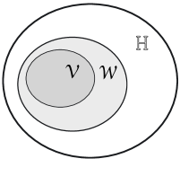
Figure 1: ${\mathbb{H}}$ is the full Hilbert space of the scalar fields. ${\cal W}$ is the $S_{N}\ltimes Z_{2}^{N}$ invariant sub-Hilbert space of ${\mathbb{H}}$. ${\cal V}$ is the $O(N)$ invariant sub-Hilbert space of ${\cal W}$.

We first introduce the Hilbert space in which our model is defined. We consider a quantum system defined on a set of sites labeled by $i=1,2,..,L$. At each site, there are $N$ real scalar fields $\phi_{i}^{a}$ with $a=1,2,..,N$. The full Hilbert space is spanned by the basis states $\Bigl{\{}\big{|}\phi\big{>}\big{|}-\infty<\phi^{a}_{i}<\infty\Bigr{\}}$, where $\big{|}\phi\big{>}$ is the eigenstate of the field operator that satisfies $\hat{\phi}^{a}_{i}\big{|}\phi\big{>}=\phi^{a}_{i}\big{|}\phi\big{>}$ and $\big{<}\phi^{\prime}\big{|}\phi\big{>}=\prod_{i,a}\delta\left(\phi_{i}^{{}^{\prime}a}-\phi_{i}^{a}\right)$. Within the full Hilbert space, we consider the $S_{N}\ltimes Z_{2}^{N}$ invariant sub-Hilbert space denoted as ${\cal W}$. Here $S_{N}$ is the global flavor permutation group under which the field transforms as $\phi_{i}^{a}\rightarrow\phi_{i}^{P_{a}}$. Under each of the $N$ independent $Z_{2}$ transformations, one component of the scalar field flips sign as $\phi_{i}^{a}\rightarrow(-1)^{\delta_{ab}}\phi_{i}^{a}$ with $b=1,2,..,N$. $S_{N}\ltimes Z_{2}^{N}$ is a subgroup of the $O(N)$ group. General wavefunctions in ${\cal W}$ can be written as functions of multi-local single-trace operators with even powers,

$$O_{i_{1}i_{2}..i_{2n}}\equiv\frac{1}{N}\sum_{a}\phi^{a}_{i_{1}}\phi^{a}_{i_{2}}...\phi^{a}_{i_{2n}}.$$ (1)

This is because $\{O_{i_{1}i_{2}..i_{2n}}\}$ forms a complete basis for the polynomials of the fundamental fields that are invariant under $S_{N}\ltimes Z_{2}^{N}$. Consequently, ${\cal W}$ can be spanned by basis states,

$$\big{|}{\cal T}\big{>}=\int D\phi~{}e^{-N\sum_{n}T_{i_{1}i_{2}..i_{2n}}O_{i_{1}i_{2}..i_{2n}}}\big{|}\phi\big{>},$$ (2)

where $D\phi\equiv\prod_{i,a}d\phi^{a}_{i}$. Henceforth, repeated site indices are understood to be summed over all sites unless mentioned otherwise. The set of symmetric complex tensors of even ranks, ${\cal T}=\Bigl{\{}T_{ij},T_{ijkl},...\Bigr{\}}$ are collective variables that label basis states of ${\cal W}$. The subset of states with pure imaginary collective variables, $\Bigl{\{}\big{|}{\cal T}\big{>}~{}|~{}T_{i_{1}i_{2}..i_{2n}}=it_{i_{1}i_{2}..i_{2n}},~{}t_{i_{1}i_{2}..i_{2n}}\in\mathbb{R}\Bigr{\}}$ is already a complete basis of ${\cal W}$. This follows from the fact that $t_{i_{1}i_{2}..i_{2n}}$ is the Fourier conjugate variable of $O_{i_{1}i_{2}..i_{2n}}$. Therefore, general states in ${\cal W}$ can be expressed as

$$\big{|}\chi\big{>}=\int D{\cal T}~{}\big{|}{\cal T}\big{>}\chi({\cal T}),$$ (3)

where $D{\cal T}\equiv\prod_{i\geq j}dT_{ij}\prod_{i\geq j\geq k\geq l}dT_{ijkl}...$, and the integration over $T_{i_{1}i_{2}..i_{2n}}$ is defined along the imaginary axis. $\chi({\cal T})$ is a wavefunction for the collective variables. Although it is defined on the imaginary axes of ${T_{i_{1}i_{2}..i_{2n}}}$’s, it is useful to analytically extend $\big{|}{\cal T}\big{>}$ and $\chi({\cal T})$ to the complex planes for the following reasons. First, $\big{|}{\cal T}\big{>}$ is not normalizable if $T_{i_{1}i_{2}..i_{2n}}$ is pure imaginary, and one should add a real symmetric tensor $e_{i_{1}i_{2}..i_{2n}}$ to construct normalizable states. Real components of the tensors create normalizable wave-packets. Second, $\chi({\cal T})$ has saddle points off the imaginary axes in general, and one needs to deform the path of $\int dT_{i_{1}i_{2}..i_{2n}}$ in the complex planes for the saddle-point approximation. Within ${{\cal W}}$ there is a sub-space ${\cal V}$ that is $O(N)$ symmetric. Among all multi-local single-trace operators in Eq. (1), only bi-local operators are invariant under the $O(N)$ transformations. Therefore, ${\cal V}$ is spanned by $\big{|}{\cal T}\big{>}$ with $T_{i_{1}i_{2}..i_{2n}}=0$ for $n\geq 2$. We denote basis states of ${\cal V}$ as $\big{|}T\big{>}$ which is labeled by $T_{ij}$ only. This is illustrated in Fig. 1. ${\cal V}$ will be the main focus of the present work.

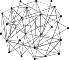
Figure 2: A set of sites connected by bi-local collective variables, where the thickness of the bond between $i,j$ represents the magnitude of $T_{ij}$. For generic choices of bi-local fields, graphs do not represent regular lattices.

The collective variables are a direct measure of entanglement. For a state $\big{|}T\big{>}$ in ${\cal V}$ with $|T_{i\neq j}|\ll e_{ii},e_{jj}$ where $T_{ij}=e_{ij}+it_{ij}$, the entanglement entropy between a subset of sites $A$ and its compliment $\bar{A}$ is given byLee (2016)

$$S_{A}=N\left[\sum_{i\in A,j\in\bar{A}}\left(-\ln\frac{|T_{ij}|^{2}}{4e_{ii}e_{jj}}+1\right)\frac{|T_{ij}|^{2}}{4e_{ii}e_{jj}}+O\left((T/e)^{4}\right)\right]+O(N^{0}).$$ (4)

To the second order in $T_{ij}$, the mutual information between sites $i$ and $j$ is $I_{ij}=N\left(-\ln\frac{|T_{ij}|^{2}}{4e_{ii}e_{jj}}+1\right)\frac{|T_{ij}|^{2}}{4e_{ii}e_{jj}}+O(N^{0})$ . It is useful to visualize the mutual informations between sites in terms of entanglement bonds as is shown in Fig. 2. A notion of distance between sites can be defined based on entanglementCao et al. (2017). For example, one can define a distance between sites $i$ and $j$ as a function of the bi-local fields such that sites that can be connected by few strong bonds have a small proper distance, and sites that can only be connected by many weak bonds have a large proper distance. One such distance function that captures this idea in the limit that $|T_{ij}|$ is small is $\min_{C}\left[-\sum_{(l,m)\in C}\ln|T_{lm}|^{2}\right]$ where $C$ denotes chains of bi-local fields that connect $i$ and $j$.

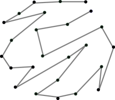
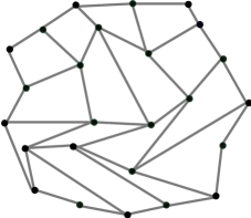
Figure 3: Entanglement bonds that exhibit one and two dimensional local structures, respectively.

Graphs that emerge from random choices of $T_{ij}$ do not represent any lattice in general. There exists a special set of states whose entanglement bonds exhibit a lattice with a sense of locality. We define that a state has a local structure if the entanglement entropy of any sub-region is proportional to the volume of its boundary defined with respect to a lattice. Whether there exists such lattice or not is a property of states. A local structure arises if the pattern of entanglement exhibits a sense of locality. For example, $T_{ij}(0)=\delta_{ij}+\epsilon\delta_{d_{ij}^{(1)},1}$ with $d_{ij}^{(1)}=[i-j]_{L}$ and $[x]_{L}=min\left\{|x+nL|\Big{|}n\in\mathbb{Z}\right\}$ describes the one-dimensional lattice with nearest neighbor bonds and the periodic boundary condition. A torus of $\sqrt{L}\times\sqrt{L}$ square lattice arises in states with $T_{ij}(0)=\delta_{ij}+\epsilon\delta_{d_{ij}^{(2)},1}$ and $d_{ij}^{(2)}=\sqrt{\left[i-j\right]_{\sqrt{L}}^{2}+\left[\left\|\frac{i-1}{\sqrt{L}}\right\|-\left\|\frac{j-1}{\sqrt{L}}\right\|\right]_{\sqrt{L}}^{2}}$, where $\left\|x\right\|$ represents the largest integer equal to or smaller than $x$. The entanglement bonds with one and two dimensional local structures are shown in Fig. 3. Here, the dimension, topology and geometry of the emergent lattice are properties of states determined by the collective variable. In the thermodynamic limit, ${\cal V}$ includes states that describe any lattice in any dimension.

II.2 Relatively Local Hamiltonian

Now we construct a relatively local Hamiltonian whose dimension, topology and locality are determined by those of states. For this, we can not have a local hopping term that is based on a pre-determined notion of distance. Instead, the range and the strength of hopping need to be state dependent. Here we consider a simple relatively local Hamiltonian that is invariant under $S_{N}\ltimes Z_{2}^{N}$,

$$\hat{H}=-R\sum_{i,j}\sum_{a}\hat{T}_{ij}^{a}(\hat{\phi}_{i}^{a}\hat{\phi}_{j}^{a})+U\sum_{i}\sum_{a}\hat{\pi}_{i}^{a}\hat{\pi}_{i}^{a}+\frac{\lambda}{N}\sum_{i}\sum_{a,b}(\hat{\phi}_{i}^{a}\hat{\phi}_{i}^{a})(\hat{\phi}_{i}^{b}\hat{\phi}_{i}^{b}).$$ (5)

Here $R$, $U$, $\lambda$ are constants, and $\hat{\pi}_{i}^{a}$ is the conjugate momentum of $\hat{\phi}_{i}^{a}$. The second and the third are the standard kinetic and quartic interaction terms that are ultra-local. The first term describes ‘hoppings’. If the hopping was nonzero only between nearby sites in a fixed lattice, this Hamiltonian would be a usual local Hamiltonian. The key differences of Eq. (5) from such local Hamiltonians are that $i,j$ run over all pairs of sites, and the hopping amplitude is an operator. The strength of hopping between two sites is determined by $\hat{T}_{ij}^{a}$ which measures inter-site entanglement bonds. Since there can be potentially nonzero coupling between any two sites, $\hat{H}$ is a non-local Hamiltonian as a quantum operator. However, $\hat{T}_{ij}^{a}$ can be chosen such that $\hat{H}$ acts as a local Hamiltonian within states that have local structures.

Because $T_{ij}$ is the collective variable that determines pairwise connectivity, one may try to construct $\hat{T}_{ij}^{a}$ such that $\hat{T}_{ij}^{a}\big{|}T\big{>}=T_{ij}\big{|}T\big{>}$. However, it is not easy to find such operator because not all states with different collective variables are linearly independent for $L\gg N$. Alternatively, we look for an operator of which $\big{|}T\big{>}$ is an approximate eigenstate. One such operator that commutes with $\hat{\phi}_{i}^{a}\hat{\phi}_{j}^{a}$ is

$$\hat{T}_{ij}^{a}=\frac{1}{N-1}\sum_{b\neq a}\hat{\pi}_{i}^{b}\hat{\pi}_{j}^{b}.$$ (6)

For states in ${\cal V}$, the operator satisfies

$$\hat{T}_{ij}^{a}\big{|}T\big{>}=\int D\phi~{}\left[2T_{ij}-4T_{ik}T_{lj}\frac{\sum_{b\neq a}\phi_{k}^{b}\phi_{l}^{b}}{N-1}\right]e^{-NT_{ij}O_{ij}}\big{|}\phi\big{>}.$$ (7)

While $\big{|}T\big{>}$ is not an eigenstate of $\hat{T}_{ij}$, its expectation value is given by

$$\frac{\big{<}T\big{|}\hat{T}_{ij}\big{|}T\big{>}}{\big{<}T\big{|}T\big{>}}=2(T^{*-1}+T^{-1})^{-1}_{ij}.$$ (8)

Here $T_{ij}^{-1}$ denotes the inverse of $T_{ij}$ as an $L\times L$ matrix. Eq. (8) reduces to $T_{ij}$ for real $T_{ij}$. $\hat{T}_{ij}^{a}$ is an operator that measures the strength of the bond between $i$ and $j$. Therefore, $-\hat{T}_{ij}^{a}\hat{\phi}_{i}^{a}\hat{\phi}_{j}^{a}$ represents hoppings between all pairs of sites with strength proportional to the pre-existing entanglement between the sites. It is noted that Eq. (5) has the full permutation symmetry of $L$ sites. The permutation group includes the usual discrete translational symmetry of any regular lattice as subgroups, and the Hamiltonian does not have a preferred background.

$\hat{T}_{ij}$ is a quantum operator that measures the geometry of states. In quantum mechanics, it is in general impossible to read information without disturbing the stateBus (1996). However, $\hat{T}_{ij}$ acts as a classical variable to the leading order in $1/N$ when applied to semi-classical states. This is attributed to the fact that the geometric information is encoded redundantly by a large number of matter fields in the large $N$ limit. To see this, we consider a general state in Eq. (3) with a semi-classical wavefunction for the collective variables,

$$\chi({\cal T}) = e^{\sum_{n}\left[N\bar{P}_{i_{1}i_{2}..i_{2n}}\left(T_{i_{1}i_{2}..i_{2n}}-\bar{T}_{i_{1}i_{2}..i_{2n}}\right)+\frac{\left(T_{i_{1}i_{2}..i_{2n}}-\bar{T}_{i_{1}i_{2}..i_{2n}}\right)^{2}}{2\Delta^{2}}\right]},$$ (9)

where $\bar{T}_{i_{1}i_{2}..i_{2n}}$ and $\bar{P}_{i_{1}i_{2}..i_{2n}}$ denote classical collective variables and their conjugate momenta, respectively. Eq. (9) is a normalizable wavefunction with width $\Delta$ defined along the imaginary axes of $T_{i_{1}i_{2}..i_{2n}}$’s. For $1/N\ll\Delta\ll 1$, both the collective variables and their conjugate momenta are well defined. For simplicity, let us consider states with $\bar{T}_{i_{1}i_{2}..i_{2n}}(t)=\bar{P}_{i_{1}i_{2}..i_{2n}}(t)=0$ for $n\geq 2$. Application of $\hat{T}_{ij}$ to the semi-classical state leads to

$$\hat{T}_{ij}\big{|}\chi\big{>} \approx \left[2\bar{T}_{ij}-4\bar{T}_{ik}\bar{P}_{kl}\bar{T}_{lj}\right]\big{|}\chi\big{>}$$ (10)

to the leading order in $1/N$ and $\Delta$. Here we use Eq. (7) and $\int D{{\cal T}}~{}(\sum_{b}\hat{\phi}_{k}^{b}\hat{\phi}_{l}^{b})~{}\big{|}{{\cal T}}\big{>}\chi({{\cal T}})=\int D{{\cal T}}~{}\big{|}{{\cal T}}\big{>}\left(-i\frac{\partial}{\partial t_{kl}}\right)\chi({{\cal T}})$. The latter relation implies that $\sum_{b}\hat{\phi}_{k}^{b}\hat{\phi}_{l}^{b}\sim N\bar{P}_{kl}$ plays the role of the conjugate momentum. Therefore, $\hat{T}_{ij}$ acts as a classical variable in the space of semi-classical states. This is true for more general semi-classical states in which higher order multi-local fields are turned on. If $\bar{T}_{ij}$ and $\bar{P}_{ij}$ decay in a distance function $d_{ij}$ associated with a lattice, the state exhibits a local structure. In this case, $\hat{T}_{ij}\big{|}\chi\big{>}$ also decays exponentially following the local structure of the state, and Eq. (5) is well approximated by a local Hamiltonian. For example, only one-dimensional local hopping terms survive to the leading order in $1/N$ if the Hamiltonian is applied to $\big{|}\chi\big{>}$ with $\hat{T}_{ij}\big{|}\chi\big{>}=\left[e^{-[i-j]_{L}/\xi}+O(1/N)\right]\big{|}\chi\big{>}$.

Now we examine time evolution of states in ${\cal W}$ generated by $\hat{H}$. An application of $e^{-idt\hat{H}}$ to $\big{|}{\cal T}\big{>}$ leads to

$$e^{-idt\hat{H}}\big{|}{\cal T}\big{>}=\int D\phi~{}e^{-idtN{\cal H}_{0}\left[{\cal T},{\cal O}\right]}~{}e^{-N\sum_{n}T_{i_{1}i_{2}..i_{2n}}O_{i_{1}i_{2}..i_{2n}}}\big{|}\phi\big{>},$$ (11)

where ${\cal H}_{0}[{\cal T},{\cal O}]$ is the induced Hamiltonian,

$${\cal H}_{0}[{\cal T},{\cal O}]=$$

$$-R^{\prime}\Bigl{[}\sum_{n}2n(2n-1)T_{ijj_{1}j_{2}..j_{2n-2}}O_{ij}O_{j_{1}j_{2}..j_{2n-2}}-\sum_{n,m}4nmT_{jj_{1}j_{2}..j_{2n-1}}T_{ii_{1}i_{2}..i_{2m-1}}O_{ij}O_{j_{1}j_{2}..j_{2n-1}i_{1}i_{2}..i_{2m-1}}\Bigr{]}$$

$$+U\Bigl{[}\sum_{n}2n(2n-1)T_{iij_{1}j_{2}..j_{2n-2}}O_{j_{1}j_{2}..j_{2n-2}}-\sum_{n,m}4nmT_{ij_{1}j_{2}..j_{2n-1}}T_{ii_{1}i_{2}..j_{2m-1}}O_{j_{1}j_{2}..j_{2n-1}i_{1}i_{2}..i_{2m-1}}\Bigr{]}+\lambda O_{ii}^{2}$$

$$+\frac{R^{\prime}}{N}\Bigl{[}\sum_{n}2n(2n-1)T_{ijj_{1}j_{2}..j_{2n-2}}O_{ijj_{1}j_{2}..j_{2n-2}}-\sum_{n,m}4nmT_{jj_{1}j_{2}..j_{2n-1}}T_{ii_{1}i_{2}..i_{2m-1}}O_{ijj_{1}j_{2}..j_{2n-1}i_{1}i_{2}..i_{2m-1}}\Bigr{]}\Biggr{\}}$$

(12)

with $R^{\prime}=\frac{N}{N-1}R$. Because $\{\big{|}{\cal T}\big{>}\}$ is a complete basis of ${\cal W}$, Eq. (11) can be written as a linear superposition of $\big{|}{\cal T}\big{>}$,

$$e^{-idt\hat{H}}\big{|}\chi\big{>} = \int D{\cal T}^{(1)}D{\cal P}^{(1)}D{\cal T}^{(0)}~{}\big{|}{\cal T}^{(1)}\big{>}~{}e^{N\sum_{n}P_{i_{1}i_{2}..i_{2n}}^{(1)}\left(T_{i_{1}i_{2}..i_{2n}}^{(1)}-T_{i_{1}i_{2}..i_{2n}}^{(0)}\right)-iNdt{\cal H}_{0}[{\cal T}^{(0)},{\cal P}^{(1)}]}~{}\chi({\cal T}^{(0)}),$$

where ${\cal H}_{0}[{\cal T},{\cal P}]$ is given by Eq. (12) with ${\cal O}$ replaced with ${\cal P}$. The integration $T^{(1)}_{i_{1}i_{2}..i_{2n}}$ in Eq. (LABEL:ieH) is defined along the imaginary axis in the complex plane, where $\int D{\cal T}^{(1)}\equiv\int_{-\infty}^{\infty}\prod_{i\geq j}dt_{ij}^{(1)}\prod_{i\geq j\geq k\geq l}dt_{ijkl}^{(1)}..$ with $T_{i_{1}i_{2}..i_{2n}}^{(1)}=it_{i_{1}i_{2}..i_{2n}}^{(1)}$. On the contrary, the integration over ${\cal P}$ is defined along the real axis. One can readily see that the integration over $t_{i_{1}i_{2}..i_{2n}}^{(1)}$ gives rise to the delta function, $\delta\left(P^{(1)}_{i_{1}i_{2}..i_{2n}}-O_{i_{1}i_{2}..i_{2n}}\right)$. The following integration of ${\cal P}$ reproduces Eq. (11).

A finite time evolution is given by a path integration over the collective variables and their conjugate momenta,

$$e^{-it\hat{H}}\big{|}\chi\big{>} = \int{\cal D}{\cal T}{\cal D}{\cal P}~{}\big{|}{\cal T}(t)\big{>}~{}e^{iS[{\cal T},{\cal P}]}~{}\chi({\cal T}(0)),$$ (14)

where

$$S[{\cal T},{\cal P}] = N\int_{0}^{t}d\tau\Bigl{[}-i\sum_{n}P_{i_{1}i_{2}..i_{2n}}\partial_{\tau}T_{i_{1}i_{2}..i_{2n}}-{\cal H}_{0}[{\cal T},{\cal P}]\Bigr{]},$$ (15)

and ${\cal D}{\cal T}{\cal D}{\cal P}\equiv\prod_{s=0}^{M_{t}}D{\cal T}^{(s)}\prod_{s=1}^{M_{t}}D{\cal P}^{(s)}$ with $M_{t}=t/dt$ and $\tau=s~{}dt$. The factor of $-i$ in Eq. (15) is the reminder that $T_{i_{1}i_{2}..i_{2n}}$ should be integrated along the imaginary axes in the path integration. It is noted that $-iT_{i_{1}i_{2}..i_{2n}}$ and $P_{i_{1}i_{2}..i_{2n}}$ are conjugate to each other. Although ${\cal H}_{0}$ is not Hermitian, it is $PT$-symmetric under which $t_{i_{1}i_{2}..i_{2n}}\rightarrow-t_{i_{1}i_{2}..i_{2n}}$, $P_{i_{1}i_{2}..i_{2n}}\rightarrow P_{i_{1}i_{2}..i_{2n}}$Bender et al. (1999); Lee (2016). ${\cal H}_{0}$ also has a real spectrum because the original Hamiltonian in Eq. (5) is Hermitian. ${\cal H}_{0}$ can be mapped to a Hermitian Hamiltonian through a similarity transformation. However, we will proceed with the current representation of the Hamiltonian.

III State dependent spread of entanglement

III.1 Perturbative analysis near ultra-local solution

Figure 4: The contours of the path integrations in the complex planes of $T_{i_{1}i_{2}..i_{2n}}$ and $P_{i_{1}i_{2}..i_{2n}}$. While the original paths (solid lines) are defined along the imaginary and real axes respectively, the saddle points in general lie away from the original paths. The saddle point can be reached by deforming the paths as denoted in the dashed lines. Fluctuations around the saddle point are defined along the deformed paths.

In this section, we examine time evolution of semi-classical states in Eq. (9). In the large $N$ limit, the path integration in Eq. (14) is dominated by the saddle point path which satisfies the classical equation of motion. While the integrations for $T_{i_{1}i_{2}..i_{2n}}$ and $P_{i_{1}i_{2}..i_{2n}}$ in Eq. (14) are defined along the imginary and the real axes respectively, they take general complex values at a saddle point. This is illustrated in Fig. 4.

For general initial states in ${\cal W}$, one should include all multi-local collective variables in the saddle-point solution. Here we consider initial states with $\bar{T}_{i_{1}i_{2}..i_{2n}}=0$ and $\bar{P}_{i_{1}i_{2}..i_{2n}}=0$ for $n\geq 2$. When only bi-local collective fields are turned on at $t=0$, $T_{i_{1}i_{2}..i_{2n}}(t)=0$ at all $t$ for $n\geq 2$ to the leading order in $1/N$. This is due to the fact that the initial state in ${\cal V}$ has the $O(N)$ symmetry, and the Hamiltonian in Eq. (5) also respects the $O(N)$ symmetry to the leading order in $1/N$. Multi-local fields break the $O(N)$ symmetry, and they are not generated to the leading order in $1/N$. With $T_{i_{1}i_{2}..i_{2n}}(t)=0$ for $n\geq 2$, the equations of motion for $T_{ij}$ and $P_{ij}$ decouple from $P_{i_{1}i_{2}..i_{2n}}$ with $n\geq 2$ as well. This allows one to use the effective Hamiltonian for the bi-local fields only,

$${\cal H}[T,P] = R\left(-2T_{ij}P_{ji}+4T_{ik}P_{kl}T_{lj}P_{ji}\right)+U\left(2T_{ii}-4T_{ik}P_{kl}T_{li}\right)+\lambda P_{ii}^{2}+O\left(N^{-1}\right),$$ (16)

which is obtained by turning off all multi-local fields with $n\geq 2$ in Eq. (12). The bi-local fields obey the equation of motion,

$$-i~{}\partial_{\tau}T_{ij} = R\left(-2T_{ij}+8T_{ik}P_{kl}T_{lj}\right)-4UT_{ik}T_{kj}+2\lambda P_{ii}\delta_{ij},$$

$$i~{}\partial_{\tau}P_{ij} = R\left(-2P_{ij}+8P_{ik}T_{kl}P_{lj}\right)+U\left(2\delta_{ij}-4P_{ik}T_{kj}-4T_{ik}P_{kj}\right)$$ (17)

with the initial condition $T_{ij}(0)=\bar{T}_{ij}$, $P_{ij}(0)=\bar{P}_{ij}$.

The spectrum of Eq. (5) is bounded neither from above nor from below. However, the time evolution of a closed system with fixed energy is well defined because the energy is conserved. The same is true for the general relativity which has an unbounded spectrum. The full Hilbert space is vast, and most states do not have a local structure. Here we focus on a small fraction of initial states which exhibit local structures. We do not attempt to find a dynamical mechanism that may select such initial states. Instead, our focus is to consider the time evolution of states with local structures, and show that the relatively local Hamiltonian acts as a local theory within the states with local structures.

Let us first consider ultra-local solutions. For $T_{ij}=T_{i}\delta_{ij}$, $P_{ij}=P_{i}\delta_{ij}$, the equation of motion for each site is decoupled from others,

$$-i~{}\partial_{\tau}T_{i} = R\left(-2T_{i}+8T_{i}^{2}P_{i}\right)-4UT_{i}^{2}+2\lambda P_{i},$$

$$i~{}\partial_{\tau}P_{i} = R\left(-2P_{i}+8P_{i}^{2}T_{i}\right)+U\left(2-8P_{i}T_{i}\right).$$ (18)

For $8U^{2}\lambda>R^{3}$, there exists one ultra-local static solution (fixed point) on the real axes of $T_{i}$ and $P_{i}$ : $(T_{*},P_{*})=\left(\frac{1}{2}\left(\frac{\lambda}{U}\right)^{1/3},\frac{1}{2}\left(\frac{U}{\lambda}\right)^{1/3}\right)$. For $8U^{2}\lambda\leq R^{3}$, two more fixed points coalesce on the real axes : $(T_{**}^{+},P_{**}^{+})=\left(\frac{R^{2}+\sqrt{R(R^{3}-8U^{2}\lambda)}}{4UR},\frac{U}{R}\right)$ and $(T_{**}^{-},P_{**}^{-})=\left(\frac{R^{2}-\sqrt{R(R^{3}-8U^{2}\lambda)}}{4UR},\frac{U}{R}\right)$. The static ultra-local solutions describe direct product states. The direct product states remain to be direct product states under the time evolution because the Hamiltonian acts as a ultra-local Hamiltonian within the subspace of states without spatial entanglement.

Figure 5: (a) The initial state in Eq. (19) has only nearest neighbor entanglement bonds. (b) Under time evolution, further neighbor bonds are generated.

Here we focus on the case with $8U^{2}\lambda>R^{3}$, and examine how initial states which are slightly perturbed away from the ultra-local fixed point evolve in time. To be concrete, we consider the initial condition,

$$T_{ij}(0) = T_{*}\delta_{ij}+\epsilon\delta_{d_{ij}^{(1)},1},$$

$$P_{ij}(0) = P_{*}\delta_{ij},$$ (19)

where $d_{ij}^{(1)}=[i-j]_{L}$. The initial condition describes the ultra-local state perturbed with nearest neighbour entanglement bonds with strength $\epsilon$ that forms the one-dimensional lattice with the periodic boundary condition. With the one-dimensional local structure, it is natural to use the label for each site as a coordinate of the lattice. In the small $\epsilon$ limit, the initial state obeys the area law of entanglement : the entanglement entropy of a sub-region scales as $-\epsilon^{2}\ln\epsilon^{2}$, and is independent of the sub-system size to the leading order. The solution in $t>0$ is written as

$$T_{ij}(t) = T_{0,ij}+\epsilon~{}T_{1,ij}(t)+\epsilon^{2}~{}T_{2,ij}(t)+...,$$

$$P_{ij}(t) = P_{0,ij}+\epsilon~{}P_{1,ij}(t)+\epsilon^{2}~{}P_{2,ij}(t)+...~{}~{}.$$ (20)

Here $T_{0,ij}=T_{*}\delta_{ij}$ and $P_{0,ij}=P_{*}\delta_{ij}$ denote the unperturbed ultra-local static solution. Eq. (20) includes higher order terms in $\epsilon$ as well because the non-linearity of the equation of motion generates higher order terms at later time even though the initial condition has only $O(\epsilon)$ perturbation. Under time evolution, the second neighbor and further neighbor bi-local fields are generated, creating longer-range entanglement in the system. This is illustrated in Fig. 5. The increase in the range of the bi-local fields in real space describes how entanglement spreads in space. For earlier studies of spread of entanglement in local and non-local Hamiltonians, see Refs. Nozaki et al. (2013); Jurcevic et al. (2014); Rangamani et al. (2016); Casini et al. (2016); Liu and Suh (2014); Mezei and Stanford (2017); Kundu and Pedraza (2017).

In organizing the equation of motion as a perturbative series in $\epsilon$, it is convenient to combine the phase space variables at each order into a two-component complex vector, $\vec{V}_{n,ij}=\left(\begin{array}[]{c}T_{n,ij}\\ P_{n,ij}\end{array}\right)$. The phase space vectors obey the equations of motion,

$$\partial_{t}\vec{V}_{n,ij} = M_{ij}\vec{V}_{n,ij}+\vec{A}_{n,ij},$$ (21)

where

$$M_{ij} = i\left(\begin{array}[]{cc}-2R+16RT_{*}P_{*}-8UT_{*}&8RT_{*}^{2}+2\lambda\delta_{ij}\\ -8RP_{*}^{2}+8UP_{*}&2R-16RT_{*}P_{*}+8UT_{*}\end{array}\right),$$ (24)

and

$$\vec{A}_{1,ij} = 0,$$

$$\vec{A}_{n,ij} = i\left(\begin{array}[]{c}8R\sum\limits_{a,b,c<n}T_{a,ik}P_{b,kl}T_{c,lj}~{}\delta_{a+b+c,n}-4U\sum\limits_{a,b<n}T_{a,ik}T_{b,kj}~{}\delta_{a+b,n}\\ -8R\sum\limits_{a,b,c<n}P_{a,ik}T_{b,kl}P_{c,lj}~{}\delta_{a+b+c,n}+4U\sum\limits_{a,b<n}(P_{a,ik}T_{b,kj}+T_{a,ik}P_{b,kj})~{}\delta_{a+b,n}\end{array}\right)$$ (27)

for $n>1$. In Eqs. (21) - (27), repeated site indices are summed over all sites except for $i,j$. $M_{ij}$ is the linearized Hamiltonian that dictates the orbit of $\vec{V}_{n,ij}$ near the ultra-local solution. For $i=j$, $M_{ij}$ has eigenvalues $\pm i\omega_{0}$ with $\omega_{0}\equiv 2\sqrt{3U^{2/3}\lambda^{1/3}(2U^{2/3}\lambda^{1/3}-R)}$, and associated eigenvectors $\vec{u}_{\pm}^{T}=\left(\frac{RU^{2/3}\lambda^{2/3}-2U^{4/3}\lambda\pm\sqrt{3U^{2}\lambda^{5/3}(2U^{2/3}\lambda^{1/3}-R)}}{-RU^{4/3}+2U^{2}\lambda^{1/3}},1\right)$. For $i\neq j$, $M_{ij}$ has eigenvalues $\pm i\omega_{1}$ with $\omega_{1}\equiv\sqrt{\frac{2}{3}}\omega_{0}$, and eigenvectors $\vec{v}_{\pm}^{T}=\left(\frac{RU^{2/3}\lambda^{2/3}-2U^{4/3}\lambda\pm\sqrt{2U^{2}\lambda^{5/3}(2U^{2/3}\lambda^{1/3}-R)}}{-RU^{4/3}+2U^{2}\lambda^{1/3}},1\right)$. $\vec{A}_{n,ij}$ is the ‘force’ term for $\vec{V}_{n,ij}$ generated from $\vec{V}_{m,kl}$ with $m<n$.

Now we examine the equations of motion order by order in $\epsilon$. For $n=1$, there is no force term, and the equation for $\vec{V}_{1,ij}$ is decoupled for each $i,j$. The solution to Eq. (21) is given by

$$\vec{V}_{1,ij}(t) = \left[\alpha_{1,ij}e^{i\omega_{1}t}\vec{v}_{+}+\beta_{1,ij}e^{-i\omega_{1}t}\vec{v}_{-}\right]\delta_{d_{ij},1},$$ (28)

where $\alpha_{1,ij},\beta_{1,ij}$ are constants determined from the initial condition, $\vec{V}_{1,ij}^{T}(0)=(\delta_{d_{ij},1},0)$. $\vec{V}_{1,ij}(t)$ on the nearest neighbor bonds undergo independent oscillatory motions, and $V_{1,ij}(t)=0$ for $d_{ij}\neq 1$.

At the second order in $\epsilon$, $\vec{V}_{2,ij}$ is driven by the force term which is quadratic in $\vec{V}_{1,ij}$. Because $A_{2,ij}\sim\sum_{k}V_{1,ik}V_{1,kj}$, $A_{2,ij}$ oscillates with frequencies $C_{2}=\{0,\pm 2\omega_{1}\}$ for $i,j$ with $d_{ij}=0,2$. The force term can be written as $\vec{A}_{2,ij}=\sum_{\Omega_{p}\in C_{2}}e^{i\Omega_{p}t}\vec{a}_{2,ij}^{p}$, and the solution to the driven oscillator becomes

$$\vec{V}_{2,ij}(t)=\left\{\begin{array}[]{cc}\alpha_{2,ii}e^{i\omega_{0}t}\vec{u}_{+}+\beta_{2,ii}e^{-i\omega_{0}t}\vec{u}_{-}+\sum_{\Omega_{p}\in C_{2}}e^{i\Omega_{p}t}(i\Omega_{p}-M_{ii})^{-1}\vec{a}_{2,ii}^{p}&~{}~{}\mbox{ for $i=j$},\\ \alpha_{2,ij}e^{i\omega_{1}t}\vec{v}_{+}+\beta_{2,ij}e^{-i\omega_{1}t}\vec{v}_{-}+\sum_{\Omega_{p}\in C_{2}}e^{i\Omega_{p}t}(i\Omega_{p}-M_{ij})^{-1}\vec{a}_{2,ij}^{p}&~{}~{}\mbox{ for $i,j$ with $d_{ij}=2$},\end{array}\right.$$ (31)

where $\alpha_{2,ij},\beta_{2,ij}$ are determined from $\vec{V}_{2,ij}(0)=0$. For all other $i,j$ with $d_{ij}\neq 0,2$, $V_{2,ij}(t)=0$. It is noted that $(i\Omega_{p}-M_{ij})$ is invertible for all $\Omega_{p}$ in $C_{2}$ because the driving frequencies are not resonant with the natural frequency of $M_{ij}$. At this order, the second nearest neighbour entanglement bonds are generated, but their amplitudes remain to be $O(\epsilon^{2})$. This describes a non-propagating evanescent mode.

At the third order, orbits are no longer quasi-periodic. Resonances occur because $\vec{A}_{3,ij}$ includes driving force with frequencies $\pm\omega_{1}$, which is the natural frequency of $M_{ij}$. For example, $A_{3,i,i+1}\sim V_{1,i,i+1}V_{1,i+1,i}V_{1,i,i+1}$ and $A_{3,i,i+3}\sim V_{1,i,i+1}V_{1,i+1,i+2}V_{1,i+2,i+3}$ generate forces with frequencies $\pm\omega_{1}$. Besides oscillatory components, the resonances lead to a linear growth of the amplitude as

$$\vec{V}_{3,ij}(t) = t\left(\alpha_{3,ij}e^{i\omega_{1}t}\vec{v}_{+}+\beta_{3,ij}e^{-i\omega_{1}t}\vec{v}_{-}\right)+...~{}~{}\mbox{for $i,j$ with $d_{ij}=1,3$}.$$ (32)

Here $...$ denotes pure oscillatory parts. Through the resonance, the amplitudes of the third nearest neighbor bi-local fields increase. This results in a growth of the range of the bi-local fields in real space as is shown in Fig. 5. Since it takes $t\sim\epsilon^{-2}$ for the third nearest neighbor bi-local field to become $O(\epsilon)$, the coordinate speed at which the range of the bi-local field grows in real space vanishes as $O(\epsilon^{2})$ in the small $\epsilon$ limit.

We emphasize the fact that further neighbor bi-local fields are generated only at higher orders, and they are exponentially suppressed in $\epsilon$ at small $t$. This is because the initial state provides only nearest neighbor entanglement bonds that source the growth of further neighbor bi-local fields. The locality of the theory that governs the evolution of the bi-local fields at early time is determined by the local structure of the initial state. At later time, the range of the bi-local fields becomes larger in coordinate distance, and the local structure of the state evolves. The emergent theory that governs the evolution of the bi-local fields at a given time is local only at scales larger than the range of the bi-local fields at that moment. Furthermore, the dimension of the emergent local theory is determined by the dimension of the local structure of the initial state. If one starts with an initial state with a two-dimensional local structure, the entanglement spreads following the two-dimensional lattice set by the initial state.

III.2 Numerical solution

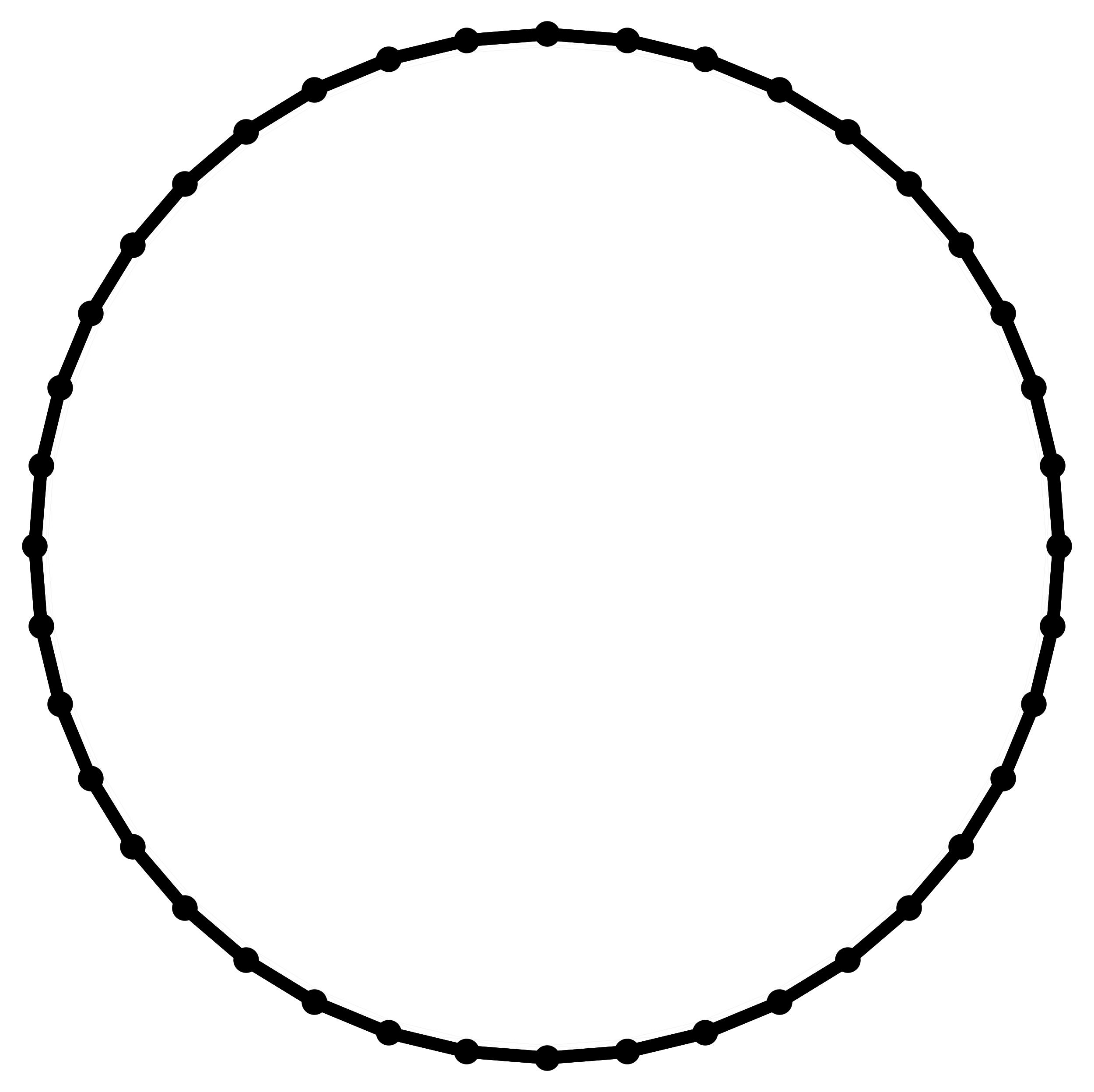
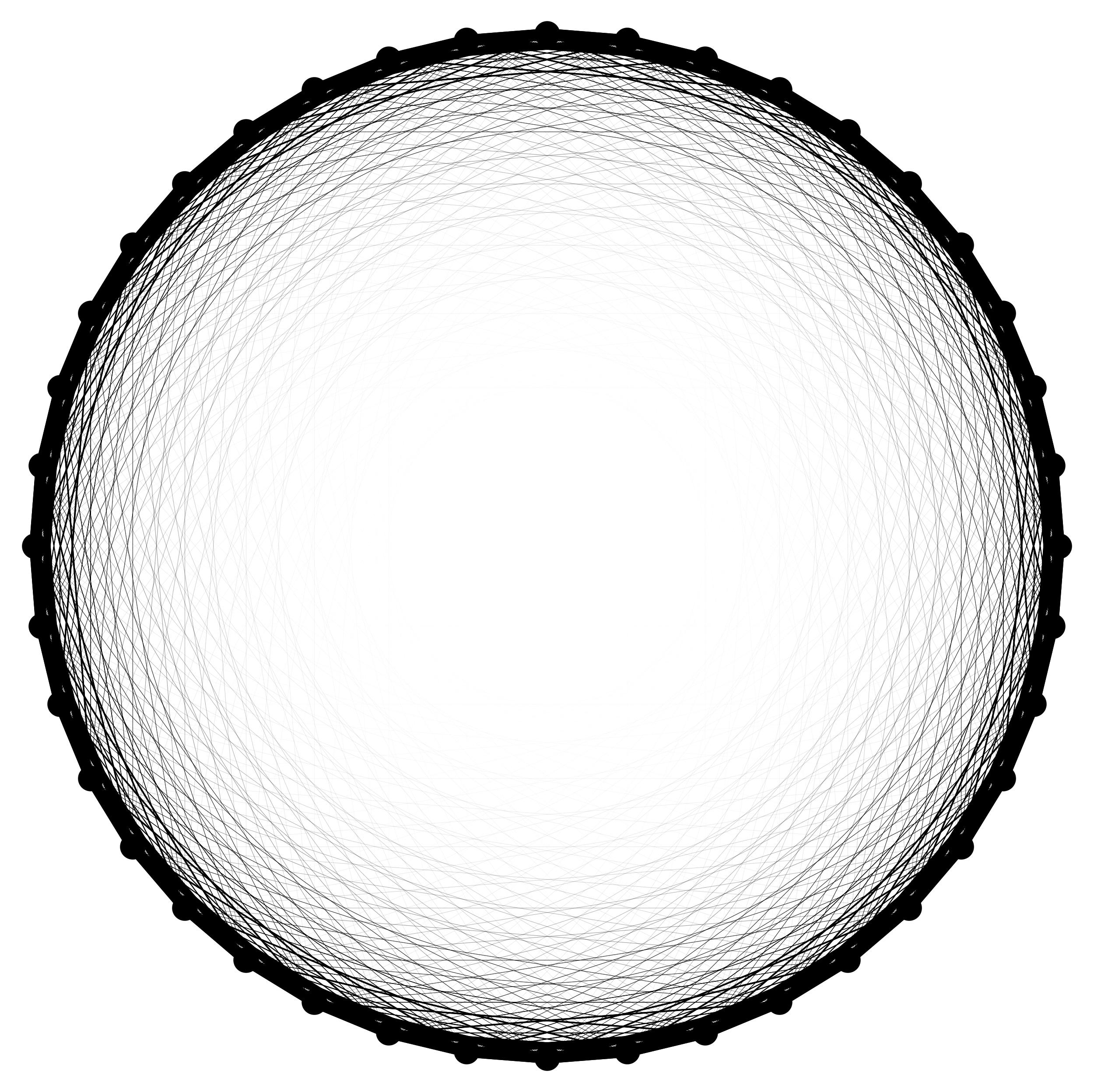
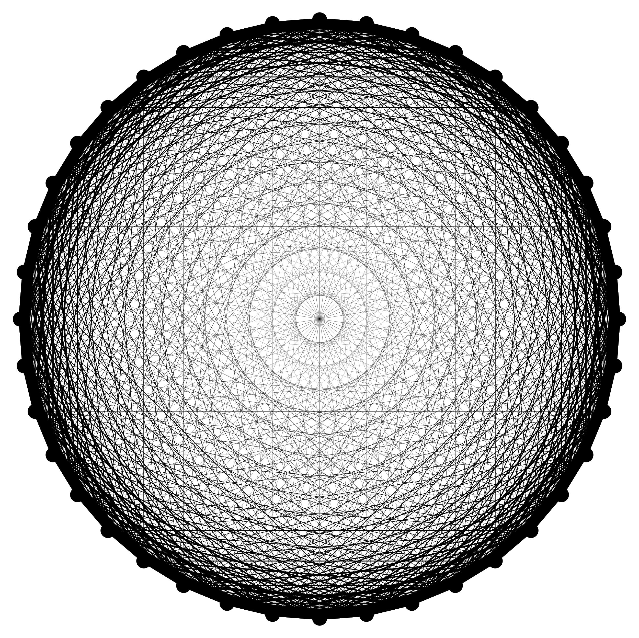
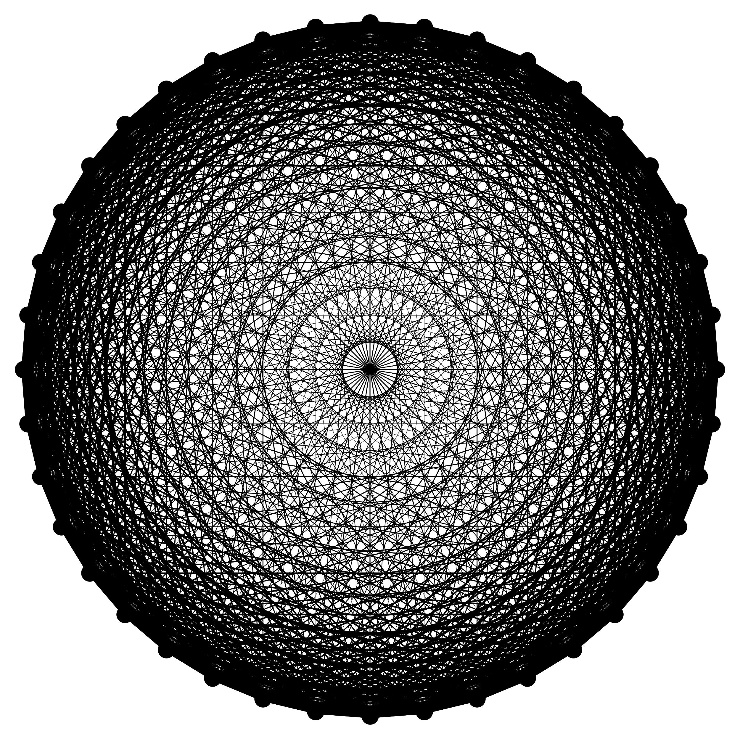
Figure 6: Snapshots of the graphs that arise from the numerical solution of $T_{ij}(t)$ at (a) $t=0$, (b) $t=15$, (c) $t=30$, (d) $t=45$ for $\epsilon=0.12$ with $R=U=\lambda=1$ and $L=40$. Dots represent sites, and the thickness of the line between sites $i$ and $j$ is proportional to $|T_{ij}|$.

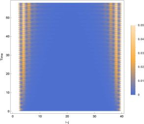
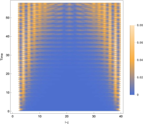
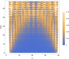
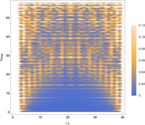
Figure 7: Density plot of $|T_{ij}(t)|$ shown as a function of $i-j$ and $t$ for (a) $\epsilon=0.08$, (b) $\epsilon=0.12$, (c) $\epsilon=0.16$, (d) $\epsilon=0.2$ with $R=U=\lambda=1$ and $L=40$.

In order to test the predictions of the perturbative analysis, we now solve Eq. (17) numerically for the initial condition in Eq. (19). In Fig. 6, the graphs that emerge from $T_{ij}(t)$ are shown at different time slices for $\epsilon=0.12$, where the thickness of the lines connecting sites are drawn in proportion to the magnitude of the bi-local field. At small $t$, sites are connected mainly through short-range bonds, maintaining the one-dimensional local structure. As time increases, the range of the bi-local fields grows, and all sites get connected to all other sites at late time. Fig. 7 shows the evolution of $T_{ij}(t)$ as a function of $i-j$ and $t$ for various choices of $\epsilon$. The translational symmetry of the initial condition guarantees that $T_{ij}(t)$ and $P_{ij}(t)$ depends on $i$ and $j$ only through $i-j$. Furthermore, $T_{ij}(t)=T_{iL+2i-j}(t)$ due to the periodic boundary condition. The profile of $P_{ij}(t)$ in the space of $i-j$ and $t$ is similar to that of $T_{ij}(t)$ shown in Fig. 7. As expected, the speed at which the range of the bi-local fields increases in real space strongly depends on $\epsilon$.

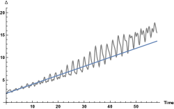
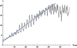
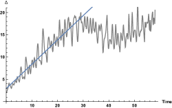
Figure 8: The range of the bi-local field defined in Eq. (33) plotted as a function of time for (a) $\epsilon=0.08$, (b) $\epsilon=0.12$, (c) $\epsilon=0.16$, (d) $\epsilon=0.2$ with $R=U=\lambda=1$ and $L=40$. The straight lines represent the best linear fits of $\Delta(t)$ in $0<t<30$.

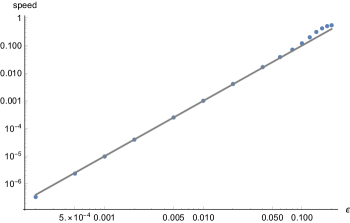
Figure 9: The rate at which $\Delta(t)$ increases in time obtained from a linear fit of $\Delta(t)$ in $0<t<30$ plotted in the log-log scale. The straight line is $10\epsilon^{2}$.

In order to quantify the speed of entanglement spread, we introduce

$$\Delta(t)\equiv 2\frac{\sum_{1\leq|i-j|\leq L/2}|T_{ij}(t)||i-j|}{\sum_{1\leq|i-j|\leq L/2}|T_{ij}(t)|}$$ (33)

which measures the range of the bi-local field in coordinate distance. Here the maximum size of the bi-local field is restricted to $|i-j|\leq L/2$ because of the periodic boundary condition. For the initial state with only short-range entanglement bonds, $\Delta(0)\sim O(1)$. In the other extreme limit, if $T_{ij}(t)$ spreads over the entire system and becomes independent of $i-j$, $\Delta(t)$ approaches $L/2$. In Fig. 8, we show the growth of $\Delta(t)$ for various values of $\epsilon$. At small $t$, $\Delta(t)$ increases linearly modulated by oscillatory contribution. The speed of the linear growth of $\Delta(t)$ at early time is plotted as a function of $\epsilon$ in Fig. 9. In the small $\epsilon$ limit, the speed scales with $\epsilon^{2}$, which is consistent with the perturbative analysis. This strong state dependence of the speed is contrasted to local Hamiltonians which typically exhibit an $O(1)$ dependence of speed on stateNajafi et al. (2018).

At larger $t$, the growth of $\Delta(t)$ exhibits an acceleration in time as is shown in Fig. 8. This non-linearity is more noticeable for small $\epsilon$ in which there is enough time before the range of the bi-local fields reach the system size. The acceleration can be attributed to the fact that further neighbor entanglement bonds can be created more easily once the state develops bonds beyond nearest neighbor sites in $t>0$. Eventually, $\Delta(t)$ stops growing once the range of the bi-local fields becomes comparable to the system size. In the late time limit, the bi-local field spreads over the entire system as is shown in Figs. 6 and 7. This implies that the state in the large $t$ limit supports entanglement entropy that scales with the coordinate volume of sub-systems. The time it takes for the system to reach such a state strongly depends on the amount of entanglement in the initial state.

State dependent coordinate speed can be understood as originating from state dependent geometry. It is noted that $\Delta(t)$ determines the range of hopping at time $t$ in Eq. (5). If we define the proper distance such that there exist hoppings only between sites within unit proper distance, sites which are separated by $\Delta(t)$ in coordinate distance are regarded to be within a unit proper distance. As $\Delta(t)$ increases in time, the proper size of the system decreases. In this sense, the time evolution shown in Fig. 7 can be viewed as a ‘collapsing universe’, where the proper size of the system shrinks in time .

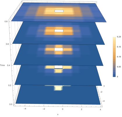
Figure 10: Density plot of $|T_{ij}(t)|$ shown as a function of $(x,y)$ at different time slices, where $x=x_{i}-x_{j}$, $y=y_{i}-y_{j}$ with $x_{i}=mod(i-1,\sqrt{L})+1$, $y_{i}=(i-x_{i})/\sqrt{L}+1$ for the initial condition in Eq. (34) with $\epsilon=0.2$, $R=U=\lambda=1$ and $L=100$. $|T_{ij}|\sim 0.5$ at $(x,y)=0$ is not shown in the density plot to increase the contrast for the non-onsite bi-local fields.

Next, we consider an example where the dimensionality of the emergent local theory is greater than one. For this, we consider an initial state which has a two-dimensional local structure,

$$T_{ij}(0) = T_{*}\delta_{ij}+\epsilon\delta_{d_{ij}^{(2)},1},$$

$$P_{ij}(0) = P_{*}\delta_{ij},$$ (34)

where $d_{ij}^{(2)}=\sqrt{\left[i-j\right]_{\sqrt{L}}^{2}+\left[\left\|\frac{i-1}{\sqrt{L}}\right\|-\left\|\frac{j-1}{\sqrt{L}}\right\|\right]_{\sqrt{L}}^{2}}$. In this case, there is no apparent locality for $T_{ij}(t)$ in terms of the one-dimensional coordinate $i$ and $j$. Instead, it exhibits a local structure associated with the two-dimensional lattice. Therefore we introduce a coordinate system $(x_{i},y_{i})$ which is related to site index $i$ via $x_{i}=mod(i-1,\sqrt{L})+1$, $y_{i}=(i-x_{i})/\sqrt{L}+1$. In Fig. 10, we show how the bi-local fields spread over the two-dimensional lattice as a function of time for the initial condition given by Eq. (34). Clearly the spread of entanglement follows the locality defined with respect to the two-dimensional lattice. This shows that the same Hamiltonian acts as a two-dimensional local Hamiltonian when applied to states that exhibit two-dimensional local structures, and as an one-dimensional Hamiltonian to states with one-dimensional local structures. In relatively local theories, topology, dimension and geometry are all emergent properties.

Figure 11: The range of the preformed bi-local fields (denoted as solid lines) determines the range of hopping for a local perturbation added to the system (denoted as dashed lines). For example, a local disturbance $\delta T_{ik}$ can hop to $\delta T_{ij}$ via the bonds that are formed between sites $k$ and $j$.

IV State dependent propagation of local disturbance

Now we examine how a local disturbance propagates in space. For this, we add an infinitesimally small local perturbation at $i=L/2$ to the initial state in Eq. (19) which supports the one-dimensional local structure,

$$T^{Q}_{ij}(0) = T_{*}\delta_{ij}+\epsilon\delta_{d_{ij}^{(1)},1}+Q\delta_{i,L/2}\delta_{j,L/2},$$

$$P^{Q}_{ij}(0) = P_{*}\delta_{ij},$$ (35)

where $Q$ denotes the strength of the local perturbation added at site $i=L/2$. In the limit that $Q\ll\epsilon$, the local perturbation propagates on top of the ‘geometry’ set by the bi-local fields formed in the absence of the local perturbation. We can express the solution in the presence of the local perturbation as

$$T^{Q}_{ij}(t) = T_{ij}(t)+\delta T_{ij}(t),$$

$$P^{Q}_{ij}(t) = P_{ij}(t)+\delta P_{ij}(t),$$ (36)

where $T_{ij}(t),P_{ij}(t)$ are the solution of the equation of motion with $Q=0$, and $\delta T_{ij}(t),\delta P_{ij}(t)\sim Q$ represent the deviation generated from the local perturbation. To the leading order in $Q$, $\delta T_{ij}(t),\delta P_{ij}(t)$ satisfy,

$$-i~{}\partial_{\tau}\delta T_{ij} = R\left(-2\delta T_{ij}+8\delta T_{ik}P_{kl}T_{lj}+8T_{ik}\delta P_{kl}T_{lj}+8T_{ik}P_{kl}\delta T_{lj}\right)$$

$$-4U\left(\delta T_{ik}T_{kj}+T_{ik}\delta T_{kj}\right)+2\lambda\delta P_{ii}\delta_{ij},$$

$$i~{}\partial_{\tau}\delta P_{ij} = R\left(-2\delta P_{ij}+8\delta P_{ik}T_{kl}P_{lj}+8P_{ik}\delta T_{kl}P_{lj}+8P_{ik}T_{kl}\delta P_{lj}\right)$$ (37)

$$-4U\left(\delta P_{ik}T_{kj}+P_{ik}\delta T_{kj}+\delta T_{ik}P_{kj}+T_{ik}\delta P_{kj}\right).$$

Here the bi-local fields that are already formed in the absence of the local perturbation sets the background on which the perturbation propagates. The range of the hopping for the perturbation is set by the range of the preformed bi-local fields. For example, $-i~{}\partial_{\tau}\delta T_{ij}\sim R\delta T_{ik}P_{kl}T_{lj}$ in Eq. (37) describes the processes in which $\delta T_{ik}$ defined on link $(i,k)$ jumps to link $(i,j)$ via $P_{kl}T_{lj}$ that provides a connection between $k$ and $j$. If $P_{kl}T_{lj}\sim e^{-d^{(1)}_{kj}/\xi}$, $\delta T_{ik}$ jumps by coordinate distance $\xi$ at a time. This is illustrated in Fig. 11. Since the profiles of $T_{ij}$ and $P_{ij}$ strongly depend on the initial state, so does the coordinate speed at which local disturbance propagates in space. As time increases, the range of $T_{ij}$ and $P_{ij}$ increases. Accordingly, we expect that the coordinate speed for the propagation of the local disturbance increases in time.

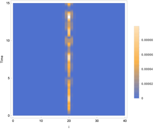
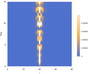
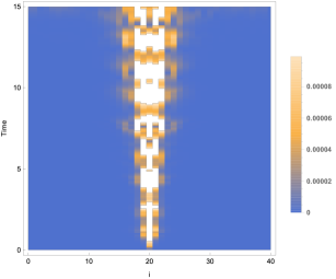
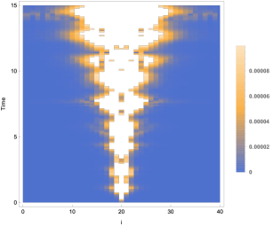
Figure 12: The relative local energy density $\Delta h_{i}(t)$ plotted in the space of $i$ and $t$ for the initial condition in Eq. (35) with $R=U=\lambda=1$, $Q=10^{-3}$ and $L=40$ for (a) $\epsilon=0.08$, (b) $\epsilon=0.12$, (c) $\epsilon=0.16$ and (b) $\epsilon=0.2$.

We check this through the numerical solution obtained for the initial condition in Eq. (35). To keep track of how the local perturbation propagate in space, we introduce

$$h_{i} = R\left(-2T_{ii}P_{ii}+4(T_{ii}P_{ii})^{2}\right)+U\left(2T_{ii}-4T_{ii}^{2}P_{ii}\right)+\lambda P_{ii}^{2},$$ (38)

where the index $i$ is not summed over. This corresponds to the conserved energy density for the direct product state. For general states, this is neither conserved nor real. Nonetheless, this is a useful measure that characterizes how far each site is driven away from the ultra-local fixed point. In Fig. 12, we plot

$$\Delta h_{i}(t)=\left|\frac{h_{i}(t)-h_{L}(t)}{h_{L}(t)}\right|$$ (39)

as a function of $i$ and $t$. $\Delta h_{i}(t)$ measures the deviation of the ‘local energy density’ at site $i$ relative to the local energy density at a site far away from the site with the local perturbation. As is shown in Fig. 12, the speed at which the local disturbance propagates in space strongly depends on $\epsilon$. The coordinate speed of the propagation increases with time as well. This is due to the fact that the perturbation can hop by larger coordinate distances using larger entanglement bonds at later time. In other words, the shrinking universe makes coordinate speed of propagation to increase. The acceleration of the propagating mode in coordinate speed is more manifest for large $\epsilon$ as is shown in Fig. 12 (d). For small $\epsilon$, it is hard to differentiate the speed of the propagating mode from the speed of entanglement spread because both are small.

It is emphasized that $\epsilon$ is not a parameter of the Hamiltonian, but a parameter that characterizes the amount of entanglement in states. The state dependent speeds of entanglement spread and wave propagation is a hallmark of relatively local Hamiltonians. The state dependence of coordinate speed can be understood in terms of state dependent geometry with a fixed proper speed. A state which is close to a direct product state gives rise to a geometry whose proper size is large. This translates to a small speed of propagation when the speed is measured in coordinate distance. Conversely, a state with a larger entanglement has a geometry with shorter proper distance, and exhibits a larger coordinate speed. Relatively local Hamiltonians do not satisfy a bound on how fast entanglement can spread in terms of coordinate speedLieb and Robinson (1972). However, it is likely that there exists a bound on a proper speed, where the physical distance is measured with respect to state dependent geometry in the large $N$ limit.

V Summary

In this paper, we construct a simple relatively local Hamiltonian for $N$ scalar fields. The Hamiltonian is defined on a set of sites which has no preferred background. Although the Hamiltonian is non-local as a quantum operator, it acts as a local Hamiltonian in the large $N$ limit when applied to states whose pattern of entanglement exhibits a local structure. The dimension, topology and geometry of the emergent local theory are determined by states. This is shown by examining how states with local structures evolve under the time evolution generated by the relatively local Hamiltonian. The fact that geometry is determined by state manifests itself as state-dependent coordinate speeds at which entanglement and local perturbation spread. The state-dependent coordinate speed is naturally understood as originating from the state dependent metric. The metric associated with a saddle-point configuration can be explicitly determined from the equation of motion that small fluctuations of the collective variables obey in the continuum limit if the analytic form of the saddle-point solution is knownLee (2016). In the present case, the analytic solution for the strongly time-dependent saddle-point solution is not yet available, and we postpone the derivation of the metric to future work. The metric determined in this manner is expected to satisfy the condition that gapless modes propagate with a fixed proper speed.

Generically, states with local structures undergo ‘big crunches’ in which locality is destroyed as sites become globally connected at a later time. One can also consider a ‘big bang’ where locality emerges out of initial states that do not have local structure. The time reversal symmetry guarantees that there exists a set of states that exhibit such dynamically emergent locality at least over a finite window of time. Namely, the backward evolution of the big crunches, whose evolution is governed by the same Hamiltonian due to the time reversal symmetry, describes an expanding universe where the proper volume of the system increases as states become less entangled in time. It would be of great interest to understand how generic such states are in the Hilbert space.

VI A possible roadmap toward quantum gravity

In relatively local theories, the metric is nothing but a collective variable that determines the pattern of entanglement of underlying quantum matter. The relatively local theory is a background independent theory of geometry because geometry is dynamically determined and there is no fixed background metric. In this section, we discuss other aspects of gravity that need to be incorporated into a relatively local theory so that it becomes a full quantum theory of gravity that has a chance to reproduce the general relativity in the semi-classical limit.

The key additional ingredient is the diffeomorphism invariance. The present theory has the discrete spatial diffeomorphism. However, it does not have the full spacetime diffeomorphism invariance because it has a preferred time. In the Hamiltonian formulation of Einstein’s general relativity, spacetime diffeomorphism is represented as the algebra obeyed by the three momentum and one Hamiltonian densities. It is likely that not all details of the algebra derived from the classical general relativity can be carried over to the quantum level. The precise form of the constraint algebra remains unknown at the quantum level because of the difficulty in regularizing UV divergences of local operators in the general relativity. More importantly, the algebra for the four-dimensional spacetime should be viewed only as an approximation of a more general algebra if the dimension is an emergent property as is the case for relatively local theories. Nonetheless, the gauge principle itself is likely to survive at the quantum level. If so, there should exists a closed algebra of constraints that reduce to diffeomorphisms of manifolds in states with local structures.

In theories where metric emerges as a collective degree freedom, the underlying quantum matter provides an unambiguous norm in the Hilbert space. This may give new insights into the problem of time in quantum gravity. In principle, physical states should be invariant under all gauge transformations generated by the constraints. However, states that are invariant under the constraints are generally non-normalizable, and physical states with finite norms spontaneously break the symmetry generated by the constraints. In this framework, a non-trivial time evolution in quantum gravity can be viewed as a consequence of the spontaneously broken gauge symmetryLee (2018).

The full theory of collective variables also includes other dynamical fields besides metric. For example, the bi-local field considered in this paper can be decomposed into an infinite tower of local fields with higher spins. They should contribute to the energy-momentum tensor that source the curvature for the spin $2$ mode. The way metric is coupled with other fields is dictated by the constraint algebra. At the microscopic level, such interactions describe couplings among different collective modes of the same underlying matter. For example, the spin $2$ collective mode that dictates the entanglement of the matter can be affected by the spin $0$ collective mode which describes disturbances localized at sites.

In the tower of modes with general spins, there exist gauge fields if there is a symmetry under which the collective variables carry non-trivial charges. For example, Eq. (2) is invariant under the site-dependent $Z_{2}$ symmetry,

$$\phi^{a}_{i} \rightarrow (-1)^{\delta_{ij}}\phi^{a}_{i},$$

$$T_{i_{1}i_{2}..i_{2n}} \rightarrow (-1)^{\sum_{k=1}^{2n}\delta_{i_{k}j}}T_{i_{1}i_{2}..i_{2n}}$$ (40)

for each $j$, and so is Eq. (5). As a consequence, Eqs. (15) and (16) take the form of the $Z_{2}$ gauge theory in the temporal gauge, where the sign of the bi-local field $T_{ij}$ becomes the dynamical $Z_{2}$ gauge field. In background independent theories, the emergence of gauge fields is general beyond the specific group and the one-form gauge field. For example, in the presence of unbreakable closed loops, a dynamical two-form U(1) gauge field arises in the bulkLee (2012). This is similar to the way in which global symmetries are promoted to gauge symmetries in the quantum renormalization groupNAKAYAMA (2013).

Finally, we comment on the relation with other models of emergent locality. In Refs. Konopka et al. (2006, 2008), models of dynamical graph have been considered where a graph with locality emerges as a ground state. The main feature that is shared by the models of quantum graphity and the present model is that both theories are background independent. Only a special set of states exhibit locality. The dimension, topology and geometry are dynamical properties of those states that have locality. There are also some important differences. The first difference lies in the fundamental degree of freedom. In the graph model, dynamical degrees of freedom are assigned to every possible link between vertices. Different graphs are formed depending on which links are turned on or off. In the present theory, on the other hand, entanglement between matter fields determine the geometry. While connectivity itself is the fundamental degree of freedom in the graph model, collective variables for underlying local degrees of freedom replaces the role of links in the present model. In that the fundamental degrees of freedom are ordinary matter fields, the present approach is more closely related to the way gravity emerges from field theories in AdS/CFT correspondenceMaldacena (1999); Witten (1998); Gubser et al. (1998). The fact that metric is a collective variable of quantum matter in the present model gives rise to a second important distinction from other models. In the graph models, each vertex can be in principle connected to any number of vertices, and one needs to introduce an energetic penalty to suppress graphs with too many connections. In the present model, on the other hand, there is a limited amount of dynamical connections a site can form with other sites due to the monogamous nature of entanglement. While this is not manifest in the large $N$ limit with a small number of sites ($L$), this constraint is expected to play an important role in dynamically suppressing non-local graphs in the physical limit with $L\gg N$. The third difference is the locality of the effective theory that emerges once a local structure is dynamically selected. In the present model, the effective theory that describes small fluctuations around a saddle-point with local structure is a local theory as is shown in Sec. IV. This seems less clear in the graph models. The emergence of a local graph does not necessarily guarantee the locality of the effective theory that describes small fluctuations of graph because the underlying Hamiltonian that selects a local graph is highly non-local.

Appendix A Method of numerical integration

In order to solve Eq. (17) numerically, we employ the symplectic integrator developed for non-separable Hamiltonian systemsTao (2016). Eq. (17) is not separable, and the usual symplectic integrator can not be readily applied. Therefore, we first double the degrees of freedom and introduce a Hamiltonian for the enlarged system,

$${\cal H}_{t}[T_{A},P_{A},T_{B},P_{B}] = {\cal H}[T_{A},P_{B}]+{\cal H}[T_{B},P_{A}]+\frac{\omega}{2}\sum_{ij}\left[(P_{A;ij}-P_{B,ij})^{2}-(T_{A;ij}-T_{B,ij})^{2}\right].$$

We solve the equation of motion for the enlarged system with the initial condition, $T_{A;ij}(0)=T_{B;ij}(0)=\bar{T}_{ij}$ and $P_{A;ij}(0)=P_{B;ij}(0)=\bar{P}_{ij}$. The exact solution to the enlarged equation of motion agrees with the solution to Eq. (17). The numerical advantage of using Eq. (LABEL:Ht) is that one can implement the symplectic algorithm that prevents total energy from drifting as a result of accumulated numerical error. We implement an evolution of a state from $t$ to $t+dt$ as

$$\left(\begin{array}[]{c}T_{A;ij}(t+dt)\\ P_{A;ij}(t+dt)\\ T_{B;ij}(t+dt)\\ P_{B;ij}(t+dt)\end{array}\right) = \phi^{dt/2}_{1}\circ\phi^{dt/2}_{2}\circ\phi^{dt}_{3}\circ\phi^{dt/2}_{2}\circ\phi^{dt/2}_{1}\left(\begin{array}[]{c}T_{A;ij}(t)\\ P_{A;ij}(t)\\ T_{B;ij}(t)\\ P_{B;ij}(t)\end{array}\right),$$ (50)

where

$$\phi^{\delta}_{1}\left(\begin{array}[]{c}T_{A;ij}\\ P_{A;ij}\\ T_{B;ij}\\ P_{B;ij}\end{array}\right) = \left(\begin{array}[]{c}T_{A;ij}\\ P_{A;ij}-i\delta\frac{\partial{\cal H}[T_{A},P_{B}]}{\partial T_{A;ij}}\\ T_{B;ij}+i\delta\frac{\partial{\cal H}[T_{A},P_{B}]}{\partial P_{B;ij}}\\ P_{B;ij}\end{array}\right),~{}~{}~{}~{}~{}~{}~{}\phi^{\delta}_{2}\left(\begin{array}[]{c}T_{A;ij}\\ P_{A;ij}\\ T_{B;ij}\\ P_{B;ij}\end{array}\right)=\left(\begin{array}[]{c}T_{A;ij}+i\delta\frac{\partial{\cal H}[T_{B},P_{A}]}{\partial P_{A;ij}}\\ P_{A;ij}\\ T_{B;ij}\\ P_{B;ij}-i\delta\frac{\partial{\cal H}[T_{B},P_{A}]}{\partial T_{B;ij}}\end{array}\right),$$ (67)

$$\phi^{\delta}_{3}\left(\begin{array}[]{c}T_{A;ij}\\ P_{A;ij}\\ T_{B;ij}\\ P_{B;ij}\end{array}\right) = \frac{1}{2}\left(\begin{array}[]{c}T_{A;ij}+T_{B;ij}+\cos(2\omega\delta)(T_{A;ij}-T_{B;ij})+i\sin(2\omega\delta)(P_{A;ij}-P_{B;ij})\\ P_{A;ij}+P_{B;ij}+i\sin(2\omega\delta)(T_{A;ij}-T_{B;ij})+\cos(2\omega\delta)(P_{A;ij}-P_{B;ij})\\ T_{A;ij}+T_{B;ij}-\cos(2\omega\delta)(T_{A;ij}-T_{B;ij})-i\sin(2\omega\delta)(P_{A;ij}-P_{B;ij})\\ P_{A;ij}+P_{B;ij}-i\sin(2\omega\delta)(T_{A;ij}-T_{B;ij})-\cos(2\omega\delta)(P_{A;ij}-P_{B;ij})\end{array}\right).$$ (76)

The symplectic form $dT_{A;ij}\wedge dP_{A;ij}+dT_{B;ij}\wedge dP_{B;ij}$ is preserved under Eq. (50). In this paper, we use $R=U=\lambda=1$, $\omega=10$ and $dt=10^{-3}$.

References

- Wichmann and Crichton (1963) E. H. Wichmann and J. H. Crichton, Phys. Rev. 132, 2788 (1963), URL https://link.aps.org/doi/10.1103/PhysRev.132.2788.
- Marolf (2015) D. Marolf, Phys. Rev. Lett. 114, 031104 (2015), URL https://link.aps.org/doi/10.1103/PhysRevLett.114.031104.
- Lee (2018) S.-S. Lee, Journal of High Energy Physics 2018, 43 (2018), ISSN 1029-8479, URL https://doi.org/10.1007/JHEP10(2018)043.
- Sachdev and Ye (1993) S. Sachdev and J. Ye, Phys. Rev. Lett. 70, 3339 (1993), URL https://link.aps.org/doi/10.1103/PhysRevLett.70.3339.
- Kitaev (2015) A. Kitaev, KITP strings seminar and Entanglement (2015), URL http://online.kitp.ucsb.edu/online/entangled15/.
- Ryu and Takayanagi (2006) S. Ryu and T. Takayanagi, Phys. Rev. Lett. 96, 181602 (2006), URL http://link.aps.org/doi/10.1103/PhysRevLett.96.181602.
- Hubeny et al. (2007) V. E. Hubeny, M. Rangamani, and T. Takayanagi, Journal of High Energy Physics 2007, 062 (2007), URL http://stacks.iop.org/1126-6708/2007/i=07/a=062.
- Van Raamsdonk (2010) M. Van Raamsdonk, Gen. Rel. Grav. 42, 2323 (2010), [Int. J. Mod. Phys.D19,2429(2010)], eprint 1005.3035.
- Casini et al. (2011) H. Casini, M. Huerta, and R. C. Myers, Journal of High Energy Physics 2011, 1 (2011), ISSN 1029-8479, URL http://dx.doi.org/10.1007/JHEP05(2011)036.
- Lewkowycz and Maldacena (2013) A. Lewkowycz and J. Maldacena, Journal of High Energy Physics 2013, 1 (2013), ISSN 1029-8479, URL http://dx.doi.org/10.1007/JHEP08(2013)090.
- Maldacena (1999) J. M. Maldacena, Int.J.Theor.Phys. 38, 1113 (1999), eprint hep-th/9711200.
- Witten (1998) E. Witten, Adv.Theor.Math.Phys. 2, 253 (1998), eprint hep-th/9802150.
- Gubser et al. (1998) S. Gubser, I. R. Klebanov, and A. M. Polyakov, Phys.Lett. B428, 105 (1998), eprint hep-th/9802109.
- Maldacena and Susskind (2013) J. Maldacena and L. Susskind, Fortschritte der Physik 61, 781 (2013), eprint https://onlinelibrary.wiley.com/doi/pdf/10.1002/prop.201300020, URL https://onlinelibrary.wiley.com/doi/abs/10.1002/prop.201300020.
- Lee (2016) S.-S. Lee, Journal of High Energy Physics 2016, 44 (2016), ISSN 1029-8479, URL https://doi.org/10.1007/JHEP09(2016)044.
- Cao et al. (2017) C. Cao, S. M. Carroll, and S. Michalakis, Phys. Rev. D 95, 024031 (2017), URL https://link.aps.org/doi/10.1103/PhysRevD.95.024031.
- Bus (1996) The Quantum Theory of Measurement (Springer Berlin Heidelberg, Berlin, Heidelberg, 1996), pp. 25–90, ISBN 978-3-540-37205-9, URL https://doi.org/10.1007/978-3-540-37205-9_3.
- Bender et al. (1999) C. M. Bender, S. Boettcher, and P. N. Meisinger, Journal of Mathematical Physics 40, 2201 (1999), eprint https://doi.org/10.1063/1.532860, URL https://doi.org/10.1063/1.532860.
- Nozaki et al. (2013) M. Nozaki, T. Numasawa, and T. Takayanagi, Journal of High Energy Physics 2013, 80 (2013), ISSN 1029-8479, URL https://doi.org/10.1007/JHEP05(2013)080.
- Jurcevic et al. (2014) P. Jurcevic, B. P. Lanyon, P. Hauke, C. Hempel, P. Zoller, R. Blatt, and C. F. Roos, Nature 511, 202 EP (2014), URL http://dx.doi.org/10.1038/nature13461.
- Rangamani et al. (2016) M. Rangamani, M. Rozali, and A. Vincart-Emard, Journal of High Energy Physics 2016, 69 (2016), ISSN 1029-8479, URL https://doi.org/10.1007/JHEP04(2016)069.
- Casini et al. (2016) H. Casini, H. Liu, and M. Mezei, Journal of High Energy Physics 2016, 77 (2016), ISSN 1029-8479, URL https://doi.org/10.1007/JHEP07(2016)077.
- Liu and Suh (2014) H. Liu and S. J. Suh, Phys. Rev. Lett. 112, 011601 (2014), URL https://link.aps.org/doi/10.1103/PhysRevLett.112.011601.
- Mezei and Stanford (2017) M. Mezei and D. Stanford, Journal of High Energy Physics 2017, 65 (2017), ISSN 1029-8479, URL https://doi.org/10.1007/JHEP05(2017)065.
- Kundu and Pedraza (2017) S. Kundu and J. F. Pedraza, Phys. Rev. D 95, 086008 (2017), URL https://link.aps.org/doi/10.1103/PhysRevD.95.086008.
- Najafi et al. (2018) K. Najafi, M. A. Rajabpour, and J. Viti, Phys. Rev. B 97, 205103 (2018), URL https://link.aps.org/doi/10.1103/PhysRevB.97.205103.
- Lieb and Robinson (1972) E. H. Lieb and D. W. Robinson, Communications in Mathematical Physics 28, 251 (1972), ISSN 1432-0916, URL https://doi.org/10.1007/BF01645779.
- Lee (2012) S.-S. Lee, Nucl.Phys. B862, 781 (2012), eprint 1108.2253.
- NAKAYAMA (2013) Y. NAKAYAMA, International Journal of Modern Physics A 28, 1350166 (2013), eprint https://doi.org/10.1142/S0217751X13501662, URL https://doi.org/10.1142/S0217751X13501662.
- Konopka et al. (2006) T. Konopka, F. Markopoulou, and L. Smolin, arXiv e-prints hep-th/0611197 (2006), eprint hep-th/0611197.
- Konopka et al. (2008) T. Konopka, F. Markopoulou, and S. Severini, Phys. Rev. D 77, 104029 (2008), URL https://link.aps.org/doi/10.1103/PhysRevD.77.104029.
- Mozaffar and Mollabashi (2016) M. R. M. Mozaffar and A. Mollabashi, Journal of High Energy Physics 2016, 15 (2016), ISSN 1029-8479, URL https://doi.org/10.1007/JHEP03(2016)015.
- Tao (2016) M. Tao, Phys. Rev. E 94, 043303 (2016), URL https://link.aps.org/doi/10.1103/PhysRevE.94.043303.