Robust Tests for Treatment Effect in Survival Analysis under Covariate-Adaptive Randomization

Abstract

Covariate-adaptive randomization is popular in clinical trials with sequentially arrived patients for balancing treatment assignments across prognostic factors which may have influence on the response. However, existing theory on tests for treatment effect under covariate-adaptive randomization is limited to tests under linear or generalized linear models, although covariate-adaptive randomization has been used in survival analysis for a long time and its main application is in survival analysis. Often times, practitioners would simply adopt a conventional test such as the log-rank test or score test to compare two treatments, which is controversial since tests derived under simple randomization may not be valid under other randomization schemes. In this article, we prove that the log-rank test valid under simple randomization is conservative in terms of type I error under covariate-adaptive randomization, and the robust score test developed under simple randomization is no longer robust under covariate-adaptive randomization. We then propose a calibration type log-rank or score test that is valid and robust under both simple randomization and a large family of covariate-adaptive randomization schemes. Furthermore, we obtain Pitman’s efficacy of log-rank and score tests to compare their asymptotic relative efficiency. Simulation studies about the type I error and power of various tests are presented under several popular randomization schemes.

1 Introduction

In a clinical trial to compare the effectiveness of two treatments, simple randomization, also known as complete randomization, assigns patients independently into two treatment groups with equal probability. Simple randomization is widely accepted because it provides a basis for statistical inference. In survival analysis, however, patients are not all available for simultaneous assignment of treatment but rather arrive sequentially and must be treated immediately. In such a case, simple randomization may yield highly disparate sample sizes between treatment arms across prognostic factors, e.g., institution, disease stage, prior treatment, sex, and age, which are known or thought to have significant influence on the response. Imbalance of treatment assignments across these factors may cause a confounding of the treatment effect and obscure the causation of active treatment itself to the observed effect.

Many covariate-adaptive randomized treatment allocation schemes have been proposed, which have advantages of minimizing imbalance between treatment groups across covariates or prognostic factors, reducing selection bias, minimizing accidental bias, and improving efficiency in inference (Efron, 1971; Pocock and Simon, 1975; Wei, 1977, 1978a, 1978b; Weir and Lees, 2003). One of the oldest covariate-adaptive randomization methods is the minimization procedure developed by Taves (1974). Pocock and Simon (1975) generalized Taves’ method and proposed to sequentially allocate patients with different probabilities to ensure treatment arms are marginally balanced within levels of each prognostic factor. A special case of Pocock and Simon’s method is to apply the biased coin method (Efron, 1971) to patients stratified by prognostic factors, which is referred to as the covariate-adaptive biased coin method. Another popular method that has been extensively implemented in clinical studies is the permuted block design stratified based on prognostic covariates (Zelen, 1974). A nice summary of the randomization schemes can be found in Schulz and Grimes (2002). As pointed out in Taves (2010), there are over 500 clinical trials which implemented Pocock and Simon’s procedure to balance important covariates from 1989 to 2008. More recent examples of applying covariate-adaptive randomization can be found in van der Ploeg et al. (2010), Fakhry et al. (2015), Breugom et al. (2015), Stott et al. (2017), and Sun et al. (2018). The applications of covariate-adaptive randomization are not limited to clinical trials, and they are particularly relevant for randomized experiments with many interventions, for example, in mobile health.

In spite of the high prevalence of covariate-adaptive randomization, conventional tests are often utilized in practice (e.g., in 2018 New England Journal of Medicine, there are 9 articles using stratified permuted block design but conventional log-rank test or Wald’s test), which has been raising concerns because statistical testing of the treatment effect should be performed using a test procedure valid under the particular randomization scheme used in data collection. Here, the validity of a test procedure refers to the type I error rate of the test is no larger than a given significance level, at least in the limiting sense. Shao et al. (2010) initiated theoretical investigations on the validity of two sample $t$-test under covariate-adaptive biased coin randomization when the response follows a linear model. More results based on $t$-test under linear or generalized linear models and other covariate-adaptive randomization methods are given by Shao and Yu (2013), Ma et al. (2015) and Bugni et al. (2017). However, so far the study of testing hypotheses under covariate-adaptive randomization in survival analysis is limited to empirical investigations, despite the fact that covariate-adaptive randomization has been used in survival analysis for a long time, and its main application is in survival analysis. The main reason for lack of theoretical results is that tests commonly used in survival analysis, such as the log-rank and score tests are highly non-linear, thus are more complicated to study than tests used under additive models. Moreover, censoring adds another layer of complexity. In this article, we will highlight the commonalities and differences between our results and the results derived under additive models.

To obtain a valid test, one approach is to construct a test under a correctly specified model that includes all covariates used in covariate-adaptive randomization (Shao et al., 2010). However, it is not always practical to include all covariates in the model for constructing a valid test procedure, mainly because it is difficult to incorporate some covariates in a model and the more covariates are included, the more likely the model may be misspecified or too complicated to be useful. For example, as described in Breugom et al. (2015), a Cox proportional hazard model was adopted for survival data under a permuted block randomization of size six with stratification according to center, residual tumor, time between last irradiation and surgery, and preoperative treatment. It is difficult to specify a correct Cox model with these many covariates.

Thus, it is of great interest to derive tests that are valid under covariate-adaptive randomization and robust against any model misspecification, either some or all covariates used in randomization are not included in the Cox model, or the proportional hazard is completely wrong. The robustness against misspecification of Cox proportional hazard model has been studied in survival analysis (Lin and Wei, 1989; Kong and Slud, 1997; DiRienzo and Lagakos, 2002), but all results are limited to simple randomization.

The purpose of our research is to establish a comprehensive theory for log-rank, score, or Wald’s test of treatment effect in survival analysis under covariate-adaptive randomization. Our major contributions are three folds. First, we initiate the studies beyond tests under additive models, where we develop novel technical tools to address the non-linear nature of tests in survival analysis. Second, the robust hypothesis testing results in survival analysis are generalized from simple randomization to a large family of covariate-adaptive randomization, where data are dependent. Third, we fill in the gap between theory and practice and provide some guidance in this field where covariate-adaptive randomization has its major application.

After a detailed description of some popular covariate-adaptive randomization methods, in Section 2 we define the validity and conservativeness of tests, and the robustness. Section 3 presents asymptotic results of the score test under covariate-adaptive randomization, which leads to results on the validity and conservativeness of score test. This theory also covers the popular log-rank test. Since the score test and log-rank test are conservative under covariate-adaptive randomization, we propose a calibration method to construct valid tests which are also robust against model misspecification. To compare powers of tests, results on Pitman’s asymptotic relative efficiency are also included. In Section 4, simulation studies are conducted to examine the finite sample performances of tests and our theory regarding type I error and power is supported by simulation results. Section 5 summarizes our main findings. All technical details are given in the Appendix in Supplemental Material.

2 Design and Hypothesis Testing

2.1 Design

Let $n$ be the total number of patients in both arms, $\bm{V}_{i}$ be a vector of all measured and unmeasured covariates for the $i$th patient, which can be time-varying but the index $t$ is omitted, $\bm{Z}_{i}$ be a subset of $\bm{V}_{i}$, a discrete time-independent baseline measured covariate with finitely many categories for which we want to balance by covariate-adaptive randomization, and $I_{i}$ be the treatment indicator equaling $j$ if patient $i$ is assigned to treatment $j$, $j=0,1$.

We first consider the design, i.e., the method of generating treatment assignments, $I_{i}$’s. Treatment assignments under simple randomization are achieved by tossing a fair coin independently with the other variables so that $P(I_{i}=1)=P(I_{i}=0)=1/2$ for all $i$. To alleviate the imbalance between treatment groups, permuted block randomization is most frequently used, which can ensure the balancedness of two treatment groups at the end of every block. For example, with a block of $2b$ consecutively enrolled patients, exactly $b$ patients are randomly allocated to one treatment. The block size $2b$ can remain fixed throughout the trial or varied under a pre-specified pattern. The permuted block randomization is very easy to implement and is quite effective in eliminating unbalanced design, but sometimes it is criticized to be too deterministic to result in selection bias. Biased coin (Efron, 1971) is an alternative approach that can assure the imbalance to be controlled in probability without enforcing strict balancing. It assigns the $(k+1)$th patient according to

$$P(I_{k+1}=1)=\left\{\begin{array}[]{lc}p,&D_{k}<0\\ 1/2,&D_{k}=0\\ 1-p,&D_{k}>0\end{array},\right.$$ (1)

where $p$ is a prefixed probability greater than $1/2$, $D_{0}=0$ and $D_{k}=\sum_{i=1}^{k}(2I_{i}-1)$, the difference between the number of patients in treatment 1 and treatment 0 after $k$ assignments have been made. The urn design (Wei, 1977, 1978a, 1978b) belongs to the family of biased coin randomization with adaptively changing $p$. It assigns the $(k+1)$th patient according to (1) but with $p$ being $p_{k}=\frac{1}{2}+\frac{\omega|D_{k}|}{2(2s+\omega k)}$, where $\omega,s$ are pre-specified non-negative real numbers. When $\omega=0$, it is the same as the simple randomization. Note that $p_{k}$ tends toward $\frac{1}{2}$ as $k$ increases with fixed $D_{k}$, indicating the urn design would force balancedness at the beginning of the treatment allocation, and approach simple randomization as the size of the trial increases.

The aforementioned three adaptive randomizations are not themselves covariate adaptive since they do not use any covariate information in treatment allocation. To balance across patients’ prognostic profile, we could form strata by levels of $\bm{Z}_{i}$ and apply these randomization methods within each stratum. They are named stratified permuted block randomization, covariate-adaptive biased coin randomization, and stratified urn design, respectively.

To characterize the property of covariate-adaptive randomization, we define the within strata imbalance as follows,

$$D_{n}(\bm{z})=\sum_{i:\bm{Z}_{i}=\bm{z}}(2I_{i}-1)=\sum_{i:\bm{Z}_{i}=\bm{z}}I_{i}-\sum_{i:\bm{Z}_{i}=\bm{z}}(1-I_{i}).$$ (2)

The first simple property is

(D1) $n_{\bm{z}}^{-1/2}D_{n}(\bm{z})=o_{p}(1)$ for every $\bm{z}$, where $n_{\bm{z}}$ is the number of subjects with $\bm{Z}_{i}=\bm{z}$.

Stratified permuted block randomization and covariate-adaptive biased coin randomization are examples of covariate-adaptive randomization satisfying (D1). Specifically, under stratified permuted block randomization, for every $\bm{z}$, $D_{n}(\bm{z})$ is at maximum half of block size if the block size is fixed, or half of the last block size if the block size varies; thus $D_{n}(\bm{z})$ is bounded. As for covariate-adaptive biased coin randomization, it is proved in Efron (1971) that $D_{n}(\bm{z})$ is bounded in probability for every $\bm{z}$. Another type of covariate adaptive randomization designs has the property

(D2) $n_{\bm{z}}^{-1/2}D_{n}(\bm{z})\xrightarrow{D}N(0,\nu_{{}_{D}})$ for every $\bm{z}$ and a $\nu_{{}_{D}}>0$, and $D_{n}(\bm{z})$ and $D_{n}(\bm{z}^{\prime})$ are independent for all $\bm{z}\neq\bm{z}^{\prime}$.

Here, $\xrightarrow{D}$ denotes convergence in distribution as the sample size $n$ increases to infinity. Simple randomization and stratified urn design are examples of covariate-adaptive randomization satisfying (D2). Specifically, $\nu_{{}_{D}}=1$ under simple randomization and $\nu_{{}_{D}}=\frac{1}{3}$ under stratified urn design for any $s$ and $\omega$ (Wei, 1978a, b).

Pocock and Simon’s marginal method (Pocock and Simon, 1975) is also widely used. It assigns patients using (1) but with $D_{k}$ defined as a weighted sum of squared or absolute differences between number of patients over marginal levels of $\bm{Z}_{i}$. The covariate-adaptive biased coin is a special case of Pocock and Simon’s method when $\bm{Z}_{i}$ is one-dimensional. This method does not directly enforce balance in each stratum of $\bm{Z}_{i}$, but can be applied when the number of strata is too large and stratified randomization is infeasible. Unfortunately, neither (D1) nor (D2) holds under Pocock and Simon’s marginal method, while Ma et al. (2015) proved its marginal imbalance measure is bounded in probability. It is obvious that (D2) does not hold because treatment allocations are correlated across strata; an example illustrating (D1) does not hold is given in Section 4. It is worth noting that Hu and Hu (2012) modified Pocock and Simon’s approach and proposed to use a balance measure that is a weighted sum of the overall imbalance, marginal imbalance and strata imbalance. Through carefully designing the weights, the imbalance measure $D_{n}(\bm{z})$ can be bounded in probability and (D1) holds.

Unless simple randomization is used, $I_{i}$’s are dependent and each $I_{i}$ depends on the entire $\{\bm{Z}_{1},...,\bm{Z}_{n}\}$. In this article, we focus on the balanced treatment allocation, i.e. $E(I_{i}|\bm{Z}_{1},...,\bm{Z}_{n})=1/2$, but our results can be easily extended to general cases.

2.2 Hypothesis Testing

In this subsection, we describe data collected under a given treatment assignment design and introduce some notation. Let $X^{*}_{ij}$ and $C_{ij}$ be the potential failure time and censoring time, respectively, for patient $i$ assigned to treatment $j$, $X_{ij}=\min(X^{*}_{ij},C_{ij})$, $\delta_{ij}=1$ if $X_{ij}=X^{*}_{ij}$, and $\delta_{ij}=0$ if $X_{ij}=C_{ij}$. Let $\lambda^{(1)}(t,\bm{V}_{i})$, $\lambda^{(0)}(t,\bm{V}_{i})$ denote the true underlying hazard function of $X_{i1}^{*}$ and $X_{i0}^{*}$, respectively. For each patient, only one of the two treatments can be received, so the observed response with possible censoring for patient $i$ is $(X_{i},\delta_{i})$, where $X_{i}=I_{i}X_{i1}+(1-I_{i})X_{i0}$ and $\delta_{i}=I_{i}\delta_{i1}+(1-I_{i})\delta_{i0}$. Throughout we assume that $(X^{*}_{i0},C_{i0},X^{*}_{i1},C_{i1},\bm{V}_{i})$, $i=1,...,n$, are independent and identically distributed (i.i.d.), and that the following conditions hold.

(C1) (randomization). $(X^{*}_{ij},C_{ij},\bm{V}_{i})$’s and $I_{i}$’s are independent conditioned on $\bm{Z}_{i}$’s.

(C2) (non-informative censoring). $X^{*}_{ij}$ and $C_{ij}$ for patient $i$ are independent conditioned on covariate $\bm{V}_{i}$, for $j=0,1$.

(C3) (treatment-independent censoring). $C_{i1}|\bm{V}_{i}\stackrel{{\scriptstyle d}}{{=}}C_{i0}|\bm{V}_{i}$, where $A\stackrel{{\scriptstyle d}}{{=}}B$ means that $A$ and $B$ are identically distributed.

Condition (C1) is reasonable because (i) given $\bm{Z}_{i}$, $\bm{V}_{i}$ contains covariates not used in randomization, and (ii) treatment assignments do not affect the potential failure time and censoring, although they do affect the observed outcomes $X_{i}$’s and $\delta_{i}$’s through $X_{i}=I_{i}X_{i1}+(1-I_{i})X_{i0}$ and $\delta_{i}=I_{i}\delta_{i1}+(1-I_{i})\delta_{i0}$. All the randomization designs described so far satisfy (C1). Condition (C2) is typical in survival studies. Condition (C3) is critical for the robustness property, because it guarantees that the score function defined later in (7) has asymptotic mean zero under $H_{0}$, regardless of whether the model used to derive the score function is misspecified or not. A slightly weaker condition is also assumed by DiRienzo and Lagakos (2002) and Kong and Slud (1997) in the case of simple randomization. This condition is reasonable under many realistic situations, but it is not fully general, since it requires that after adjusting for $\bm{V}_{i}$, the censoring distribution no longer depends on the treatment group. When censoring is because of adverse effects, for example, it is related with the treatment group. But if the adverse events can be largely explained by patients’ genotype or prognostic factors that are either measured or unmeasured, then (C3) can still be reasonable.

We are interested in testing whether there is a treatment effect, i.e.,

$$H_{0}:\lambda^{(1)}(t,\bm{V}_{i})=\lambda^{(0)}(t,\bm{V}_{i})\qquad\mbox{versus}\qquad H_{1}:\lambda^{(1)}(t,\bm{V}_{i})\neq\lambda^{(0)}(t,\bm{V}_{i})$$

A test statistic ${T}$ is a function of observed data constructed such that the null hypothesis $H_{0}$ is rejected if and only if $|T|>z_{\alpha/2}$, where $\alpha$ is a given significance level and $z_{\alpha/2}$ is the $(1-\alpha/2)$th quantile of the standard normal distribution. $T$ is said to be (asymptotically) valid if under $H_{0}$,

$$\lim_{n\rightarrow\infty}P(|T|>z_{\alpha/2})\leq\alpha$$ (3)

with equality holding for at least some parameter values under the null hypothesis $H_{0}$. $T$ is said to be (asymptotically) conservative if under $H_{0}$, there exists an $\alpha_{0}$ such that

$$\lim_{n\rightarrow\infty}P(|T|>z_{\alpha/2})\leq\alpha_{0}<\alpha.$$ (4)

Cox proportional hazard model is a very popular model in survival analysis. Suppose that tests of $H_{0}$ are based on fitting the following working Cox proportional hazard for the $i$th patient,

$$\lambda_{0}(t)\exp\{\theta I_{i}+\beta^{\prime}\bm{W}_{i}\},$$ (5)

where $\bm{W}_{i}$ is an observed vector whose components are bounded functions of the components of $\bm{V}_{i}$, $\beta$ is an unknown parameter vector, $\beta^{\prime}$ is the transpose of $\beta$, and $\lambda_{0}(t)$ is an unspecified baseline hazard function. The function in (5) is a working hazard because it can be unequal to the true hazard, either $\bm{W}_{i}$ may have arisen from mis-modeling and/or omitting components of $\bm{V}_{i}$, or the form of proportional hazard is not correct. Using (5), we only need to observe $\bm{W}_{i}$, not necessarily the entire $\bm{V}_{i}$.

Under simple randomization, the score and Wald tests based on hazard (5) are asymptotically equivalent (DiRienzo and Lagakos, 2002). We find that the same is true under covariate-adaptive randomization and, thus, we focus on the score test in the rest of this article.

With the working hazard (5), the partial likelihood function is

$$L(\theta,\beta)=\prod_{i=1}^{n}\left[\frac{\exp(\theta I_{i}+\beta^{\prime}\bm{W}_{i})}{\sum_{k=1}^{n}Y_{k}(X_{i})\exp\left(\theta I_{k}+\beta^{\prime}{\bm{W}}_{k}\right)}\right]^{\delta_{i}},$$

where $Y_{i}(t)=I_{i}Y_{i1}(t)+(1-I_{i})Y_{i0}(t)$, $Y_{ij}(t)=I(X_{ij}\geq t)$, and $I(\cdot)$ is the indicator function. The model-based score test for testing $H_{0}$ is

$$T_{M}=n^{-1/2}U_{\theta}(0,\widehat{\beta}_{0})/\{\widehat{A}(0,\widehat{\beta}_{0})\}^{1/2},\vspace{-1mm}$$ (6)

where

$$U_{\theta}(0,\beta)=\frac{\partial\log L(\theta,\beta)}{\partial\theta}\bigg{|}_{\theta=0}=\sum_{i=1}^{n}\int_{0}^{\tau}\left\{I_{i}-\frac{S_{n}^{(1)}(\beta,t)}{S_{n}^{(0)}(\beta,t)}\right\}dN_{i}(t),$$ (7)

$\widehat{A}(0,\beta)=-n^{-1}\partial^{2}\log L(\theta,\beta)/\partial\theta^{2}|_{\theta=0}$, $S_{n}^{(r)}(\beta,t)=n^{-1}\sum_{i=1}^{n}Y_{i}(t)\exp\left\{\beta^{\prime}\bm{W}_{i}\right\}I_{i}^{r}$, $r=0,1$, $N_{i}(t)=I_{i}N_{i1}(t)+(1-I_{i})N_{i0}(t)$, $N_{ij}(t)=\delta_{ij}I(X_{ij}\leq t)$, the upper limit $\tau$ in the integral is a point satisfying $P(X_{ij}\geq\tau)>0$ for $j=0,1$, and $\widehat{\beta}_{0}$ is the maximum partial likelihood estimator of $\beta$ under constraint $\theta=0$. From Theorem 2.1 of Struthers and Kalbfleisch (1986), $\widehat{\beta}_{0}$ converges in probability to a unique vector $\beta_{*}$ under some regularity condition (see the conditions in Theorem 1 of our Section 3.1), regardless of whether (5) is a misspecified hazard or not. If the hazard in (5) equals the true hazard function, then $\beta_{*}$ is the true value of $\beta$, and $T_{M}$ in (6) is valid in the sense of (3) under simple randomization as well as under covariate-adaptive randomization, where the result for covariate-adaptive randomization follows directly from the general result in Shao et al. (2010).

However, the model-based score test $T_{M}$ is very fragile to model misspecification. A test developed under working hazard (5) is said to be robust if it is valid according to (3) regardless of hazard misspecification. In what follows, robustness refers to robustness against misspecification of the true hazard function.

Under simple randomization, there are discussions on constructing robust score and Wald tests (Lin and Wei, 1989; Kong and Slud, 1997; DiRienzo and Lagakos, 2002). In particular, Lin and Wei (1989) proposed the following score test robust under simple randomization,

$$T_{S}=n^{-1/2}U_{\theta}(0,\widehat{\beta}_{0})/\{\widehat{B}(0,\widehat{\beta}_{0})\}^{1/2},\vspace{-4mm}$$ (8)

where

$$\widehat{B}(0,{\beta})=\frac{1}{4n}\sum_{i=1}^{n}\left[\delta_{i}-\sum_{j=1}^{n}\frac{\delta_{j}Y_{i}(X_{j})\exp\{{\beta}^{\prime}\bm{W}_{i}\}}{nS_{n}^{(0)}({\beta},X_{j})}\right]^{2}.$$ (9)

The difference between $T_{M}$ in (6) and $T_{S}$ in (8) is the variance estimator in the denominator. The variance estimator in (9) is a robust estimator under simple randomization.

Besides tests based on hazard (5), another popular test in survival analysis is the log-rank test, which does not use any covariate, and is robust under simple randomization.

3 Theorem and Methods

3.1 Asymptotics of Score Test

Under $H_{0}$, $\lambda^{(1)}(t,\bm{V}_{i})=\lambda^{(0)}(t,\bm{V}_{i})$. Thus, we use $\lambda(t,\bm{V}_{i})$ to denote the unspecified true hazard function of patient $i$ under $H_{0}$. Throughout this article, unless otherwise specified, the expectation $E$ is taken under $H_{0}$ with respective to the true $\lambda(t,\bm{V}_{i})$, not necessarily the hazard in (5). The numerator of score test can be expressed as

$$n^{-1/2}U_{\theta}(0,\widehat{\beta}_{0}) =n^{-1/2}U_{\theta}(0,\beta_{*})+o_{p}(1)$$

$$=n^{-1/2}\sum_{i=1}^{n}\int_{0}^{\tau}\left(I_{i}-\frac{1}{2}\right)\left\{dN_{i}(t)-p(t)Y_{i}(t)\exp(\beta_{*}^{\prime}\bm{W}_{i})dt\right\}+o_{p}(1)$$

$$=n^{-1/2}\sum_{i=1}^{n}\left\{I_{i}O_{i1}-(1-I_{i})O_{i0}\right\}+o_{p}(1),$$ (10)

where the first two equalities are proved in the Appendix (Supplementary Material), $p(t)={E}\left\{Y_{i}(t)\lambda(t,\bm{V}_{i})\right\}/E\left\{Y_{i}(t)\exp\left(\beta_{*}^{\prime}\bm{W}_{i}\right)\right\}$, and

$$O_{ij}=2^{-1}\int_{0}^{\tau}\{dN_{ij}(t)-p(t)Y_{ij}(t)\exp(\beta_{*}^{\prime}\bm{W}_{i})dt\}.\vspace{-1mm}$$ (11)

Reformulating the score function as in (10) is a critical step. It helps to deal with the difficulty arising from the non-linearity of score function and the dependence. Under simple randomization, the sum in (10) has i.i.d. terms, and thus the central limit theorem can be easily applied. Under covariate-adaptive randomization, the sum in (10) consists of dependent terms due to the fact that $I_{i}$’s are dependent and each $I_{i}$ depends on $\{\bm{Z}_{i},i=1,...,n\}$, not just $\bm{Z}_{i}$. To handle this problem under covariate-adaptive randomization, we consider the decomposition $n^{-1/2}U_{\theta}(0,\beta_{*})=U_{1}+U_{2}+o_{p}(1)$, where

$$U_{1} =n^{-1/2}\sum_{i=1}^{n}\left\{I_{i}(O_{i1}-E_{i})-(1-I_{i})(O_{i0}-E_{i})\right\},$$

$$U_{2} =n^{-1/2}\sum_{i=1}^{n}\left(2I_{i}-1\right)E_{i}=n^{-1/2}\sum_{\bm{z}}D_{n}(\bm{z})E\left(O_{ij}|\bm{Z}_{i}=\bm{z}\right),$$

$O_{ij}$ is given by (11), $D_{n}(\bm{z})$ is given by (2), $E_{i}=E(O_{ij}|\bm{Z}_{i})$, $j=0,1$. Note that (C2)-(C3) imply $E\left(O_{i1}|\bm{V}_{i}\right)=E\left(O_{i0}|\bm{V}_{i}\right)$ and consequently $E_{i}$ does not depend on $j$.

Because (C1) implies $E(U_{1})=0$, and the condition $E(I_{i}|\bm{Z}_{1},...,\bm{Z}_{n})=1/2$ implies $E(U_{2})=0$, $n^{-1/2}U_{\theta}(0,\beta_{*})$ has asymptotic mean zero. Together with the central limit theorem applied to the conditional distribution of $U_{1}$ given $(I_{i},\bm{Z}_{i})$’s and the dominated convergence theorem, we show in the Appendix that

$$U_{1}\xrightarrow{D}N\left(0,E\left\{{\rm var}(O_{ij}|\bm{Z}_{i})\right\}\right),$$ (12)

Result (12) generally holds for covariate-adaptive randomization methods discussed in Section 2, including the simple randomization.

To derive the asymptotic distribution for $U_{2}$, we need some property of covariate-adaptive randomization, as discussed in Section 2.1. If (D1) holds, then it immediately follows from its definition that $U_{2}=o_{p}(1)$ and hence

$$n^{-1/2}U_{\theta}(0,\widehat{\beta}_{0})\xrightarrow{D}N\left(0,E\left\{{\rm var}(O_{ij}|\bm{Z}_{i})\right\}\right).$$ (13)

Under condition (D2), we have $U_{2}\xrightarrow{D}N\left(0,\nu_{{}_{D}}{\rm var}(E_{i})\right)$. Also, we prove in the Appendix that $U_{1}$ and $U_{2}$ are uncorrelated, and hence

$$n^{-1/2}U_{\theta}(0,\widehat{\beta}_{0})\xrightarrow{D}N\left(0,E\left\{{\rm var}(O_{ij}|\bm{Z}_{i})\right\}+\nu_{{}_{D}}{\rm var}(E_{i})\right)$$ (14)

Note that (13) can be written as a special case of (14) with $\nu_{{}_{D}}=0$. Formally, we have the following theorem.

Theorem 1

Let $\lambda(t,\bm{V}_{i})$ be the true hazard under $H_{0}$ and (5) be used as a working hazard. Assume (C1)-(C3) and that $-n^{-1}\partial^{2}\log L(\theta,\beta)/\partial\beta\partial\beta^{\prime}|_{\beta=\beta_{*}}$ converges in probability to a positive definite matrix. Under randomization with either (D1) or (D2),

$$n^{-1/2}U_{\theta}(0,\widehat{\beta}_{0})\xrightarrow{D}N\left(0,E\left\{{\rm var}(O_{ij}|\bm{Z}_{i})\right\}+\nu_{{}_{D}}{\rm var}(E_{i})\right),$$ (15)

where $\nu_{{}_{D}}=0$ when (D1) holds.

Note that this theorem provides a unifying result that applies for both simple randomization and a large family of covariate-adaptive randomization. As explained in Section 2.1, simple randomization is characterized by property (D2) with $\nu_{D}=1$, while generally $\nu_{D}<1$ under covariate-adaptive randomization designs because they provide more balanced treatment assignments. Therefore, the score test $T_{S}$ (8) developed under simple randomization may not be robust under covariate-adaptive randomization with $\nu_{D}<1$. More specifically, we observe that the denominator of $T_{S}$, i.e. $\widehat{B}(0,\widehat{\beta}_{0})$ defined in (9) is obtained by replacing unknown quantities in $n^{-1}\sum_{i=1}^{n}O_{i}^{2}$ with their empirical estimators, and $E(O_{ij})=0$, we conclude that under $H_{0}$,

$$\widehat{B}(0,\widehat{\beta}_{0})\xrightarrow{P}{\rm var}\left(O_{ij}\right)=E\left\{{\rm var}(O_{ij}|\bm{Z}_{i})\right\}+{\rm var}(E_{i}),$$ (16)

where $\xrightarrow{P}$ denotes convergence in probability. The following result shows the validity or conservativeness of $T_{S}$ in (8) under covariate-adaptive randomization.

Corollary 3.1

Under the same assumptions as in the Theorem 1, $T_{S}$ in (8) has the following property under $H_{0}$, regardless of whether the hazard in (5) is misspecified or not:

$$\lim_{n\rightarrow\infty}P(|T_{S}|>z_{\alpha/2})=2\Phi\left(-z_{\alpha/2}\left[\frac{E\left\{{\rm var}(O_{ij}|\bm{Z}_{i})\right\}+{\rm var}(E_{i})}{E\left\{{\rm var}(O_{ij}|\bm{Z}_{i})\right\}+\nu_{{}_{D}}{\rm var}\left(E_{i}\right)}\right]^{1/2}\right),$$ (17)

where $\Phi$ is the standard normal cumulative distribution function.

A number of conclusions can be drawn from (17). First, $T_{S}$ is valid if $\nu_{{}_{D}}=1$ (e.g., under simple randomization). Second, $T_{S}$ is also valid when ${\rm var}(E_{i})=0$. Note that ${\rm var}(E_{i})=0$ together with $E(E_{i})=0$ means $E_{i}=0$ a.s., or equivalently

$$\frac{E\left\{Y_{ij}(t)\lambda(t,\bm{V}_{i})|\bm{Z}_{i}\right\}}{E\left\{Y_{ij}(t)\exp(\beta_{*}^{\prime}\bm{W}_{i})|\bm{Z}_{i}\right\}}=\frac{E\left\{Y_{ij}(t)\lambda(t,\bm{V}_{i})\right\}}{E\left\{Y_{ij}(t)\exp(\beta_{*}^{\prime}\bm{W}_{i})\right\}}\ \ \mbox{a.s.},$$ (18)

where $\lambda(t,\bm{V}_{i})$ is the true hazard under $H_{0}$, not necessarily the working hazard in (5) with $\theta=0$. A sufficient condition for (18) is that the working hazard is the same as the true hazard. Third, under covariate-adaptive randomization designs with $\nu_{{}_{D}}<1$, $T_{S}$ is conservative when ${\rm var}(E_{i})>0$. Since $T_{S}$ is not valid unless (18) holds, which almost requires correctness of the working model, the test $T_{S}$ robust under simple randomization is no longer robust under some popular covariate-adaptive randomization methods with $\nu_{{}_{D}}<1$.

The aforementioned results on the score test can be applied to any kind of model misspecification. A special case is when $\bm{W}_{i}\equiv 0$, $n^{-1/2}U_{\theta}(0,\beta)$ defined in (7) equals the numerator of the popular log-rank test statistic. Denote $T_{L}$ as the log-rank test statistic,

$${T}_{L}=n^{-1/2}\sum_{i=1}^{n}\int_{0}^{\tau}\left\{I_{i}-\frac{\bar{Y}_{1}(t)}{\bar{Y}(t)}\right\}dN_{i}(t)\Big{/}\widehat{\sigma},$$ (19)

where $\bar{Y}_{1}(t)=\sum_{i=1}^{n}I_{i}Y_{i}(t)$, $\bar{Y}_{0}(t)=\sum_{i=1}^{n}(1-I_{i})Y_{i}(t)$, $\bar{Y}(t)=\bar{Y}_{0}(t)+\bar{Y}_{1}(t)$, and

$$\widehat{\sigma}^{2}=n^{-1}\sum_{i=1}^{n}\int_{0}^{\tau}\frac{\bar{Y}_{1}(t)\bar{Y}_{0}(t)}{\bar{Y}^{2}(t)}dN_{i}(t).$$

In addition, as proved in the Appendix, under $H_{0}$, the variance estimator

$$\widehat{\sigma}^{2}\xrightarrow{P}{\rm var}\left(\widetilde{O}_{ij}\right),$$ (20)

We can derive the asymptotic distribution of log-rank test statistic $T_{L}$ using Theorem 1, simply by setting all the $\bm{W}_{i}$’s to zero. The following result implies the conservativeness of log-rank test $T_{L}$.

Corollary 3.2

Under the same assumptions as in the Theorem 1, $T_{L}$ in (19) has the following property under $H_{0}$:

$$\lim_{n\rightarrow\infty}P(|T_{L}|>z_{\alpha/2})=2\Phi\left(-z_{\alpha/2}\left[\frac{E\left\{{\rm var}(\widetilde{O}_{ij}|\bm{Z}_{i})\right\}+{\rm var}(\widetilde{E}_{i})}{E\left\{{\rm var}(\widetilde{O}_{ij}|\bm{Z}_{i})\right\}+\nu_{{}_{D}}{\rm var}\left(\widetilde{E}_{i}\right)}\right]^{1/2}\right),$$ (21)

where $\Phi$ is the standard normal cumulative distribution function, $\widetilde{E}_{i}=E(\widetilde{O}_{ij}|\bm{Z}_{i})$,
$\widetilde{O}_{ij}=2^{-1}\int_{0}^{\tau}\left\{dN_{ij}(t)-\widetilde{p}(t)Y_{ij}(t)dt\right\}$ and $\widetilde{p}(t)=E\left\{Y_{i}(t)\lambda(t,\bm{V}_{i})\right\}/E\left\{Y_{i}(t)\right\}.$

If $\nu_{{}_{D}}=1$ (e.g., simple randomization), the log-rank test is valid. If $\nu_{{}_{D}}<1$, the log-rank test is conservative unless $\widetilde{E}_{i}=0$ a.s., which is the unrealistic situation where the covariate $\bm{Z}_{i}$ used for randomization is independent of the outcome. Therefore, we conclude that generally, the log-rank test is not robust but conservative under covariate-adaptive randomization.

3.2 Constructing robust score tests

The results in Section 3.1 tell us that the score test defined by (8), which is robust under simple randomization, is no longer robust to model misspecification under covariate-adaptive randomization with $\nu_{{}_{D}}<1$. The log-rank test, another robust test under simple randomization, is always conservative under covariate-adaptive randomization with $\nu_{{}_{D}}<1$.

Results (14) and (16) reveal why the score test $T_{S}$ in (8) is not robust: The variance estimator $\widehat{B}(0,\widehat{\beta}_{0})$ does not take into account of the variability of $U_{2}$ reduced by covariate-adaptive randomization, and thus it may be too large. Luckily ${\rm var}(E_{i})=0$ when the hazard in (5) equals the true hazard functionso that $T_{S}$ is still valid, but when the working hazard (5) is misspecified and ${\rm var}(E_{i})>0$, this variance estimator is too large and causes the conservativeness of $T_{S}$. The same can be said to the log-rank test $T_{L}$ in (19), except that $T_{L}$ does not get the help from modelling so that $\widehat{\sigma}$ in the denominator of (19) is always too large under covariate-adaptive randomization with $\nu_{{}_{D}}<1$, which results in the conservativeness of log-rank test.

If we can construct a variance estimator for the numerator of (8) or (19) that converges to the right variability under given randomization and $H_{0}$, then we can obtain a robust test, that is robust to model misspecification under a large family of randomization satisfying (D1) or (D2).

Under linear models, Shao et al. (2010) proposed a consistent variance estimator using the bootstrap method which involves re-generating treatment indicators for every bootstrap dataset with the same randomization procedure applied in the original dataset. This method can preserve the randomization structure within every bootstrap sample, therefore, can intrinsically adapt to different randomization scheme. The price to pay is a large amount of computation, since treatment indicators have to be generated for every bootstrap sample.

We now want to construct another variance estimator, which shares the advantages of bootstrap method and is computationally easy. From (14) and Theorem 1, we just need to construct a consistent estimator of $E\left\{{\rm Var}(O_{ij}|\bm{Z}_{i})\right\}+\nu_{{}_{D}}{\rm var}(E_{i})$. Let $\widehat{O}_{i}=\frac{1}{2}\left\{\delta_{i}-\sum_{j=1}^{n}\frac{\delta_{j}Y_{i}(X_{j})\exp\{{\widehat{\beta}}_{0}^{\prime}\bm{W}_{i}\}}{nS_{n}^{(0)}({\widehat{\beta}}_{0},X_{j})}\right\}$ and $\widehat{\sigma}^{2}_{\bm{z}}$ be the sample variance of $\widehat{O}_{i}$’s within $\bm{Z}_{i}=\bm{z}$. Then, a consistent estimator of $E\left\{{\rm var}(O_{ij}|\bm{Z}_{i})\right\}$ is $n^{-1}\sum_{\bm{z}}n_{\bm{z}}\widehat{\sigma}^{2}_{\bm{z}}$. Also, let $\widehat{E}_{\bm{z}}$ be the sample mean of $\widehat{O}_{i}$’s within $\bm{Z}_{i}=\bm{z}$. Because $E(E_{i})=0$, a consistent estimator of $\nu_{{}_{D}}{\rm var}(E_{i})$ is $n^{-1}\nu_{{}_{D}}\sum_{\bm{z}}n_{\bm{z}}\widehat{E}_{\bm{z}}^{2}$. Note that $\nu_{{}_{D}}$ is a known constant for a given randomization. Therefore, we propose the following calibrated score test statistic

$$T_{CS}=U_{\theta}(0,\widehat{\beta}_{0})\Big{/}\left\{\sum_{\bm{z}}n_{\bm{z}}\left(\widehat{\sigma}^{2}_{\bm{z}}+\nu_{{}_{D}}\widehat{E}^{2}_{\bm{z}}\right)\right\}^{1/2}.$$ (22)

The calibrated score test statistic $T_{CS}$ generalizes the robustness of $T_{S}$ to a large family of covariate-adaptive randomization, including simple randomization, under the conditions assumed in Theorem 1. It can also intrinsically adapt to randomization scheme of different balancing property by adjusting $\nu_{D}$. When $\nu_{D}=1$, i.e. under simple randomization, $T_{CS}$ degenerates to $T_{S}$.

For the log-rank test, since its numerator equals $n^{-1/2}U_{\theta}(0,\beta)$ with $\bm{W}_{i}\equiv 0$, a calibrated log-rank test $T_{CL}$ can be defined as (22) with all $\bm{W}_{i}$’s replaced by $0$. This calibrated log-rank test is also robust under the conditions in Theorem 1. Again, with $\nu_{D}=1$, $T_{CL}$ degenerates to ordinary log-rank test $T_{L}$.

For applications, the proposed calibrated score test and calibrated log-rank test are robust to arbitrary model misspecification under covariate-adaptive biased coin randomization and stratified permuted block randomization, both of which satisfy (D1), and the stratified urn design and simple randomization, both satisfy (D2).

3.3 Asymptotic relative efficiency

The reason we use covariates and the working hazard (5) is that it results in a more powerful test than the log-rank test without adjusting for covariates, when (5) correctly or nearly correctly specifies the true hazard function. The robustness is just an added guarantee that the test is still valid when working hazard (5) is misspecified.

In this subsection, we assume that working model $\lambda_{0}(t)\exp\{\theta I_{i}+\beta^{\prime}\bm{W}_{i}\}$ is the true hazard function and study Pitman’s asymptotic relative efficiency of the log-rank type and score type of test statistics. Note that when working model is the true model, the null hypothesis can be equivalently formulated as $H_{0}:\theta=0$, and we calculate Pitman’s asymptotic relative efficiency under the contiguous alternative hypothesis $H_{n}:\theta_{n}=\gamma/\sqrt{n}$ with a constant $\gamma\neq 0$.

Based on the general formula in Kong and Slud (1997) and our Theorem 1, under $H_{n}$ and any randomization we have discussed so far, we have

$$T_{CS}\xrightarrow{D}N\left(\gamma\sigma_{S},1\right),$$

where $\sigma^{2}_{S}=E\left\{{\rm var}(O_{ij}|\bm{Z}_{i})\right\}$. Pitman’s efficacy of $T_{S}$ is then $\gamma^{2}\sigma^{2}_{S}$. Therefore, covariate-adaptive randomization will not further boost efficiency once covariates are correctly adjusted through modelling.

Under covariate-adaptive randomization, since the log-rank test $T_{L}$ is not valid but conservative, and it can be easily shown that $T_{CL}$ is uniformly more powerful than $T_{L}$, we now consider the robust test $T_{CL}$. It is shown in the Appendix that under $H_{n}$ and randomization with property (D1) or (D2),

$$T_{CL}\xrightarrow{D}N\left(\gamma\sigma_{L}^{2}/\sigma_{C},1\right),$$ (23)

where

$$\sigma_{L}^{2} = \sigma^{2}_{S}-\frac{1}{4}\int_{0}^{\tau}\lambda_{0}(t)\Lambda_{0}(t)\left[E\left\{Y_{i}(t)e^{2\beta^{\prime}\bm{W}_{i}}\right\}-\frac{\left[E\{Y_{i}(t)e^{\beta^{\prime}\bm{W}_{i}}\}\right]^{2}}{E\left\{Y_{i}(t)\right\}}\right]dt$$

$$\sigma^{2}_{C} = E\{{\rm var}(\widetilde{O}_{ij}|\bm{Z}_{i})\}+\nu_{{}_{D}}{\rm var}(\widetilde{E}_{i})=\sigma_{S}^{2}-(1-\nu_{{}_{D}}){\rm var}(\widetilde{E}_{i}).$$

Thus, Pitman’s efficacy of $T_{CL}$ is $\gamma^{2}\sigma^{4}_{L}/\sigma_{C}^{2}$. Comparing within $T_{CL}$, a straightforward observation is that the Pitman’s efficacy of $T_{CL}$ decreases with increasing $\nu_{D}$. Since $0\leq\nu_{{}_{D}}\leq 1$, $T_{CL}$ is more efficient under designs with $\nu_{{}_{D}}=0$. Hence, the randomization itself can boost efficiency by achieving more balanced treatment allocation across ‘useful’ covariates. The second observation is that under covariate-adaptive randomization based on $\bm{Z}$ and $\bm{Z}^{\prime}$ given the same $\nu_{D}$, satisfying $\sigma(\bm{Z})\subset\sigma(\bm{Z}^{\prime})$ where $\sigma(\cdot)$ denotes the $\sigma$-field, $T_{CL}$ based on $\bm{Z}^{\prime}$ will be more efficient. Therefore, utilizing more covariate information in the randomization procedure can increase efficiency.

It remains to compare $T_{CS}$ and $T_{CL}$ under the same $\nu_{D}$. From previous discussions, we know that covariate-adaptive randomization can augment efficiency; on the other hand, adjusting for covariates through correct modelling can also increase efficiency. The following theorem compares these two approaches.

Theorem 2

In addition to the assumptions stated in the Theorem 1, assume further that the working hazard (5) equals the true hazard function. Pitman asymptotic relative efficiency of $T_{CS}$ and $T_{CL}$ is

$$ARE(T_{CS},T_{CL})=\sigma^{4}_{L}/(\sigma_{C}^{2}\sigma_{S}^{2})\leq 1,$$ (24)

with equality holds if and only if $\beta=0$.

This theorem is proved in the Appendix. We therefore arrive at the conclusion that both correct modelling and covariate-adaptive randomization can boost efficiency, but the covariate information incorporated in the randomization cannot fully recover the efficiency loss due to not modelling.

This is different from the result under linear models as proved in Shao et al. (2010) that correct modelling and covariate-adaptive randomization that incorporates all the covariate information can achieve the same efficiency. The reason for this difference can be explained as follows. In linear models, the effects of modelling and covariate-adaptive randomization are the same. They both reduce the variance of the numerators of tests. In survival analysis, due to the non-linear nature of the score tests (including log-rank test), correctly adjusting for covariates does not reduce the variance of the numerator. Instead, it increases the asymptotic limit of the numerator. Therefore, it is almost like these two approaches exert their effects of increasing efficiency through different pathways, thus they do not achieve the same effect.

4 Simulation Results

In this section, two simulation studies are carried out to examine the Type I error and power of tests under simple randomization and four most popular covariate-adaptive randomization methods, the covariate-adaptive biased coin randomization, stratified permuted block randomization, stratified urn design, and Pocock and Simon’s marginal method.

We know that in general, $D_{n}(\bm{z})$ for Pocock and Simon’s marginal method does not have property (D1). The following table provides a numerical evidence that ${\rm var}(D_{n}(\bm{z}))/n$ does not tend to 0. In this section, we conduct simulation studies to empirically exam the performance of tests under Pocock and Simon’s marginal method.

	${\rm var}(D_{n}(\bm{z}))$					${\rm var}(D_{n}(\bm{z}))/n$
$n$	$D_{n}(0,0)$	$D_{n}(0,1)$	$D_{n}(1,0)$	$D_{n}(1,1)$		$D_{n}(0,0)$	$D_{n}(0,1)$	$D_{n}(1,0)$	$D_{n}(1,1)$
400	22.76	25.25	22.00	25.24		0.057	0.063	0.055	0.063
800	46.88	47.56	45.39	47.15		0.059	0.059	0.057	0.059
1200	63.48	66.16	63.26	65.79		0.053	0.055	0.053	0.055
1600	91.82	91.75	92.75	94.56		0.057	0.057	0.058	0.059
2000	111.56	111.74	109.59	111.43		0.056	0.056	0.055	0.056

The first simulation study considers the situation where (5) correctly specifies the true hazard function. We consider the following four tests described in Section 3, the score test $T_{S}$ defined by (8), the log-rank test $T_{L}$ in (19), the calibrated score test $T_{CS}$ defined by (22), and the calibrated log-rank test $T_{CL}$ described after (22). We also include two bootstrap tests, $T_{BS}$ and $T_{BL}$, which are given by (8) and (22), respectively, with the denominators replaced by the squared roots of bootstrap variance estimators as described in Shao et al. (2010). The model-based score test $T_{M}$ is omitted, because when (5) correctly specifies the true hazard function, $T_{M}$ is asymptotically equivalent with $T_{S}$. Thus, we consider a total of six tests.

The following three cases are considered, in which $U(a,b)$ denotes the uniform distribution on interval $(a,b)$ and $C$ is the censoring time.

Case 1.

The true hazard $=\lambda_{0}\exp\left(\theta I+1.5Z\right)$, $C\sim U(20,50)$, $Z$ is binary with $P(Z=1)=0.5$, and $Z$ is used in covariate-adaptive randomization.

Case 2.

The true hazard $=\lambda_{0}\exp(\theta I+1.5Z_{1}-Z_{21}-0.5Z_{22})$, $C\sim U(20,40)$, $Z_{1}$ is binary with $P(Z_{1}=1)=0.5$, $Z_{2}$ is discrete with $P(Z_{2}=1)=0.4$, $P(Z_{2}=2)=0.3$, $P(Z_{2}=3)=0.3$, $Z_{2k}$ is the indicator of $Z_{2}=k$, $Z_{1}$ and $Z_{2}$ are independent, and $Z_{1}$ and $Z_{2}$ are used in covariate-adaptive randomization.

Case 3.

The true hazard $=\lambda_{0}\exp(\theta I-1.5Z_{1}+0.5Z_{2}^{2})$, $C\sim U(10,40)$, $Z_{1}$ is binary with $P(Z_{1}=1)=0.5$, $Z_{2}\sim N(0,1)$, $Z_{1}$ and $Z_{2}$ are independent, and $Z_{1}$ and discretized $Z_{2}$ with $K$ equal probability categories are used in covariate-adaptive randomization.

Some quantities used in the simulation study are: $\lambda_{0}=\log 2/12$, the significance level $\alpha=5\%$, the probability $p$ used in covariate-adaptive biased coin randomization and Pocock and Simon’s marginal approach is $2/3$, the block size for stratified permuted block randomization is $2b=4$, the parameters used for stratified urn design is $s=1,\omega=1$, the sample size $n=200$ and $500$, and the bootstrap variance estimator is approximated by Monte Carlo with size $200$.

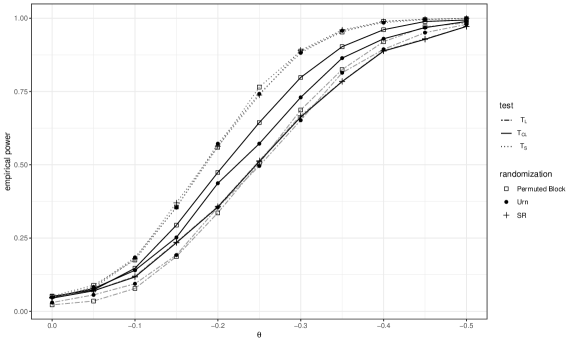
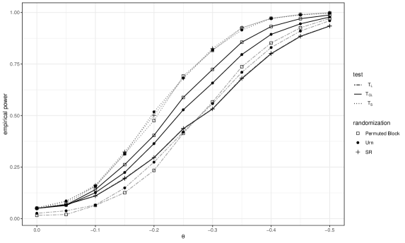
Figure 1: Empirical power evaluated for $T_{L}$, $T_{CL}$, $T_{S}$ under three different randomization schemes in Case 1 ($\alpha=5\%$, $n=500$, based on 2000 runs).

Figure 2: Empirical power evaluated for $T_{L}$, $T_{CL}$, $T_{S}$ under three different randomization schemes in Case 2 ($\alpha=5\%$, $n=500$, based on 2000 runs)

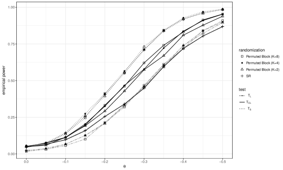
Figure 3: Empirical power evaluated for $T_{L}$, $T_{CL}$, $T_{S}$ in Case 3, with the continuous variable discretized into different number of categories ($\alpha=5\%$, $n=500$, based on 2000 runs)

The simulation Type I error based on 10,000 runs is shown in Table 1 and the simulation power based on 2,000 runs is shown in Figures 1-3. Because the bootstrap and calibrated tests have similar performances, only the calibrated tests are presented in the figures. $T_{CS}$ is also omitted from the figures because it is almost the same as $T_{S}$ when the hazard in (5) equals the true hazard function. For the ease of reading, in Figures 1-2, stratified permuted block design, stratified urn design, and simple randomization are to respectively represent $\nu_{{}_{D}}=0$, $\nu_{{}_{D}}<1$, and $\nu_{{}_{D}}=1$, while in Figure 3, only the stratified permuted block design is included in to represent covariate-adaptive randomization methods.

The following conclusions can be made from Table 1 and Figures 1-3.

• The log-rank test $T_{L}$ is conservative under covariate-adaptive randomization. Because of this conservativeness, the power of $T_{L}$ under covariate-adaptive randomization is smaller than that under simple randomization when treatment effect is small, but the trend is reversed later when treatment effect is large.

• The type I error of $T_{BL}$, $T_{CL}$, $T_{BS}$, and $T_{CS}$ under covariate-adaptive biased coin randomization, stratified permuted block randomization, and stratified urn design are close to the nominal level 5%, depicting the robustness of bootstrap and calibrated log-rank test and score test.

• Generally, the log rank type of tests $T_{L}$, $T_{BL}$, and $T_{CL}$ are not as powerful as the score type of tests $T_{S}$, $T_{BS}$, and $T_{CS}$ when model is correctly specified. This is different from the case of linear and generalized linear models (Shao et al., 2010; Shao and Yu, 2013), where the bootstrap t-test and Wald test using the same covariate information have almost the same power.

• The log rank type of tests $T_{BL}$ and $T_{CL}$ are more powerful under designs satisfying (D1) than they are under designs satisfying (D2) such as the stratified urn design and simple randomization.

• The three score tests $T_{S},T_{BS},$ and $T_{CS}$ have almost the same power under different randomization schemes, when the model is correctly specified.

• When a discretized continuous covariate is used in covariate-adaptive randomization, $T_{BL}$ and $T_{CL}$ are more powerful when the covariate is discretized into more categories. On the other hand, too many categories may cause sparsity of data in some strata.

Overall, the findings in simulation exactly coincides with asymptotic results given in Section 3.

The second simulation study aims to study the robustness and efficiency of tests when model is misspecified. The model-based score test $T_{M}$ is also included to evaluate its performance under model misspecification. Thus, there are a total of 7 tests. We consider the following three cases.

Case 4.

The true hazard $=\lambda_{0}\exp(\theta I+Z_{1}-2Z_{1}Z_{21}+Z_{1}Z_{22})$, $C\sim U(20,50)$, where $Z_{1}$, $Z_{2}$, and $Z_{2k}$ are the same as those in Case 2. The working hazard (5) is $\lambda_{0}(t)\exp(\theta I+\beta_{1}Z_{1}+\beta_{2}Z_{2})$, which is a misspecified hazard model since it does not include the interaction. $Z_{1}$ and $Z_{2}$ are used in covariate-adaptive randomization.

Case 5.

The true hazard $=\lambda_{0}\exp(\theta I-0.5Z_{1}+1.5Z_{2}^{2})$, $C|Z_{1}\sim 10+{\cal E}(2Z_{1})$, where $Z_{1}$ and $Z_{2}$ are the same as those in Case 3 and ${\cal E}(a)$ denotes the exponential distribution with mean $a$. The covariate-adaptive randomization is carried out with $Z_{1}$ and discretized $Z_{2}$ with 4 levels. The working hazard (5) is $\lambda_{0}(t)\exp(\theta I+\beta_{1}Z_{1}+\beta_{2}Z_{2})$ without recognizing that the effect of $Z_{2}$ is quadratic.

Case 6.

The failure time $X^{*}$ does not follow Cox proportional hazard model, but $X^{*}=\exp(\theta I+1.5Z)+\epsilon$, where $Z\sim N(0,1)$ and $\epsilon\sim{\cal E}(1)$ are independent. $C\sim U(10,20)$. The covariate-adaptive randomization is carried out with $Z$ discretized with 4 levels. The working hazard (5) is $\lambda_{0}(t)\exp(\theta I+\beta Z)$, which is a misspecified hazard model.

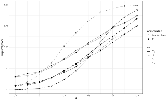
Figure 4: Empirical power evaluated for $T_{M}$, $T_{L}$, $T_{CL}$, $T_{CS}$ in Case 6. ($\alpha=5\%$, $n=500$, based on 2000 runs)

The simulation results of type I error are shown in Table 2 and the simulation results of power for Case 6 are presented in Figure 4. Several conclusions can be obtained as follows.

• The type I error for $T_{BL}$, $T_{CL}$, $T_{BS}$ and $T_{CS}$ are close to the nominal level 5% under covariate adaptive biased coin randomization, stratified permuted block randomization and stratified urn design, indicating that the proposed tests are robust to any model misspecification.

• $T_{L}$ and $T_{S}$ may be conservative when model is misspecified. Although $T_{S}$ is robust against model misspecification under simple randomization, it is not robust under covariate adaptive randomization, which agrees with our asymptotic results.

• The calibration for log-rank and score tests does not apply to Pocock and Simon’s marginal method because its asymptotic property is unfortunately unknown. But empirical results show that bootstrapping can intrinsically adapt to different randomization schemes and have good performance even under Pocock and Simon’s marginal method, although there is no theoretical confirmation for the bootstrap under the marginal method.

• When model is misspecified, the model-based score test $T_{M}$ can be conservative, and can also have inflated type I error. In other words, it is very fragile to model misspecification and can have unexpected performance.

• The calibrated score test $T_{CS}$ based on a wrong model can be less efficient than the calibrated log-rank test $T_{CL}$ without using any model.

5 Conclusions

We derive a unified theory of robust hypothesis testing against model misspecification in simple randomization and a large family of covariate-adaptive randomization. Based on that, we further study asymptotic validity, conservativeness, and efficiency of log-rank and score tests for treatment effect with survival outcome when covariate-adaptive randomization is applied. Empirical results are included to complement our theory. Our results apply to simple randomization, covariate-adaptive biased coin randomization, stratified permuted block randomization. stratified urn design, and partially to Pocock and Simon’s marginal method. The following are our main conclusions and recommendations.

• The log-rank, score, and Wald test robust against model misspecification under simple randomization are not robust under covariate-adaptive randomization, but they are conservative.

• The model-based score test or Wald test is valid only when working model equals the true model. When model is misspecified, they may have inflated type I error.

• A calibration is recommended for log-rank or score test that leads to robust tests. When the working model is true or nearly true, the calibrated score test is more powerful than the calibrated log-rank test. However, their relative performance is unknown when the model is misspecified.

• Covariate-adaptive randomization can boost efficiency by balancing treatment allocations across covariates. Among different covariate-adaptive randomization methods, those can achieve better balancedness, such as covariate-adaptive biased coin randomization and stratified permuted block randomization, lead to more powerful calibrated tests. Utilizing more covariate information in the design can also lead to more powerful calibrated tests.

• Pocock and Simon’s marginal method with score test works well if the working model equals the true model. When the working model is misspecified, however, its property is unknown, although its use together with the bootstrap performs well in empirical studies.

• Under simple randomization, the log-rank test is popular because of its robustness against model misspecification. The calibration technique developed in Section 3.2 enhances its applicability to more general and better covariate-adaptive treatment randomization designs without sacrificing robustness.

The following is a summary of the performance of various tests under simple randomization (SR) or covariate-adaptive randomization (CA). Note that Wald’s test is asymptotically equivalent to the corresponding score test.

	When hazard is misspecified					Efficiency when (5)
Method		under SR		under CA		is the true hazard
model-base score test (6)		incorrect†		incorrect†		efficient
score test (8)		robust		conservative		efficient
log-rank test (19)		robust		conservative		inefficient
calibrated score test (22)		robust		robust		efficient
calibrated log-rank test (22), $\widehat{\beta}_{0}=0$		robust		robust		partially efficient
† the type I error may be inflated

Supplemental Material

The supplemental material contains the Appendix showing proofs of technical results in the article.

Table 1: Simulation type I error in % when (5) gives the true hazard. ($\alpha=5\%$, 10,000 runs)

$n=200$ $n=500$ $T_{L}$ $T_{BL}$ $T_{CL}$ $T_{S}$ $T_{BS}$ $T_{CS}$ $T_{L}$ $T_{BL}$ $T_{CL}$ $T_{S}$ $T_{BS}$ $T_{CS}$ Case 1 Biased Coin 2.2 5.1 5.0 4.9 5.0 4.8 1.7 4.8 4.6 4.7 4.9 4.6 Permuted Block 2.0 4.8 4.7 4.5 4.6 4.4 2.2 5.4 5.1 5.2 5.2 5.1 Marginal 2.3 5.1 - 5.0 5.2 4.9 1.9 5.1 - 5.0 5.0 4.9 Urn 3.0 5.2 4.8 4.7 5.0 4.6 3.0 5.0 4.8 4.7 5.0 4.7 SR 4.7 5.0 4.5 4.9 5.1 4.9 4.6 4.8 4.5 4.8 4.9 4.8 Case 2 Biased Coin 1.9 5.3 5.8 5.0 5.2 4.9 1.6 5.0 5.0 4.9 5.0 4.8 Permuted Block 1.7 5.8 5.4 5.4 5.5 5.1 1.6 5.2 5.0 5.1 5.3 5.0 Marginal 1.9 5.3 - 5.0 4.9 4.8 1.6 5.5 - 5.1 5.0 5.0 Urn 2.7 5.3 5.0 5.6 5.7 5.4 2.6 5.2 5.0 5.3 5.4 5.2 SR 4.7 4.9 4.5 4.3 4.6 4.3 5.0 5.1 5.0 5.0 5.3 5.0 Case 3, $K=8$ Biased Coin 2.4 5.2 5.8 4.8 5.5 4.7 2.4 5.5 5.8 5.1 5.4 5.0 Permuted Block 2.0 6.2 5.5 5.4 6.1 5.3 1.7 5.5 5.2 5.3 5.8 5.2 Marginal 2.4 5.5 - 5.0 5.4 4.9 2.0 5.1 - 4.8 5.0 4.8 Urn 3.0 5.4 4.7 5.1 5.9 4.6 2.8 5.5 4.9 5.0 5.3 4.9 SR 5.0 5.2 4.8 4.9 5.2 4.9 4.7 5.0 4.6 4.7 5.1 4.7 Case 3, $K=4$ Biased Coin 2.5 5.7 6.0 4.8 5.2 4.7 2.4 5.6 5.5 4.7 5.1 4.6 Permuted Block 2.2 5.7 5.3 5.1 5.6 5.0 2.0 5.1 4.8 4.6 5.0 4.5 Marginal 2.4 5.7 - 5.3 5.6 5.2 2.3 5.6 - 5.2 5.5 5.2 Urn 3.7 6.0 5.6 5.1 5.4 4.9 3.0 5.3 4.9 4.6 4.7 4.5 SR 5.0 5.2 4.8 4.9 5.2 4.9 4.7 5.0 4.6 4.7 5.1 4.7 Case 3, $K=2$ Biased Coin 3.1 5.4 5.4 5.2 5.5 5.1 2.5 5.0 4.7 4.6 4.7 4.6 Permuted Block 2.6 5.0 4.7 4.6 4.8 4.5 2.6 5.3 4.9 5.4 5.5 5.4 Marginal 2.8 5.5 - 5.1 5.3 5.1 2.5 5.2 - 5.1 5.3 5.1 Urn 3.6 5.4 5.1 5.0 5.3 4.9 3.4 5.3 5.0 5.2 5.5 5.2 SR 5.0 5.2 4.8 4.9 5.2 4.9 4.7 5.0 4.6 4.7 5.1 4.7 $T_{L}$: log-rank test; $T_{BL}$: bootstrap log-rank test; $T_{CL}$: calibrated log-rank test $T_{S}$: score test; $T_{BS}$: bootstrap score test; $T_{CS}$: calibrated score test. Note: Under Pocock and Simon’s marginal method, $T_{CL}$ is not applicable, while $T_{CS}$ is still valid because (5) gives the true model.

Table 2: Empirical type I error in % under two model misspecification cases. ($\alpha=5\%$, based on 10,000 runs).

$n=200$ $n=500$ $T_{M}$ $T_{L}$ $T_{BL}$ $T_{CL}$ $T_{S}$ $T_{BS}$ $T_{CS}$ $T_{M}$ $T_{L}$ $T_{BL}$ $T_{CL}$ $T_{S}$ $T_{BS}$ $T_{CS}$ Case 4 Biased Coin 3.2 2.0 5.4 5.5 2.9 5.0 5.2 2.8 1.8 4.8 4.8 2.6 4.8 4.7 Permuted Block 3.0 1.8 5.6 5.1 2.9 5.2 5.0 3.0 1.7 5.0 5.1 2.8 5.2 4.9 Marginal 5.6 3.7 5.6 - 5.1 5.3 - 5.8 3.5 5.5 - 5.6 5.6 - Urn 4.0 2.7 5.4 4.9 3.7 5.3 5.1 3.6 2.9 5.6 5.3 3.5 5.3 5.1 SR 5.3 4.9 5.0 4.8 4.6 4.9 4.6 5.1 5.1 5.0 5.0 4.8 5.0 4.8 Case 5 Biased Coin 2.3 2.3 5.5 5.8 2.3 5.2 5.7 2.4 2.3 5.8 5.8 2.4 5.8 5.8 Permuted Block 2.2 2.2 6.0 5.5 2.2 5.7 5.4 2.0 1.9 5.2 5.0 2.0 5.3 5.0 Marginal 2.5 2.3 5.3 - 2.4 5.3 - 2.0 1.9 5.0 - 2.0 5.0 - Urn 2.7 2.6 5.2 4.8 2.6 5.1 4.8 3.1 2.9 5.5 5.3 3.1 5.5 5.3 SR 4.7 4.9 4.9 4.8 4.6 4.8 4.6 4.9 5.0 5.2 4.9 4.8 4.9 4.8 Case 6 Biased Coin 13.0 0.3 5.4 6.9 3.6 5.0 4.4 15.3 0.2 5.4 5.8 3.6 5.0 4.4 Permuted Block 13.6 0.1 5.9 5.7 3.6 5.2 4.3 15.3 0.1 5.3 5.1 3.9 5.5 4.7 Marginal 13.7 0.2 5.0 - 3.5 4.9 - 14.8 0.1 5.1 - 3.9 5.1 - Urn 14.0 0.9 5.4 5.1 3.4 4.5 3.8 15.7 1.0 5.6 5.4 4.1 5.1 4.6 SR 14.6 5.0 5.2 4.8 4.1 4.8 4.1 15.6 5.0 5.2 4.9 4.2 4.9 4.2 $T_{M}$: model-based Wald test; $T_{L}$: log-rank test; $T_{BL}$: bootstrap log-rank test; $T_{CL}$: calibrated log-rank test $T_{S}$: score test; $T_{BS}$: bootstrap score test; $T_{CS}$: calibrated score test. Note: $T_{CL}$ and $T_{CS}$ are not applicable under Pocock and Simon’s marginal method thus are omitted.

References

- Breugom et al. (2015) Breugom, A. J., van Gijn, W., Muller, E. W., Berglund, Å., van den Broek, C. B. M., Fokstuen, T., Gelderblom, H., Kapiteijn, E., Leer, J. W. H., Marijnen, C. A. M., Martijn, H., Meershoek-Klein Kranenbarg, E., Nagtegaal, I. D., Påhlman, L., Punt, C. J. A. et al. (2015) Adjuvant chemotherapy for rectal cancer patients treated with preoperative (chemo)radiotherapy and total mesorectal excision: a dutch colorectal cancer group (dccg) randomized phase iii trial†. Annals of Oncology, 26, 696–701. URL: http://dx.doi.org/10.1093/annonc/mdu560.
- Bugni et al. (2017) Bugni, F. A., Canay, I. A. and Shaikh, A. M. (2017) Inference under covariate-adaptive randomization. Journal of the American Statistical Association, 1–13. URL: https://doi.org/10.1080/01621459.2017.1375934.
- DiRienzo and Lagakos (2002) DiRienzo, A. G. and Lagakos, S. W. (2002) Effects of model misspecification on tests of no randomized treatment effect arising from cox’s proportional hazards model. Journal of the Royal Statistical Society: Series B (Statistical Methodology), 63, 745–757. URL: https://doi.org/10.1111/1467-9868.00310.
- Efron (1971) Efron, B. (1971) Forcing a sequential experiment to be balanced. Biometrika, 58, 403–417. URL: http://www.jstor.org/stable/2334377.
- Fakhry et al. (2015) Fakhry, F., Spronk, S., van der Laan, L. et al. (2015) Endovascular revascularization and supervised exercise for peripheral artery disease and intermittent claudication: A randomized clinical trial. JAMA, 314, 1936–1944. URL: + http://dx.doi.org/10.1001/jama.2015.14851.
- Hu and Hu (2012) Hu, Y. and Hu, F. (2012) Asymptotic properties of covariate-adaptive randomization. Ann. Statist., 40, 1794–1815. URL: https://projecteuclid.org:443/euclid.aos/1350394517.
- Kong and Slud (1997) Kong, F. H. and Slud, E. (1997) Robust covariate-adjusted logrank tests. Biometrika, 84, 847–862. URL: http://dx.doi.org/10.1093/biomet/84.4.847.
- Lin and Wei (1989) Lin, D. Y. and Wei, L. J. (1989) The robust inference for the cox proportional hazards model. Journal of the American Statistical Association, 84, 1074–1078. URL: http://www.tandfonline.com/doi/abs/10.1080/01621459.1989.10478874.
- Ma et al. (2015) Ma, W., Hu, F. and Zhang, L. (2015) Testing hypotheses of covariate-adaptive randomized clinical trials. Journal of the American Statistical Association, 110, 669–680. URL: https://doi.org/10.1080/01621459.2014.922469.
- van der Ploeg et al. (2010) van der Ploeg, A. T., Clemens, P. R., Corzo, D., Escolar, D. M., Florence, J. et al. (2010) A randomized study of alglucosidase alfa in late-onset pompe’s disease. New England Journal of Medicine, 362, 1396–1406. URL: http://dx.doi.org/10.1056/NEJMoa0909859. PMID: 20393176.
- Pocock and Simon (1975) Pocock, S. J. and Simon, R. (1975) Sequential treatment assignment with balancing for prognostic factors in the controlled clinical trial. Biometrics, 31, 103–115. URL: http://www.jstor.org/stable/2529712.
- Schulz and Grimes (2002) Schulz, K. F. and Grimes, D. A. (2002) Generation of allocation sequences in randomised trials: chance, not choice. The Lancet, 359, 515–519. URL: http://dx.doi.org/10.1016/S0140-6736(02)07683-3.
- Shao and Yu (2013) Shao, J. and Yu, X. (2013) Validity of tests under covariate-adaptive biased coin randomization and generalized linear models. Biometrics, 69, 960–969. URL: http://dx.doi.org/10.1111/biom.12062.
- Shao et al. (2010) Shao, J., Yu, X. and Zhong, B. (2010) A theory for testing hypotheses under covariate-adaptive randomization. Biometrika, 97, 347–360. URL: http://www.jstor.org/stable/25734090.
- Stott et al. (2017) Stott, D. J., Rodondi, N., Kearney, P. M., Ford, I., Westendorp, R. G., Mooijaart, S. P. et al. (2017) Thyroid hormone therapy for older adults with subclinical hypothyroidism. New England Journal of Medicine, 376, 2534–2544. URL: http://dx.doi.org/10.1056/NEJMoa1603825. PMID: 28402245.
- Struthers and Kalbfleisch (1986) Struthers, C. A. and Kalbfleisch, J. D. (1986) Misspecified proportional hazard models. Biometrika, 73, 363–369. URL: http://www.jstor.org/stable/2336212.
- Sun et al. (2018) Sun, J.-M., Lee, K. H., Kim, B.-S., Kim, H.-G., Min, Y. J., Yi, S. Y., Yun, H. J., Jung, S.-H., Lee, S.-H., Ahn, J. S., Park, K. and Ahn, M.-J. (2018) Pazopanib maintenance after first-line etoposide and platinum chemotherapy in patients with extensive disease small-cell lung cancer: a multicentre, randomised, placebo-controlled phase ii study (kcsg-lu12-07). British Journal Of Cancer. URL: http://dx.doi.org/10.1038/bjc.2017.465.
- Taves (1974) Taves, D. R. (1974) Minimization: A new method of assigning patients to treatment and control groups. Clinical Pharmacology & Therapeutics, 15, 443–453. URL: http://dx.doi.org/10.1002/cpt1974155443.
- Taves (2010) — (2010) The use of minimization in clinical trials. Contemporary Clinical Trials, 31, 180–184. URL: http://dx.doi.org/10.1016/j.cct.2009.12.005.
- Wei (1977) Wei, L.-J. (1977) A class of designs for sequential clinical trials. Journal of the American Statistical Association, 72, 382–386. URL: http://www.tandfonline.com/doi/abs/10.1080/01621459.1977.10481005.
- Wei (1978a) Wei, L. J. (1978a) The adaptive biased coin design for sequential experiments. The Annals of Statistics, 6, 92–100. URL: http://www.jstor.org/stable/2958692.
- Wei (1978b) — (1978b) An application of an urn model to the design of sequential controlled clinical trials. Journal of the American Statistical Association, 73, 559–563. URL: http://www.jstor.org/stable/2286600.
- Weir and Lees (2003) Weir, C. J. and Lees, K. R. (2003) Comparison of stratification and adaptive methods for treatment allocation in an acute stroke clinical trial. Statistics in Medicine, 22, 705–726. URL: http://dx.doi.org/10.1002/sim.1366.
- Zelen (1974) Zelen, M. (1974) The randomization and stratification of patients to clinical trials. Journal of Clinical Epidemiology, 27, 365–375. URL: http://dx.doi.org/10.1016/0021-9681(74)90015-0.