Optimization of Robot Tasks with Cartesian Degrees of Freedom using Virtual Joints

Abstract

A common task in robotics is unloading identical goods from a tray with rectangular grid structure. This naturally leads to the idea of programming the process at one grid position only and translating the motion to the other grid points, saving teaching time. However this approach usually fails because of joint limits or singularities of the robot. If the task description has some redundancies, e.g. the objects are cylinders where one orientation angle is free for the gripping process, the motion may be modified to avoid workspace problems. We present a mathematical algorithm that allows the automatic generation of robot programs for pick-and-place applications with structured positions when the workpieces have some symmetry, resulting in a Cartesian degree of freedom for the process. The optimization uses the idea of a virtual joint which measures the distance of the desired TCP to the workspace such that the nonlinear optimization method is not bothered with unreachable positions. Combined with smoothed versions of the functions in the nonlinear program higher order algorithms can be used, with theoretical justification superior to many ad-hoc approaches used so far.

I Problem Statement

We consider the following task: A robot should unload a storage box with a chess-board like structure containing $B_{x}\times B_{y}$ identical workpieces at positions $P_{kl}$, $k=1,\ldots,B_{x}$, $l=1,\ldots,B_{y}$, counted in the coordinate directions of the frame $C\in{\cal{F}}$ (where ${\cal{F}}$ denotes the set of all frames ${\mathbb{R}}^{3}\times\mbox{SO}(3)$) associated with the box at distances $D_{x}$ and $D_{y}$. Think of test-tubes in medicine or small parts in general production, as in Figure 1. The cell setup is considered fixed, also the placement of the box in the cell cannot be chosen.

Usually a pick-and-place operation is programmed at one corner only, the other position commands are computed from this corner position and the indices and distances. In this paper we consider the simplest case of a linear motion from the workpiece positions $P_{kl}$ to a position $P_{kl}+{[0,0,\Delta z]}t$ some safe distance $\Delta z$ above the grid from where the object can be moved with PTP motions which are considered “simple” in this paper so there is no need for optimization.

Figure 1: Storage boxes

We consider a standard 6-axis kinematics with central wrist where up to 8 discrete solutions of the backward transform can be calculated analytically in non-singular configurations, one of which is selected by some configuration bits in the application program. We identify these 8 configurations with an integer $s\in\{0,\ldots,7\}$. However it is difficult for the user to assess whether all positions are reachable because of nonlinearity, singularities, axis limits, cabling restricting the axes, and so on. Testing the corners is a heuristic that works in many cases but there is no guarantee, so one has to run time-consuming tests. When the process needs to work on an object from different sides or with different orientations the situation is even more complicated. So the user would like to have an algorithm that determines a feasible object frame $C$ near some initial guess $C_{0}$, maybe additionally optimizing one of the many known manipulability measures, see [9], [13].

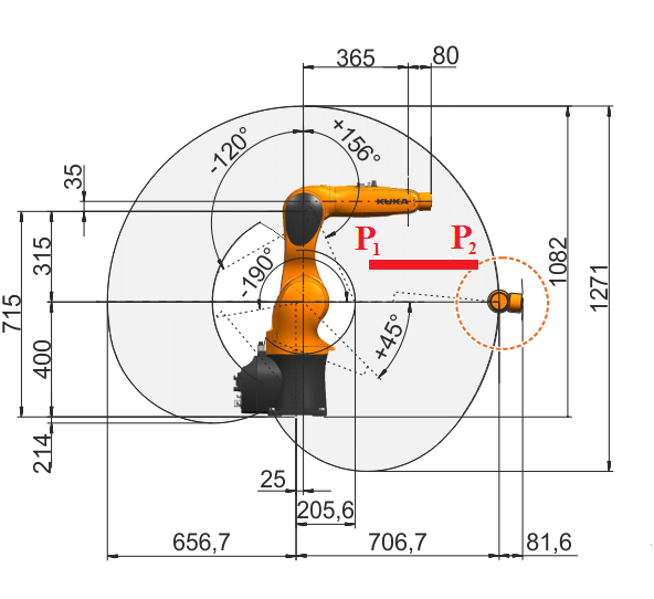
Figure 2 shows a workspace cross section of a KUKA Agilus KR 6R700 sixx industrial robot as in the manufacturer’s documentation [7] with a storage box with 2 objects only drawn as a red bar, and $P_{1}\equiv P_{1,1}\in{\mathbb{R}}^{3}$ and $P_{2}\equiv P_{1,2}\in{\mathbb{R}}^{3}$ as corners. Both points are inside the Cartesian workspace of the robot but $P_{2}$ is so close to the workspace boundary such that the flange cannot be oriented parallel to the box to lift the object along the $z$ direction. For a complete specification of the robot pose also the orientation has to be specified (plus some configuration bits). In our application the user wants the tool direction to be perpendicular to the grid box, so one degree of freedom - the orientation around the tool direction - remains for optimization. None of the state-of-the art robot programming languages offer constructs that leave one degree of freedom for optimization: The expert mode of KUKA’s KRL for example allows to leave out some components of a Cartesian point (also of axis motions), like PTP {X 450, Y 0, Z 300, A 90, B 0} where the C component of the orientation is missing, but this is only a short hand writing for “keep the current C component”. So essentially all degrees of freedom are specified. So the user has to specify a degree of freedom in a - usually - suboptimal way although it has no meaning for the process, and may even lead to unreachable poses.

Our goal is to find admissible motions for all grid points given one sample motion, where the process degree of freedom is determined by an optimizer to give admissible motions at all grid points. In order to use the standard programming languages these motions are specified by all degrees of freedom: 5 given by the grid point and the sample motion, one determined by the optimizer.

One main difficultiy arises: It is easy to check in a program whether a given frame $C$ leads to reachable positions or not like $P_{1}$ in the figure, or unreachable positions like $P_{2}$, but it is difficult for a nonlinear optimizer to determine a direction that leads to a ”more feasible” situation, starting from an infeasible one: Feasibility is a binary decision; the backward transformation will usually issue an error only, and abort.

Figure 2: Cross section of workspace with storage box

Our idea is to introduce a virtual joint as a slack variable in terms of nonlinear programming (see [10]) into the optimization problem that measures the distance of a position from feasibility; . This variable therefore has an intuitive geometric interpretation. This approach has already been applied in [12] to the optimal placement of an object in the robot workspace when there are no redundant degrees of freedom in the process.

Our approach has some similarity to the introduction of virtual axes for singularity avoidance in [11] or [6]. However we do not introduce a rotational joint to reduce velocities near singularities but rather use a prismatic joint to enlargen the mathematical workspace in the optimization process. In combination with a smooting operation we can use standard optimization algorithms which require differentiability of order 1 like all algorithms based on gradient descent, or order 2 like Sequential Quadratic Programming (SQP), cf. [10].

The paper is organzied as follows: In Section II we describe the idea of a virtual axis in the kinematics. In Section III we state the optimization problem. Section IV shows numerical results, leading to the conclusion with directions for further research in Section V.

II Virtual Axis Approach

For ease of exposition we choose a 6R robot resembling the well known Puma 560 or the KUKA Agilus but with more zeros in the parameters. We could extend all formulae to similar 6R real industrial robots. We use the DH convention

$$\hbox{R}_{z}({q_{i}})\cdot\hbox{T}_{z}({d_{i}})\cdot\hbox{T}_{x}({a_{i}})\cdot\hbox{R}_{x}({\alpha_{i}})=:\hbox{R}_{z}({q_{i}})\cdot B_{i}=:A_{i}(q_{i})$$

to get wrist centre point WCP and tool centre point TCP

$$\mbox{\sf WCP}(q) = A_{1}(q_{1})\cdot A_{2}(q_{2})\cdot A_{3}(q_{3})\cdot A_{4}(q_{4})\cdot A_{5}(q_{5})\cdot A_{6}(q_{6})$$

$$\mbox{\sf TCP}(q) = \mbox{\sf WCP}(q)\cdot\mbox{\sf TOOL}$$

expressed relative to the world coordinate system chosen as the axis 1 coordinate system.

TABLE I: DH parameters for original robot

$i$	$\theta_{i}$	$d_{i}$	$a_{i}$	$\alpha_{i}$	type
1	$q_{1}$	0	0	$\frac{\pi}{2}$	R
2	$q_{2}$	0	$l_{23}$	0	R
3	$q_{3}$	0	0	$-\frac{\pi}{2}$	R
4	$q_{4}$	$l_{35}$	0	$\frac{\pi}{2}$	R
5	$q_{5}$	0	0	$-\frac{\pi}{2}$	R
6	$q_{6}$	0	0	0	R

Figure 3: Reference position $q=0$ for original robot

Table I and Figure 3 show the robot data and the reference position. We assume joint limits $-\pi\leq q_{\min,i}\leq q_{i}\leq q_{\max,i}\leq\pi$, $i=1,\ldots 6$.

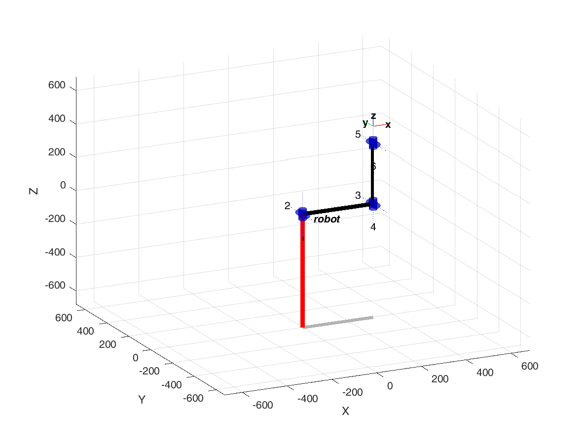
Infeasibility of the backward transform for a given frame $F$ and configuration $s$ may arise from two reasons with different severity: First, the WCP may be to far from the robot such that the triangle construction for $q_{3}$ fails. There is no remedy in this case. Second, even if axis values $q$ exist such that $\mbox{\sf TCP}(q)=F$, these might violate the joint limits: $q_{i}\not\in[q_{\min,i},q_{\max,i}]$ for some $i$. This is no obstacle during the optimization process, only for a solution. So the second problem can be fixed by dropping the joint limits and allowing $q_{i}\in(-\pi,\pi]$, $i=1,\ldots,6$.

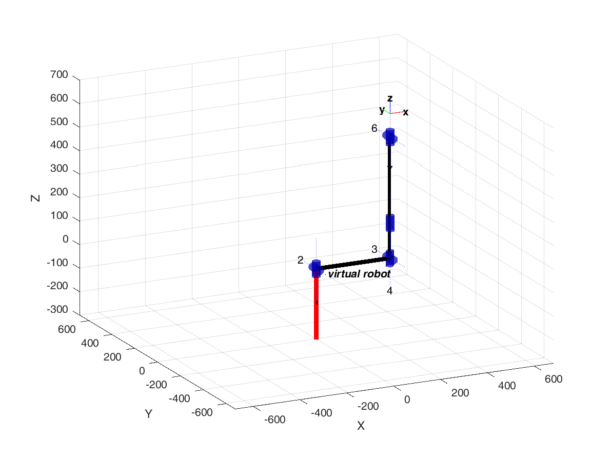
In order to use optimization algorithms which may leave the feasible set ${\cal W}_{M}$, our goal is to define a virtual robot which has a solution for the backward transform for any frame $F\in{\cal{F}}$ and any configuration $s$. So we associate to our original robot a virtual robot with an additional virtual prismatic joint between joints 3 and 4, which has no joint limits. Any WCP in ${\mathbb{R}}^{3}$ is reachable then. The variable of the virtual joint will be denoted $v$, the other joints keep their names giving a combined joint variable $\tilde{q}=(q_{1},q_{2},q_{3},v,q_{4},q_{5},q_{6})\in{\mathbb{R}}^{7}$. DH parameters of the virtual robot are shown in Table II.

TABLE II: DH parameters for virtual robot

$i$	$\theta_{i}$	$d_{i}$	$a_{i}$	$\alpha_{i}$	type
1	$\tilde{q}_{1}$	0	0	$\frac{\pi}{2}$	R
2	$\tilde{q}_{2}$	0	$l_{23}$	0	R
3	$\tilde{q}_{3}$	0	0	$-\frac{\pi}{2}$	R
4	0	$v$	0	0	P
5	$\tilde{q}_{4}$	$l_{35}$	0	$\frac{\pi}{2}$	R
6	$\tilde{q}_{5}$	0	0	$-\frac{\pi}{2}$	R
7	$\tilde{q}_{6}$	0	0	0	R

Figure 4: Reference position $\tilde{q}=(0,0,0,150,0,0,0)$ for virtual robot

Sufficient conditions for our approach are stated as two assumptions: Assumption 1 - Reachability of ${\mathbb{R}}^{3}$: The mapping of the original joints and the virtual joint to the WCP position is surjective onto ${\mathbb{R}}^{3}$. Assumption 2 - Reachability of $\mbox{SO}(3)$ Joints 4,5,6 form a central wrist parametrizing all of $\mbox{SO}(3)$, i.e. the mapping $(-\pi,\pi]^{3}\to\mbox{SO}(3)$, $(q_{4},q_{5},q_{6})\mapsto\hbox{R}_{z}({q_{4}})\cdot B_{4}\cdot\hbox{R}_{z}({q_{5}})\cdot B_{5}\cdot\hbox{R}_{z}({q_{6}})$ is surjective.

Both assumptions hold for standard 6R robots as considered here, for details see [12]. However we have introduced redundancy in our kinematics so we have to define a backward transform giving unique results. The virtual robot backward transform sets the virtual joint to the smallest absolute value such that a solution exists. In our case this is the distance between the WCP position and the workspace of the original robot which is a hollow sphere for our robot so calculations are simple. For algorithmic details see [12] again.

III Formulation of the Optimization Problem

We assume that in the unloading process of the box a linar motion in $z$ direction should be made. It is sufficient to consider a single grid point, and to build a loop repeating the optimization over all grid points.

At a single grid point $P_{0}$ we are given a frame $F$ with $P_{0}$ the position part and some orientation $Q$, as well as a target point $P_{1}$ which differs from $P_{0}$ in the $z$ component by some $\Delta z$ only, and the same associated orientation $Q$. The corresponding frames $(Q,P_{0})$ and $(Q,P_{1})$ should be connected by a linear motion. The motion geometry is parametrized by $\lambda\in[0,1]$, and discretized with step size $h=\frac{1}{N}$ at interpolating points $\lambda_{i}=i\cdot h$, $i=0,\ldots,N$, leading to frames $(Q,P_{0}+(0,0,\lambda_{i}\cdot\Delta z)$. We want to exploit the rotation around $z$ as an additional degree of freedom and introduce variables $\alpha_{0}$ and $\alpha_{1}$ for the rotations at $P_{0}$ and $P_{1}$, to be interpolated linearly by the robot controller:

$$F_{i}=(Q\cdot\hbox{R}_{z}({\alpha_{0}+\lambda_{i}\cdot(\alpha_{1}-\alpha_{0})}),P_{0}+(0,0,\lambda_{i}\cdot\Delta z).$$

The backward transform of the virtual robot gives

$$\tilde{q}^{(i)}=\tilde{q}(F_{i})=\tilde{q}(F(\alpha_{0},\alpha_{1})).$$

If the virtual joint is not needed, $v_{i}=0$, then the pose is admissible for the original robot as well. So our objective is to minimize the absolute value of $\tilde{v}_{i}$, which is expressed by

$$\min_{\alpha_{0},\alpha_{1}\in]-\pi,\pi]}\frac{1}{2}\sum_{i=0}^{n}v_{i}^{2}$$

The optimization is nonlinear as the backward transform is hidden in the computation of $\tilde{q}$. Note that the whole optimization can be generalized to more complicated motions as long as the geometric algorithms of the robot controller are known.

IV Numerical Results

We choose the tool geometry $(x,y,z)=(150,0,100)$ in our simulation. Figure 5 shows the two types of work space violations for a grid around the robot in the $z$ plane: the grid points shoud be approached with the same orientation, and some fixed configuration. Red points are outside of the robots work space, essentially unreachable for the WCP with the commanded orientation and configuration. Blue points are reachable for the WCP , but violate axis limits. Black points are reachable within the joint limits.

Figure 5: Workspace violations

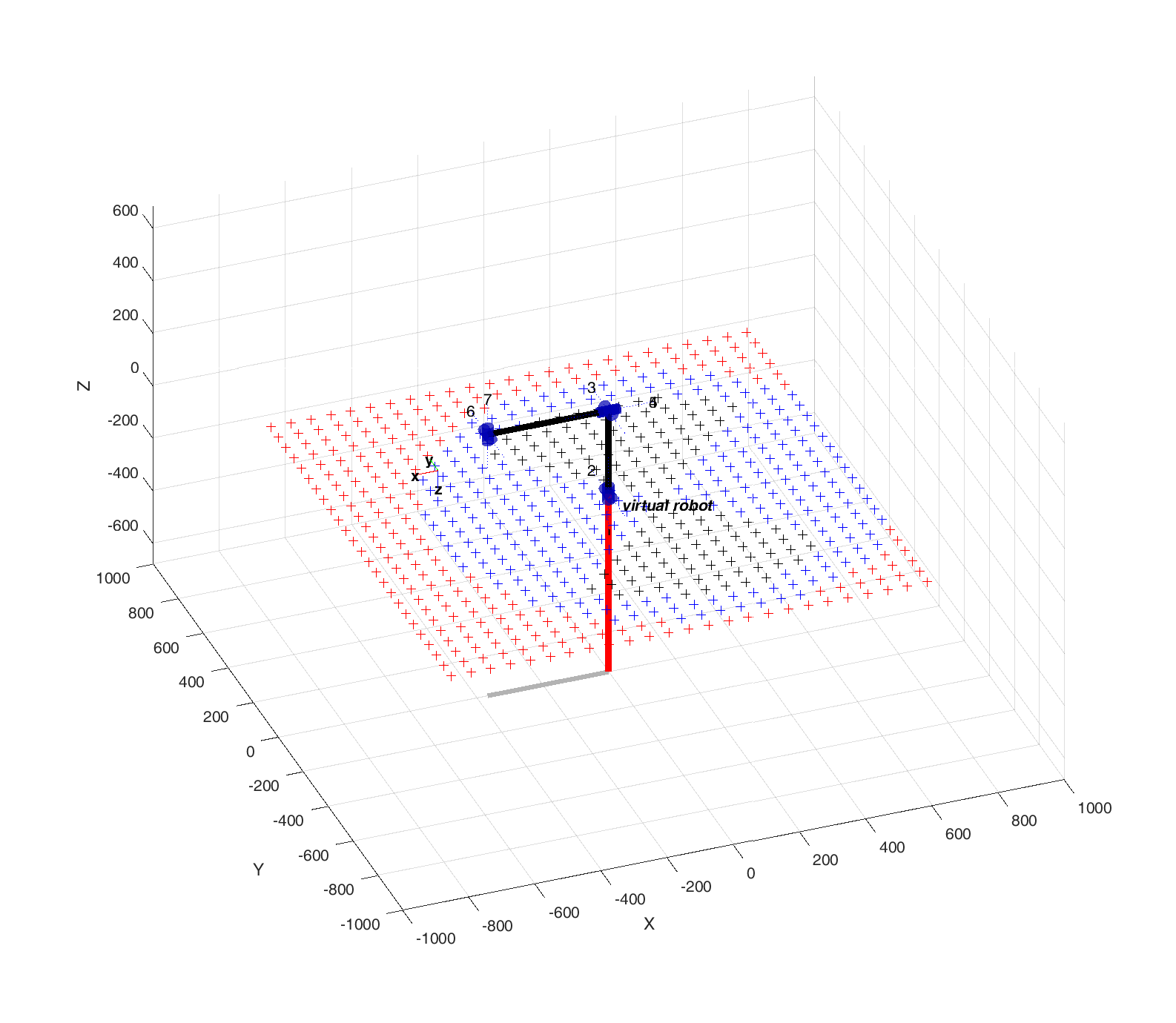
Figure 6 shows the situation from the top before and after the optimization process: Instead of the same prescribed orientation around the symmetry axis of the objects at all grid points the optimizer chooses different orientations and achieves more grid points with admissible robot poses both for WCP and axis limits, as can be seen from the increase in black locations.

Figure 6: Reachability for start point of linear motion

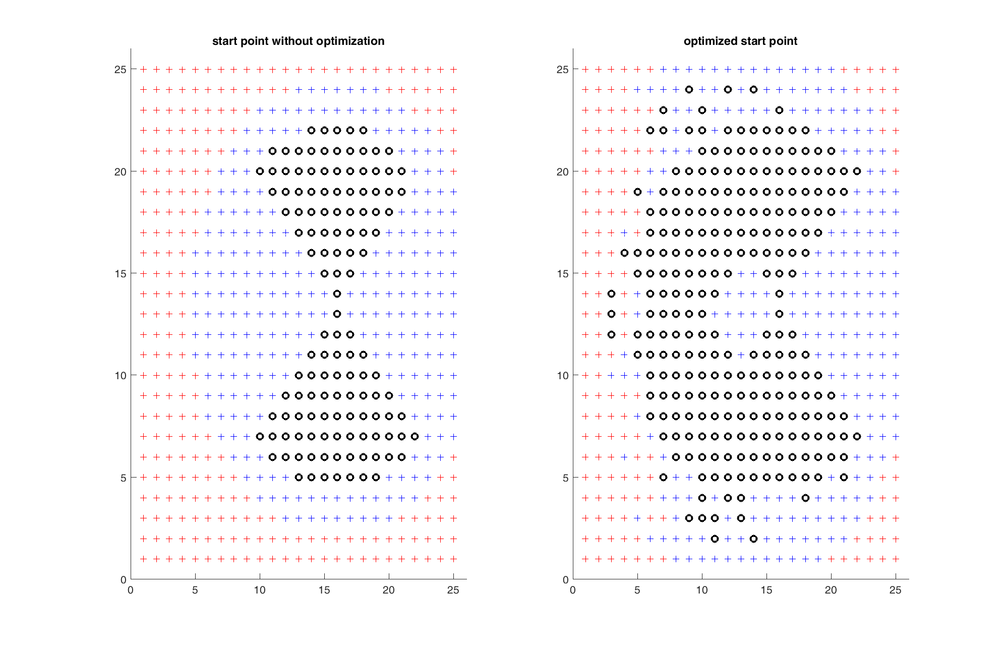
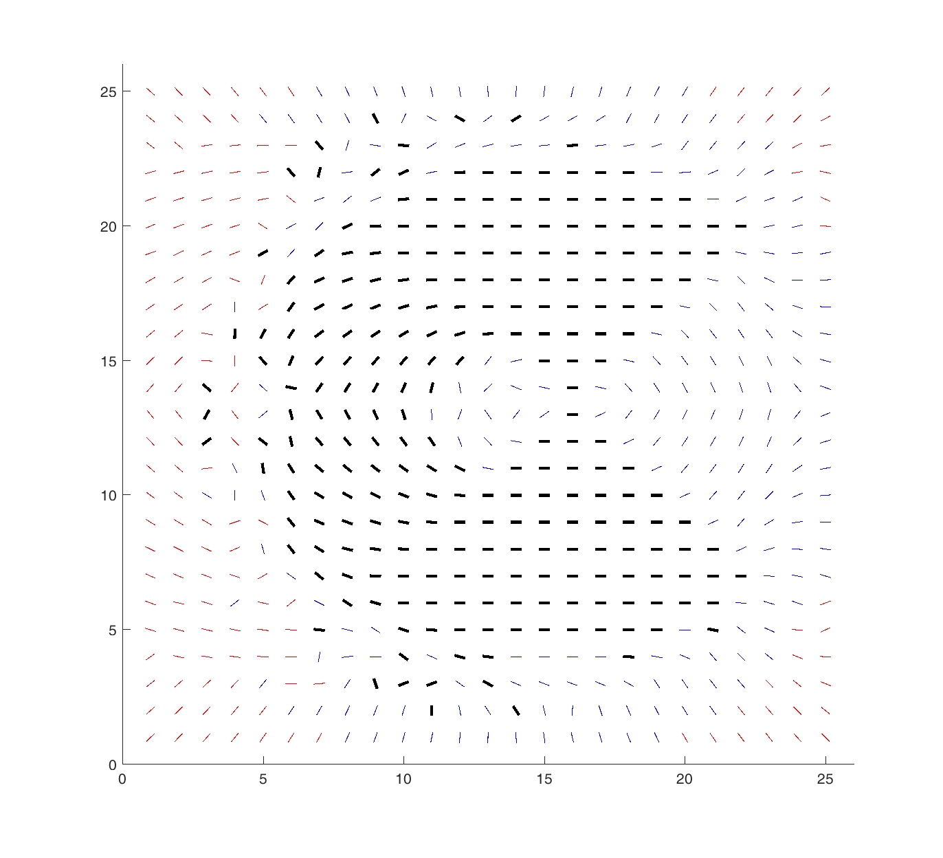
Figure 7 shows a kind of direction field representation of the chosen orientations: initially the rotational degree of freedom points to the right for all grid points. If this results in a legal pose the optimizer has no need to change anything. Otherwise the rotation around the symmetry axis is adjusted, resulting in some more legal (black) positions. For grid points where no legal pose could be found the rotation gives an direction where either the distance of the WCP to the workspace or the axis limit violation decreases.

Figure 7: Change in rotational degree of freedom by optimization

We have tested our optimization procedure with the solvers implemented in the MATLAB fmincon command. We obtained optimal solutions both with the default interior point algorithm and the SQP algorithms. However, in many cases the SQP algorithm required less iterations. Note that these algorithms require $C^{2}$ functions. The approach described so far gives a continuous but not differentiable function. In [12] a smoothing operation is explained similar to the “kinks” of [1] which overcomes this problem.

Computation time was below 10 sec on a standard laptop with $B_{x}\cdot B_{y}=25\cdot 25=625$ grid points in the box.

V Conclusions

We have shown how the virtual axis idea can be used for the optimization of processes with redundant degrees of freedom. The next natural steps are: How to select optimal motions instead of just admissible ones? This seems difficult to incorporate in the objective function. How to use this approach for robots with more than 6 axes? Here the choice of the correct configuration is a great challenge.

References

- [1] Bertsekas, D.P.: Nondifferentiable Optimization via Approximation. Math. Programming Study 3, pp. 1-25 (1975).
- [2] Craig, J.: Introduction to Robotics: Mechanics and Control. Addison Wesley, (1986)
- [3] Goppold, J.: Optimale Platzierung eines Objektes im Arbeitsraum eines Roboters, Bachelor Thesis, Ostbayerische Technische Hochschule Regensburg (2016)
- [4] KUKA Robot Group: Robots Play Board Games - Students Win Big, https://www.youtube.com/watch?v=oCQPWv_ky2c, (2016)
- [5] Léger, J., Angeles, J.: Off-line programming of six-axis robots for optimum five-dimensional tasks. Mechanism and Machine Theory 100, 155–-169 (2016)
- [6] Leontjevs, V., Flores, F.G., Lopes, J., Kecskemethy, A.: Singularity Avoidance by Virtual Redundant Axis and its Application to Large Base Motion Compensation of Serial Robots In: Proceedings of the RAAD 2012 21st International Workshop on Robotics in Alpe-Adria-Danube Region. Naples (2012)
- [7] KUKA Roboter GmbH: KR AGILUS sixx Specification. Augsburg (2013)
- [8] Léger, J., Angeles, J.: Off-line programming of six-axis robots for optimum five-dimensional tasks. Mechanism and Machine Theory 100, 155–-169 (2016)
- [9] Merlet, J.P.: Jacobian, manipulability, condition number, and accuracy of parallel robots. J. Mech. Des. 128(1), 199-–206 (2006)
- [10] Nocedal, J., Wright, S.J.: Numerical Optimization. Springer, New York (2006)
- [11] Reiter, A.: Ein Beitrag zur Singularitätsvermeidung bei Industrierobotern durch Einführung virtueller Achsen. Master Thesis, Johannes Kepler University Linz (2015)
- [12] Weiß, M.: Optimal Object Placement using a Virtual Axis, ARK 2018, 16th International Symposium on Advances in Robot Kinematics, Bologna, submitted (2018)
- [13] Yoshikawa, T.: Manipulability of Robotic Mechanisms The International Journal of Robotics Research 4(2), pp. 3-9 (1985).