^aDepartamento de Física de Altas Energias, Instituto de Ciencias Nucleares, Universidad Nacional Autónoma de México
Apartado Postal 70-543, CDMX 04510, México

^bSchool of Physics and Chemistry, Gwangju Institute of Science and Technology, Gwangju 61005, Korea

viktor.jahnke@correo.nucleares.unam.mx
viktorjahnke@gist.ac.kr

Recent developments in the holographic description of quantum chaos.

Viktor Jahnke^a,b

1 Introduction

The characterization of quantum chaos is fairly complicated. Possible approaches range from semi-classical methods to random matrix theory: in the first case one studies the semi-classical limit of a system whose classical dynamics is chaotic; in the latter approach the characterization of quantum chaos is made by comparing the spectrum of energies of the system in question to the spectrum of random matrices [1]. Despite the insights provided by the above-mentioned approaches, a complete and more satisfactory understanding of quantum chaos remains elusive.

Surprisingly, new insights into quantum chaos have come from black holes physics! In the context of so-called gauge gravity duality [2, 3, 4], black holes in asymptotically AdS spaces are dual to strongly coupled many-body quantum systems. It was recently shown that the chaotic nature of many-body quantum systems can be diagnosed with certain out-of-time-order correlation (OTOC) functions which, in the gravitational description, are related to the collision of shock waves close to the black hole horizon [5, 6, 7, 8, 9]. In addition to being useful for diagnosing chaos in holographic systems and providing a deeper understanding for the inner-working mechanisms of gauge-gravity duality, OTOCs have also proved useful in characterizing chaos in more general non-holographic systems, including some simple models like the kicked-rotor [10], the stadium billiard [11], and the Dicke model [12].

In this paper, we review the recent developments in the holographic description of quantum chaos. We discuss the characterization of quantum chaos based on the late time vanishing of OTOCs and explain how this is realized in the dual gravitational description. We also review the connections of chaos with the spreading of quantum entanglement and diffusion phenomena. We focus on the case of $d-$dimensional gravitational systems with $d\geq 3$, which excludes the case of gravity in $AdS_{2}$ and SYK-like models [13, 14, 15, 16]. Also, due the lack of the author expertise, we did not cover the recent developments in the direct field theory calculations of OTOCs. This includes calculations for CFTs [20], weakly coupled systems [21, 22], random unitary models [23, 24, 25] and spin chains [26, 27, 28, 29, 30].

2 A bird eye’s view on classical chaos

In this section we briefly review some basic aspects of classical chaos. For definiteness we consider the case of a classical thermal system with phase space denoted as ${\bf X=(q,p)}$, where ${\bf q}$ and ${\bf p}$ are multi-dimensional vectors denoting the coordinates and momenta of the phase space. We can quantify whether the system is chaotic or not by measuring the stability of a trajectory in phase space under small changes of the initial condition. Let us consider a reference trajectory in phase space, ${\bf X}(t)$, with some initial condition ${\bf X}(0)={\bf X}_{0}$. A small change in the initial condition ${\bf X}_{0}\rightarrow{\bf X}_{0}+\delta{\bf X}_{0}$ leads to a new trajectory ${\bf X}(t)\rightarrow{\bf X}(t)+\delta{\bf X}(t)$. This is illustrated in figure 1. For a chaotic system, the distance between the new trajectory and the reference one increases exponentially with time

$$|\delta{\bf X}(t)|\sim|\delta{\bf X}_{0}|e^{\lambda t}\,\,\,\text{or}\,\,\,\frac{\partial{\bf X}(t)}{\partial{\bf X}_{0}}\sim e^{\lambda t}\,,$$ (1)

where $\lambda$ is the so-called Lyapunov exponent. This should be contrasted with the behaviour of non-chaotic systems, in which $\delta{\bf X}(t)$ remains bounded or increase algebraically [31].

Figure 1: Variation of a trajectory in the phase space under small modifications of the initial condition. For a chaotic system the distance between two initially nearby trajectories increases exponentially with time, i.e., $|\delta q(t)|=|\delta q(0)|e^{\lambda t}$.

The exponential increase depends on the orientation of $\delta{\bf X}_{0}$ and this leads to a spectrum of Lyapunov exponents, $\{\lambda_{1},\lambda_{2},...,\lambda_{K}\}$, where $K$ is the dimensionality of the phase space. A useful parameter characterizing the trajectory instability is

$$\lambda_{\textrm{\tiny max}}=\lim_{t\rightarrow\infty}\lim_{\delta{\bf X}_{0}\rightarrow 0}\frac{1}{t}\log\left(\frac{\delta{\bf X}(t)}{\delta{\bf X}_{0}}\right)\,,$$ (2)

which is called the maximum Lyapunov exponent. When the above limits exist and $\lambda_{\textrm{\tiny max}}>0$ the trajectory shows sensitive to initial conditions and the system is said to be chaotic [31].

The chaotic behavior can be either a consequence of a complicated Hamiltonian or simply due to the contact with a thermal heat bath. This is because chaos is a common property of thermal systems. To later to make contact with black holes physics we consider the case of a classical thermal system with inverse temperature $\beta$. If $F({\bf X})$ is some function of the phase space coordinates we define its classical expectation value as

$$\langle F\rangle_{\beta}=\frac{\int d{\bf X}e^{-\beta H({\bf X})}F({\bf X})}{\int d{\bf X}e^{-\beta H({\bf X})}}$$ (3)

where $H({\bf X})$ is the system’s Hamiltonian.

Classical thermal systems have two exponential behaviors that have analogues in terms of black holes physics: the Lyapunov behavior, characterizing the sensitive dependence on initial conditions; and the Ruelle behavior, characterizing the approach to thermal equilibrium [32, 33].

To quantify the sensitivity to initial conditions in a thermal system we need to consider thermal expectation values. Note that (1) can have either signs. To avoid cancellations in a thermal expectation values we consider the square of this derivative

$$F(t)=\left\langle\left(\frac{\partial{\bf X}(t)}{\partial{\bf X}(0)}\right)^{2}\right\rangle_{\beta}\,.$$ (4)

The expected behavior of this quantity is the following [34]

$$F(t)\sim\sum_{k}c_{k}\,e^{2\lambda_{k}t}\,,$$ (5)

where $c_{k}$ are constants and $\lambda_{k}$ are the Lyapunov exponents. At later times the behavior is controlled by the maximum Lyapunov exponent $F\sim e^{2\lambda_{\textrm{\tiny max}}t}$.

The approach to thermal equilibrium or, in other words, how fast the system forgets its initial condition, can be quantified by two-point functions of the form

$$G(t)=\langle{\bf X}(t)\,{\bf X}(0)\rangle_{\beta}-\langle{\bf X}\rangle_{\beta}^{2}\,,$$ (6)

whose expected behavior is [34]

$$G(t)\sim\sum_{j}b_{j}\,e^{-\mu_{j}t}\,,$$ (7)

where $b_{j}$ are constants and $\mu_{j}$ are complex parameters called Ruelle resonances. The late time behavior is controlled by the smallest Ruelle resonance $G\sim e^{-\mu_{\textrm{\tiny min}}t}$.

3 Some aspects of quantum chaos

In this section, we review some aspects of quantum chaos. For a long time, the characterization of quantum chaos was made by comparing the spectrum of energies of the system in question to the spectrum of random matrices or using semiclassical methods [1]. Here we follow a different approach, which was first proposed by Larkin and Ovchinnikov [35] in the context of semi-classical systems, and it was recently developed by Shenker and Stanford [6, 7, 8] and by Kitaev [9].

For simplicity, let us consider the case of a one-dimensional system, with phase space variables $(q,p)$. Classically, we know that $\partial q(t)/\partial q(0)$ grows exponentially with time for a chaotic system. The quantum version of this quantity can be obtained by noting that

$$\frac{\partial q(t)}{\partial q(0)}=\{q(t),p(0)\}_{\textrm{\tiny P.B.}}\,,$$ (8)

where $\{q(t),p(0)\}_{\textrm{\tiny P.B.}}$ denotes the Poisson bracket between the coordinate $q(t)$ and the momentum $p(0)$. The quantum version of $\partial q(t)/\partial q(0)$ can then be obtained by promoting the Poisson bracket to a commutator

$$\{q(t),p(0)\}_{\textrm{\tiny P.B.}}\rightarrow\frac{1}{i\hbar}[\hat{q}(t),\hat{p}(0)]$$ (9)

where now $\hat{q}(t)$ and $\hat{p}(0)$ are Heisenberg operators.

We will be interested in thermal systems, so we would like to calculate the expectation value of $[\hat{q}(t),\hat{p}(0)]$ in a thermal state. However, this commutator might have either sign in a thermal expectation value and this might lead to cancellations. To overcome this problem, we consider the expectation value of the square of this commutator

$$C(t)=\left\langle-[\hat{q}(t),\hat{p}(0)]^{2}\right\rangle_{\beta}\,,$$ (10)

where $\beta$ is the system’s inverse temperature and the overall sign is introduced to make $C(t)$ positive. More generally, one might replace $\hat{q}(t)$ and $\hat{p}(0)$ by two generic hermitian operators $V$ and $W$ and quantify chaos with the double commutator

$$C(t)=\left\langle-[W(t),V(0)]^{2}\right\rangle_{\beta}\,.$$ (11)

This quantity measures how much an early perturbation $V$ affects the later measurement of $W$. As chaos means sensitive dependence on initial conditions, we expect $C(t)$ to be ‘small’ in non-chaotic system, and ‘large’ if the dynamics is chaotic. In the following, we give a precise meaning for the adjectives ‘small’ and ‘large’.

For some class of systems, the quantum behavior of $C(t)$ has a lot of similarities with the classical behavior of $\langle(\partial q(t)/\partial q(0))\rangle_{\beta}$. However, the analogy between the classical and quantum quantities is not perfect because there is not always a good notion of a small perturbation in the quantum case (remember that classical chaos is characterized by the fact that a small perturbation in the past has important consequences in the future). If we start with some reference state and then perturb it, we easily produce a state that is orthogonal to the original state, even when we change just a few quantum numbers. Because of that, it seems unnatural to quantify the perturbation as small. Fortunately, there are some quantum systems in which the notion of a small perturbation makes perfect sense. An example is provided by systems with a large number of degrees of freedom. In this case, a perturbation involving just a few degrees of freedom is naturally a small perturbation.

For some class of chaotic systems, which include holographic systems, $C(t)$ is expected to behave as

$$C(t)\sim\begin{cases}N_{\textrm{\tiny dof}}^{-1}&\quad\text{for }\,\,t<t_{d}\,,\\ N_{\textrm{\tiny dof}}^{-1}\exp\left(\lambda_{L}t\right)&\quad\text{for}\,\,t_{d}<\!\!<t<\!\!<t_{*}\\ \mathcal{O}(1)&\quad\text{for}\,\,t>t_{*}\,,\end{cases}$$

where $N_{\textrm{\tiny dof}}$ is the number of degrees of freedom of the system. Here, we have assumed $V$ and $W$ to be unitary and hermitian operators, so that $VV=WW=1$. The exponential growth of $C(t)$ is characterized by the Lyapunov exponent $\lambda_{L}$ and takes place at intermediate time scales bounded by the dissipation time $t_{d}$ and the scrambling time $t_{*}$. The dissipation time is related to the classical Ruelle resonances ($t_{d}\sim\mu^{-1}$) and it characterizes the exponential decay of two-point correlators, e.g., $\langle V(0)V(t)\rangle\sim e^{-t/t_{d}}$. The dissipation time also controls the late time behavior of $C(t)$. The scrambling time $t_{*}\sim\lambda_{L}^{-1}\log N_{\textrm{\tiny dof}}$ is defined as the time at which $C(t)$ becomes of order $\mathcal{O}(1)$. See figure 2. The scrambling time controls how fast the chaotic system scrambles information. If we perturb the system with an operator that involves only a few degrees of freedom, the information about this operator will spread among the other degrees of freedom of the system. After a scrambling time, the information will be scrambled among all the degrees of freedom and the operator will have a large commutator with almost any other operator.

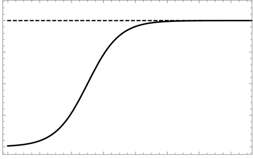
Figure 2: Schematic form of $C(t)$. We indicated the regions of Lyapunov and Ruelle behavior. $C(t)\sim\mathcal{O}(1)$ at $t\sim t_{*}$.

To understand how the above behavior relates to chaos, we write the double commutator as

$$C(t) = \left\langle-[W(t),V(0)]^{2}\right\rangle_{\beta}$$ (12)

$$= 2-2\,\langle W(t)V(0)W(t)V(0)\rangle_{\beta}\,,$$ (13)

where we made the assumption that $W$ and $V$ are hermitian and unitary operators. Note that all the relevant information about $C(t)$ is contained in the OTOC

$$\text{OTO}(t)=\left\langle W(t)V(0)W(t)V(0)\right\rangle\,.$$ (14)

The fact that $C(t)$ approaches 2 at later times implies that the OTO$(t)$ should vanish in that limit. To understand why this is related to chaos we think of OTO$(t)$ as an inner-product of two states

$$\text{OTO}(t)=\langle\psi_{2}|\psi_{1}\rangle\,,$$ (15)

where

$$|\psi_{1}\rangle=W(-t)V(0)|\beta\rangle\,,\,\,\,\,|\psi_{2}\rangle=V(0)W(-t)|\beta\rangle$$ (16)

where $|\beta\rangle$ is some thermal state and we replace $t\rightarrow-t$ to make easier the comparison with black holes physics.

If $[V(0),W(t)]\approx 0$ for any value of $t$, the two states are approximately the same, and $\langle\psi_{1}|\psi_{2}\rangle\ \approx 1$, implying $C(t)\approx 0$. That means the system displays no chaos - the early measurement of $V$ has no effect on the later measurement of $W$. If, on the other hand, $[V(0),W(t)]\neq 0$, the states $|\psi_{1}\rangle$ and $|\psi_{2}\rangle$ will have a small superposition $\langle\psi_{1}|\psi_{2}\rangle\ \approx 0$, implying $C(t)\approx 2$. That means that $V$ has a large effect on the later measurement of $W$.

In figure 3 we construct the states $|\psi_{1}\rangle$ and $|\psi_{2}\rangle$ and explain why $\langle\psi_{1}|\psi_{2}\rangle\ \approx 0$ for large $t$ means chaos. Let us start by constructing the state $|\psi_{1}\rangle=W(-t)V(0)|\beta\rangle=e^{-iHt}W(0)e^{iHt}V(0)|\beta\rangle$. The unperturbed thermal state is represented by a horizontal line. We initially consider the state $V(0)|\beta\rangle$, which is the thermal state perturbed by $V$. If we evolve the system backward in time (applying the operator $e^{iHt}$) for some time which is larger than the dissipation time, the system will thermalize and it will no longer display the perturbation $V$. After that, we apply the operator $W$, which should be thought of as a small perturbation, and then we evolve the system forwards in time (applying the operator $e^{-iHt}$). The final result of this set of operations depends on the nature of the system. If the system is chaotic, the perturbation $W$ will have a large effect after a scrambling time, and the perturbation that was present at $t=0$ will no longer re-materialize. This is illustrated in figure 3. In contrast, for a non-chaotic system, the perturbation $W$ will have little effect on the system at later times, and the perturbation $V$ will (at least partially) re-materialize at $t=0$.

We now construct the state $|\psi_{2}\rangle=V(0)W(-t)|\beta\rangle=V(0)e^{-iHt}W(0)e^{iHt}|\beta\rangle$. This is illustrated in figure 4. We start with the thermal state $|\beta\rangle$ and then we evolve this state backwards in time $e^{iHt}|\beta\rangle$. After that we apply the operator $W$ and then we evolve the system forwards in time, obtaining the state $e^{-iHt}W(0)e^{iHt}|\beta\rangle$. Finally, we apply the operator $V$, obtaining the state $V(0)W(-t)|\beta\rangle$. Note that, by construction, this state displays the perturbation $V$ at $t=0$, while the state $W(-t)V(0)|\beta\rangle$ does not. As a consequence, the two states are expected to have a small superposition $\langle W(-t)V(0)|W(-t)V(0)\rangle_{\beta}\approx 0$. This should be contrasted to the case where the system is not chaotic. In this case the perturbation $V$ re-materializes at $t=0$, and the states $|\psi_{1}\rangle$ and $|\psi_{2}\rangle$ have a large superposition, i.e., $\langle W(-t)V(0)|W(-t)V(0)\rangle_{\beta}\approx 1$.

In this construction we assumed the operators $V(0)$ and $W(-t)$ to be separated by a scrambling time, i.e., $|t|>t_{*}$. This is important because, at earlier times, the two operators, which in general involve different degrees of freedom of the system, generically commute. The operators manage to have a non-zero commutator at later times because of the phenomenon of operation growth that we will describe in the next section.

Figure 3: Construction of the state $W(-t)V(0)|\beta\rangle$. For a chaotic system the perturbation $V$ fails to re-materialize at $t=0$. In a non-chaotic system we expect the perturbation $V$ to re-materialize at $t=0$.

Figure 4: Construction of the state $V(0)W(-t)|\beta\rangle$. By construction, this state displays the perturbation $V$ at $t=0$.

3.1 Operator growth and scrambling

The operators $V$ and $W$ act generically at different parts of the physical system, yet they can have a non-zero commutator at later times. This is possible because in chaotic systems the time evolution of an operator makes it more and more complicated, involving and increasing number of degrees of freedom. As a result, an operator that initially involves just a few degrees of freedom becomes delocalized over a region that grows with time. The growth of the operator $W(t)$ is maybe more evident from the point of view of the Baker-Campbell-Hausdorff (BCH) formula, in terms of which we can write

$$W(t)=e^{iHt}W(0)e^{-iHt}=\sum_{k=0}^{\infty}\frac{(-it)^{k}}{k!}[H[H,...[H,W(0)]...]\,]\,.$$ (17)

From the above formula it is clear that, at each order in $t$ there is a more complicated contribution to $W(t)$. In chaotic systems the operator becomes more and more delocalized as the time evolves, and it eventually becomes delocalized over the entire system. The time scale at which this occurs is the so-called scrambling time $t_{*}$. After the scrambling time the operator $W(t)$ manages to have a non-zero and large commutator with almost any other operator, even operators involving only a few degrees of freedom.

This can be clearly illustrated in the case of a spin-chain. Let us follow [7] and consider an Ising-like model with Hamiltonian

$$H=-\sum_{i}\left(Z_{i}Z_{i+1}+gX_{i}+hZ_{i}\right)\,,$$ (18)

where $X_{i},Y_{i}$ and $Z_{i}$ denote Pauli matrices acting on the $i$th site of the spin chain. The above system is integrable if we take $g=1$ and $h=0$, but it is strongly chaotic if we choose $g=-1.05$ and $h=0.5$.

To illustrate the concept of scrambling, we consider the time evolution of the operator $Z_{1}$. Using the BCH formula we can write

$$Z_{1}(t)=Z_{1}-it[H,Z_{1}]-\frac{t^{2}}{2!}[H,[H,Z_{1}]\,]+\frac{it^{3}}{3!}[H,[H,[H,Z_{1}]\,]\,]+...$$ (19)

Ignoring multiplicative constants and signs we can write the above terms (schematically) as

$$[H,Z_{1}]\sim Y_{1}$$ (20)

$$[H,[H,Z_{1}]\,]\sim Y_{1}+X_{1}Z_{2}$$

$$[H,[H,[H,Z_{1}]]]\sim Y_{1}+Y_{2}X_{1}+Y_{1}Z_{2}$$

$$[H,[H,[H,[H,Z_{1}]]]]\sim X_{1}+Y_{1}+Z_{1}+X_{1}X_{2}+Y_{1}Y_{2}+Z_{1}Z_{2}+X_{1}Z_{2}+$$

$$+Z_{3}Y_{1}+Y_{1}Z_{2}Y_{2}+Z_{1}X_{2}X_{1}+X_{2}Z_{3}X_{1}$$

As the the time evolves higher order terms become important in the series (19), and the operator $Z_{1}(t)$ becomes more and more complicated, involving terms in an increasing number of sites. For large enough $t$ the operator will involve all the sites of the spin chain and it will manage to have a non-zero commutator with a Pauli operator in any other site of the system. In this situation the information about $Z_{1}$ is essentially scramble among all the degrees of freedom of the system. As discussed before, this occurs after a scrambling time. Above this time the double commutator $C(t)$ saturates to a constant value. This should be contrasted to what happens for an integrable system. In this case the operator grows, but it also decreases at later times. In the chaotic case, the operator remains large at later times [7].

3.2 Probing chaos with local operators

In quantum field theories we can upgrade (11) to the case where the operators are separated in space

$$C(t,x)=\langle-[V(0,0),W(t,x)]^{2}\rangle_{\beta}\,.$$ (21)

Strictly speaking, the above expression is generically divergent, but it can be regularized by adding imaginary times to the time arguments of the operators $V$ and $W$. For a large class of spin-chains, higher dimensional SYK-models and CFTs the above commutator is roughly given by

$$C(t,x)\sim\exp\left[\lambda_{L}\left(t-t_{*}-\frac{|x|}{v_{B}}\right)\right]\,,$$ (22)

where $v_{B}$ is the so-called butterfly velocity. This velocity describes the growth of the operator $W$ in physical space and it acts as a low-energy Lieb-Robinson velocity [37], which sets a bound for the rate of transfer of quantum information. From the above formula, we can see that there is an additional delay in scrambling due to the physical separation between the operators. The butterfly velocity defines an effective light-cone for the commutator (21). Inside the cone, for $t-t_{*}\geq|x|/v_{B}$, we have $C(t,x)\sim\mathcal{O}(1)$, whereas for outside the cone, for $t-t_{*}<|x|/v_{B}$, the commutator is small, $C(t,x)\sim 1/N_{\textrm{\tiny dof}}<<1$. Outside the light-cone the Lorentz invariance implies a zero commutator. The light-cone and the butterfly effect cone are illustrated in figure 5.

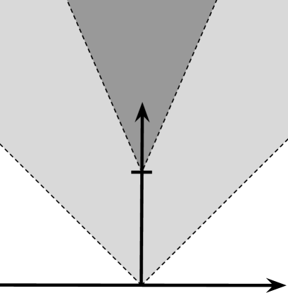
Figure 5: Light cone (gray region) and butterfly effect cone (dark gray region). Inside the butterfly effect cone, for $t-t_{*}\geq|x|/v_{B}$, we have $C(t,x)\sim\mathcal{O}(1)$, whereas for outside the cone, for $t-t_{*}<|x|/v_{B}$, the commutator is small, $C(t,x)\sim 1/N_{\textrm{\tiny dof}}<<1$. Outside the light-cone the Lorentz invariance implies a zero commutator.

4 Chaos $\&$ Holography

In this section, we review how the chaotic properties of holographic theories can be described in terms of black holes physics. Black holes behave as thermal systems and thermal systems generically display chaos. This implies that black holes are somehow chaotic. This statement has a precise realization in the context of the gauge/gravity duality. According to this duality, some strongly coupled non-gravitational systems are dual to higher dimensional gravitational systems. In the most known and studied example of this duality the $\mathcal{N}=4$ super Yang-Mills (SYM) theory living in $R^{3,1}$ is dual to type IIB supergravity in $AdS_{5}\times S^{5}$. More generically, a $d-$dimensional non-gravitational theory living in $R^{d-1,1}$ is dual to a gravity theory living in a higher-dimensional space of the form $AdS_{d+1}\times\mathcal{M}$, where $\mathcal{M}$ is generically a compact manifold. The non-gravitational theory can be thought as living in the boundary of $AdS_{d+1}$ and because of that is usually called the boundary theory. The gravitational theory is also called the bulk theory.

There is a dictionary relating physical quantities in the boundary and bulk description [3, 4]. An example is provided by the operators of the boundary theory, which are related to bulk fields. The boundary theory at finite temperature can be described by introducing a black hole in the bulk. The thermalization properties of the boundary theory have a nice visualization in terms of black holes physics. By applying a local operator in the boundary theory we produce some perturbation that describes a small deviation from the thermal equilibrium. The information about $V(x)$ is initially contained around the point $x$, but it gets delocalized over a region that increases with time until it completely melts into the thermal bath. In the bulk theory, the application of the operator $V(x)$ produces a particle (field excitation) close to the boundary of the space, which then falls into the black hole. The return to the thermal equilibrium in the boundary theory corresponds to the absorption of the bulk particle by the black hole. Figure 6 illustrates the bulk description of thermalization.

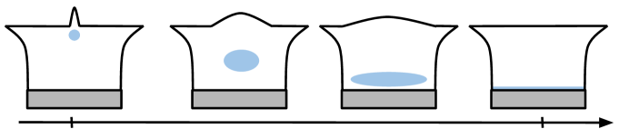
Figure 6: Bulk picture of thermalization. The figure represents an asymptotically $AdS$ black hole geometry. The boundary is at the top edge, while the black hole horizon is at the bottom edge. The black hole’s interior is shown in gray. The boundary operator $V$ is dual to the bulk field $\phi$. From the point of view of the boundary theory the perturbation produced by $V$ is initially localized around the point $x$, but it gets delocalized over a region that increases with time. In the bulk description this is described by a particle (field excitation) that is initially close to the boundary and then falls into the black hole.

The approach to thermal equilibrium is controlled by the black hole’s quasi-normal modes (QNMs). In holographic theories, the quasi-normal modes control the decay of two-point functions of the boundary theory

$$\langle V(t)V(0)\rangle_{\beta}\sim e^{-t/t_{d}}$$ (23)

where the dissipation time $t_{d}$ is related to the lowest quasi-normal mode ($\text{Im}(\omega)\sim t_{d}^{-1}$). From the point of view of the bulk theory the QNMs describes how fast a perturbed black hole returns to equilibrium. Clearly, the black hole’s quasi-normal modes correspond to the classical Ruelle resonances. In holographic theories the dissipation time is roughly give by $t_{d}\sim\beta$.

Another important exponential behavior of black holes is provided by the blueshift suffered by the in-falling quanta, or, equivalently, the red shift suffered by the quanta escaping from the black hole. The blueshift suffered by the in-falling quanta is determined by the black hole’s temperature. If the quanta asymptotic energy is $E_{0}$, this energy increases exponentially with time

$$E=E_{0}\,e^{\frac{2\pi}{\beta}t}\,,$$ (24)

where $\beta$ is the Hawking’s inverse temperature. Later we will see that this exponential increase in the energy of the in-falling quanta gives rise to the Lyapunov behavior of $C(t,x)$ of holographic theories.

4.1 Holographic setup

The TFD state $\&$ Two-sided black holes

In the study of chaos is convenient to consider a thermofield double state made out of two identical copies of the boundary theory

$$|\text{TFD}\rangle=\frac{1}{Z^{1/2}}\sum_{n}e^{-\beta E_{n}/2}|n\rangle_{\textrm{\tiny L}}|n\rangle_{\textrm{\tiny R}}\,,$$ (25)

where $L$ and $R$ label the states of the two copies, which we call $\text{QFT}_{\textrm{\tiny L}}$ and $\text{QFT}_{\textrm{\tiny R}}$, respectively. The two boundary theories do not interact and only know about each other through their entanglement. This state is dual to an eternal (two-sided) black hole, with two asymptotic boundaries, where the boundary theories live [38]. This is a wormhole geometry, with an Einstein-Rosen bridge connecting the two sides of the geometry. The wormhole is not traversable, which is consistent with the fact that the two boundary theories do not interact.

For definiteness we assume a metric of the form

$$ds^{2}=-G_{tt}(r)dt^{2}+G_{rr}(r)dr^{2}+G_{ij}(r,x^{k})dx^{i}dx^{j}\,,$$ (26)

where the boundary is located at $r=\infty$, where the above metric is assumed to asymptote $AdS_{d+1}$. We take the horizon as located at $r=r_{\textrm{\tiny H}}$, where $G_{tt}$ vanish and $G_{rr}$ has a first order pole. For future purposes, let $\beta$ be the Hawking’s inverse temperature, and $S_{\textrm{\tiny BH}}$ be the Bekenstein-Hawking entropy.

In the study of shock waves is more convenient to work with Kruskal-Szekeres coordinates, since these coordinate cover smoothly the globally extended spacetime. We first define the tortoise coordinate

$$dr_{*}=\sqrt{\frac{G_{rr}}{G_{tt}}}dr\,,$$ (27)

and then we introduce the Kruskal-Szekeres coordinates $U,V$ as

$$U = +e^{\frac{2\pi}{\beta}\left(r_{*}-t\right)}\,,\,\,V=-e^{\frac{2\pi}{\beta}\left(r_{*}+t\right)}\,\,\,(\text{left exterior region})$$

$$U = -e^{\frac{2\pi}{\beta}\left(r_{*}-t\right)}\,,\,\,V=+e^{\frac{2\pi}{\beta}\left(r_{*}+t\right)}\,\,\,(\text{right exterior region})$$ (28)

$$U = +e^{\frac{2\pi}{\beta}\left(r_{*}-t\right)}\,,\,\,V=+e^{\frac{2\pi}{\beta}\left(r_{*}+t\right)}\,\,\,(\text{future interior region})$$

$$U = -e^{\frac{2\pi}{\beta}\left(r_{*}-t\right)}\,,\,\,V=-e^{\frac{2\pi}{\beta}\left(r_{*}+t\right)}\,\,\,(\text{past interior region})$$

In terms of these coordinates the metric reads

$$ds^{2}=2A(UV)dUdV+G_{ij}(UV)dx^{i}dx^{j}\,,$$ (29)

where

$$A(UV)=\frac{\beta^{2}}{8\pi^{2}}\frac{G_{tt}(UV)}{UV}\,.$$ (30)

In these coordinates the horizon is located at $U=0$ or at $V=0$. The left and right boundaries are located at $UV=-1$ and the past and future singularities at $UV=1$. The Penrose diagram for this metric is shown in figure 7.

Figure 7: Penrose diagram for the two-sided black holes with two boundaries that asymptote $AdS$. This geometry is dual to a thermofield double state constructed out of two copies of the boundary theory.

The global extended spacetime can also be described in terms of complexified coordinates [39]. In this case one defines the complexified Schwarzschild time

$$t=t_{\textrm{\tiny L}}+i\,t_{\textrm{\tiny E}}\,,$$ (31)

where $t_{\textrm{\tiny L}}$ and $t_{\textrm{\tiny E}}$ are the Lorentzian and Euclidean times, and then one describes the time in each of the four patches (left and right exterior regions, and the future and past interior regions) as having a constant imaginary part

$$t_{\textrm{\tiny E}} = 0\,\,\,\,\,\,\,(\text{right exterior region})$$

$$t_{\textrm{\tiny E}} = -\beta/4\,\,\,(\text{future interior region})$$ (32)

$$t_{\textrm{\tiny E}} = -\beta/2\,\,\,(\text{left exterior region})$$

$$t_{\textrm{\tiny E}} = +\beta/4\,\,\,(\text{past interior region})$$

The Euclidean time has a period of $\beta$. The Lorentzian time increases upward (downward) in the right (left) exterior region, and to the right (left) in the future (past) interior.

Note that, with the complexified time, one can obtain an operator acting on the left boundary theory by adding (or subtracting) $i\beta/2$ to the time of an operator acting on the right boundary theory.

Perturbations of the TFD state $\&$ Shock wave geometries

We now turn to the description of states of the form

$$W(t)|\text{TFD}\rangle$$ (33)

where $W$ is a thermal scale operator that acts on the right boundary theory. This state can be describe by a ‘particle’ (field excitation) in the bulk that comes out of the past horizon, reaches the right boundary at time $t$, and then falls into the future horizon, as illustrated in figure 8.

Figure 8: Bulk description of the state $W(t)|\text{TFD}\rangle$. In blue is shown the trajectory of a ‘particle’ that comes out of the past horizon, reaches the boundary at time $t$ producing the perturbation $W$, and then falls into the future horizon. For now on, we will refer to this bulk excitation as the W-particle.

If $|t|$ is not too large, the state $W(t)|\text{TFD}\rangle$ will represent just a small perturbation of the TFD state and the corresponding description in the bulk will be just an eternal two-sided black hole geometry slightly perturbed by the presence of a probe particle. This is no longer the case if $|t|$ is large. In this case, there is a non-trivial modification of the geometry. A very early perturbation, for example, is described in the bulk in terms of a particle that falls towards the future horizon for a very long time and gets highly blueshifted in the process. If the particle’s energy is $E_{0}$ in the asymptotic past, this energy will be exponentially larger from the point of view of the $t=0$ slice of the geometry, i.e., $E=E_{0}\,e^{\frac{2\pi}{\beta}t}$. Therefore, for large enough $|t|$, the particle’s energy will be very large and one needs to include the corresponding back-reaction.

The back-reaction of a very early (or very late) perturbation is actually very simple - it corresponds to a shock wave geometry [40, 41]. To understand that, we first need to notice that, under boundary time evolution, the stress-energy of a generic perturbation $W$ gets compressed in the $V-$direction, and stretched in the $U-$direction. For large enough $|t|$ we can approximate the stress tensor of the W-particle as

$$T_{VV}\sim P^{U}\delta(V)a(\vec{x})\,,$$ (34)

where $P^{U}\sim\beta^{-1}e^{\frac{2\pi}{\beta}t}$ is the momentum of the W-particle in the $U-$direction and $a(\vec{x})$ is some generic function that specifies the location of the perturbation in the spatial directions of the right boundary. Note that $T_{VV}$ is completely localized at $V=0$ and homogeneous along the $U-$direction. Besides that, even if the W-particle is massive, the exponential blue-shift will make it follow an almost null trajectory, as shown in figure 9.

Figure 9: Bulk description of the state $W(-t)|\text{TFD}\rangle$. An early enough perturbation produces a shock wave geometry. The effect of the shock wave (shown in blue) is to produce a shift $U\rightarrow U+h(t,\vec{x})$ in the trajectory of a probe particle (shown in red) crossing it.

The shock wave geometry produced by the W-particle is described by the metric

$$ds^{2}=2A(UV)dUdV+G_{ij}(UV)dx^{i}dx^{j}-2A(UV)h(t,\vec{x})\delta(V)dV^{2}\,,$$ (35)

that is completely specified by the shock wave transverse profile $h(t,\vec{x})$. This geometry can be seen as two pieces of a eternal black hole glued together along $V=0$ with a shift of magnitude $h(t,\vec{x})$ in the $U-$direction. We find it useful to represent this geometry with the same Penrose diagram of the unperturbed geometry, but with the prescription that any trajectory crossing the shock wave gets shifted in the $U-$direction as $U\rightarrow U+h(t,\vec{x})$. See figure 9.

The precise form of $h(t,\vec{x})$ can be determined by solving the $VV-$component of Einstein’s equation. For a local perturbation, i.e., $a(\vec{x})=\delta^{d-1}(\vec{x})$, the solution reads

$$h(t,\vec{x})\sim G_{\textrm{\tiny N}}\,e^{\frac{2\pi}{\beta}t-\mu|\vec{x}|}\,,\,\,\,\,\text{with}\,\,\mu=\frac{2\pi}{\beta}\sqrt{\frac{(d-1)G^{\prime}_{ii}(r_{\textrm{\tiny H}})}{G^{\prime}_{tt}(r_{\textrm{\tiny H}})}}\,,$$ (36)

where, for simplicity, $G_{ij}$ has been assumed to be diagonal and isotropic.

Interestingly, the shock wave profile contains information about the parameters characterizing the chaotic behavior of the boundary theory. Indeed, the double commutator has a region of exponential growth at which $C(t,\vec{x})\sim h(t,\vec{x})$. From this identification, we can write

$$h(t,\vec{x})\sim e^{\frac{2\pi}{\beta}\left(t-t_{*}-\frac{|\vec{x}|}{v_{B}}\right)}$$ (37)

where (the leading order contribution) to the scrambling time scales logarithmically with the Bekenstein-Hawking entropy

$$t_{*}\sim\frac{\beta}{2\pi}\log\frac{1}{G_{\textrm{\tiny N}}}\sim\frac{\beta}{2\pi}\log S_{\textrm{\tiny BH}}\,,$$ (38)

while the Lyapunov exponent is proportional to the Hawking’s temperature.

$$\lambda_{L}=\frac{2\pi}{\beta}\,.$$ (39)

The butterfly velocity is determined from the near-horizon geometry

$$v_{B}^{2}=\frac{G_{tt}^{\prime}(r_{\textrm{\tiny H}})}{(d-1)G_{ii}^{\prime}(r_{\textrm{\tiny H}})}\,.$$ (40)

4.2 Bulk picture for the behavior of OTOCs

In this section we present the bulk perspective for the vanishing of OTOCs at later times. In order to do that, we write the OTOC as a superposition of two states

$$\text{OTO}(t)=\langle\text{TFD}|W(-t)V(0)W(-t)V(0)|\text{TFD}\rangle=\langle\psi_{\textrm{\tiny out}}|\psi_{\textrm{\tiny in}}\rangle\,,$$ (41)

where the ‘in’ and ‘out’ states are given by

$$|\psi_{\textrm{\tiny in}}\rangle=W(-t)V(0)|\text{TFD}\rangle\,,\,\,\,\,|\psi_{\textrm{\tiny out}}\rangle=V^{\dagger}(0)W^{\dagger}(-t)|\text{TFD}\rangle$$ (42)

The interpretation of a vanishing OTOC in terms of the bulk theory is actually very simple. Let us go step by step and construct first the state $V(0)|\beta\rangle$. This state is described by a particle that comes out of the past horizon, reaches the boundary at $t=0$, and then falls back into the future horizon. See the left panel of figure 10.

Now the ‘in’ state can be obtained as

$$|\psi_{\textrm{\tiny in}}\rangle=W(-t)V(0)|\text{TFD}\rangle\,=e^{-iHt}\,W(0)\,e^{iHt}V(0)|\text{TFD}\rangle\,.$$ (43)

This amounts to evolve the state $V(0)|\text{TFD}\rangle$ backwards in time, apply the operator $W$, and then evolve the system forwards in time. The corresponding description in the bulk is shown in the right panel of figure 10. From this picture we can see that the perturbation $W$ produces a shock wave that causes a shift in the trajectory of the V-particle, which no longer reaches the boundary at time $t=0$, but rather with some time delay. The physical interpretation is that a small perturbation in the asymptotic past (represented by $W$) is amplified over time and destroys the initial configuration (represented by the state $V(0)|\text{TFD}\rangle$).

Figure 10: Left panel: bulk description of the state $V(0)|\text{TFD}\rangle$. The V-particle comes out of the past horizon, reaches the boundary at time $t=0$ producing the perturbation $V$, and then falls into the future horizon. Right panel: bulk description of the ‘in’ state $|\psi_{\textrm{\tiny in}}\rangle=W(-t)V(0)|\text{TFD}\rangle$. The W-particle (shown in blue) produces a shock wave along $V=0$. The trajectory of the V-particle (shown in red) suffers a shift and the perturbation $V$ is produced at the boundary with some time delay.

Figure 11: Bulk description of the ‘out’ state $|\psi_{\textrm{\tiny out}}\rangle=V(0)W(-t)|\text{TFD}\rangle$. The W-particle produces the shock wave geometry. The trajectory of the V-particle is such that, after suffering the shift $U\rightarrow U+h(t,\vec{x})$, it reaches the boundary at time $t=0$, producing the perturbation $V$.

The bulk description of the ‘out’ state can be obtained in the same way. As this state displays the perturbation $V$ at $t=0$, the V-particle should be produced in the asymptotic past in such a way that, after its trajectory gets shifted as $U\rightarrow U+h$, it reaches the boundary at the time $t=0$ producing the perturbation $V$.

Comparing the bulk description of the state $|\psi_{\textrm{\tiny in}}\rangle$ (shown in the right panel of figure 10) with the description of the state $|\psi_{\textrm{\tiny out}}\rangle$ (shown in figure 11) we can see that these states are indistinguishable when $h(t,\vec{x})$ is zero, but they become more and more different for large values of $h(t,\vec{x})$. As a consequence, the overlap $C(t)=\langle\psi_{\textrm{\tiny out}}|\psi_{\textrm{\tiny in}}\rangle$ is equal to one when $h=0$, but it decreases to zero as we increase the value of $h$.

The exponential behavior of $h(t,\vec{x})$ implies that an early enough perturbation can produce a very large shift in the V-particle’s trajectory, causing it to be captured by the black hole, and preventing the materialization of the $V$ perturbation at the boundary. See figure 12. This should be compared with the physical picture given in figure 3.

Figure 12: Bulk description of the state $W(-t)V(0)|\text{TFD}\rangle$ for the case where $|t|\gtrsim t_{*}$. The V-particle’s trajectory undergoes a shift, and it is captured by the black hole. The perturbation $V$ never forms, and the corresponding state have no superposition with the ‘out’ state $V(0)W(-t)|\text{TFD}\rangle$, resulting in a vanishing OTOC.

The physical picture of the process described in figure 12 is quite simple. The state $V(0)|\text{TFD}\rangle$ can be represented by a black hole geometry in which a particle (the V-particle) escapes from the black holes and reaches the boundary at time $t=0$. The state $W(-t)V(0)|\text{TFD}\rangle$ is obtained by perturbing the state $V(0)|\text{TFD}\rangle$ in the asymptotic past. This corresponds to add a W-particle to the system in the asymptotic past. This particle gets highly blue shifted as it falls towards the black hole. The black hole captures the W-particle and becomes bigger. The V-particle fails to escape from the bigger black hole, and never reaches the boundary to produce the $V$ perturbation. This physical picture is illustrated in figure 13.

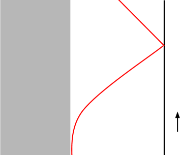
Figure 13: Left panel: bulk description of the state $V(0)|\text{TFD}\rangle$. The V-particle (whose trajectory is shown in red) escapes from the black hole (shown in gray), reaches the boundary at time $t=0$, and then falls back towards the horizon. Right panel: bulk description of the state $W(-t)V(0)|\text{TFD}\rangle$ for the case where $|t|\gtrsim t_{*}$. The W-particle (whose trajectory is shown in blue) gets blue shifted and increases the black hole size as it falls into it. The V-particle fails to scape from the larger black hole, and the perturbation $V$ never forms at the boundary.

The precise form of the above OTOC can be obtained by calculating the overlap $\langle\psi_{\textrm{\tiny out}}|\psi_{\textrm{\tiny in}}\rangle$ using the Eikonal approximation [8], in which the Eikonal phase $\delta$ is proportional to the shock wave profile $\delta\sim h(t,\vec{x})$. The OTOC can be written as an integral of the phase $e^{i\delta}$ weighted by kinematical factors which are basically Fourier transforms of bulk-to-boundary propagators for the $V$ and $W$ operators.

The result for Rindler AdS₃ reads

$$\frac{\langle V(i\epsilon_{1})W(t+i\epsilon_{2})V(i\epsilon_{3})W(t+i\epsilon_{4})\rangle}{\langle V(i\epsilon_{1})V(i\epsilon_{3})\rangle\langle W(i\epsilon_{2})W(i\epsilon_{4})\rangle}=\left(\frac{1}{1-\frac{8\pi iG_{\textrm{\tiny N}}\Delta_{W}}{\epsilon_{13}\epsilon^{*}_{24}}e^{\frac{2\pi}{\beta}\left(t-\frac{|\vec{x}|}{v_{B}}\right)}}\right)^{\Delta_{V}}$$ (44)

where $\Delta_{V}$ and $\Delta_{W}$ are the scaling dimensions of the operator $V$ and $W$, respectively, and $\epsilon_{ij}=i(e^{i\epsilon_{i}}-e^{i\epsilon_{j}})$. For this system $\beta=2\pi$ and $v_{B}=1$. This formula matches the direct CFT calculation obtained in [20]. It can also be derived using the geodesic approximation for two-sided correlators in a shock wave background [5, 20].

Expanding the above result for small values of $G_{\textrm{\tiny N}}\,e^{\frac{2\pi}{\beta}\left(t-\frac{|\vec{x}|}{v_{B}}\right)}$ we obtain

$$\text{OTO}(t)=1-8\pi iG_{\textrm{\tiny N}}\frac{\Delta_{V}\Delta_{W}}{\epsilon_{13}\epsilon^{*}_{24}}e^{\frac{2\pi}{\beta}\left(t-\frac{|\vec{x}|}{v_{B}}\right)}\,,$$ (45)

Since $h(t,\vec{x})\sim G_{\textrm{\tiny N}}\,e^{\frac{2\pi}{\beta}\left(t-\frac{|\vec{x}|}{v_{B}}\right)}$, the above result implies

$$C(t,\vec{x})\sim h(t,\vec{x}).$$ (46)

The above result is valid for small values of $G_{\textrm{\tiny N}}$, or for any value of $G_{\textrm{\tiny N}}$, but for times in the range $t_{d}<<t<<t_{*}$, where $t_{*}=\frac{\beta}{2\pi}\log\frac{1}{G_{\textrm{\tiny N}}}$.

Despite being true in the Rindler AdS₃ case, the proportionality between the double commutator and the shock wave profile has not been demonstrated in more general cases. However, the authors of [8] argued that, in regions of moderate scattering between the V- and W-particle, the identification $C(t,\vec{x})\sim h(t,\vec{x})$ is approximately valid.

At very late times, the behavior of the OTO$(t)$ is expected to be controlled by the black hole quasi-normal modes. Indeed, in the case of a compact space, it is possible to show that

$$C(t)\sim e^{-2i\omega\left(t-t_{*}-R/v_{B}\right)}\,,\,\,\text{with}\,\,\text{Im}(\omega)<0\,,$$ (47)

where $R$ is the diameter of the compact space and $\omega$ is the system lowest quasi-normal frequency [8].

4.2.1 Stringy corrections

In this section, we briefly discuss the effects of stringy corrections to the Einstein gravity results for OTOCs. We start by reviewing the Einstein gravity results from the perspective of scattering amplitudes. In the framework of the Eikonal approximation, the phase shift suffered by the V-particle is given by

$$\delta=-P^{V}h(t,\vec{x})\sim G_{\textrm{\tiny N}}\,s\,,$$ (48)

where we used the fact that $h(t,\vec{x})\sim G_{\textrm{\tiny N}}\,P^{U}$ and introduced a Mandelstam-like variable $s=2A(0)P^{U}P^{V}$. In a small-$G_{\textrm{\tiny N}}$ expansion the double commutator $C(t)$ and the phase shift $\delta$ scale with $s$ in the same way, namely

$$C(t)\sim G_{\textrm{\tiny N}}s\,,$$ (49)

where $s\sim\beta^{-2}e^{\frac{2\pi}{\beta}t}$.

The string corrections can be incorporated using the standard Veneziano formula for the relativistic scattering amplitude $\mathcal{A}\sim s\,\delta$. The phase shift can then be schematically written as an infinite sum

$$\delta\sim\sum_{J}G_{\textrm{\tiny N}}s^{J-1}\,,$$ (50)

where each term correspond to the contribution due to the exchange of a spin-$J$ field. In Einstein gravity the dominant contribution comes from the exchange of a spin-2 field, the graviton. In string theory, we have to include an infinite tower of higher spin fields. Naively, it looks like these higher spin contributions will increase the development of chaos. However, the re-summation of the above sum actually leads to a decrease in the development of chaos. The string-corrected phase shift has a milder dependence with $s$, namely

$$\delta\sim G_{\textrm{\tiny N}}s^{J_{\textrm{\tiny eff}}-1}\,,$$ (51)

with the effective spin given by [8]

$$J_{\textrm{\tiny eff}}=2-\frac{d(d-1)\ell_{s}^{2}}{4\ell_{AdS}^{2}}\,$$ (52)

where $\ell_{s}$ is the string length, $\ell_{AdS}$ is the AdS length scale and $d$ is the number of dimensions of the boundary theory. As a result, the string-corrected double commutator grows in time with an effective smaller Lyapunov exponent

$$C_{\textrm{\tiny string}}(t)\sim\,e^{\frac{2\pi}{\beta}\left(1-\frac{d(d-1)\ell_{s}^{2}}{4\ell_{AdS}^{2}}\right)t}\,,$$ (53)

and this leads to a larger scrambling time

$$t^{\textrm{\tiny string}}_{*}=t_{*}\left(1+\frac{d(d-1)\ell_{s}^{2}}{4\ell_{AdS}^{2}}\right)\,.$$ (54)

The above discussion implies that for a theory with a finite number of high-spin fields ($J>2$) chaos would develop faster than in Einstein gravity. These theories, however, are known to violate causality [54]. It is then natural to speculate that the Lyapunov exponent obtained in Einstein gravity has the maximal possible value allowed by causality. This is indeed true and this is the topic of the next section.

4.2.2 Bounds on chaos

One of the remarkable insights that came from the holographic description of quantum chaos is the fact that there is a bound on chaos - the quantum Lyapunov exponent is bounded from above, while the scrambling time is bounded from below. A distinct feature of holographic systems is that they saturate these two bounds.

Let us follow the historical order and start by discussing the lower bound on the scrambling time. In black holes physics, the scrambling time defines how fast the information that has fallen into a black hole can be recovered from the emitted Hawking radiation. In the context of the Hayden-Preskill thought experiment, the scrambling time is barely compatible with black hole complementarity [52], since a smaller scrambling time would lead to a violation of the non-clonning principle. This led Susskind and Sekino to conjecture that black holes are the fastest scramblers in nature, i.e., they have the smallest possible scrambling time [53]. The lower bound on the scrambling time of a generic many-body quantum system can be written as

$$t_{*}\geq C(\beta)\log N_{\textrm{dof}}$$ (55)

where $C(\beta)$ is some function of the inverse temperature. In the case of black holes this function is simply given by $C(\beta)=\frac{\beta}{2\pi}$.

The scrambling time defines a stronger notion of thermalization, and should not be confused with the dissipation time. In fact, for black holes, one expects the dissipation time to be given by the black hole quasinormal modes $t_{d}\sim\beta$, while the scrambling time is parametrically larger $t_{*}\sim\beta\log N_{\textrm{dof}}$. This bring us to the second bound on chaos: for systems with such a large hierarchy between the scrambling and the dissipation time is possible to derive an upper bound for the Lyapunov exponent [44]

$$\lambda_{L}\leq\frac{2\pi}{\beta}\,.$$ (56)

One should emphasize that this bound does not depend on the existence of a holographic dual. It can be derived for generic many-body quantum systems under some very reasonable assumptions.

The fact that black holes always have a maximum Lyapunov exponent led to the speculation that the saturation of the chaos bound might be a sufficient condition for a system to have an Einstein gravity dual [44, 9]. In fact, there have been many attempts to use the saturation of the chaos bound as a criterion to discriminate holographic CFTs from the non-holographic ones [20, 45, 46, 47, 48, 49, 55, 56]. It was recently shown, however, that this criterion, though necessary, is insufficient to guarantee a dual description purely in terms of Einstein gravity [57, 58].

Since $v_{B}$ defines the speed at which information propagates it is natural to question whether this quantity is also bounded. From the perspective of the boundary theory, causality implies

$$v_{B}\leq 1\,,$$ (57)

meaning that information should not propagate faster than the speed of light. Indeed, the above bound can be derived in the context of Einstein gravity by using Null Energy Condition (NEC) and assuming an asymptotically AdS geometry [59]. This is consistent with the expectation that gravity theories in asymptotically AdS geometries are dual to relativistic theories. In contrast, for geometries which are not asymptotically AdS, the butterfly velocity can surpass the speed of light [59, 42], which is consistent with the non-Lorentz invariance of the corresponding boundary theories.

If we further assume isotropy, it is possible to derive a stronger bound for $v_{B}$ [60]

$$v_{B}\leq v_{B}^{\textrm{Sch}}=\sqrt{\frac{d}{2(d-1)}}\,,$$ (58)

where $v_{B}^{\textrm{Sch}}$ is the value of the butterfly velocity for an AdS-Schwarzschild black brane in $d+1$ dimensions. This is also the butterfly velocity for a $d$-dimensional thermal CFT.

The above formula shows that, for thermal CFTs, $v_{B}$ does not depend on the temperature. However, if we deform the CFT, $v_{B}$ acquires a temperature dependence as we move along the corresponding renormalization group (RG) flow. In fact, by considering deformations that break the rotational symmetry it was noticed that the butterfly velocity violates the above bound, but remains bounded from above by its value at the infra-red (IR) fixed point, never surpassing the speed of light [61, 62, 63]. The above bound can also be violated by higher curvature corrections, but $v_{B}$ remains bounded by the speed of light as long as causality is respected. The violation of the bound given in (58) by anisotropy or higher curvature corrections is reminiscent of the well-known violation of the shear viscosity to entropy density ratio bound [66, 67, 68, 69, 70, 71].

4.3 Chaos and Entanglement Spreading

The thermofield double state displays a very atypical left-right pattern of entanglement that results from non-zero correlations between subsystems of QFT_L and QFT_R at $t=0$. The chaotic nature of the boundary theories is manifest by the fact that small perturbations added to the system in the asymptotic past destroy this delicate correlations [5].

The special pattern of entanglement can be efficiently diagnosed by considering the mutual information $I(A,B)$ between spatial subsystems $A\subset$ QFT_L and $B\subset$ QFT_R, defined as

$$I(A,B)=S_{A}+S_{B}-S_{A\cup B}\,,$$ (59)

where $S_{A}$ is the entanglement entropy of the subsystem $A$, and so on. The mutual information is always positive and provides an upper bound for correlations between operators $\mathcal{O}_{L}$ and $\mathcal{O}_{R}$ defined on $A$ and $B$, respectively [72]

$$I(A,B)\geq\frac{\left(\langle\mathcal{O}_{L}\mathcal{O}_{R}\rangle-\langle\mathcal{O}_{L}\rangle\langle\mathcal{O}_{R}\rangle\right)^{2}}{2\langle\mathcal{O}_{L}^{2}\rangle\langle\mathcal{O}_{R}^{2}\rangle}\,.$$ (60)

The thermofield double state has non-zero mutual information between large subsystems of the left and right boundary, signaling the existence of left-right correlations. These correlations can be destroyed by small perturbations in the asymptotic past, meaning that an initially positive mutual information drops to zero when we add a very early perturbation to the system.

Interestingly, the vanishing of the mutual information can be connected to the vanishing of the OTOCs discussed earlier. If, for simplicity, we assume that $\mathcal{O}_{L}$ and $\mathcal{O}_{R}$ have zero thermal one point function, then the disruption of the mutual information implies the vanishing of the following four-point function

$$\langle\mathcal{O}_{L}\mathcal{O}_{R}\rangle_{W}=\langle\textrm{TFD}|W_{R}^{\dagger}\mathcal{O}_{L}\mathcal{O}_{R}W_{R}|\textrm{TFD}\rangle=0\,,$$ (61)

which is related by analytic continuation to the one-sided out-of-time-order correlator introduced earlier.

The disruption of the mutual information has a very simple geometrical realization in the bulk. The entanglement entropies that appear in the definition of $I(A,B)$ can be holographically calculated using the HRRT prescription [73, 74]

$$S_{A}=\frac{\textrm{Area}(\gamma_{A})}{4G_{N}}\,,$$ (62)

where $\gamma_{A}$ is an extremal surface whose boundary coincides with the boundary of the region $A$. There is an analogous formula for $S_{B}$. Both $\gamma_{A}$ and $\gamma_{B}$ are U-shaped surfaces lying outside of the event horizon, in the left and right side of the geometry, respectively. There are two candidates for the extremal surface that computes $S_{A\cup B}$: the surface $\gamma_{A}\cup\gamma_{B}$, or the surface $\gamma_{\textrm{\tiny wormhole}}$ that connects the two asymptotic boundaries of the geometry. See figure 14. According to the RT prescription, we should pick the surface with less area. If $\gamma_{A}\cup\gamma_{B}$ has less area than $\gamma_{\textrm{\tiny wormhole}}$, then $I(A,B)=0$, because Area($\gamma_{A}\cup\gamma_{B}$)=Area($\gamma_{A}$)+Area($\gamma_{B}$). On the other hand, if $\gamma_{\textrm{\tiny wormhole}}$ has less area than $\gamma_{A}\cup\gamma_{B}$, i.e., Area($\gamma_{\textrm{\tiny wormhole}}$) $<$ Area($\gamma_{A}$)+Area($\gamma_{B}$), then we have a positive mutual information

$$I(A,B)=\frac{1}{4\,G_{\textrm{\tiny N}}}\left[\text{Area}(\gamma_{A})+\text{Area}(\gamma_{B})-\text{Area}(\gamma_{\textrm{\tiny wormhole}})\right]>0\,.$$ (63)

Now, an early perturbation of the thermofield double state gives rise to a shock wave geometry in which the wormhole becomes longer. As a consequence the area of the surface $\gamma_{\textrm{\tiny wormhole}}$ increases, resulting in a smaller mutual information. It is then clear that the mutual information will drop to zero if the wormhole is long enough. The length of the wormhole depends on the strength of the shock wave, which, by its turn, depends on how early is the perturbation producing it. Therefore, an early enough perturbation will produce a very long wormhole in which the mutual information will be zero. The fact that the shock wave geometry produces a longer wormhole (along the $t=0$ slice of the geometry) is clearly seen if we represent the shock wave geometry with a tilted Penrose diagram. See, for instance, the figure 3 of [75].

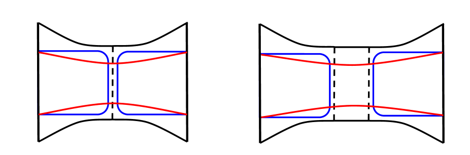
Figure 14: Illustration of the entangling surfaces in the $t=0$ slice of a two-sided black brane geometry. The U-shaped surfaces ($\gamma_{A}$ and $\gamma_{B}$) are represented by blue curves. The surface stretching through the wormhole is given by the union of the two red surfaces $\gamma_{\textrm{wormhole}}=\gamma_{1}\cup\gamma_{2}$. In the left panel we represent the unperturbed geometry, in which the two horizons coincide. In the right panel we represent the geometry in the presence of a shock wave added at some time $t_{0}$ in the past. In this case, the size of the wormhole is effectively larger, and the two horizons no longer coincide.

The mutual information $I(A,B)$ decreases as a function of the time $t_{0}$ at which we perturbed the system. For $t_{0}\gtrsim t_{*}$, the mutual information decreases linearly with behavior controlled by the so-called entanglement velocity $v_{E}$ [62]

$$\frac{dI(A,B)}{dt_{0}}=-\frac{dS_{A\cup B}}{dt_{0}}=-v_{E}\,s_{\textrm{\tiny th}}\,\text{Area}(A\cup B)\,,$$ (64)

where $s_{\textrm{\tiny th}}$ is the thermal entropy density and $\text{Area}(A\cup B)$ is the area of $A\cup B$ (or the volume of the boundary of this region). The two-sided black hole geometry with a shock wave can be thought of as an additional example of a holographic quench protocol [62], and the time-dependence of entanglement entropy can be understood in terms of the so-called ‘entanglement tsunami’ picture. See [83] for field theory calculations, and [84, 85, 86, 87, 88] for holographic calculations. However, it was recently shown that the entanglement tsunami picture is not very sharp. See [89] for further details. In [87, 88], the entanglement velocity was conjectured to be bounded as

$$v_{E}\leq v_{E}^{\textrm{\tiny Sch}}=\frac{\sqrt{d}(d-1)^{\frac{1}{2}-\frac{1}{d}}}{\left[2(d-1)\right]^{1-\frac{1}{d}}}\,,$$ (65)

where $v_{E}^{\textrm{\tiny Sch}}$ is the entanglement velocity for a $(d+1)$-dimensional Schwarzschild black brane or, equivalently, the value of $v_{E}$ for a $d$-dimensional thermal CFT. This bound can be derived in the context of Einstein gravity assuming: an asymptotically AdS geometry, isotropy and NEC [60]. Just like in the case of $v_{B}$, the entanglement velocity in thermal CFTs does not depend on the temperature. But $v_{E}$ acquires a temperature dependence if we deform the CFT and move along the corresponding RG flow [62, 63]. In these cases, $v_{E}$ violate the above bound, but it remains bounded by its corresponding value at the IR fixed point, never surpassing the speed of light.

One can also prove that the entanglement velocity is also bounded by the speed of light. This can be done by using the positivity of the mutual information [90], or using inequalities involving the relative entropy [91]. More generally, the authors of [89] conjecture that $v_{E}\leq v_{B}$, which implies the bound $v_{E}<1$ in the cases where $v_{B}$ is bounded. However, both [90, 91] assumed that the theory is Lorentz invariant. In the case of non-Lorentz invariant theories (e.g. non-commutative gauge theories) the entanglement velocity can surpass the speed of light. This has been verified both in holography calculations [42] and in field theory calculations [92].

Finally, we mention that other concepts from information theory can also be used to diagnose chaos in holography. It has been shown, for instance, that the relative entropy is also a useful tool to diagnose chaotic behavior [95]. For a connection between chaos and computational complexity, see, for instance [96, 97].

4.4 Chaos $\&$ Hydrodynamics

Recently, there has been a growing interest in the connection between chaos and hydrodynamics [98, 99, 100, 101, 102, 103, 104, 105, 106]. Here we briefly review some interesting connection between chaos and diffusion phenomena.

A longstanding goal of quantum condensed matter physics is to have a deeper understanding of the so-called ‘strange metals’. These are strongly correlated materials that do not have a description in terms of quasiparticles excitations and whose transport properties display a remarkable degree of universality. In [107, 108] Sachdev and Damle proposed that such a universal behavior could be explained by a fundamental dissipative timescale

$$\tau_{P}\sim\frac{\hbar}{2\pi k_{B}T}\,,$$ (66)

that would govern the transport in such systems.

Interestingly, the Lyapunov exponent defines a time scale $\tau_{L}=1/\lambda_{L}$, and the upper bound on $\lambda_{L}$ translates into a lower bound for $\tau_{L}$ that precisely coincides with $\tau_{P}$

$$\tau_{L}\geq\frac{\hbar\beta}{2\pi k_{B}}\,,$$ (67)

where we reintroduced $\hbar$ and the Boltzmann constant in the expression for the bound on the Lyapunov exponent. Holographic systems saturate the above bound, and this explains the universality observed in the transport properties of these systems.

A prototypical example of universality is the linear resistivity of strange metals. In [109], Hartnoll proposed that the linear resistivity could be explained by the existence of a universal lower bound on the diffusion constants related to the collective diffusion of charge and energy

$$D\gtrsim\hbar v^{2}/(k_{B}T)\,,$$ (68)

where $v$ is some characteristic velocity of the system. As $D$ is inversely proportional to the resistivity, systems saturating the above bound would display linear resistivity behavior.

One should think of (68) as a reformulation of the Kovtun-Son-Starinets (KSS) bound [111]

$$\frac{\eta}{s}\geq\frac{1}{4\pi}\frac{\hbar}{k_{B}}\,,$$ (69)

which also relies on the idea of a fundamental dissipative timescale $\tau_{L}\sim\hbar/(k_{B}T)$ controlling transport in strongly interacting systems. Naively, the observed violations of the KSS bound would seem to indicate the existence of systems in which the bound (67) is violated. The bound (68) saves the idea of a fundamental dissipative timescale by introducing an additional parameter in the game, namely, the characteristic velocity $v$. The fact that $\eta/s$ can be made arbitrarily small in some systems corresponds to the fact that the characteristic velocity is highly suppressed in those cases. See[98] for further details.

In [98, 99] Blake proposed that, at least for holographic systems with particle-hole symmetry, the characteristic velocity $v$ should be replaced by the butterfly velocity. More precisely

$$D_{c}\geq C_{c}v_{B}^{2}\tau_{L},$$ (70)

where $D_{c}$ is the electric diffusity and $C_{c}$ is a constant that depends on the universality class of theory. This proposal was motivated by the fact that both $D_{c}$ and $v_{B}$ are determined by the dynamics close to the black hole horizon in the aforementioned systems. Despite working well for systems where energy and charge diffuse independently, this proposal was shown to fail in more general cases [112, 113, 114, 115, 116]. This is related to the fact that, in more general cases, the diffusion of energy and charge is coupled, and the corresponding transport coefficients are not given only in terms of the geometry close to the black hole horizon. Hence, there is no reason for these coefficients to be related to the butterfly velocity, which is always determined solely by the near-horizon geometry.

There is, however, a universal piece of the diffusivity matrix that can be related to the chaos parameters at infra-red fixed points. This is the thermal diffusion constant [117]

$$D_{T}\geq C_{T}v_{B}^{2}\tau_{L}\,,$$ (71)

where $C_{T}$ is a universality constant (different from $C_{c}$). This proposal was shown to be valid even for systems with spatial anisotropy [118]. The above relation is not well defined when the system’s dynamical critical exponent $z$ is equal to one, but it can be extended this case [119].

Finally, we mention that there is an interesting relation between chaos and hydrodynamics that manifest itself in the so-called ‘pole-skipping’ phenomenon. See [102, 103, 104] for further details.

5 Closing remarks

The holographic description of quantum chaos not only has provided new insights into the inner-workings of gauge-gravity duality, but it has also given insights outside the scope of holography: some examples include the characterization of chaos with OTOCs, the definition of a quantum Lyapunov exponent and the existence of a bound for chaos.

The success of this new approach to quantum chaos explains the growing experimental interest that OTOCs have been received. Indeed, several protocols for measuring OTOCs have been proposed, and there are already a few experimental results. See [120] and references therein.

Finally, one of the remarkable features of quantum chaos is level statistics described by random matrices. The fact that this is present in the infrared limit of the SYK model [121, 122, 123] suggests that it should also be present in quantum black holes, although this has not yet been verified [124].

Conflicts of Interest

The author declares that there is no conflict of interest regarding the publication of this paper.

References

- [1] D. Ullmo, S. Tomsovic, “Introduction to quantum chaos”, http://www.lptms.u-psud.fr/membres/ullmo/Articles/eolss-ullmo-tomsovic.pdf, (2014)
- [2] J. M. Maldacena, “The large limit of superconformal field theories and supergravity,” Adv. Theor. Math. Phys. 2, 231 (1998) [Int. J. Theor. Phys. 38, 1113 (1999)] [hep-th/9711200].
- [3] S. S. Gubser, I. R. Klebanov, A. M. Polyakov, “Gauge theory correlators from noncritical string theory,” Phys. Lett. B428, 105-114 (1998) [hep-th/9802109].
- [4] E. Witten, “Anti-de Sitter space and holography,” Adv. Theor. Math. Phys. 2, 253-291 (1998) [hep-th/9802150].
- [5] S. H. Shenker and D. Stanford, “Black holes and the butterfly effect,” JHEP 1403, 067 (2014) [arXiv:1306.0622 [hep-th]].
- [6] S. H. Shenker and D. Stanford, “Multiple Shocks,” JHEP 1412, 046 (2014) [arXiv:1312.3296 [hep-th]].
- [7] D. A. Roberts, D. Stanford and L. Susskind, “Localized shocks,” JHEP 1503, 051 (2015) [arXiv:1409.8180 [hep-th]].
- [8] S. H. Shenker and D. Stanford, “Stringy effects in scrambling,” JHEP 1505, 132 (2015) [arXiv:1412.6087 [hep-th]].
- [9] A. Kitaev, “Hidden Correlations in the Hawking Radiation and Thermal Noise,” talk given at Fundamental Physics Prize Symposium, Nov. 10, 2014. Stanford SITP seminars, Nov. 11 and Dec. 18, 2014.
- [10] E. B. Rozenbaum, S. Ganeshan and V. Galitski, “Lyapunov Exponent and Out-of-Time-Ordered Correlator’s Growth Rate in a Chaotic System”, Phys. Rev. Lett. 188, 086801, 2017.
- [11] E. B. Rozenbaum, S. Ganeshan and V. Galitski, “Universal Level Statistics of the Out-of-Time-Ordered Operator”, arXiv:1801.10591 [cond-mat.dis-nn].
- [12] J. Chávez-Carlos, B. López-Del-Carpio, M. A. Bastarrachea-Magnani, P. Stránský, S. Lerma-Hernández, L. F. Santos and J. G. Hirsch, “Quantum and Classical Lyapunov Exponents in Atom-Field Interaction Systems,” arXiv:1807.10292 [cond-mat.stat-mech].
- [13] J. Polchinski and V. Rosenhaus, “The Spectrum in the Sachdev-Ye-Kitaev Model,” JHEP 1604, 001 (2016) doi:10.1007/JHEP04(2016)001 [arXiv:1601.06768 [hep-th]].
- [14] J. Maldacena and D. Stanford, “Remarks on the Sachdev-Ye-Kitaev model,” Phys. Rev. D 94, no. 10, 106002 (2016) doi:10.1103/PhysRevD.94.106002 [arXiv:1604.07818 [hep-th]].
- [15] J. Maldacena, D. Stanford and Z. Yang, “Conformal symmetry and its breaking in two dimensional Nearly Anti-de-Sitter space,” PTEP 2016, no. 12, 12C104 (2016) doi:10.1093/ptep/ptw124 [arXiv:1606.01857 [hep-th]].
- [16] A. Kitaev and S. J. Suh, “The soft mode in the Sachdev-Ye-Kitaev model and its gravity dual,” JHEP 1805, 183 (2018) doi:10.1007/JHEP05(2018)183 [arXiv:1711.08467 [hep-th]].
- [17] M. Axenides, E. G. Floratos and S. Nicolis, “Modular discretization of the AdS2/CFT1 holography,” JHEP 1402, 109 (2014) doi:10.1007/JHEP02(2014)109 [arXiv:1306.5670 [hep-th]].
- [18] M. Axenides, E. Floratos and S. Nicolis, “Chaotic Information Processing by Extremal Black Holes,” Int. J. Mod. Phys. D 24, no. 09, 1542012 (2015) doi:10.1142/S0218271815420122 [arXiv:1504.00483 [hep-th]].
- [19] M. Axenides, E. Floratos and S. Nicolis, “The quantum cat map on the modular discretization of extremal black hole horizons,” Eur. Phys. J. C 78, no. 5, 412 (2018) doi:10.1140/epjc/s10052-018-5850-9 [arXiv:1608.07845 [hep-th]].
- [20] D. A. Roberts and D. Stanford, “Two-dimensional conformal field theory and the butterfly effect,” Phys. Rev. Lett. 115, no. 13, 131603 (2015) [arXiv:1412.5123 [hep-th]].
- [21] D. Stanford, “Many-body chaos at weak coupling,” JHEP 1610, 009 (2016) doi:10.1007/JHEP10(2016)009 [arXiv:1512.07687 [hep-th]].
- [22] E. Plamadeala and E. Fradkin, “Scrambling in the quantum Lifshitz model,” J. Stat. Mech. 1806, no. 6, 063102 (2018). doi:10.1088/1742-5468/aac136
- [23] A. Nahum, S. Vijay and J. Haah, “Operator Spreading in Random Unitary Circuits,” Phys. Rev. X 8, no. 2, 021014 (2018) doi:10.1103/PhysRevX.8.021014 [arXiv:1705.08975 [cond-mat.str-el]].
- [24] V. Khemani, A. Vishwanath and D. A. Huse, “Operator spreading and the emergence of dissipation in unitary dynamics with conservation laws,” Phys. Rev. X 8, no. 3, 031057 (2018) doi:10.1103/PhysRevX.8.031057 [arXiv:1710.09835 [cond-mat.stat-mech]].
- [25] T. Rakovszky, F. Pollmann and C. W. von Keyserlingk, “Diffusive hydrodynamics of out-of-time-ordered correlators with charge conservation,” Phys. Rev. X 8, no. 3, 031058 (2018) doi:10.1103/PhysRevX.8.031058 [arXiv:1710.09827 [cond-mat.stat-mech]].
- [26] D. J. Luitz and Y. Bar Lev, “Information propagation in isolated quantum systems,” Phys. Rev. B 96, no. 2, 020406 (2017) doi:10.1103/PhysRevB.96.020406 [arXiv:1702.03929 [cond-mat.dis-nn]].
- [27] A. Bohrdt, C. B. Mendl, M. Endres and M. Knap, “Scrambling and thermalization in a diffusive quantum many-body system,” New J. Phys. 19, no. 6, 063001 (2017) doi:10.1088/1367-2630/aa719b [arXiv:1612.02434 [cond-mat.quant-gas]].
- [28] M. Heyl, F. Pollman, and B. Dóra, “Detecting Equilibrium and Dynamical Quantum Phase Transitions in Ising Chains via Out-of-Time-Ordered Correlators,” Phys. Rev. Lett. 121, 016801 (2018) doi:10.1103/PhysRevLett.121.016801
- [29] C-J. Lin, O. I. Motrunich, “Out-of-time-ordered correlators in quantum Ising chain,” Phys. Rev. B 97, 144304 (2018) doi:10.1103/PhysRevB.97.144304
- [30] S. Xu and B. Swingle, “Accessing scrambling using matrix product operators,” arXiv:1802.00801 [quant-ph].
- [31] M. Cencini, F. Cecconi and A. Vulpiani, “Chaos: From Simple Models to Complex Systems,” World Scientific: Singapore, 2009.
- [32] J. Polchinski, “Chaos in the black hole S-matrix,” arXiv:1505.08108 [hep-th].
- [33] I. García-Mata, M. Saraceno, R. A. Jalabert, A. J. Roncaglia and D. A. Wisniacki, “Chaos signatures in the short and long time behavior of the out-of-time ordered correlator,” Phys. Rev. Lett. 121, no. 21, 210601 (2018) doi:10.1103/PhysRevLett.121.210601 [arXiv:1806.04281 [quant-ph]].
- [34] D. Stanford, “Many-body quantum chaos,” Seminar at the school IAS PiTP 2018: From Qubtis to Spacetime. https://video.ias.edu/PiTP/2018/0723-DouglasStanford
- [35] A. I. Larkin and Y. N. Ovchinnikov, “Quasiclassical method in the theory of superconductivity,” JETP 28, 6 (1969), 1200-1205.
- [36] V. Khemani, D. A. Huse and A. Nahum, “Velocity-dependent Lyapunov exponents in many-body quantum, semiclassical, and classical chaos,” Phys. Rev. B 98, no. 14, 144304 (2018) doi:10.1103/PhysRevB.98.144304 [arXiv:1803.05902 [cond-mat.stat-mech]].
- [37] D. A. Roberts and B. Swingle, “Lieb-Robinson Bound and the Butterfly Effect in Quantum Field Theories,” Phys. Rev. Lett. 117, no. 9, 091602 (2016) [arXiv:1603.09298 [hep-th]].
- [38] J. M. Maldacena, “Eternal black holes in anti-de Sitter,” JHEP 0304, 021 (2003) [hep-th/0106112].
- [39] L. Fidkowski, V. Hubeny, M. Kleban and S. Shenker, “The Black hole singularity in AdS / CFT,” JHEP 0402, 014 (2004) doi:10.1088/1126-6708/2004/02/014 [hep-th/0306170].
- [40] T. Dray and G. ’t Hooft, “The Gravitational Shock Wave of a Massless Particle,” Nucl. Phys. B 253, 173 (1985).
- [41] K. Sfetsos, “On gravitational shock waves in curved space-times,” Nucl. Phys. B 436, 721 (1995) [hep-th/9408169].
- [42] W. Fischler, V. Jahnke and J. F. Pedraza, “Chaos and entanglement spreading in a non-commutative gauge theory,” JHEP 1811, 072 (2018) doi:10.1007/JHEP11(2018)072 [arXiv:1808.10050 [hep-th]].
- [43] M. Baggioli, B. Padhi, P. W. Phillips and C. Setty, “Conjecture on the Butterfly Velocity across a Quantum Phase Transition,” JHEP 1807, 049 (2018) doi:10.1007/JHEP07(2018)049 [arXiv:1805.01470 [hep-th]].
- [44] J. Maldacena, S. H. Shenker and D. Stanford, “A bound on chaos,” JHEP 1608, 106 (2016) [arXiv:1503.01409 [hep-th]].
- [45] E. Perlmutter, “Bounding the Space of Holographic CFTs with Chaos,” JHEP 1610, 069 (2016) [arXiv:1602.08272 [hep-th]].
- [46] A. L. Fitzpatrick and J. Kaplan, “A Quantum Correction To Chaos,” JHEP 1605, 070 (2016) [arXiv:1601.06164 [hep-th]].
- [47] P. Caputa, T. Numasawa and A. Veliz-Osorio, “Out-of-time-ordered correlators and purity in rational conformal field theories,” PTEP 2016, no. 11, 113B06 (2016) [arXiv:1602.06542 [hep-th]].
- [48] G. Turiaci and H. Verlinde, “On CFT and Quantum Chaos,” JHEP 1612, 110 (2016) [arXiv:1603.03020 [hep-th]].
- [49] P. Caputa, Y. Kusuki, T. Takayanagi and K. Watanabe, “Out-of-Time-Ordered Correlators in ,” Phys. Rev. D 96, no. 4, 046020 (2017) [arXiv:1703.09939 [hep-th]].
- [50] M. Taylor, “Generalized conformal structure, dilaton gravity and SYK,” JHEP 1801, 010 (2018) doi:10.1007/JHEP01(2018)010 [arXiv:1706.07812 [hep-th]].
- [51] S. Grozdanov, “On the connection between hydrodynamics and quantum chaos in holographic theories with stringy corrections,” arXiv:1811.09641 [hep-th].
- [52] P. Hayden and J. Preskill, “Black holes as mirrors: Quantum information in random subsystems,” JHEP 0709, 120 (2007) [arXiv:0708.4025 [hep-th]].
- [53] Y. Sekino and L. Susskind, “Fast Scramblers,” JHEP 0810, 065 (2008) [arXiv:0808.2096 [hep-th]].
- [54] X. O. Camanho, J. D. Edelstein, J. Maldacena and A. Zhiboedov, “Causality Constraints on Corrections to the Graviton Three-Point Coupling,” JHEP 1602, 020 (2016) [arXiv:1407.5597 [hep-th]].
- [55] B. Michel, J. Polchinski, V. Rosenhaus and S. J. Suh, “Four-point function in the IOP matrix model,” JHEP 1605, 048 (2016) [arXiv:1602.06422 [hep-th]].
- [56] P. Padmanabhan, S. J. Rey, D. Teixeira and D. Trancanelli, “Supersymmetric many-body systems from partial symmetries — integrability, localization and scrambling,” JHEP 1705, 136 (2017) doi:10.1007/JHEP05(2017)136 [arXiv:1702.02091 [hep-th]].
- [57] J. de Boer, E. Llabrés, J. F. Pedraza and D. Vegh, “Chaotic strings in AdS/CFT,” Phys. Rev. Lett. 120, no. 20, 201604 (2018) [arXiv:1709.01052 [hep-th]].
- [58] A. Banerjee, A. Kundu and R. R. Poojary, “Strings, Branes, Schwarzian Action and Maximal Chaos,” arXiv:1809.02090 [hep-th].
- [59] X. L. Qi and Z. Yang, “Butterfly velocity and bulk causal structure,” arXiv:1705.01728 [hep-th].
- [60] M. Mezei, “On entanglement spreading from holography,” JHEP 1705, 064 (2017) [arXiv:1612.00082 [hep-th]].
- [61] D. Giataganas, U. Gürsoy and J. F. Pedraza, “Strongly-coupled anisotropic gauge theories and holography,” arXiv:1708.05691 [hep-th].
- [62] V. Jahnke, “Delocalizing entanglement of anisotropic black branes,” JHEP 1801, 102 (2018) [arXiv:1708.07243 [hep-th]].
- [63] D. Avila, V. Jahnke and L. Patiño, “Chaos, Diffusivity, and Spreading of Entanglement in Magnetic Branes, and the Strengthening of the Internal Interaction,” JHEP 1809, 131 (2018) doi:10.1007/JHEP09(2018)131 [arXiv:1805.05351 [hep-th]].
- [64] X. O. Camanho and J. D. Edelstein, “Causality constraints in AdS/CFT from conformal collider physics and Gauss-Bonnet gravity,” JHEP 1004, 007 (2010) [arXiv:0911.3160 [hep-th]].
- [65] A. Buchel, J. Escobedo, R. C. Myers, M. F. Paulos, A. Sinha and M. Smolkin, “Holographic GB gravity in arbitrary dimensions,” JHEP 1003, 111 (2010) [arXiv:0911.4257 [hep-th]].
- [66] M. Brigante, H. Liu, R. C. Myers, S. Shenker and S. Yaida, “Viscosity Bound Violation in Higher Derivative Gravity,” Phys. Rev. D 77, 126006 (2008) [arXiv:0712.0805 [hep-th]].
- [67] M. Brigante, H. Liu, R. C. Myers, S. Shenker and S. Yaida, “The Viscosity Bound and Causality Violation,” Phys. Rev. Lett. 100, 191601 (2008) [arXiv:0802.3318 [hep-th]].
- [68] X. O. Camanho, J. D. Edelstein and M. F. Paulos, “Lovelock theories, holography and the fate of the viscosity bound,” JHEP 1105, 127 (2011) [arXiv:1010.1682 [hep-th]].
- [69] J. Erdmenger, P. Kerner and H. Zeller, “Non-universal shear viscosity from Einstein gravity,” Phys. Lett. B 699, 301 (2011) [arXiv:1011.5912 [hep-th]].
- [70] A. Rebhan and D. Steineder, “Violation of the Holographic Viscosity Bound in a Strongly Coupled Anisotropic Plasma,” Phys. Rev. Lett. 108, 021601 (2012) [arXiv:1110.6825 [hep-th]].
- [71] V. Jahnke, A. S. Misobuchi and D. Trancanelli, “Holographic renormalization and anisotropic black branes in higher curvature gravity,” JHEP 1501, 122 (2015) [arXiv:1411.5964 [hep-th]].
- [72] M. M. Wolf, F. Verstraete, M. B. Hastings, and J. I. Cirac, “Area laws in quantum systems: Mutual information and correlations”, Phys. Rev. Lett. 100, 070502 (2008) [arXiv:0704.3906 [quant-ph]].
- [73] S. Ryu and T. Takayanagi, “Holographic derivation of entanglement entropy from AdS/CFT,” Phys. Rev. Lett. 96, 181602 (2006) [hep-th/0603001].
- [74] V. E. Hubeny, M. Rangamani and T. Takayanagi, “A Covariant holographic entanglement entropy proposal,” JHEP 0707, 062 (2007) [arXiv:0705.0016 [hep-th]].
- [75] S. Leichenauer, “Disrupting Entanglement of Black Holes,” Phys. Rev. D 90, no. 4, 046009 (2014) [arXiv:1405.7365 [hep-th]].
- [76] N. Sircar, J. Sonnenschein and W. Tangarife, “Extending the scope of holographic mutual information and chaotic behavior,” JHEP 1605, 091 (2016) [arXiv:1602.07307 [hep-th]].
- [77] Y. Ling, P. Liu and J. P. Wu, “Holographic Butterfly Effect at Quantum Critical Points,” JHEP 1710, 025 (2017) [arXiv:1610.02669 [hep-th]].
- [78] R. G. Cai, X. X. Zeng and H. Q. Zhang, “Influence of inhomogeneities on holographic mutual information and butterfly effect,” JHEP 1707, 082 (2017) [arXiv:1704.03989 [hep-th]].
- [79] M. M. Qaemmaqami, “Criticality in third order lovelock gravity and butterfly effect,” Eur. Phys. J. C 78, no. 1, 47 (2018) [arXiv:1705.05235 [hep-th]].
- [80] S. F. Wu, B. Wang, X. H. Ge and Y. Tian, “Holographic RG flow of thermoelectric transport with momentum dissipation,” Phys. Rev. D 97, no. 6, 066029 (2018) [arXiv:1706.00718 [hep-th]].
- [81] M. M. Qaemmaqami, “Butterfly effect in 3D gravity,” Phys. Rev. D 96, no. 10, 106012 (2017) [arXiv:1707.00509 [hep-th]].
- [82] H. S. Jeong, Y. Ahn, D. Ahn, C. Niu, W. J. Li and K. Y. Kim, “Thermal diffusivity and butterfly velocity in anisotropic Q-Lattice models,” JHEP 1801, 140 (2018) [arXiv:1708.08822 [hep-th]].
- [83] P. Calabrese and J. L. Cardy, “Evolution of entanglement entropy in one-dimensional systems,” J. Stat. Mech. 0504, P04010 (2005) [cond-mat/0503393].
- [84] J. Abajo-Arrastia, J. Aparicio and E. Lopez, “Holographic Evolution of Entanglement Entropy,” JHEP 1011, 149 (2010) [arXiv:1006.4090 [hep-th]].
- [85] T. Albash and C. V. Johnson, “Evolution of Holographic Entanglement Entropy after Thermal and Electromagnetic Quenches,” New J. Phys. 13, 045017 (2011) [arXiv:1008.3027 [hep-th]].
- [86] T. Hartman and J. Maldacena, “Time Evolution of Entanglement Entropy from Black Hole Interiors,” JHEP 1305, 014 (2013) [arXiv:1303.1080 [hep-th]].
- [87] H. Liu and S. J. Suh, “Entanglement Tsunami: Universal Scaling in Holographic Thermalization,” Phys. Rev. Lett. 112, 011601 (2014) [arXiv:1305.7244 [hep-th]].
- [88] H. Liu and S. J. Suh, “Entanglement growth during thermalization in holographic systems,” Phys. Rev. D 89, no. 6, 066012 (2014) [arXiv:1311.1200 [hep-th]].
- [89] M. Mezei and D. Stanford, “On entanglement spreading in chaotic systems,” JHEP 1705, 065 (2017) [arXiv:1608.05101 [hep-th]].
- [90] H. Casini, H. Liu and M. Mezei, “Spread of entanglement and causality,” JHEP 1607, 077 (2016) [arXiv:1509.05044 [hep-th]].
- [91] T. Hartman and N. Afkhami-Jeddi, “Speed Limits for Entanglement,” arXiv:1512.02695 [hep-th].
- [92] P. Sabella-Garnier, “Time dependence of entanglement entropy on the fuzzy sphere,” JHEP 1708, 121 (2017) [arXiv:1705.01969 [hep-th]].
- [93] S. Kundu and J. F. Pedraza, “Spread of entanglement for small subsystems in holographic CFTs,” Phys. Rev. D 95, no. 8, 086008 (2017) [arXiv:1602.05934 [hep-th]].
- [94] S. F. Lokhande, G. W. J. Oling and J. F. Pedraza, “Linear response of entanglement entropy from holography,” JHEP 1710, 104 (2017) [arXiv:1705.10324 [hep-th]].
- [95] Y. O. Nakagawa, G. Sárosi and T. Ugajin, “Chaos and relative entropy,” JHEP 1807, 002 (2018) doi:10.1007/JHEP07(2018)002 [arXiv:1805.01051 [hep-th]].
- [96] J. M. Magán, “Black holes, complexity and quantum chaos,” JHEP 1809, 043 (2018) doi:10.1007/JHEP09(2018)043 [arXiv:1805.05839 [hep-th]].
- [97] S. A. Hosseini Mansoori and M. M. Qaemmaqami, “Complexity Growth, Butterfly Velocity and Black hole Thermodynamics,” arXiv:1711.09749 [hep-th].
- [98] M. Blake, “Universal Charge Diffusion and the Butterfly Effect in Holographic Theories,” Phys. Rev. Lett. 117, no. 9, 091601 (2016) [arXiv:1603.08510 [hep-th]].
- [99] M. Blake, “Universal Diffusion in Incoherent Black Holes,” Phys. Rev. D 94, no. 8, 086014 (2016) [arXiv:1604.01754 [hep-th]].
- [100] R. A. Davison, W. Fu, A. Georges, Y. Gu, K. Jensen and S. Sachdev, “Thermoelectric transport in disordered metals without quasiparticles: The Sachdev-Ye-Kitaev models and holography,” Phys. Rev. B 95, no. 15, 155131 (2017) [arXiv:1612.00849 [cond-mat.str-el]].
- [101] M. Blake, R. A. Davison and S. Sachdev, “Thermal diffusivity and chaos in metals without quasiparticles,” Phys. Rev. D 96, no. 10, 106008 (2017) [arXiv:1705.07896 [hep-th]].
- [102] S. Grozdanov, K. Schalm and V. Scopelliti, “Black hole scrambling from hydrodynamics,” Phys. Rev. Lett. 120, no. 23, 231601 (2018) [arXiv:1710.00921 [hep-th]].
- [103] M. Blake, H. Lee and H. Liu, “A quantum hydrodynamical description for scrambling and many-body chaos,” arXiv:1801.00010 [hep-th].
- [104] S. Grozdanov, K. Schalm and V. Scopelliti, “Kinetic theory for classical and quantum many-body chaos,” arXiv:1804.09182 [hep-th].
- [105] M. Blake, R. A. Davison, S. Grozdanov and H. Liu, “Many-body chaos and energy dynamics in holography,” JHEP 1810, 035 (2018) doi:10.1007/JHEP10(2018)035 [arXiv:1809.01169 [hep-th]].
- [106] F. M. Haehl and M. Rozali, “Effective Field Theory for Chaotic CFTs,” JHEP 1810, 118 (2018) doi:10.1007/JHEP10(2018)118 [arXiv:1808.02898 [hep-th]].
- [107] S. Sachdev and K. Damle “Non-zero temperature transport near quantum critical point” Phys. Rev. B bf 56, 8714 (1997). [arXiv:cond-mat/9705206]
- [108] S. Sachdev, “Quantum phase transitions,” Cambrigde University Press (1999)
- [109] S. A. Hartnoll, “Theory of universal incoherent metallic transport,” Nature Phys. 11, 54 (2015) doi:10.1038/nphys3174 [arXiv:1405.3651 [cond-mat.str-el]].
- [110] H. S. Jeong, K. Y. Kim and C. Niu, “Linear- resistivity at high temperature,” JHEP 1810, 191 (2018) doi:10.1007/JHEP10(2018)191 [arXiv:1806.07739 [hep-th]].
- [111] P. Kovtun, D. T. Son and A. O. Starinets, “Viscosity in strongly interacting quantum field theories from black hole physics,” Phys. Rev. Lett. 94, 111601 (2005) doi:10.1103/PhysRevLett.94.111601 [hep-th/0405231].
- [112] A. Lucas and J. Steinberg, “Charge diffusion and the butterfly effect in striped holographic matter,” JHEP 1610, 143 (2016) doi:10.1007/JHEP10(2016)143 [arXiv:1608.03286 [hep-th]].
- [113] R. A. Davison, W. Fu, A. Georges, Y. Gu, K. Jensen and S. Sachdev, “Thermoelectric transport in disordered metals without quasiparticles: The Sachdev-Ye-Kitaev models and holography,” Phys. Rev. B 95, no. 15, 155131 (2017) doi:10.1103/PhysRevB.95.155131 [arXiv:1612.00849 [cond-mat.str-el]].
- [114] M. Baggioli, B. Goutéraux, E. Kiritsis and W. J. Li, “Higher derivative corrections to incoherent metallic transport in holography,” JHEP 1703, 170 (2017) doi:10.1007/JHEP03(2017)170 [arXiv:1612.05500 [hep-th]].
- [115] K. Y. Kim and C. Niu, “Diffusion and Butterfly Velocity at Finite Density,” JHEP 1706, 030 (2017) doi:10.1007/JHEP06(2017)030 [arXiv:1704.00947 [hep-th]].
- [116] A. Mokhtari, S. A. Hosseini Mansoori and K. Bitaghsir Fadafan, “Diffusivities bounds in the presence of Weyl corrections,” Phys. Lett. B 785, 591 (2018) doi:10.1016/j.physletb.2018.09.020 [arXiv:1710.03738 [hep-th]].
- [117] M. Blake, R. A. Davison and S. Sachdev, “Thermal diffusivity and chaos in metals without quasiparticles,” Phys. Rev. D 96, no. 10, 106008 (2017) doi:10.1103/PhysRevD.96.106008 [arXiv:1705.07896 [hep-th]].
- [118] D. Ahn, Y. Ahn, H. S. Jeong, K. Y. Kim, W. J. Li and C. Niu, “Thermal diffusivity and butterfly velocity in anisotropic Q-Lattice models,” arXiv:1708.08822 [hep-th].
- [119] R. A. Davison, S. A. Gentle and B. Goutéraux, “Impact of irrelevant deformations on thermodynamics and transport in holographic quantum critical states,” arXiv:1812.11060 [hep-th].
- [120] B. Swingle, “Unscrambling the physics of out-of-time-order correlators”, Nature Physics, 14, 988–990 (2018)
- [121] J. S. Cotler et al., “Black Holes and Random Matrices,” JHEP 1705, 118 (2017) Erratum: [JHEP 1809, 002 (2018)] doi:10.1007/JHEP09(2018)002, 10.1007/JHEP05(2017)118 [arXiv:1611.04650 [hep-th]].
- [122] A. M. García-García and J. J. M. Verbaarschot, “Spectral and thermodynamic properties of the Sachdev-Ye-Kitaev model,” Phys. Rev. D 94, no. 12, 126010 (2016) doi:10.1103/PhysRevD.94.126010 [arXiv:1610.03816 [hep-th]].
- [123] A. M. García-García and J. J. M. Verbaarschot, “Analytical Spectral Density of the Sachdev-Ye-Kitaev Model at finite N,” Phys. Rev. D 96, no. 6, 066012 (2017) doi:10.1103/PhysRevD.96.066012 [arXiv:1701.06593 [hep-th]].
- [124] P. Saad, S. H. Shenker and D. Stanford, “A semiclassical ramp in SYK and in gravity,” arXiv:1806.06840 [hep-th].