A Balancing Domain Decomposition by Constraints Preconditioner for a $C^{0}$ Interior Penalty Method

1 Introduction

Consider the following weak formulation of a fourth order problem on a bounded polygonal domain $\Omega$ in $\mathbb{R}^{2}$:

Find $u\in\SS$ such that

$$\int_{\Omega}\nabla^{2}u:\nabla^{2}v\,dx=\int_{\Omega}fv\,dx\qquad\forall\,v\in\SS,$$ (1)

where $f\in L_{2}(\Omega)$, and $\nabla^{2}v:\nabla^{2}w=\sum_{i,j=1}^{2}(\partial^{2}v/\partial x_{i}\partial x_{j})(\partial^{2}w/\partial x_{i}\partial x_{j})$ is the inner product of the Hessian matrices of $v$ and $w$.

For simplicity, let $\mathcal{T}_{h}$ be a quasi-uniform triangulation of $\Omega$ consisting of rectangles and take $V_{h}\subset H_{0}^{1}(\Omega)$ to be the $Q_{2}$ Lagrange finite element space associated with $\mathcal{T}_{h}$. Then the model problem (1) can be discretized by the following $C^{0}$ interior penalty Galerkin method EGHLMT:2002:C0 ; BS:2005:C0IP :

Find $u_{h}\in V_{h}$ such that

$$a_{h}(u_{h},v)=\int_{\Omega}fv\,dx\qquad v\in V_{h},$$

where

$$a_{h}(v,w) =\sum_{D\in\mathcal{T}_{h}}\int_{T}\nabla^{2}v:\nabla^{2}w\,dx+\sum_{e\in\mathcal{E}_{h}}\frac{\eta}{|e|}\int_{e}\left[\left[\frac{\partial v}{\partial\mathbf{n}}\right]\right]\left[\left[\frac{\partial w}{\partial\mathbf{n}}\right]\right]\,ds$$

$$\hskip 40.0pt+\sum_{e\in\mathcal{E}_{h}}\int_{e}\left(\left\{\left\{\frac{\partial^{2}v}{\partial\mathbf{n}^{2}}\right\}\right\}\left[\left[\frac{\partial w}{\partial\mathbf{n}}\right]\right]+\left\{\left\{\frac{\partial^{2}w}{\partial\mathbf{n}^{2}}\right\}\right\}\left[\left[\frac{\partial v}{\partial\mathbf{n}}\right]\right]\right)\,ds.$$

Here $\eta$ is a positive penalty parameter, $\mathcal{E}_{h}$ is the set of edges of $\mathcal{T}_{h}$, and $|e|$ is the length of the edge $e$. The jump $\left[\left[\cdot\right]\right]$ and the average $\left\{\left\{\cdot\right\}\right\}$ are defined as follows.

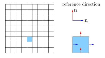
Figure 1: (a) A triangulation of $\Omega$. (b) A reference direction of normal vectors on the edges of $T\in\mathcal{T}_{h}$.

Let $\mathbf{n}_{e}$ be the unit normal chosen according to a reference direction shown in Fig. 1. If $e$ is an interior edge of $\mathcal{T}_{h}$ shared by two elements $D_{-}$ and $D_{+}$, we define on $e$,

$$\left[\left[\frac{\partial v}{\partial\mathbf{n}}\right]\right]=\frac{\partial v_{+}}{\partial\mathbf{n}_{e}}-\frac{\partial v_{-}}{\partial\mathbf{n}_{e}}\quad\text{and}\quad\left\{\left\{\frac{\partial^{2}v}{\partial\mathbf{n}^{2}}\right\}\right\}=\frac{1}{2}\left(\frac{\partial^{2}v_{+}}{\partial\mathbf{n}_{e}^{2}}+\frac{\partial^{2}v_{-}}{\partial\mathbf{n}_{e}^{2}}\right),$$

where $v_{\pm}=v|_{D_{\pm}}$. On an edge of $\mathcal{T}_{h}$ along $\partial\Omega$, we define

$$\left[\left[\frac{\partial v}{\partial\mathbf{n}}\right]\right]=\pm\frac{\partial v}{\partial\mathbf{n}_{e}}\quad\text{and}\quad\left\{\left\{\frac{\partial^{2}v}{\partial\mathbf{n}^{2}}\right\}\right\}=\frac{\partial^{2}v}{\partial\mathbf{n}_{e}^{2}},$$

in which the negative sign is chosen if $\mathbf{n}_{e}$ points towards the outside of $\Omega$, and the positive sign otherwise.

It is noted that for $\eta>0$ sufficiently large (Lemma 6 in BS:2005:C0IP ), there exist positive constants $C_{1}$ and $C_{2}$ independent of $h$ such that

$$C_{1}a_{h}(v,v)\leq|v|_{H^{2}(\Omega,{\mathcal{T}_{h}})}^{2}\leq C_{2}a_{h}(v,v)\quad\forall v\in V_{h},$$

where

$$|v|_{H^{2}(\Omega,{\mathcal{T}_{h}})}^{2}=\sum_{D\in\mathcal{T}_{h}}|v|^{2}_{H^{2}(D)}+\sum_{e\in\mathcal{E}_{h}}\frac{1}{|e|}\left\|\left[\left[\frac{\partial v}{\partial\mathbf{n}}\right]\right]\right\|^{2}_{L_{2}(e)}.$$

Compared with classical finite element methods for fourth order problems, $C^{0}$ interior penalty methods have many advantages BS:2005:C0IP ; BW:2012:BPSforC0 ; EGHLMT:2002:C0 . However, due to the nature of fourth order problems, the condition number of the discrete problem resulting from $C^{0}$ interior penalty methods grows at the rate of $h^{-4}$ LW:2007:DDM . Thus a good preconditioner is essential for solving the discrete problem efficiently and accurately. In this paper, we develop a nonoverlapping domain decomposition preconditioner for $C^{0}$ interior penalty methods that is based on the balancing domain decomposition by constraints (BDDC) approach Dohrmann:2003:BDDC ; BS:2007:BDDCFETI ; BPS:2017:SIPGBDDC .

The rest of the paper is organized as follows. In Section 2 we introduce the subspace decomposition. We then design a BDDC preconditioner for the reduced problem in Section 3, followed by condition number estimates in Section 4. Finally, we report numerical results in Section 5 that illustrate the performance of the proposed preconditioner and corroborate the theoretical estimates.

2 A Subspace Decomposition

We begin with a nonoverlapping domain decomposition of $\Omega$ consisting of rectangular (open) subdomains $\Omega_{1},\Omega_{2},\cdots,\Omega_{J}$ aligned with $\mathcal{T}_{h}$ such that $\partial\Omega_{j}\bigcap\partial\Omega_{\ell}=\emptyset,$ a vertex, or an edge, if $j\neq\ell$.

We assume the subdomains are shape regular and denote the typical diameter of the subdomains by $H$. Let $\Gamma=\left(\bigcup_{j=1}^{J}\partial\Omega_{j}\right)\backslash\partial\Omega$ be the interface of the subdomains, and $\mathcal{E}_{h,\Gamma}$ be the subset of $\mathcal{E}_{h}$ containing the edges on $\Gamma$.

Since the condition that the normal derivative of $v$ vanishes on $\Gamma$ is implicit in terms of the standard degrees of freedom (dofs) of the $Q_{2}$ finite element, it is more convenient to use the modified $Q_{2}$ finite element space (Fig. 2) as $V_{h}$. Details of the modified $Q_{2}$ finite element space can be found in BW:2012:BPSforC0 .

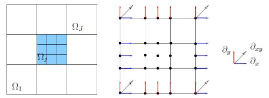
Figure 2: (a) A nonoverlapping decomposition of $\Omega$ into $\Omega_{1},\cdots,\Omega_{J}$ and a triangulation of the subdomain $\Omega_{j}$. (b) Dofs of $V_{h}|_{\Omega_{j}}$. (c) Reference directions for the first order and mixed derivatives.

First of all, we decompose $V_{h}$ into two subspaces

$$V_{h}=V_{h,C}\oplus V_{h,D},$$

where

$$V_{h,C}=\bigg{\{}v\in V_{h}:\left[\left[\frac{\partial v}{\partial\mathbf{n}}\right]\right]=0\text{ on the edges in $\mathcal{E}_{h}$ that are subsets of }\bigcup_{j=1}^{J}\partial\Omega_{j}\bigg{\}}$$

and

$$V_{h,D} =\bigg{\{}v\in V_{h}:\left\{\left\{\frac{\partial v}{\partial\mathbf{n}}\right\}\right\}=0\text{ on edges in }\mathcal{E}_{h,\Gamma},\text{ and }$$

$$\hskip 99.58464ptv\text{ vanishes at all interior nodes of each subdomain}\bigg{\}}.$$

Let $A_{h}:V_{h}\rightarrow V_{h}^{\prime}$ be the symmetric positive definite (SPD) operator defined by

$$\langle A_{h}v,w\rangle=a_{h}(v,w)\qquad\forall\,v,w\in V_{h},$$

where $\langle\cdot,\cdot\rangle$ is the canonical bilinear form between a vector space and its dual. Similarly, we define $A_{h,C}:V_{h,C}\rightarrow V_{h,C}^{\prime}$ and $A_{h,D}:V_{h,D}\rightarrow V_{h,D}^{\prime}$ by

$$\langle A_{h,C}v,w\rangle=a_{h}(v,w)\quad\forall\,v,w\in V_{h,C}\quad\text{and}\quad\langle A_{h,D}v,w\rangle=a_{h}(v,w)\quad\forall\,v,w\in V_{h,D}.$$

Then we have the following lemma.

Lemma 1

For any $v\in V_{h}$, there is a unique decomposition $v=v_{\scriptscriptstyle C}+v_{\scriptscriptstyle D}$, where $v_{\scriptscriptstyle C}\in V_{h,C}$ and $v_{\scriptscriptstyle D}\in V_{h,D}$. In addition, it holds that

$$\langle A_{h}v,v\rangle\approx\langle A_{h,C}v_{C},v_{C}\rangle+\langle A_{h,D}v_{D},v_{D}\rangle\quad\forall\,v\in V_{h}.$$

Remark 1

Since the subspace $V_{h,D}$ only contains dofs on the boundary of subdomains, the size of the matrix $A_{h,D}$ is of order $J/h$. We can implement the solve $A_{h,D}^{-1}$ directly. Therefore, it is crucial to have an efficient preconditioner for $A_{h,C}$.

Because functions in $V_{h,C}$ have continuous normal derivatives on the edges in $\mathcal{E}_{h,\Gamma}$ and vanishing normal derivatives on $\partial\Omega$, it is easy to observe that

$$a_{h}(v,w)=\sum_{j=1}^{J}a_{h,j}(v_{j},w_{j})\qquad\forall\,v,w\in V_{h,C},$$

where $v_{j}=v\big{|}_{\Omega_{j}},w_{j}=w\big{|}_{\Omega_{j}}$, and $a_{h,j}(\cdot,\cdot)$ is the analog of $a_{h}(\cdot,\cdot)$ defined on elements and interior edges of $\Omega_{j}$. Note that $a_{h,j}(\cdot,\cdot)$ is a localized bilinear form.

Next we define

$$V_{h,C}(\Omega\backslash\Gamma) =\left\{v\in V_{h,C}:v\,\,\,\mbox{has its vanishing derivatives up to order 1 on}\,\,\,\Gamma\right\}$$

$$V_{h,C}(\Gamma) =\left\{v\in V_{h,C}:a_{h}(v,w)=0,\,\,\,\forall\,w\in V_{h,C}(\Omega\backslash\Gamma)\right\}.$$

Functions in $V_{h,C}(\Gamma)$ are referred to as discrete biharmonic functions. They are uniquely determined by the dofs associated with $\Gamma$.

For any $v_{C}\in V_{h,C}$, there is a unique decomposition $v_{C}=v_{C,\Omega\backslash\Gamma}+v_{C,\Gamma}$, where $v_{C,\Omega\backslash\Gamma}\in V_{h,C}(\Omega\backslash\Gamma)$ and $v_{C,\Gamma}\in V_{h,C}(\Gamma)$. Furthermore, let $A_{h,C,\Omega\backslash\Gamma}:V_{h,C}(\Omega\backslash\Gamma)\rightarrow V_{h,C}(\Omega\backslash\Gamma)^{\prime}$ and $S_{h}:V_{h,C}(\Gamma)\rightarrow V_{h,C}(\Gamma)^{\prime}$ be SPD operators defined by

$$\langle A_{h,C,\Omega\backslash\Gamma}v,w\rangle =a_{h}(v,w)\quad\forall\,v,w\in V_{h,C}(\Omega\backslash\Gamma),$$

$$\langle S_{h}v,w\rangle =a_{h}(v,w)\quad\forall\,v,w\in V_{h,C}(\Gamma),$$

then it holds that for all $v_{\scriptscriptstyle C}\in V_{h,C}$ with $v_{\scriptscriptstyle C}={v}_{\scriptscriptstyle C,\Omega\setminus\Gamma}+{v}_{\scriptscriptstyle C,\Gamma}$,

$$\langle A_{h,C}v_{C},v_{C}\rangle=\langle A_{h,C,\Omega\backslash\Gamma}v_{C,\Omega\backslash\Gamma},v_{C,\Omega\backslash\Gamma}\rangle+\langle S_{h}v_{C,\Gamma},v_{C,\Gamma}\rangle.$$

Remark 2

It is noted that $A_{h,C,\Omega\backslash\Gamma}^{-1}$ can be implemented by solving the localized biharmonic problems on each subdomain in parallel. Hence, a preconditioner for $S_{h}^{-1}$ needs to be constructed.

3 A BDDC Preconditioner

In this section a preconditioner for the Schur complement $S_{h}$ is constructed by the BDDC methodology.

Let $V_{h,C,j},1\leq j\leq J$ be the restriction of $V_{h,C}$ on the subdomain $\Omega_{j}$. We define $\mathcal{H}_{j}$, the space of local discrete biharmonic functions, by

$$\mathcal{H}_{j}=\left\{v\in V_{h,C,j}:a_{h,j}(v,w)=0\quad\forall\,w\in V_{h,C}(\Omega_{j})\right\},$$

where $V_{h,C}(\Omega_{j})$ is the subspace of $V_{h,C,j}$ whose members vanish up to order $1$ on $\partial\Omega_{j}$. The space $\mathcal{H}_{\mathcal{C}}$ is then defined by gluing the spaces $\mathcal{H}_{j}$ together at the cross points such that

$$\mathcal{H}_{\mathcal{C}}=\left\{v\in L_{2}(\Omega):v\big{|}_{\Omega_{j}}\in\mathcal{H}_{j}\text{ and }v\text{ has continuous dofs at subdomain corners}\right\}.$$

We equip $\mathcal{H}_{\mathcal{C}}$ with the bilinear form:

$$a_{h}^{C}(v,w)=\sum_{1\leq j\leq J}a_{h,j}(v_{j},w_{j})\qquad\forall\,\,v,w\in\mathcal{H}_{\mathcal{C}},$$

where $v_{j}=v\big{|}_{\Omega_{j}}$ and $w_{j}=w\big{|}_{\Omega_{j}}$.

Next we introduce a decomposition of $\mathcal{H}_{\mathcal{C}}$,

$$\mathcal{H}_{\mathcal{C}}=\mathaccent 23{\mathcal{H}}\oplus\mathcal{H}_{0}$$

where

$$\mathaccent 23{\mathcal{H}} =\left\{v\in\mathcal{H}_{\mathcal{C}}:\text{ the dofs of }v\text{ vanish at the corners of the subdomains }\Omega_{1},\ldots,\Omega_{J}\right\},$$

$$\mathcal{H}_{0} =\left\{v\in\mathcal{H}_{\mathcal{C}}:a_{h}^{C}(v,w)=0\quad\forall\,w\in\mathaccent 23{\mathcal{H}}\right\}.$$

Let $\mathaccent 23{\mathcal{H}}_{j}$ be the restriction of $\mathaccent 23{\mathcal{H}}$ on $\Omega_{j}$. We then define SPD operators $S_{0}:\mathcal{H}_{0}\longrightarrow\mathcal{H}^{\prime}_{0}$ and $S_{j}:\mathaccent 23{\mathcal{H}}_{j}\longrightarrow\mathaccent 23{\mathcal{H}}_{j}^{\prime}$ by

$$\langle S_{0}v,w\rangle=a_{h}^{C}(v,w)\quad\forall\,v,w\in\mathcal{H}_{0}\quad\text{and}\quad\langle S_{j}v,w\rangle=a_{h,j}(v,w)\quad\forall\,v,w\in\mathaccent 23{\mathcal{H}}_{j}.$$

Now the BDDC preconditioner $B_{B\!D\!DC}$ for $S_{h}$ is given by

$$B_{B\!D\!DC}=\left(P_{\Gamma}I_{0}\right)S_{0}^{-1}\left(P_{\Gamma}I_{0}\right)^{t}+\sum_{j=1}^{J}\left(P_{\Gamma}\mathbb{E}_{j}\right)S_{j}^{-1}\left(P_{\Gamma}\mathbb{E}_{j}\right)^{t},$$

where $I_{0}:\mathcal{H}_{0}\rightarrow\mathcal{H}_{\mathcal{C}}$ is the natural injection, $\mathbb{E}_{j}:\mathaccent 23{\mathcal{H}}_{j}\rightarrow\mathcal{H}_{\mathcal{C}}$ is the trivial extension, and $P_{\Gamma}:\mathcal{H}_{\mathcal{C}}\longrightarrow V_{h,C}$ is a projection defined by averaging such that for all $v\in\mathcal{H}_{\mathcal{C}},\,P_{\Gamma}v$ is continuous on $\Gamma$ up to order 1.

Remark 3

A preconditioner $B:V_{h}{{}^{\prime}}\longrightarrow V_{h}$ for $A_{h}$ can then be constructed as follows:

$$B=I_{D}A_{h,D}^{-1}I_{D}^{t}+I_{h,C,\Omega\backslash\Gamma}A_{h,C,\Omega\backslash\Gamma}^{-1}I_{h,C,\Omega\backslash\Gamma}^{t}+I_{\Gamma}B_{B\!D\!DC}I_{\Gamma}^{t},$$

where $I_{D}:V_{h,D}\rightarrow V_{h},I_{h,C,\Omega\backslash\Gamma}:V_{h,C}(\Omega\backslash\Gamma)\rightarrow V_{h}$, and $I_{\Gamma}:V_{h,C}(\Gamma)\rightarrow V_{h}$ are natural injections.

4 Condition Number Estimates

In this section we present the condition number estimates of $B_{B\!D\!DC}S_{h}$. Let us begin by noting that

$$V_{h,C}(\Gamma)=P_{\Gamma}I_{0}\mathcal{H}_{0}+\sum_{j=1}^{J}P_{\Gamma}\mathbb{E}_{j}\mathaccent 23{\mathcal{H}}_{j}.$$

Then it follows from the theory of additive Schwarz preconditioners (see for example  SBG:1996:DDM ; TW:2005:DDM ; Mathew:2008:DDM ; BS:2008:FEM ) that the eigenvalues of $B_{B\!D\!DC}S_{h}$ are positive, and the extreme eigenvalues of $B_{B\!D\!DC}S_{h}$ are characteristic by the following formulas

$$\lambda_{\min}\left(B_{B\!D\!DC}S_{h}\right) =\min_{\begin{subarray}{c}v\in V_{h,C}(\Gamma)\\ v\neq 0\end{subarray}}\frac{\langle S_{h}v,v\rangle}{\displaystyle\min_{\begin{subarray}{c}v=P_{\Gamma}I_{0}v_{0}+\sum_{j=1}^{J}P_{\Gamma}\mathbb{E}_{j}\mathaccent 23{v}_{j}\\ v_{0}\in\mathcal{H}_{0},\mathaccent 23{v}_{j}\in\mathaccent 23{\mathcal{H}}_{j}\end{subarray}}\Big{(}\langle S_{0}v_{0},v_{0}\rangle+\sum_{j=1}^{J}\langle S_{j}\mathaccent 23{v}_{j},\mathaccent 23{v}_{j}\rangle\Big{)}},$$

$$\lambda_{\max}\left(B_{B\!D\!DC}S_{h}\right) =\max_{\begin{subarray}{c}v\in V_{h,C}(\Gamma)\\ v\neq 0\end{subarray}}\frac{\langle S_{h}v,v\rangle}{\displaystyle\min_{\begin{subarray}{c}v=P_{\Gamma}I_{0}v_{0}+\sum_{j=1}^{J}P_{\Gamma}\mathbb{E}_{j}\mathaccent 23{v}_{j}\\ v_{0}\in\mathcal{H}_{0},\mathaccent 23{v}_{j}\in\mathaccent 23{\mathcal{H}}_{j}\end{subarray}}\Big{(}\langle S_{0}v_{0},v_{0}\rangle+\sum_{j=1}^{J}\langle S_{j}\mathaccent 23{v}_{j},\mathaccent 23{v}_{j}\rangle\Big{)}},$$

from which we can establish a lower bound for the minimum eigenvalue of $B_{B\!D\!DC}S_{h}$, an upper bound for the maximum eigenvalue of $B_{B\!D\!DC}S_{h}$, and then an estimate on the condition number of $B_{B\!D\!DC}S_{h}$.

Theorem 4.1

It holds that $\displaystyle\lambda_{\min}(B_{B\!D\!DC}S_{h})\geq 1$ and $\displaystyle\lambda_{\max}(B_{B\!D\!DC}S_{h})\leq(1+\ln(H/h))^{2}/C$, which imply

$$\kappa(B_{B\!D\!DC}S_{h})=\frac{\lambda_{\min}(B_{B\!D\!DC}S_{h})}{\lambda_{\max}(B_{B\!D\!DC}S_{h})}\leq C(1+\ln(H/h))^{2},$$

where the positive constant $C$ is independent of $h,H$, and $J$.

5 Numerical Results

In this section we present some numerical results to illustrate the performance of the preconditioners $B_{B\!D\!DC}$ and $B$. We consider our model problem (1) on the unit square $(0,1)\times(0,1)$. By taking the penalty parameter $\eta$ in $a_{h}(\cdot,\cdot)$ and $a_{h,j}(\cdot,\cdot)$ to be 5, we compute the maximum eigenvalue, the minimum eigenvalue, and the condition number of the systems $B_{B\!D\!DC}S_{h}$ and $BA_{h}$ for different values of $H$ and $h$.

The eigenvalues and condition numbers of $B_{B\!D\!DC}S_{h}$ and $BA_{h}$ for 16 subdomains are presented in Tables 1 and 2, respectively. They confirm our theoretical estimates. In addition, the corresponding condition numbers of $A_{h}$ are provided in Table 2.

Moreover, to illustrate the practical performance of the preconditioner, we present in Table 3 the number of iterations required to reduce the relative residual error by a factor of $10^{-6}$ for the preconditioned system and the un-preconditioned system, from which we can observe the dramatic improvement in efficiency due to the preconditioner, especially as $h$ gets smaller.

Table 1: Eigenvalues and condition numbers of $B_{B\!D\!DC}S_{h}$ for $H=1/4$ ( J = 16 subdomains )

	$\quad\lambda_{\max}(B_{B\!D\!DC}S_{h})\quad$	$\quad\lambda_{\min}(B_{B\!D\!DC}S_{h})\quad$	$\quad\kappa(B_{B\!D\!DC}S_{h})\quad$
$h$=1/8	3.6073	1.0000	3.6073
$h$=1/12	2.9197	1.0000	2.9197
$h$=1/16	3.0908	1.0000	3.0908
$h$=1/20	3.2756	1.0000	3.2756
$h$=1/24	3.4535	1.0000	3.4535

Table 2: Eigenvalues and condition numbers of $BA_{h}$, and condition numbers of $A_{h}$ for $H=1/4$ ( J = 16 subdomains )

	$\quad\lambda_{\max}(BA_{h})\quad$	$\quad\lambda_{\min}(BA_{h})\quad$	$\quad\kappa(BA_{h})\quad$	$\quad\kappa(A_{h})\quad$
$h$=1/8	4.0705	0.2148	18.9490	1.1064e+03
$h$=1/12	3.4107	0.2507	13.6054	1.3426e+04
$h$=1/16	3.4866	0.2578	13.5244	6.1689e+04
$h$=1/20	3.5947	0.2590	13.8787	1.8215e+05
$h$=1/24	3.7123	0.2593	14.3181	4.2288e+05

Table 3: Number of iterations for reducing the relative residual error by a factor of $10^{-6}$ for $H=1/4$ ( J = 16 subdomains )

	$\quad Niter(A_{h}x=b)\quad$	$\quad Niter(BA_{h}x=Bb)\quad$
$h$=1/8	95	27
$h$=1/12	235	23
$h$=1/16	434	23
$h$=1/20	704	23
$h$=1/24	1026	23

References

(1)
S. C. Brenner and E.-H. Park and L. -Y. Sung.
A BDDC preconditioner for a symmetric interior penalty method.
Electron. Trans. Numer. Anal., 46, 190–214, 2017.
(2)
S. C. Brenner and L. R. Scott.
The Mathematical Theory of Finite Element Methods (Third Edition).
Springer-Verlag, New York, 2008.
(3)
S. C. Brenner and L.-Y. Sung.
interior penalty methods for fourth order elliptic boundary value problems on polygonal domains.
J. Sci. Comput., 22/23, 83–118, 2005.
(4)
S. C. Brenner and L.-Y. Sung.
BDDC and FETI-DP without matrices or vectors.
Comput. Methods Appl. Mech. Engrg., 196, 1429–1435, 2007.
(5)
S. C. Brenner and K. Wang.
An iterative substructuring algorithm for a interior penalty method.
ETNA, 39, 313–332, 2012.
(6)
C. R. Dohrmann.
A preconditioner for substructuring based on constrained energy minimization.
SIAM J. Sci. Comput., 25, 246–258, 2003.
(7)
G. Engel, K. Garikipati, T. Hughes, M. Larson, L. Mazzei, and R. Taylor.
Continuous/discontinuous finite element approximations of fourth order elliptic problems in structural and continuum mechanics with applications to thin beams and plates, and strain gradient elasticity.
Comput. Methods Appl. Mech. Engrg., 191, 3669-3750, 2002.
(8)
S. Li and K. Wang.
Condition number estimates for interior penalty methods.
Domain Decomposition Methods in Science and Engineering XVI, 55, 675-682, 2007.
(9)
T. Mathew.
Domain Decomposition Methods for the Numerical Solutions of Partial Differential Equations.
Springer-Verlag, Berlin, 2008.
(10)
B. Smith and P. Bjørstad and W. Gropp.
Domain Decomposition.
Cambridge University Press, Cambridge, 1996.
(11)
A. Toselli and O. B. Widlund.
Domain Decomposition Methods - Algorithms and Theory.
Springer-Verlag, Berlin, 2005.