The diophantine exponent of the $\mathbb{Z}/q\mathbb{Z}$ points of $S^{d-2}\subset S^{d}$

Abstract.

Assume a polynomial-time algorithm for factoring integers, Conjecture 1.1, $d\geq 3,$ and $q$ and $p$ are prime numbers, where $p\leq q^{A}$ for some $A>0$. We develop a polynomial-time algorithm in $\log(q)$ that lifts every $\mathbb{Z}/q\mathbb{Z}$ point of $S^{d-2}\subset S^{d}$ to a $\mathbb{Z}[1/p]$ point of $S^{d}$ with the minimum height. We implement our algorithm for $d=3\text{ and }4$. Based on our numerical results, we formulate a conjecture which can be checked in polynomial-time and gives the optimal bound on the diophantine exponent of the $\mathbb{Z}/q\mathbb{Z}$ points of $S^{d-2}\subset S^{d}$.

1. Introduction

1.1. Motivation

Let

$$S^{d}(R):=\{(x_{0},\dots,x_{d}):x_{0}^{2}+\dots+x_{d}^{2}=1,\text{ where }x_{i}\in R\text{ for }0\leq i\leq d\},$$

where $R$ is any commutative ring. Let $S^{d-2}(R)\subset S^{d}(R)$, be the subset of the points with the coordinates $(x_{0},\dots,x_{d-2},0,0)\in S^{d}(R).$ Suppose that $q$ is a prime number, and $\mathbf{a}\in S^{d}(\mathbb{\mathbb{missing}}{Z}/q\mathbb{Z})$. Let $p$ be an odd prime number, we say that $\mathbf{s}\in S^{d}(\mathbb{Z}[1/p])$ is an integral lift of $\mathbf{a}$ if $\mathbf{s}\equiv\mathbf{a}~{}\mathrm{mod}~{}q.$ Let $H:S^{d}(\mathbb{Z}[1/p])\to\mathbb{Z}^{+}$ be the natural height function defined by

$$H((\frac{n_{0}}{p^{h_{0}}},\dots,\frac{n_{d}}{p^{h_{d}}})):=\max_{0\leq i\leq d}{p^{h_{i}}}.$$

where $\gcd(n_{i},p)=1$ for $0\leq i\leq d.$ We define the diophantine exponent of $\mathbf{a}\in S^{d}(\mathbb{\mathbb{missing}}{Z}/q\mathbb{Z})$ with respect to $p$ to be

$$w_{p}(\mathbf{a}):=\frac{d-1}{d}\min\log_{q}(H(\mathbf{s})):\mathbf{s}\in S^{d}(\mathbb{Z}[1/p])\text{ lifts }\mathbf{a}.$$

Assume that $d\geq 3.$ By the circle method (Hardy-Littlewood circle method for $d\geq 4$ and its refinement by Kloosterman [Klo27] for $d=3$), it follows that $w_{p}(\mathbf{a})<\infty$ for every $\mathbf{a}\in S^{d}(\mathbb{\mathbb{missing}}{Z}/q\mathbb{Z})$. Moreover, it follows from the circle method that the number of the integral points $\mathbf{s}\in S^{d}(\mathbb{Z}[1/p])$ with $H(\mathbf{s})\leq p^{h}$ is less than $O_{\epsilon}(p^{h(d-1+\epsilon)})$ for any $\epsilon>0$. It is elementary to check that $\#S^{d}(\mathbb{\mathbb{missing}}{Z}/q\mathbb{Z})\gg q^{d}.$ Hence, by a Pigeon-hole argument, it follows that $w_{p}(\mathbf{a})\geq 1+o_{q}(1)$ for all but a tiny fractions of $\mathbf{a}\in S^{d}(\mathbb{\mathbb{missing}}{Z}/q\mathbb{Z}).$ It follows from the work of the third author [Sar15a, Theorem 1.2] that $w_{p}(\mathbf{a})\leq 2-2/d+o_{q,\epsilon}(1)$ for every $\mathbf{a}\in S^{d}(\mathbb{\mathbb{missing}}{Z}/q\mathbb{Z})$, $d\geq 4$, and $p\leq q^{\epsilon},$ where $o_{q,\epsilon}(1)\to 0$ as $q\to\infty$ and $\epsilon\to 0.$ Moreover, this bound is essentially optimal. The third author also conjectured [Sar15a, Conjecture 1.3] that $w_{p}(\mathbf{a})\leq 4/3+o_{q,\epsilon}(1)$ for $d=3.$ This is the non-archimedian version of Sarnak’s conjecture on the covering exponent of integral points on the sphere; see [Sar15b], [Sar15a], and [BKS17].

The main motivation for studying $w_{p}(\mathbf{a})$ for $\mathbf{a}\in S^{d-2}(\mathbb{\mathbb{missing}}{Z}/q\mathbb{Z})\subset S^{d}(\mathbb{\mathbb{missing}}{Z}/q\mathbb{Z})$ comes from the navigation algorithms for the LPS Ramanujan graphs $X^{p,q},$ and its archimedean analogue which is the Ross and Selinger algorithm for navigating $PSU(2)$ with the golden quantum gates; see [LPS88], [Mar88], [PLQ08], [Sar17a], and also [RS16] and [PS18].

More precisely, the vertices of the LPS Ramanujan graph $X^{p,q}$ are labeled with $\pm\mathbf{a}\in S^{3}(\mathbb{\mathbb{missing}}{Z}/q\mathbb{Z})/\pm$, if $p$ is a quadratic residue mod $q.$ It follows from [LPS88] and [Sar17a, Theorem 1.7] that the shortest path between $\pm\mathbf{a}$ and $\pm(1,0,\dots,0)$ with even number of edges is $\log_{p}(q^{3})w_{p}(\mathbf{a})$. In [Sar17a, Theorem 1.2], the third author developed and implemented a conditional polynomial-time algorithm that gives the shortest possible path between any $\pm\mathbf{a}\in S^{1}(\mathbb{\mathbb{missing}}{Z}/q\mathbb{Z})\subset S^{3}(\mathbb{\mathbb{missing}}{Z}/q\mathbb{Z})$ and $\pm(1,0,\dots,0).$ He also proved that finding the shortest possible path between a generic point $\pm\mathbf{a}\in S^{3}(\mathbb{\mathbb{missing}}{Z}/q\mathbb{Z})$ and $\pm(1,0,\dots,0)$ is essentially NP complete [Sar17a, Corollary 1.9]. The archimedean analogue of this NP-completeness result is in the work of Sarnak and Parzanchevski [PS18].

Therefore, the diophantine exponent $w_{p}(\mathbf{a})$ for $\mathbf{a}\in S^{1}(\mathbb{\mathbb{missing}}{Z}/q\mathbb{Z})\subset S^{3}(\mathbb{\mathbb{missing}}{Z}/q\mathbb{Z})$ and its archimedean analogue is proportional to the size of the output of these navigation algorithms. Understanding the size of the output of these algorithms is a fundamental problem in quantum computing. Since it helps us to optimize the cost of the implementation of an algorithm on a quantum computer if one is ever build.

The only known upper bound is $w_{p}(\mathbf{a})\leq 2+o(1)$ [LPS88] which implies $\text{diam}X^{p,q}\leq(2+o(1))\log_{p}(q^{3})$, where $\text{diam}X^{p,q}$ is the diameter of the LPS Ramanujan graph $X^{p,q}$. The third author also proved that $\text{diam}(X^{p,q})\geq(4/3)\log_{p}(q^{3})$ for some integral values of $q$[Sar18]. The third author conjectured that $\text{diam}(X^{p,q})=4/3\log_{p}(q^{3})+o_{q}(1).$

The numerical results of Ross and Selinger [RS16] and the third author [Sar17a, Sar18] suggests that for all but tiny fractions of $\mathbf{a}\in S^{1}(\mathbb{\mathbb{missing}}{Z}/q\mathbb{Z})\subset S^{3}(\mathbb{\mathbb{missing}}{Z}/q\mathbb{Z})$, we have $w_{p}(\mathbf{a})=1+o_{q}(1).$ It is also observed that $\max_{\mathbf{a}}(w_{p}(\mathbf{a}))=4/3+o_{q}(1).$ The main goal of this paper is to give a theoretical explanation to these observation.

1.2. Main results

In this paper, we develop a conditional polynomial-time algorithm for lifting every $\mathbf{a}\in S^{d-2}(\mathbb{\mathbb{missing}}{Z}/q\mathbb{Z})\subset S^{d}(\mathbb{\mathbb{missing}}{Z}/q\mathbb{Z})$ to an integral point $\mathbf{s}\in S^{d}(\mathbb{Z}[1/p])$ with the minimal height. In particular, we have a conditional polynomial time algorithm in $\log(q)$ that computes $w_{p}(\mathbf{a})$ for every $\mathbf{a}\in S^{d-2}(\mathbb{\mathbb{missing}}{Z}/q\mathbb{Z})\subset S^{d}(\mathbb{\mathbb{missing}}{Z}/q\mathbb{Z})$. We prove that our algorithm terminates in polynomial-time by assuming a polynomial-time algorithm for factoring integers and an arithmetic conjecture, which we formulate next.

Let $\mathbf{t}:=(t_{0},\dots,t_{d-2})$ and $Q(\mathbf{t}):=\frac{N}{q^{2}}-(t_{0}+\frac{b_{0}}{q})^{2}-\dots-(t_{d-2}+\frac{b_{d-2}}{q})^{2}$, where $N$, $b_{0},\dots,b_{d-2}$ are integers, $N\equiv b_{0}^{2}+\dots+b_{d-2}^{2}\mod q,$ and $\gcd(N,q)=1.$ Define

(1.1) $$A_{Q,r}:=\big{\{}\mathbf{t}\in\mathbb{Z}^{d-1}:Q(\mathbf{t})\in\mathbb{Z},|\mathbf{t}|<r,\text{ and }Q(\mathbf{t})\geq 0\big{\}},$$

where $r>0$ is some positive real number.

Conjecture 1.1.

Let $Q$ and $A_{Q,r}$ be as above. There exists constants $\gamma>0$ and $C_{\gamma}>0$, independent of $Q$ and $r$, such that if $|A_{Q,r}|>C_{\gamma}(\log N)^{\gamma}$ for some $r>0$, then $Q$ expresses a sum of two squares inside $A_{Q,r}$.

We denote the following assumptions by $(*)$:

1. There exists a polynomial-time algorithm for factoring integers,

2. Conjecture 1.1 holds.

This is a version of our main theorem.

Theorem 1.2.

Assume $(*),$ $d\geq 3$ is fixed, $p\neq q$ and $p\leq q^{A}$ for some fixed $A>0$. We develop a deterministic polynomial-time algorithm in $\log(q)$, that on input $\mathbf{a}\in S^{d-2}(\mathbb{\mathbb{missing}}{Z}/q\mathbb{Z})\subset S^{d}(\mathbb{\mathbb{missing}}{Z}/q\mathbb{Z})$ returns a minimal lift $\mathbf{s}\in S^{d}(\mathbb{Z}[1/p])$ of $\mathbf{a}$.

We prove Theorem 1.2 in Section 2.

Remark 1.3.

By [Sar17a, Corollary 1.9], finding a minimal lift of a generic point $\mathbf{a}\in S^{d}(\mathbb{\mathbb{missing}}{Z}/q\mathbb{Z})$ is essentially NP-complete. Moreover, Theorem 1.2 generalizes the lifting algorithm for the $\mathbb{Z}/q\mathbb{Z}$ points of $S^{1}\subset S^{3}$ [Sar17a, Theorem 1.10] to $S^{d-2}\subset S^{d}$ for any $d\geq 3.$

The main observation of this paper links $w_{p}(\mathbf{a})$ to another invariant associated to $\mathbf{a}\in S^{d-2}(\mathbb{\mathbb{missing}}{Z}/q\mathbb{Z})\subset S^{d}(\mathbb{\mathbb{missing}}{Z}/q\mathbb{Z}),$ which we describe next. Suppose that $\mathbf{a}=(a_{0},\dots,a_{d-2},0,0).$ Let $\mathcal{L}(\mathbf{a})$ be the following sub-lattice of $\mathbb{Z}^{d-1}$ with co-volume $q$:

(1.2) $$\mathcal{L}(\mathbf{a}):=\big{\{}(x_{0},\dots,x_{d-2})\in\mathbb{Z}^{d-1}:x_{0}a_{0}+\dots+x_{d-2}a_{d-2}\equiv 0~{}\mathrm{mod}~{}q\big{\}}.$$

For any $\mathbb{Z}$ basis $B=\{\mathbf{v}_{1},\dots,\mathbf{v}_{d-1}\}$ of $\mathcal{L}(\mathbf{a})$, let

(1.3) $$M(B)=\max\{|\mathbf{v}_{1}|,\dots,|\mathbf{v}_{d-1}|\},$$

where $|\mathbf{v}|$ is the Euclidean norm of $\mathbf{v}$. Define the height function

$$\eta(\mathbf{a}):=\log_{q}\min_{B}M(B),$$

where $B$ varies among all $\mathbb{Z}$ basis of $\mathcal{L}(\mathbf{a})$. We prove that $\eta(\mathbf{a})$ is computable in polynomial-time in $\log(q)$ up to an error term of size $O_{d}(1/\log(q)).$

Theorem 1.4.

Fix $d\geq 3.$ We develop a deterministic polynomial-time algorithm in $\log(q)$, that on input $\mathbf{a}\in S^{d-2}(\mathbb{\mathbb{missing}}{Z}/q\mathbb{Z})\subset S^{d}(\mathbb{\mathbb{missing}}{Z}/q\mathbb{Z})$ returns $\eta(\mathbf{a})+O_{d}(1/\log(q))$.

We implemented the algorithms in Theorem 1.2 and Theorem 1.4 for $d=4$ [HMS⁺18]. Figure 1 illustrates our main observation, which links the diophantine exponent $w_{p}(\mathbf{a})$ to the height function $\eta(\mathbf{a})$.

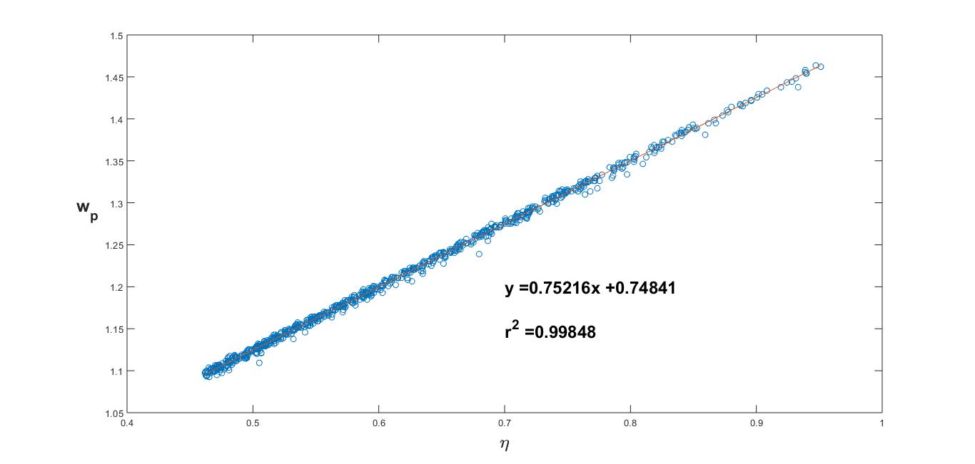
Figure 1. Random Coordinates

We graph $w_{p}(\mathbf{a})$ against $\eta(\mathbf{a})$ for $\mathbf{a}$ chosen randomly on a logarithmic scale and eight $130$-digit values of $q$, as described in Section 3. Figure 1 suggests the following linear relation between $w_{p}(\mathbf{a})$ and $\eta(\mathbf{a})$

(1.4) $$w_{p}(\mathbf{a})=\frac{3}{4}(1+\eta(\mathbf{a}))+o_{q}(1).$$

We give further numerical evidences that supports the above relation in Section 3. Moreover, we prove the following theorem in Section 2.

Theorem 1.5.

Assume $d\geq 3,$ Conjecture 1.1, and $p\leq\log(q)$. We have

$$w_{p}(\mathbf{a})\leq\frac{d-1}{d}(1+\eta(\mathbf{a}))+O(\log\log(q)/\log(q)),$$

where the implicit constant in $O(\log\log(q)/\log(q))$ only depends on $\gamma$ and $C_{\gamma}$ defined in Conjecture 1.1 and it is independent of $p$, $q,$ and $\mathbf{a}.$

Based on our numerical results and Theorem 1.5, we conjecture the following optimal upper bound on $w_{p}(\mathbf{a})$ for every $\mathbf{a}\in S^{d-2}(\mathbb{Z}/q\mathbb{Z})\subset S^{d}(\mathbb{Z}/q\mathbb{Z}).$

Conjecture 1.6.

Let $\mathbf{a}\in S^{d-2}(\mathbb{Z}/q\mathbb{Z})\subset S^{d}(\mathbb{Z}/q\mathbb{Z})$, $p\leq\log(q)$ be a prime number and $d\geq 3$. We have

(1.5) $$w_{p}(\mathbf{a})\leq\frac{d-1}{d}(1+\eta(\mathbf{a}))+O(\log\log(q)/\log(q)),$$

where the implicit constant in $O(\log\log(q)/\log(q))$ only depends on $d$ and it is independent of $p$, $q,$ and $\mathbf{a}.$

Remark 1.7.

By Theorem 1.2 and Theorem 1.4, $w_{p}(\mathbf{a})$ and $\eta(\mathbf{a})$ are computable in polynomial-time in $\log(q).$ Our algorithm for $d=4$ [HMS⁺18] has been implemented and it runs and terminates quickly for $q\sim 10^{100}.$ We verify Conjecture 1.6 for various values of $q$ and $\mathbf{a}$ in Section 3.

We expect that the upper bound (1.5) to be sharp for a generic $\mathbf{a}\in S^{d-2}(\mathbb{Z}/q\mathbb{Z})\subset S^{d}(\mathbb{Z}/q\mathbb{Z})$ and prime $p\leq\log(q).$ More precisely, we expect that

(1.6) $$w_{p}(\mathbf{a})=\frac{d-1}{d}(1+\eta(\mathbf{a}))+O(\log\log(q)/\log(q))$$

for fixed $\mathbf{a}\in S^{d-2}(\mathbb{\mathbb{missing}}{Z}/q\mathbb{Z})\subset S^{d}(\mathbb{\mathbb{missing}}{Z}/q\mathbb{Z}),$ and all but tiny fractions of primes $1\leq p\leq\log(q).$ Moreover, by the equidistribution of covolume-1 lattices $\frac{1}{q^{1/(d-1)}}\mathcal{L}(\mathbf{a})$ in the space of the unimodular lattices, for all but a tiny fractions of $\mathbf{a}\in S^{2}(\mathbb{\mathbb{missing}}{Z}/q\mathbb{Z})\subset S^{4}(\mathbb{\mathbb{missing}}{Z}/q\mathbb{Z}),$ we have $\eta(\mathbf{a})=1/(d-1)+O(\log\log(q)/\log(q)).$ It is also conjectured for $d\geq 3$ that $w_{p}(\mathbf{a})=1+O(\log\log(q)/\log(q))$ for all but a tiny fractions of $\mathbf{a}\in S^{d-2}(\mathbb{\mathbb{missing}}{Z}/q\mathbb{Z})\subset S^{d}(\mathbb{\mathbb{missing}}{Z}/q\mathbb{Z}).$ Hence, the identity (1.6) holds for a generic choice of parameters. Note that $\frac{1}{d-1}\leq\eta(a)\leq 1.$ Hence, we expect that the diophantine exponent $w_{p}(\mathbf{a})$ to be dense in the interval $[1,2-2/d]$ as $q\to\infty$. We give strong numerical evidence for this in Section 3.

1.3. Outline of the proofs

We give an outline of the proof of Theorem 1.2. The proof is based on induction on $d.$ The base case $d=3$ was essentially proved in the previous work of the third author [Sar17a, Theorem 1.10]. Our algorithm starts with searching for the lattice points of $\mathcal{L}(\mathbf{a})$ inside a convex region defined by the intersection of two balls. There is a similar step in the work of Ross and Selinger [RS16]. Sarnak and Ori [PS18] explained this step in terms of Lenstra’s work [Len83]. If the convex region is defined by a system of linear inequalities in a fixed dimension then the general result of Lenstra [Len83] implies this search is polynomially solvable. We use a variant of Lenstra’s argument that is developed in [Sar17a, Theorem 1.10] and Conjecure 1.1 to reduce the problem to dimension $d-1$. At the final stage of our algorithm, we need to represent a given integers $m$ as a sum of two squares if it is possible. We apply Pollard’s rho algorithm to factor $m$ into primes, and check if all the prime factors with the odd exponent are congruent to $1$ mod 4. Finally, we use Schoof’s algorithm [Sch85] to express each prime divisor $p\equiv 1~{}\mathrm{mod}~{}4$ as a sum of two squares. An important feature of our algorithm is that it has been implemented for $d=4$ [HMS⁺18] and $d=3$ [Sar17b], and it runs and terminates quickly.

Acknowledgements

We thank Brandon Boggess for his help for implementing the code of Theorem 1.2. We also thank Professor Peter Selinger for publicly providing a very useful Haskell package (newsynth) which was used in our code.

2. Proof of Theorem 1.2 and 1.4

2.1. $\delta$-LLL reduced basis

In this section we define a $\delta$-LLL reduced basis of $\mathbb{R}^{d},$ and give a proof of Theorem 1.4. We cite a theorem due to Babai on the shape of the LLL-reduced basis. We refer the reader to [LLL82, Section 1] for a detailed discussion of the LLL-algorithm. We first recall the Gram-Schmidt process.

Definition 2.1.

Let $\mathbf{v}_{1},\dots,\mathbf{v}_{k}$ be $k$ linearly independent vectors in $\mathbb{R}^{n}.$ The Gram-Schmidt orthogonalization of $\mathbf{v}_{1},\dots,\mathbf{v}_{k}$ is defined inductively by $\tilde{\mathbf{v}}_{i}=\mathbf{v}_{i}-\sum_{j=1}^{i-1}\mu_{i,j}\tilde{\mathbf{v}}_{j},$ where $\mu_{i,j}:=\frac{\langle\mathbf{v}_{i},\tilde{\mathbf{v}}_{j}\rangle}{\langle\tilde{\mathbf{v}}_{j},\tilde{\mathbf{v}}_{j}\rangle}.$

Next, we define a $\delta$-LLL reduced basis of $\mathbb{R}^{d}$ for any $1/4<\delta<1.$

Definition 2.2.

A basis $\{\mathbf{v}_{1},\dots,\mathbf{v}_{d}\}\subset\mathbb{R}^{d}$ is a $\delta$-LLL reduced basis if the following holds:

1. $|\mu_{i,j}|\leq 1/2$, for every $1\leq i\leq n$, and $j<i,$

2. $\delta|\tilde{\mathbf{v}}_{i}|^{2}\leq|\mu_{i+1,i}\tilde{\mathbf{v}}_{i}+\tilde{\mathbf{v}}_{i+1}|^{2}$ for for every $1\leq i<n.$

Remark 2.3.

By [LLL82, Proposition 1.26], the LLL-algorithm transforms a given basis $B$ of a lattice $\mathcal{L}\subset\mathbb{Z}^{d}$ in $O(d^{4}\log(M(B)))$ operatins into a $\delta$-LLL reduced basis of $\mathbb{R}^{d}$, where $M(B)$ is defined in (1.3).

We cite the following theorem from [Bab86, Theorem 5.1].

Theorem 2.4 (Babai).

Let $\{\mathbf{v}_{1},\dots,\mathbf{v}_{d}\}$ be a $\delta-$LLL reduced basis with $\delta=3/4.$ Let $\theta_{k}$ denote the angle between $\mathbf{v}_{k}$ and the linear subspace $U_{k}=\sum_{j\neq k}\mathbb{R}\mathbf{v}_{j}.$ Then, for every $1\leq k\leq d,$

$$\sin\theta_{k}\geq(\frac{\sqrt{2}}{3})^{d}.$$

We give a proof of Theorem 1.4.

Proof.

We give an LLL-reduced basis for the lattice $\mathcal{L}(\mathbf{a}).$ Assume the $a_{0}\not\equiv 0~{}\mathrm{mod}~{}q.$ Let $|\tilde{a}_{0}|\leq\frac{q-1}{2}$ be the integer such that $\tilde{a}_{0}\equiv(a_{0})^{-1}~{}\mathrm{mod}~{}q$. Let $v_{0}:=(q,0,\dots,0)\in L(\mathbf{a}),$ and

$$v_{i}:=(-\tilde{a}_{0}a_{i},\delta_{1,i},\dots,\delta_{d-2,i})$$

for $1\leq i\leq d-2,$ where $\delta_{i,j}=1$ if $i=j,$ and $\delta_{i,j}=0$ otherwise. Since the co-volume of $\mathcal{L}(\mathbf{a})$ is $q$, it follows that $\{v_{0},\dots,v_{d-2}\}$ is a $\mathbb{Z}$ basis for $\mathcal{L}(\mathbf{a}).$ We apply the LLL basis reduction algorithm on $\{v_{0},\dots,v_{d-2}\}$ for $\delta=3/4$ and obtain a 3/4-LLL reduced basis $B_{L}:=\{\mathbf{u}_{0},\dots,\mathbf{u}_{d-2}\}$ for $\mathcal{L}(\mathbf{a})$ in $O(\log(q))$ steps; see Remark 2.3. By [LLL82, Proposition 1.12], we have

$$\min_{B}M(B)\leq M(B_{L})\leq 2^{(d-2)/2}\min_{B}M(B).$$

Hence,

$$0\leq\log_{q}(M(B_{L}))-\eta(\mathbf{a})\leq\frac{d-2}{2\log_{2}q}=O_{d}(1/\log q).$$

This concludes the proof of Theorem 1.4. ∎

2.2. Proof of Theorem 1.2

Recall the notations while formulating Theorem 1.2. Let $\mathbf{a}=(a_{0},\dots,a_{d}),$ where $a_{d-1}\equiv a_{d}\equiv 0~{}\mathrm{mod}~{}q$. Assume that $\mathbf{s}:=(\frac{n_{0}}{p^{h}},\dots,\frac{n_{d}}{p^{h}})\in S^{d}(\mathbb{Z}[1/p])$ is a minimal lift of $\mathbf{a},$ where $n_{i}\in\mathbb{Z}.$ Hence, we have

$$\begin{split}&n_{0}^{2}+\dots+n_{d}^{2}=p^{2h},\\ &n_{i}\equiv p^{h}a_{i}~{}\mathrm{mod}~{}q\text{ for }0\leq i\leq d.\end{split}$$

More generally, let $N\leq q^{A}$ for some fixed $A>0$ be an integer, and $b_{i}\in\mathbb{Z}$ for $0\leq i\leq d-2,$ where $\sum_{i=0}^{d-2}b_{i}^{2}\equiv N~{}\mathrm{mod}~{}q$. Theorem 1.2 follows from the following Proposition.

Proposition 2.5.

Assume $(*)$ and $d\geq 3$, we develop a polynomial-time algorithm in $\log(q)$ that finds a solution $(t_{0},\dots,t_{d})\in\mathbb{Z}^{d+1}$, if it exists, to

(2.1) $$(qt_{0}+b_{0})^{2}+\dots+(qt_{d-2}+b_{d-2})^{2}+(qt_{d-1})^{2}+(qt_{d})^{2}=N.$$

If there is no integral solution, it terminates in polynomial-time in $\log(q).$

Proof of Theorem 1.2.

For $0\leq h\leq 4\log_{p}q,$ let $N=p^{2h}$ and $b_{i}\equiv a_{i}p^{h}~{}\mathrm{mod}~{}q$ for $0\leq i\leq d-2.$ By theorem [Sar15a, Theorem 1.2] the diophantine equation (2.1) has a solution for every $(3+o_{q}(1))\log_{p}q\leq h\leq 4\log_{p}q.$ Our goal is to find the smallest $h$ such that the equation (2.1) has a solution, and then find a solution to the equation (2.1). For $0\leq h\leq 4\log_{p}q,$ apply the algorithm in Proposition 2.5, in order to find an integral solution to the equation 2.1. If there exits such a solution $(t_{h,0},\dots,t_{h,d}),$ then

$$\mathbf{s}_{h}:=(\frac{qt_{h,0}+b_{0}}{p^{h}},\dots,\frac{qt_{h,d-2}+b_{d-2}}{p^{h}},\frac{qt_{h,d-1}}{p^{h}},\frac{qt_{h,d}}{p^{h}})$$

is a lift for $\mathbf{a}\in S^{d}(\mathbb{Z}[1/p]).$ Otherwise the algorithm in Proposition 2.5 terminates in polynomial-time in $\log(q)$ with no solutions, and $\mathbf{a}$ does not have any integral lift $\mathbf{s}\in S^{d}(\mathbb{Z}[1/p])$ with $H(\mathbf{s})=p^{h}$. We have a lift $\mathbf{s}_{h}$ for every $(3+o_{q}(1))\log_{p}q\leq h\leq 4\log_{p}q,$ let $h_{min}$ be the smallest exponent $0\leq h\leq 4\log_{p}q$ such that the lift $\mathbf{s}_{h}$ exists. Then $\mathbf{s}_{h_{min}}$ is a minimal lift and this concludes the proof of Theorem 1.2. ∎

Next, we prove two auxiliary lemmas and finally give a proof of Proposition 2.5. By rearranging (2.1), we have

(2.2) $$t_{d-1}^{2}+t_{d}^{2}=N/q^{2}-(t_{0}+b_{0}/q)^{2}-\dots-(t_{d-2}+b_{d-2}/q)^{2}.$$

Let $Q(\mathbf{t}):=N/q^{2}-|\mathbf{t}+\frac{1}{q}\mathbf{b}|^{2},$ where $\mathbf{t}=(t_{0},\dots,t_{d-2}),$ $\mathbf{b}=(b_{0},\dots,b_{d-2})$ and $|.|$ is the Euclidean norm.

Recall the definition of $A_{Q,r}$ from (1.1), where $r>0$ is some real number. By Conjecture 1.1, if $|A_{Q,r}|>C_{\gamma}(\log N)^{\gamma}$ then the equation (2.2) has a solution, where $\mathbf{t}\in A_{Q,r}.$ Let $k:=(N-|\mathbf{b}|^{2})/q$. Since $|\mathbf{b}|^{2}\equiv N~{}\mathrm{mod}~{}q$, $k\in\mathbb{Z}.$ We can further rearrange (2.2):

$$t_{d-1}^{2}+t_{d}^{2}=(k-2\langle\mathbf{b},\mathbf{t}\rangle)/q-|\mathbf{t}|^{2}.$$

Note that $\mathbf{t}\in A_{Q,r}$ iff the following two conditions are satisfied:

• Condition 1: $|\mathbf{t}+\frac{1}{q}\mathbf{b}|^{2}\leq N/q^{2}$, and $|\mathbf{t}|<r.$

• Condition 2: $2\langle\mathbf{b},\mathbf{t}\rangle\equiv k~{}\mathrm{mod}~{}q$.

We first focus on Condition 2. Without loss of generality, we assume that $a_{0}\not\equiv 0$ mod $q$. Then $2b_{0}\equiv 2p^{h}a_{0}\not\equiv 0~{}\mathrm{mod}~{}q$ and $2b_{0}$ has an inverse mod $q$. Let $\tilde{b}_{0}\leq\frac{q-1}{2}$ be the integer such that $\tilde{b}_{0}\equiv(2b_{0})^{-1}~{}\mathrm{mod}~{}q$. Then $\mathbf{t}_{0}:=(k\tilde{b}_{0},0,\dots,0)$ is a solution for the congruence equation in Condition (2). Since $p^{h}\mathbf{a}\equiv\mathbf{b}~{}\mathrm{mod}~{}q$, the integral solutions of Condition (2) are the translation of the lattice points of $\mathcal{L}(\mathbf{a})$ by $\mathbf{t}_{0}.$ Let $\{\mathbf{u}_{0},\dots,\mathbf{u}_{d-2}\}$ be the 3/4-LLL reduced basis for $\mathcal{L}(\mathbf{a})$ that is defined in the proof of Theorem 1.4. We write

$$\mathbf{t}_{0}+\frac{1}{q}\mathbf{b}=\sum_{i=0}^{d-2}c_{i}\mathbf{u}_{i},$$

for sum $c_{i}\in\frac{1}{q^{2}}\mathbb{Z}.$ Let $\tilde{\mathbf{t}}_{0}=\sum_{i=0}^{d-2}r_{i}\mathbf{u}_{i},$ where $|r_{i}|\leq 1/2$ and $c_{i}-r_{i}\in\mathbb{Z}$ for every $0\leq i\leq d-2.$ Assume that $\mathbf{t}\in\mathbb{Z}^{d-1}$ satisfies Condition (2). Then, there exists a one to one correspondence between $\mathbf{t}$ and $\mathbf{x}:=(x_{0},\dots,x_{d-2})\in\mathbb{Z}^{d-1}$, such that:

$$\tilde{\mathbf{t}}_{0}+\sum_{i=0}^{d-2}x_{i}\mathbf{u}_{i}=\mathbf{t}+\frac{1}{q}\mathbf{b}.$$

Let

$$F(\mathbf{x}):=N/q^{2}-|\tilde{\mathbf{t}}_{0}+\sum_{i=0}^{d-2}x_{i}\mathbf{u}_{i}|^{2}.$$

Note that $F(\mathbf{x})=Q(\mathbf{t})$ by the above correspondence, and $F(\mathbf{x})\in\mathbb{Z}$ for every $\mathbf{x}\in\mathbb{Z}^{d-1}.$ Clearly Condition (1) is satisfied if and only if $F\geq 0$.

We prove two general lemmas for listing the positive values of $F(\mathbf{x})$. Assume that $\{\mathbf{w}_{1},\dots,\mathbf{w}_{m}\}$ is a $3/4$-LLL basis for $\mathbb{R}^{m}.$ Let $\tilde{\mathbf{w}}_{0}=\sum_{i=1}^{m}s_{i}\mathbf{w}_{i},$ where $|s_{i}|<1/2.$ Define

$$H(x_{1},\dots,x_{m}):=M^{2}-|\tilde{\mathbf{w}}_{0}+\sum_{i=1}^{m}x_{i}\mathbf{w}_{i}|^{2},$$

where $M$ is some real number.

Lemma 2.6.

Assume that $\alpha|\mathbf{w}_{k}|>M$ for some $\alpha>0$, and $H(x_{1},\dots,x_{m})>0$, then

$$|x_{k}|\leq\alpha(\frac{3}{\sqrt{2}})^{m}+1.$$

Proof.

Since $H(x_{1},\dots,x_{m})>0,$ we have

$$0<H(x_{1},\dots,x_{m})\leq M^{2}-\big{(}\sin\theta_{k}(x_{k}+s_{k})|\mathbf{w}_{k}|\big{)}^{2}.$$

By Theroem 2.4 and $\alpha|\mathbf{w}_{k}|>M,$ we have

$$\big{|}\sin\theta_{k}(x_{k}+s_{k})|\mathbf{w}_{k}|\big{|}\geq(\frac{\sqrt{2}}{3})^{m}(|x_{k}|-1/2)\frac{M}{\alpha}.$$

Hence,

$$|x_{k}|\leq\alpha(\frac{3}{\sqrt{2}})^{m}+1/2.$$

This concludes the lemma. ∎

Lemma 2.7.

Assume that $2m|\mathbf{w}_{i}|<M$ for $1\leq i\leq m$. Let $A_{i}:=\frac{M}{m|\mathbf{w}_{i}|}-1/2$ and $C:=\prod_{i=1}^{m}[-A_{i},A_{i}].$ Then $H(\mathbf{x})$ is positive for every $\mathbf{x}\in C$ and negative outside $2m(\frac{3}{\sqrt{2}})^{m}C$.

Proof.

Recall that $H(x_{1},\dots,x_{m})=M^{2}-|\tilde{\mathbf{w}}_{0}+\sum_{i=1}^{m}x_{i}\mathbf{w}_{i}|^{2},$ and $\tilde{\mathbf{w}}_{0}=\sum_{i=1}^{m}s_{i}\mathbf{w}_{i},$ where $|s_{i}|<1/2.$ Assume that $\mathbf{x}\in C.$ By the triangle inequality

$$H(\mathbf{x})\geq M^{2}-\big{(}\sum_{i=1}^{m}(|x_{i}|+1/2)|\mathbf{w}_{i}|\big{)}^{2} \geq M^{2}-\big{(}\sum_{i=1}^{m}(A_{i}+1/2)|\mathbf{w}_{i}|\big{)}^{2}$$

$$\geq M^{2}-M^{2}=0.$$

Next, we show that $H$ is negative outside $2m(\frac{3}{\sqrt{2}})^{m}C.$ Assume that $\mathbf{y}:=(y_{1},\dots,y_{m})\not\in 2m(\frac{3}{\sqrt{2}})^{m}C.$ Hence, there exits $1\leq k\leq m$ such that $|y_{k}|\geq 2m(\frac{3}{\sqrt{2}})^{m}A_{k}.$ By Theorem 2.4 and the assumption $2m|\mathbf{w}_{k}|<M$, we obtain

$$F(\mathbf{y}) \leq M^{2}-\big{(}\sin\theta_{k}(y_{k}+r_{k})|\mathbf{w}_{k}|\big{)}^{2}$$

$$\leq M^{2}-\Big{(}(\frac{\sqrt{2}}{3})^{m}\big{(}2m(\frac{3}{\sqrt{2}})^{m}(\frac{M}{m|\mathbf{w}_{k}|}-1/2)-1/2\big{)}|\mathbf{w}_{k}|\Big{)}^{2}<0$$

This concludes our lemma. ∎

Finally, we give a proof of Proposition 2.5.

Proof of Proposition 2.5.

Recall the notations and the assumptions while formulating Proposition 2.5. We develop an algorithm that finds a solution to the equation (2.2) in polynomial-time in $\log(q),$ and if it does not have a solution, it terminates in polynomial-time in $\log(q)$.

First, assume that $2(d-1)|\mathbf{u}_{i}|<\frac{N}{\sqrt{q}}$ for every $1\leq i\leq d-1.$ By Lemma 2.7, there exists a box $C$ such that $F(\mathbf{x})$ is positive inside $C$ and it is negative outside $2(d-1)(\frac{3}{\sqrt{2}})^{d-1}C$. We consider two cases.

• Case 1: if $|C|\leq C_{\gamma}\log(N)^{\gamma},$

• Case 2: if $|C|>C_{\gamma}\log(N)^{\gamma}.$

where $|C|=\prod_{i=0}^{d-2}A_{i},$ $C_{\gamma}$ and $\gamma$ are defined in Conjecture 1.1.

For Case 1, we check if any point $\mathbf{x}\in 2(d-1)(\frac{3}{\sqrt{2}})^{d-1}C$ gives a solution to the equation 2.2 as follows. We factor $F(\mathbf{x})$ in polynomial-time in $\log(q)$ into its prime powers, by our assumed polynomial-time factoring algorithm. We check if all the prime factors with the odd exponent are congruent to $1$ mod 4. Finally, we use Schoof’s algorithm [Sch85] to express each prime divisor $p\equiv 1~{}\mathrm{mod}~{}4$ as a sum of two squares. Since $|C|\leq C_{\gamma}\log(N)^{\gamma},$ this conduces the proof of Proposition 2.5.

For Case 2, by Conjecture 1.1, there exists $\mathbf{x}\in C$ such that $F(\mathbf{x})=t_{d-1}^{2}+t_{d}^{2}$ for some $t_{d-1},t_{d}\in\mathbb{Z},$ where $|\mathbf{x}|\leq C_{\gamma}\log(N)^{\gamma}.$ Similarly, we find such $|\mathbf{x}|\leq C_{\gamma}\log(N)^{\gamma}$ in polynomial time. This conduces the proof of Proposition 2.5 if $2(d-1)|\mathbf{u}_{i}|<\frac{N}{\sqrt{q}}$ for every $1\leq i\leq d-1.$

Otherwise, there exists $0\leq k\leq d-2$ such that $2(d-1)|\mathbf{u}_{k}|>\frac{N}{\sqrt{q}}.$ By Lemma 2.6,

$$|x_{k}|\leq 2(d-1)(\frac{3}{\sqrt{2}})^{d-1}+1.$$

Since $d$ is fixed, there are only a bounded number of choices for $x_{k}\in\mathbb{Z}.$ Let $x_{k}=l$ for some $l\in\mathbb{Z},$ where $|l|\leq 2(d-1)(\frac{3}{\sqrt{2}})^{d-1}+1.$ Hence,

$$F(\mathbf{x}):=N/q^{2}-|\tilde{\mathbf{t}}_{0}+l\mathbf{u}_{k}+\sum_{i\neq k}^{d-2}x_{i}\mathbf{u}_{i}|^{2}.$$

We write uniquely $\tilde{\mathbf{t}}_{0}+l\mathbf{u}_{k}=\mathbf{u}_{k,1}+\mathbf{u}_{k,2},$ where $\mathbf{u}_{k,1}=\sum_{i\neq k}\alpha_{i}\mathbf{u}_{i}$ and $\mathbf{u}_{k,2}$ is orthogonal to $\sum_{i\neq k}\mathbb{R}\mathbf{u}_{i}.$ Hence,

$$F(\mathbf{x})=M-|\tilde{\mathbf{w}}_{0}+\sum_{i\neq k}^{d-2}y_{i}\mathbf{u}_{i}|^{2}$$

where $M:=(N/q^{2}-|\mathbf{u}_{k,2}|^{2}),$ $\tilde{\mathbf{w}}_{0}:=\sum_{i\neq k}s_{i}\mathbf{u}_{i},$ where $|s_{i}|\leq 1/2$ and $s_{i}-\alpha_{i}\in\mathbb{Z},$ and $y_{i}=x_{i}+\alpha_{i}-s_{i}.$ Let

$$G_{l,k}(\mathbf{y}):=M-|\tilde{\mathbf{w}}_{0}+\sum_{i\neq k}^{d-2}y_{i}\mathbf{u}_{i}|^{2}.$$

Next, we use a similar argument as in the beginning of our proof. We assume that $2(d-1)|\mathbf{u}_{i}|<M$ for all $i\neq k,$ and proceed with the same argument on $G_{l,k}(\mathbf{y})$ as $F(\mathbf{x})$. We either find a solution for the equation (2.2), or find another variable with bounded value. Since the dimension $d$ is bounded this algorithm terminates in polynomial time in $\log(q).$ This completes the proof of Proposition 2.5. ∎

Finally, we give a proof of Theorem 1.5

Proof.

Assume that

$$h\geq(\log_{p}q)\Big{(}1+\eta(\mathbf{a})+\frac{2d+\log_{2}2C_{\gamma}+\gamma\log_{2}5\log q}{\log_{2}(q)}\Big{)}.$$

Let $B_{L}:=\{\mathbf{u}_{0},\dots,\mathbf{u}_{d-2}\}$ be the LLL-reduced basis that is introduced in the proof of Theorem 1.4. It follows from the proof of Theorem 1.4 that

$$\eta(\mathbf{a})+\frac{d}{\log_{2}(q)}\geq\log_{q}(M(B_{L})).$$

Hence, for every $0\leq i\leq d-2$, we have

$$h\geq(\log_{p}q)\Big{(}1+\log_{q}(|\mathbf{u}_{i}|)+\frac{d+\log_{2}2C_{\gamma}+\gamma\log_{2}5\log q}{\log_{2}(q)}\Big{)}.$$

Let $N:=p^{2h}$, we have

$$\frac{\sqrt{N}}{q}\geq 2d|\mathbf{u}_{i}|C_{\gamma}(\log q^{5})^{\gamma}.$$

Assume that $N\leq q^{5},$ then

$$\frac{\sqrt{N}}{q}\geq 2d|\mathbf{u}_{i}|C_{\gamma}(\log N)^{\gamma}.$$

By the proof of Proposition 2.5, if follows that there exists an integral lift $\mathbf{s}\in S^{d}(\mathbb{Z}[1/p])$ with $H(\mathbf{s})=p^{h}.$ Therefore,

$$w_{p}(\mathbf{a})\leq\frac{d-1}{d}(1+\eta(\mathbf{a}))+O_{d}(\log\log(q)/\log(q)).$$

This concludes the proof of Theorem 1.5. ∎

3. Numerical results

We now give numerical evidence for Conjecture 1.1 by testing identity 1.4 for $d=4$. Figure 1, shown in the introduction, was produced by choosing the three non-zero coordinates in $S^{4}(\mathbb{Z}/q\mathbb{Z})$ randomly on a logarithmic scale. This was done specifically by first choosing an integer $r$ randomly from $60$ to $125$ for each coordinate, then choosing an integral representative of the coordinate randomly from $0$ to $10^{-r}q$. This was done $100$ times for each of eight $130$-digit primes listed below, and all points were included in the figure:

• $q_{1}=$ 8 7 1 4 7 7 2 9 7 6 3 8 1 6 9 7 8 5 9 5 5 7 9 6 5 3 5 5 7 9 1 7 4 5 9 9 7 9 8 7 7 2 8 3 0 0 2 2 6 8 1 2 7 3 2 5 1 9 7 0 2 2 5 0 4 6 3 3 2 9 2 6 5 8 2 6 0 3 3 2 6 8 9 2 6 1 7 1 6 1 0 3 9 2 2 1 1 7 5 0 0 4 4 9 5 7 7 1 9 8 9 6 3 2 0 7 7 6 7 9 4 5 5 5 1 4 6 5 8 1

• $q_{2}=$ 4 4 8 6 8 4 7 1 8 8 0 5 2 9 1 9 9 9 8 8 4 0 4 4 5 6 3 3 1 9 7 1 8 5 8 3 7 4 1 2 6 9 4 5 5 5 9 2 0 4 7 0 5 0 5 2 7 2 9 6 0 8 8 0 2 9 2 1 1 8 6 9 9 5 7 4 8 6 0 4 1 9 6 0 2 0 2 5 0 7 5 6 3 9 1 9 7 6 3 9 9 7 3 6 2 3 2 4 1 1 7 4 5 5 4 6 4 0 2 3 9 9 4 0 4 6 8 4 9 1

• $q_{3}=$ 3 0 0 7 4 8 1 5 1 9 7 7 4 8 4 1 7 0 0 4 4 7 1 6 9 1 0 3 6 9 9 4 8 0 4 7 9 2 5 7 0 7 5 1 5 8 0 0 4 4 2 9 1 7 2 5 0 5 4 9 3 1 6 9 6 2 4 2 1 1 7 3 8 1 6 5 6 2 6 2 0 4 2 2 1 6 5 3 1 1 5 5 1 8 1 7 1 8 9 5 1 2 4 2 5 4 9 5 5 0 50 1 9 2 4 7 6 6 4 7 3 9 3 2 4 0 5 4 9

• $q_{4}=$ 1 1 8 2 9 1 1 1 4 1 4 9 7 5 4 1 1 4 0 5 8 6 6 1 5 3 5 9 2 3 0 2 4 3 5 9 2 8 3 4 25 9 9 3 5 9 5 1 4 5 7 9 2 3 8 9 0 1 0 0 9 0 1 1 4 3 7 2 4 7 0 2 2 9 5 7 5 0 5 4 3 1 8 0 7 5 7 8 8 6 0 0 3 7 6 2 2 5 0 8 2 2 0 1 4 7 7 0 4 3 2 4 0 6 7 8 5 9 7 5 2 2 0 7 1 2 5 5 1

• $q_{5}=$ 5 4 5 2 2 1 2 1 5 1 8 4 4 2 6 4 4 5 3 1 1 5 5 2 1 7 7 0 3 6 2 7 1 2 8 1 5 3 0 0 4 5 6 7 8 8 0 7 3 8 7 0 2 6 0 6 3 7 1 7 2 0 0 6 4 1 4 9 8 7 4 7 9 9 1 4 1 5 0 8 3 1 8 2 1 2 0 2 2 5 9 8 6 2 0 9 1 3 7 3 7 4 1 7 3 8 5 1 1 5 7 9 6 2 9 0 4 0 7 3 2 9 0 9 1 9 4 8 8 3

• $q_{6}=$ 6 5 3 9 0 1 0 9 3 5 8 3 6 2 4 8 6 9 8 1 3 0 7 9 7 8 9 5 0 0 9 7 0 2 3 6 5 5 0 2 8 9 4 5 0 6 1 0 9 6 0 0 3 3 5 0 0 3 5 4 9 6 4 6 8 0 7 8 4 8 5 9 7 7 7 0 3 8 7 6 0 7 6 1 2 7 6 7 2 8 5 5 5 8 4 4 0 8 8 9 4 4 4 1 3 2 8 2 4 6 9 6 9 1 4 1 1 3 6 0 3 5 6 9 7 1 3 1 5 2

• $q_{7}=$ 1 9 6 6 6 0 5 1 7 0 3 5 1 8 8 3 0 0 3 6 6 9 3 8 1 3 2 6 7 2 6 2 5 4 8 6 5 0 9 5 1 8 5 7 3 6 1 5 9 6 1 0 5 1 1 2 9 0 3 1 7 2 3 8 3 1 5 2 3 2 4 2 1 3 3 5 3 4 0 7 8 7 9 5 3 2 2 3 3 7 4 9 5 0 9 7 1 8 5 0 2 8 7 5 1 7 5 6 1 7 2 5 1 8 3 5 2 5 3 4 9 9 0 1 7 2 9 7 9 2

• $q_{8}=$ 4 5 7 8 4 8 7 2 7 4 2 0 8 4 8 2 7 2 2 0 6 7 2 3 8 0 3 9 3 4 0 3 6 9 5 8 1 5 9 7 5 4 2 8 5 9 6 1 0 6 2 8 5 6 8 5 2 5 9 8 4 9 4 4 9 5 3 6 4 9 1 7 8 9 3 7 3 5 1 2 6 5 6 3 8 9 9 8 8 5 6 7 6 4 6 3 9 7 8 5 6 8 6 8 2 9 3 8 0 2 0 2 6 3 7 9 1 3 3 2 9 7 3 9 2 3 5 3 2 8

3.1. Generic Coordinates

There are several cases which are worthy of special consideration. The generic element of $S^{2}(\mathbb{Z}/q\mathbb{Z})$ has coordinates of size $q$, so we expect $\eta(\mathbf{a})=1/3$ and $w_{p}(\mathbf{a})=1$ for most lattices. Figure 2 shows that this is indeed the case, using the same primes and number of points as Figure 1. The coordinates are chosen between $0$ and $q$ on a linear, rather than logarithmic scale. The horizontal lines observed on the small-scale are a result of $H(\mathbf{a})$, and therefore $w_{p}(\mathbf{a})$, taking much more discrete values than $\eta(\mathbf{a})$.

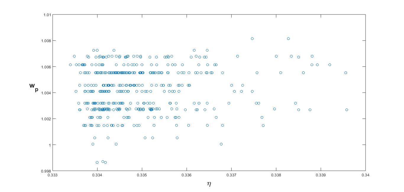
Figure 2. Generic Coordinates

3.2. Small Coordinates

When all coordinates are small, the lattice is quite high in the cusp, and therefore one expects $\eta(\mathbf{a})=1$ and $w_{p}(\mathbf{a})=3/2$, which is observed in Figure 3. Here all coordinates are chosen between $0$ and $10^{-125}q$.

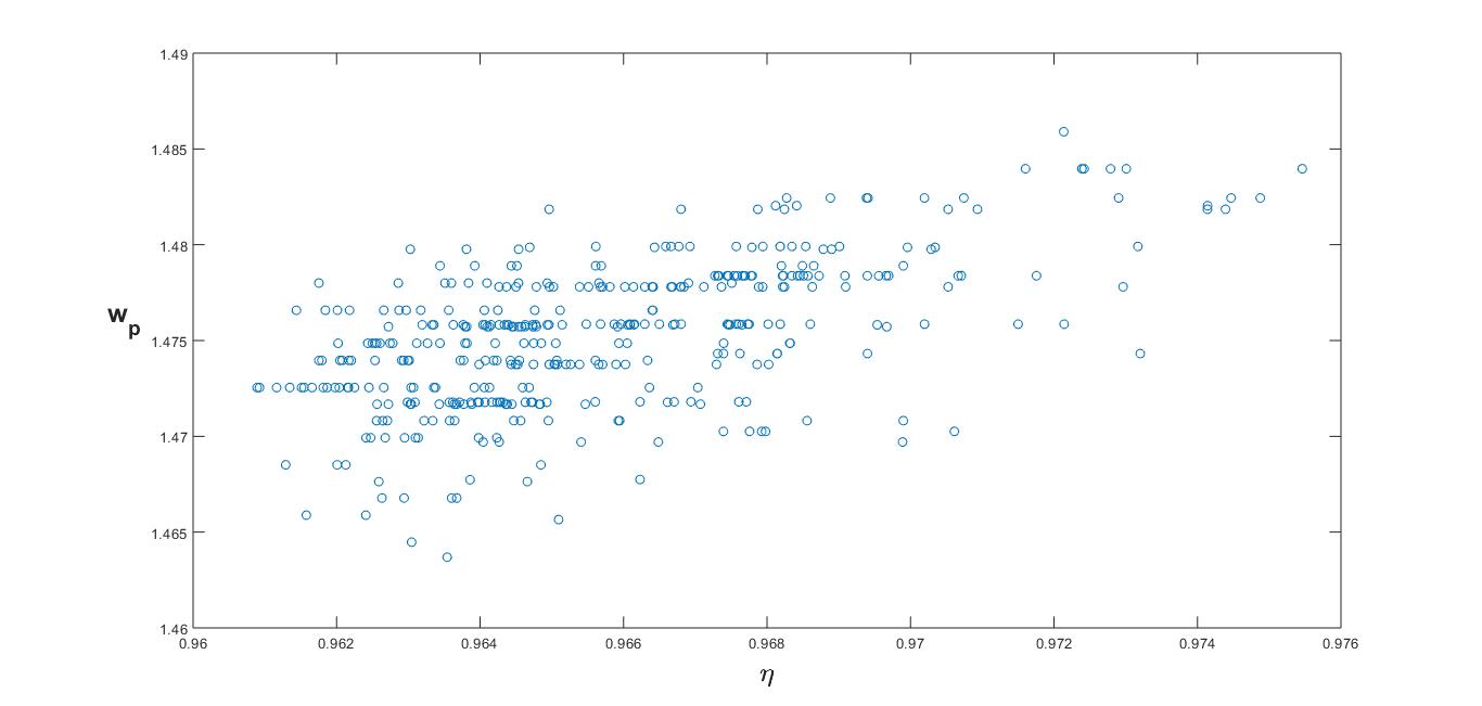
Figure 3. Small Coordinates

3.3. Other Cusp Regions

One can explore additional cusp cases by fixing one or two coordinates and varying the rest on a logarithmic scale. Figures  4 and  5 show that identity 1.4 still holds in these two cases. The fixed coordinate is set to $1$, and the other coordinates are chosen as in Figure 1. Note that in Figure 5, where only one coordinate is large, the lattices are relatively high in the cusp, but the corresponding points still adhere to the theoretical line.

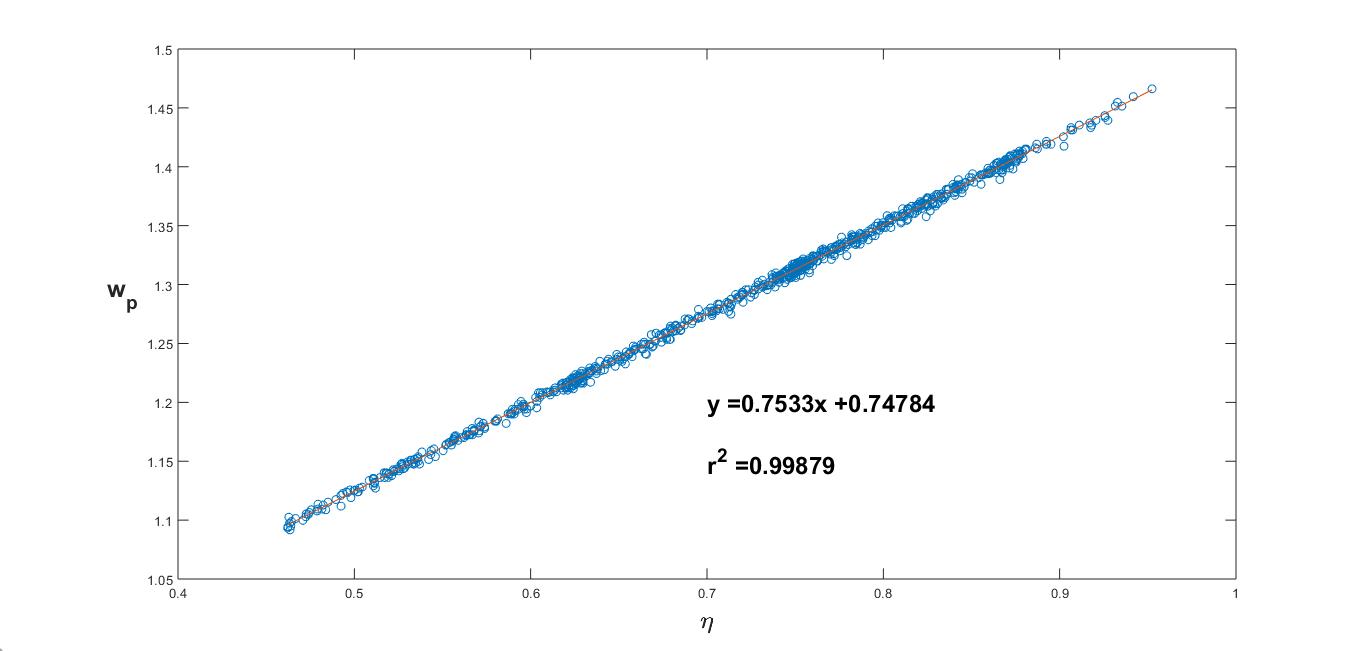
Figure 4. One Coordinate Fixed

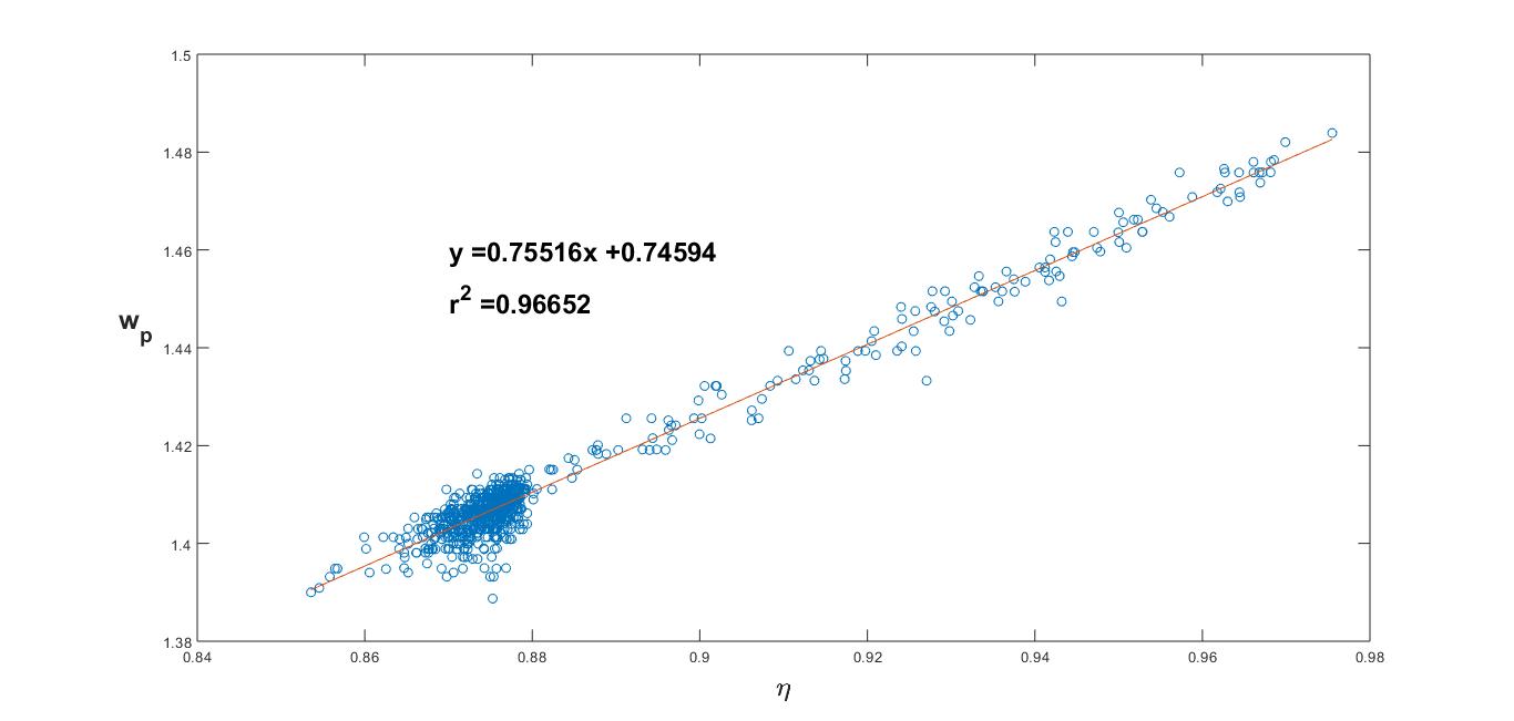
Figure 5. Two Coordinates Fixed

References

- [Bab86] L. Babai. On Lovász’ lattice reduction and the nearest lattice point problem. Combinatorica, 6(1):1–13, 1986.
- [BKS17] T.D. Browning, V. Vinay Kumaraswamy, and R.S. Steiner. Twisted linnik implies optimal covering exponent for . International Mathematics Research Notices, page rnx116, 2017.
- [HMS+18] M. W. Hassan, Y. Mao, N. T. Sardari, R. Smith, and X. Zhu. 5 Squares Algorithm, August 2018. https://gitlab.com/5-Squares-Algorithm/diophantine-approximation.
- [Klo27] H. D. Kloosterman. On the representation of numbers in the form . Acta Math., 49(3-4):407–464, 1927.
- [Len83] H. W. Lenstra, Jr. Integer programming with a fixed number of variables. Math. Oper. Res., 8(4):538–548, 1983.
- [LLL82] A. K. Lenstra, H. W. Lenstra, Jr., and L. Lovász. Factoring polynomials with rational coefficients. Math. Ann., 261(4):515–534, 1982.
- [LPS88] A. Lubotzky, R. Phillips, and P. Sarnak. Ramanujan graphs. Combinatorica, 8(3):261–277, 1988.
- [Mar88] G. A. Margulis. Explicit group-theoretic constructions of combinatorial schemes and their applications in the construction of expanders and concentrators. Problemy Peredachi Informatsii, 24(1):51–60, 1988.
- [PLQ08] Christophe Petit, Kristin Lauter, and Jean-Jacques Quisquater. Full Cryptanalysis of LPS and Morgenstern Hash Functions, pages 263–277. Springer Berlin Heidelberg, Berlin, Heidelberg, 2008.
- [PS18] Ori Parzanchevski and Peter Sarnak. Super-golden-gates for . Adv. Math., 327:869–901, 2018.
- [RS16] Neil J. Ross and Peter Selinger. Optimal ancilla-free approximation of -rotations. Quantum Inf. Comput., 16(11-12):901–953, 2016.
- [Sar15a] N. T Sardari. Optimal strong approximation for quadratic forms. ArXiv e-prints, October 2015.
- [Sar15b] Peter Sarnak. Letter to Scott Aaronson and Andy Pollington on the Solovay-Kitaev Theorem, February 2015. https://publications.ias.edu/sarnak/paper/2637https://publications.ias.edu/sarnak/paper/2637.
- [Sar17a] N. T Sardari. Complexity of strong approximation on the sphere. ArXiv e-prints, March 2017.
- [Sar17b] N. T. Sardari. Navigating LPS Ramanujan Graphs, March 2017. https://gitlab.com/ntalebiz/navigating-lps-ramanujan-graphs.
- [Sar18] Naser T. Sardari. Diameter of ramanujan graphs and random cayley graphs. Combinatorica, Aug 2018.
- [Sch85] René Schoof. Elliptic curves over finite fields and the computation of square roots mod . Math. Comp., 44(170):483–494, 1985.