A Topological Study of Functional Data and Fréchet Functions of Metric Measure Spaces

Abstract

We study the persistent homology of both functional data on compact topological spaces and structural data presented as compact metric measure spaces. One of our goals is to define persistent homology so as to capture primarily properties of the shape of a signal, eliminating otherwise highly persistent homology classes that may exist simply because of the nature of the domain on which the signal is defined. We investigate the stability of these invariants using metrics that downplay regions where signals are weak. The distance between two signals is small if they exhibit high similarity in regions where they are strong, regardless of the nature of their full domains, in particular allowing different homotopy types. Consistency and estimation of persistent homology of metric measure spaces from data are studied within this framework. We also apply the methodology to the construction of multi-scale topological descriptors for data on compact Riemannian manifolds via metric relaxations derived from the heat kernel.

Keywords: persistent homology, functional data, metric-measure spaces.

1 Introduction

This paper investigates ways of producing robust, informative summaries of both functional data on topological spaces and structural data in metric spaces, two problems that permeate the sciences and applications. Many problems involving structural data may be formulated in the realm of metric-measure spaces ($mm$-spaces) $\mathbb{X}_{\alpha}=(X,d_{X},\alpha)$, where $(X,d_{X})$ is a metric space and $\alpha$ is a Borel probability measure on $X$. For example, a dataset $x_{1},\ldots,x_{n}\in X$ may be analyzed via the associated empirical measure $\sum_{i=1}^{n}\delta_{x_{i}}/n$, where $\delta_{x_{i}}$ is the Dirac measure based at $x_{i}$.

The mean of a Euclidean distribution is a most basic statistic that may be generalized to triples $(X,d_{X},\alpha)$ via the Fréchet function $V_{\mathbb{X}_{\alpha}}\colon X\to\mathbb{R}$ defined by

$$V_{\mathbb{X}_{\alpha}}(x)=\int_{X}d^{2}(x,y)\,d\alpha(y)\,.$$ (1)

In the Euclidean case, it is well known that the mean is the unique minimizer of $V_{\mathbb{X}_{\alpha}}$ , provided that $\alpha$ has finite second moment. In the more general setting, a Fréchet mean is a minimizer of $V_{\mathbb{X}_{\alpha}}$, not necessarily unique, thus leading to the concept of Fréchet mean set. One also may consider the local minima of $V_{\mathbb{X}_{\alpha}}$ that often yield valuable additional information about the distribution. The Fréchet mean has received a great deal of attention from many authors (cf. [20, 3, 1]). However, Fréchet mean sets may be difficult to estimate or compare quantitatively, limiting its applicability in data analysis.

Beyond means, a wealth of structural information about $\mathbb{X}_{\alpha}$ typically resides in $V_{\mathbb{X}_{\alpha}}$ (cf. [11, 12]). One of our primary goals is to carry out a topological study of the Fréchet function via persistent homology to uncover and summarize properties of the shape of probability distributions on metric spaces. The study is done in the general setting of Fréchet functions of order $p\geq 1$, defined as

$$V_{p,\mathbb{X}_{\alpha}}(x)=\int_{X}d^{p}(y,x)\,d\alpha(y)\,.$$ (2)

Some authors refer to $V_{p,\mathbb{X}_{\alpha}}$ as the $p$-eccentricity function of $\mathbb{X}_{\alpha}$ (cf. [5]). Closely related to $V_{p,\mathbb{X}_{\alpha}}$ is the function $\sigma_{p,\mathbb{X}_{\alpha}}\colon X\to\mathbb{R}$ defined as

$$\sigma_{p,\mathbb{X}_{\alpha}}(x)=(V_{p,\mathbb{X}_{\alpha}}(x))^{1/p}\,,$$ (3)

which we refer to as the $p$-centrality function of $\mathbb{X}_{\alpha}$. We opt to construct topological summaries for $\mathbb{X}_{\alpha}$ using $\sigma_{p,\mathbb{X}_{\alpha}}$, rather than $V_{p,\mathbb{X}_{\alpha}}$, because barcodes or persistence diagrams derived from $p$-centrality are more amenable to analysis. A key property of Fréchet and centrality functions is that they attenuate the influence of outliers in persistence homology computed from large random samples of a distribution, a fact that is implicit in the stability and consistency results proven in this paper.

We view $\sigma_{p,\mathbb{X}_{\alpha}}\colon X\to\mathbb{R}$ as a “signal” on $X$ and first work in the more general setting of functional data on compact topological spaces. Subsequently, we specialize to centrality functions of $mm$-spaces. In the functional setting, a data object is a triple $\mathbb{X}_{f}:=(X,\tau_{X},f)$, where $(X,\tau_{X})$ is a topological space and $f\colon X\to\mathbb{R}$ is a continuous function. The collection of all such triples is denoted $\mathscr{F}$. We make the convention that large values of $f$ correspond to weak signals. Generally, this is more consistent with the behavior of Fréchet functions that attain larger values in data deserts, far away from concentrations of probability mass (cf. [11]).

In defining persistent homology [16, 25, 15, 5, 14, 8] invariants for $\mathbb{X}_{f}$, there are a few drawbacks in following the standard procedure of using the filtration of $X$ given by the sublevel sets of $f$ directly. For example, a region of non-trivial topology where the signal $f$ is weak might contribute highly persistent homology classes, masking the “real” topology of the signal and producing a confounding effect. A closely related problem is that, once we reach the maximum value of $f$, the sublevel sets of $f$ coincide with the full space $X$, so that the global homology of $X$ is the dominant information captured in a homological barcode regardless of the “support” of the signal. The number of bars of infinite length for $i$-dimensional homology is the $i$th Betti number of $X$. At the barcode level, we could alleviate the problem by trimming barcodes at the maximum value of $f$. However, stability results for truncated barcodes obtained by factoring through the stability of persistent homology of the usual sublevel set filtration would be somewhat weak because it would require similarity of the barcodes prior to truncation. Thus, we introduce a metric on the space of functional topological spaces with respect to which small distances indicate similarity where signals are strong. We investigate the stability of persistent homology in this setting. We take the homotopy type distance $d_{HT}$, introduced by Frosini et al. in [17], as well as a slight variant of it, as our point of departure. A stability theorem is proven in [17] for persistent homology (of sublevel set filtrations) with respect to $d_{HT}$ for functional data defined on domains with the same homotopy type. We combine $d_{HT}$ with a topological cone construction, used as a counterpart to barcode trimming at the level of functional spaces, that has the virtue of making all domains contractible, so that the stability theorem of [17] becomes applicable to functional data with arbitrary domains. Coning also allows us to highlight the topology of regions where signals are strong and downplay topological differences where signals are subdued. Previously, Cerri et al. have used a related cone construction in the study of Betti numbers for multidimensional persistent homology [6]. We also define a metric on the space of $mm$-spaces that downplays topological differences in regions far away from sizeable probability mass and prove stability and consistency theorems for persistent homology of centrality functions.

Functional and structural data on domains of different homotopy types are commonplace in practice. For example, functional data acquired through imaging often contain many topological defects in their domains that may require a significant amount of image processing prior to analysis. The proposed method allows us to easily deal with those defects and bypass such pre-processing steps, provided that the defects do not occur near the “support” of the signal. It is also common for analysis of functional data to involve delicate registration steps, especially in situations where images only partially correspond. The present approach circumvents registration steps, still yielding informative data summaries, provided that the “supports” of the signals are fully captured by the images. In summary, if the images in a dataset capture the regions where the important information resides, little image processing is needed.

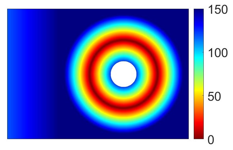
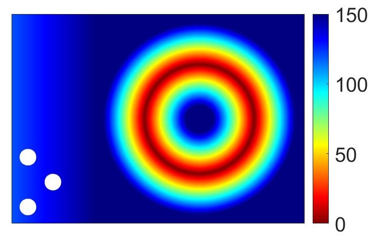
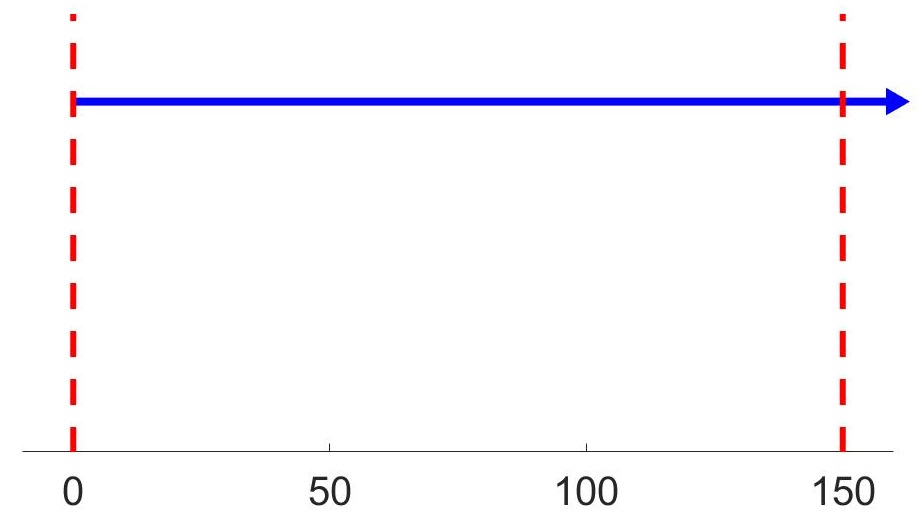
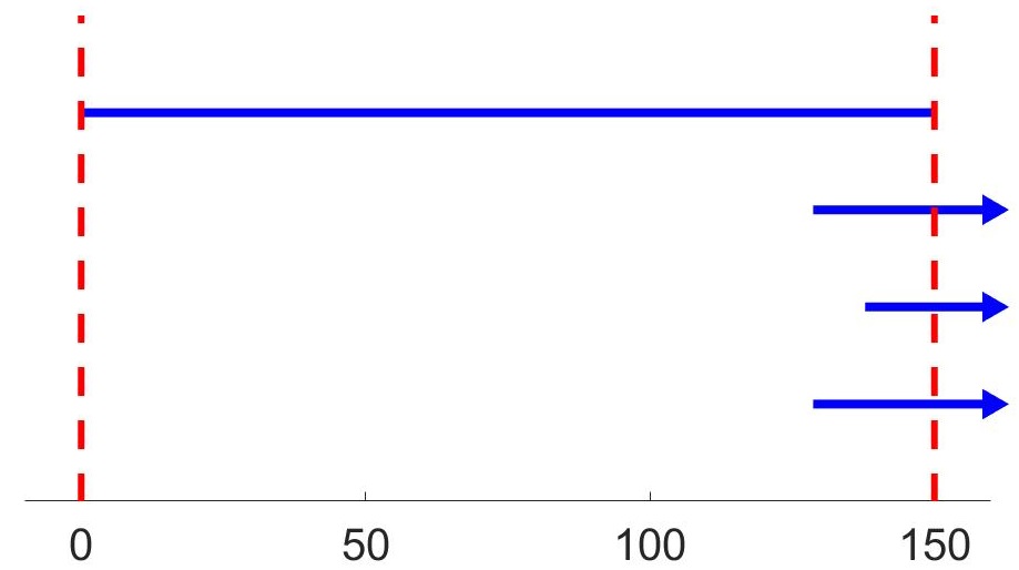
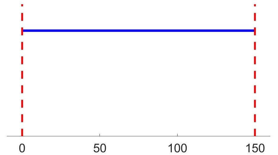
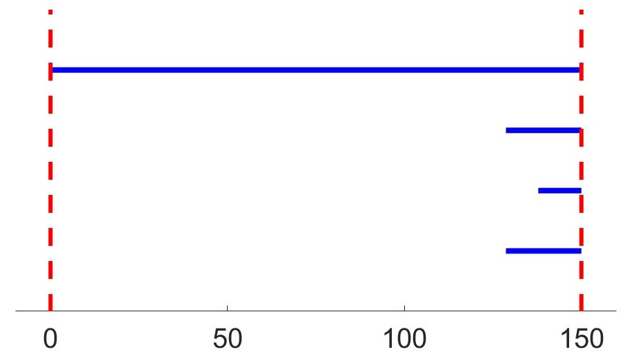
(i)	(ii)	(iii)

Figure 1: The first row shows (i) a “ground truth” image on a rectangle $R$, (ii) the image restricted to $R$ with an open disc removed, and (iii) the image with three noisy holes in its domain. The second row panels display the corresponding barcodes for 1-dimensional persistent homology, calculated using the images as filtering functions. The third row shows the barcodes trimmed at the maximum values of the functions. The arrows indicate bars of infinite length.

As an illustration, we simulate this type of data. Fig. 1 shows signals with very similar shapes, but defined on domains of different homotopy types. The first row shows heat maps of (i) a “ground truth” function defined on a rectangle $R$ and with a circular shape, (ii) the same function restricted to $R$ with an open ball removed that is “encircled” by the signal, and (iii) the same function on $R$ with three noisy holes located in a region where the signal is subdued. The function labeled (i) has global minima along a circle and the center of that circle is a maximum. (Recall that we made the convention that low values correspond to strong signals.) The second row shows the barcodes for 1-dimensional homology obtained from the sublevel set filtrations induced by the images. The barcode for the ground truth image comprises a single bar of finite persistence whose birth-death coordinates $(b,d)$ are the minimum and maximum values of the function, respectively. These values are highlighted by vertical dashed lines. For image (ii), we have a single bar with the same birth coordinate $b$, but of infinite length because the signal wraps around the hole in the domain. For image (iii), we have the original bar of finite length in addition to three infinite bars whose birth coordinates are close to $d$. Thus, in spite of having three signals of very similar shape, the bottleneck distance between any pair of barcodes is infinite. The aforementioned cone construction will have the effect of trimming the barcodes at $d$, as shown on the third row. This yields three barcodes that lie close together with respect to the bottleneck distance because the three noisy bars in (c) are short lived.

It may be instructive to contrast the present approach to persistent homology of metric measure spaces with the treatment by Blumberg et al. [4]. A basic philosophical difference is that whereas we define the persistent homology of a $mm$-space $\mathbb{X}_{\alpha}$ directly via centrality functions and prove stability and consistency results, Blumberg et al. consider the pushforward of the product measure $\otimes_{n}\alpha$ on the $n$-fold product space $X\times\ldots\times X$ to barcode space via the map that associates to a sample of size $n$, the persistent homology of its Vietoris-Rips complex, proving stability and concentration results in this framework. Thus, their approach is based on properties of the distribution of barcodes constructed from independent random draws from the “theoretical” distribution $\alpha$.

As an application, we construct multi-scale persistent homology descriptors for distributions $\alpha$ on a compact Riemannian manifold $M$. We denote the geodesic distance on $M$ by $d_{M}$. Using diffusion distances $d_{t}$, $t>0$, associated with the heat kernel on $M$ (cf. [9, 11]), we obtain metric relaxations of $\mathbb{M}_{\alpha}=(M,d_{M},\alpha)$ via the 1-parameter family $(M,d_{t},\alpha)$ of $mm$-spaces. (We recall the definition of $d_{t}$ in Section 5.) We show that this gives rise to a continuous path of persistence diagrams via the persistent homology of their centrality functions. We employ the framework developed for the topological analysis of $mm$-spaces to prove that this multi-scale topological descriptor is stable with respect to the Wasserstein distance on the space of Borel measures on $(M,d_{M})$.

The rest of the paper is structured as follows. Section 2 develops the aforementioned metric on the space of functional topological spaces and Section 3 proves the stability of persistence homology with respect to this metric. Section 4 addresses stability and consistency of persistent homology of $mm$-spaces. Section 5 is devoted to a multi-scale analysis of distributions on Riemannian manifolds and Section 6 closes the paper with some additional discussion.

2 Functional Topological Spaces

Throughout the paper, we assume that all topological spaces are compact. A functional topological space ($ft$-space) is a triple $\mathbb{X}_{f}=(X,\tau_{X},f)$, where $f\colon X\to\mathbb{R}$ is a continuous function on the topological space $(X,\tau_{X})$. Two $ft$-spaces $\mathbb{X}_{f}$ and $\mathbb{Y}_{g}$ are isomorphic if there is a homeomorphism $h\colon X\to Y$ such that $f=g\circ h$. The collection of isomorphism classes of $ft$-spaces is denoted $\mathscr{F}$. We abuse notation and denote an element of $\mathscr{F}$ as $\mathbb{X}_{f}$. We begin by reviewing a special case of the homotopy type distance $d_{HT}$ of [17] that will be used in our study of functional data. We also introduce a slight variant of $d_{HT}$ that has better properties with respect to the proposed cone construction, as explained in details below. We note that our notation and terminology differ from that of [17].

2.1 The Homotopy Type Distance

A pairing $(\phi,\psi)$ between two topological spaces $(X,\tau_{X})$ and $(Y,\tau_{Y})$ is a pair of continuous mappings $\phi\colon X\to Y$ and $\psi\colon Y\to X$. We denote by $\Pi(X,Y)$ the collection of all such pairings.

Definition 2.1.

Let $h_{0},h_{1}\colon X\to X$ be continuous mappings and $H\colon X\times[0,1]\to X$ a homotopy between $h_{0}$ and $h_{1}$; that is, a continuous mapping such that $H(x,0)=h_{0}(x)$ and $H(x,1)=h_{1}(x)$, $\forall x\in X$. Given $\varepsilon>0$ and a continuous function $f\colon X\to\mathbb{R}$, $H$ is said to be an $\varepsilon$-homotopy from $h_{0}$ to $h_{1}$ over $f$ if

$$(f\circ H)(x,s)\leq(f\circ h_{0})(x)+\varepsilon\,,$$

$\forall x\in X$ and $\forall s\in[0,1]$.

Note that even if $H$ is an $\varepsilon$-homotopy from $h_{0}$ to $h_{1}$ over $f$, the mapping $\overline{H}(x,t)=H(x,1-t)$ may not be an $\varepsilon$-homotopy from $h_{1}$ to $h_{0}$ over $f$.

Definition 2.2.

Let $\mathbb{X}_{f}=(X,\tau_{X},f)$ and $\mathbb{Y}_{g}=(Y,\tau_{Y},g)$ be ft-spaces, $\varepsilon>0$, and $(\phi,\psi)\in\Pi(X,Y)$ a pairing between $\mathbb{X}_{f}$ and $\mathbb{Y}_{g}$.

• $(\phi,\psi)$ is an $\varepsilon$-pairing if $(g\circ\phi)(x)\leq f(x)+\varepsilon$ and $(f\circ\psi)(y)\leq g(y)+\varepsilon$, $\forall x\in X$ and $\forall y\in Y$.

• $(\phi,\psi)$ is a strong $\varepsilon$-pairing if $|(g\circ\phi)(x)-f(x)|\leq\varepsilon$ and $|(f\circ\psi)(y)-g(y)|\leq\varepsilon$, $\forall x\in X$ and $\forall y\in Y$.

Clearly, any strong $\varepsilon$-pairing is an $\varepsilon$-pairing.

Definition 2.3.

Let $\mathbb{X}_{f}$ and $\mathbb{Y}_{g}$ be ft-spaces and $\varepsilon>0$.

• An $\varepsilon$-matching between $\mathbb{X}_{f}$ and $\mathbb{Y}_{g}$ is an $\varepsilon$-pairing $(\phi,\psi)$ that satisfies:

  • there is a $2\varepsilon$-homotopy from $I_{X}$ to $\psi\circ\phi$ over $f$;

  • there is a $2\varepsilon$-homotopy from $I_{Y}$ to $\phi\circ\psi$ over $g$,

  where $I_{X}$ and $I_{Y}$ denote the identity maps of $X$ and $Y$, respectively.

• A strong $\varepsilon$-matching between $\mathbb{X}_{f}$ and $\mathbb{Y}_{g}$ is a strong $\varepsilon$-pairing $(\phi,\psi)$ that satisfies (a) and (b) above.

We use the notation $\mathbb{X}_{f}\sim_{\varepsilon}\mathbb{Y}_{g}$ to indicate that there is an $\varepsilon$-matching between $\mathbb{X}_{f}$ and $\mathbb{Y}_{g}$. The notation $\mathbb{X}_{f}\approx_{\varepsilon}\mathbb{Y}_{g}$ indicates the existence of a strong $\varepsilon$-matching. Note that $\exists\varepsilon>0$ such that $\mathbb{X}_{f}\sim_{\varepsilon}\mathbb{Y}_{g}$ if and only if $X$ and $Y$ are homotopy equivalent. The same statement holds for strong matchings.

Definition 2.4.

Let $\mathbb{X}_{f},\mathbb{Y}_{g}\in\mathscr{F}$ be $ft$-spaces.

• (Frosini et al. [17]) The $d_{HT}$ distance between $\mathbb{X}_{f}$ and $\mathbb{Y}_{g}$ is defined as $d_{HT}(\mathbb{X}_{f},\mathbb{Y}_{g})=\inf\{\varepsilon>0\,|\,\mathbb{X}_{f}\sim_{\varepsilon}\mathbb{Y}_{g}\}$, if $X$ and $Y$ are homotopy equivalent, and $d_{HT}(\mathbb{X}_{f},\mathbb{Y}_{g})=\infty$, otherwise.

• The $\hat{d}_{HT}$ distance is defined as $\hat{d}_{HT}(\mathbb{X}_{f},\mathbb{Y}_{g})=\inf\{\varepsilon>0\,|\,\mathbb{X}_{f}\approx_{\varepsilon}\mathbb{Y}_{g}\}$, if $X$ and $Y$ are homotopy equivalent, and $\hat{d}_{HT}(\mathbb{X}_{f},\mathbb{Y}_{g})=\infty$, otherwise.

Both $d_{HT}$ and $\hat{d}_{HT}$ define extended pseudo-metrics on $\mathscr{F}$, extended meaning that they may attain the value $\infty$. The triangle inequality is easily verified.

2.2 A Cone Construction

As explained in the Introduction, we introduce a cone construction that gives a counterpart to barcode trimming at the $ft$-space level. Let $(X,\tau_{X})$ be a compact topological space. On the product $X\times[0,1]$, consider the equivalence relation generated by $(x,1)\sim(x^{\prime},1)$, $\forall x,x^{\prime}\in X$. The cone on $X$ is the quotient space $C_{X}=X\times[0,1]/\sim$. The quotient topology is denoted $\tau_{C_{X}}$. The cone point is the equivalence class of any $(x,1)$, denoted $\ast_{X}=[(x,1)]$.

Definition 2.5.

Let $\mathbb{X}_{f}\in\mathscr{F}$ be a ft-space. The cone on $\mathbb{X}_{f}$, denoted $\mathbb{C}(\mathbb{X}_{f})$, is the ft-space $(C_{X},\tau_{C_{X}},f^{\ast})$, where $f^{\ast}\colon C_{X}\to\mathbb{R}$ is defined by

$$f^{\ast}([(x,t)])=(1-t)f(x)+tm_{f}\,,$$

for $x\in X$ and $0\leq t\leq 1$. Here, $m_{f}$ is the maximum value of $f$.

Note that for any $a<m_{f}$, the sublevel set $(C_{X})_{a}=(f^{\ast})^{-1}(-\infty,a]$ strong deformation retracts along cone lines to $X_{a}=f^{-1}(-\infty,a]$ and therefore they have the same homology. Moreover, for $a\geq m_{f}$, $(C_{X})_{a}=C_{X}$ which is contractible. Thus, any bar in a barcode whose birth coordinate is close to $m_{f}$ will be short-lived, with the possible exception of a single bar in $H_{0}$.

Define the cone operator  $\mathbb{C}\colon\mathscr{F}\to\mathscr{F}$ by $\mathbb{C}(\mathbb{X}_{f}):=(C_{X},\tau_{C_{X}},f^{\ast})$ and let $r_{\infty}$ and $\hat{r}_{\infty}$ be the pseudo-metrics on $\mathscr{F}$ induced by $d_{HT}$ and $\hat{d}_{HT}$, respectively, under this operator. In other words,

$$r_{\infty}(\mathbb{X}_{f},\mathbb{Y}_{g}):=d_{HT}(\mathbb{C}(\mathbb{X}_{f}),\mathbb{C}(\mathbb{Y}_{g}))\,.$$ (4)

and

$$\hat{r}_{\infty}(\mathbb{X}_{f},\mathbb{Y}_{g}):=\hat{d}_{HT}(\mathbb{C}(\mathbb{X}_{f}),\mathbb{C}(\mathbb{Y}_{g}))\,.$$ (5)

Remark. Since $C_{X}$ and $C_{Y}$ are contractible, thus homotopy equivalent, we have that $r_{\infty}(\mathbb{X}_{f},\mathbb{Y}_{g})<\infty$ and $\hat{r}_{\infty}(\mathbb{X}_{f},\mathbb{Y}_{g})<\infty$, for any $\mathbb{X}_{f},\mathbb{Y}_{g}\in\mathscr{F}$.

One of the drawbacks in directly using the $d_{HT}$ distance in our analysis of functional data is that the cone operator, designed to simplify signals, may in fact increase the $d_{HT}$ distance between $ft$-spaces, making their dissimilarities even more pronounced, as illustrated by the following example.

Example. Let $X=\{(0,0),(1,0)\}$ and $Y=\{(0,y)\,|\,0\leq y\leq 1\}\cup\{(1,0)\}$ with the topology induced by the Euclidean distance in $\mathbb{R}^{2}$. Let $\pi\colon\mathbb{R}^{2}\to\mathbb{R}$ denote projection onto the second coordinate and set $f=\pi|_{X}$ and $g=\pi|_{Y}$, so that $f\equiv 0$. Then, one may show that $d_{HT}(\mathbb{X}_{f},\mathbb{Y}_{g})=0$ and $r_{\infty}(\mathbb{X}_{f},\mathbb{Y}_{g})=d_{HT}(\mathbb{C}(\mathbb{X}_{f}),\mathbb{C}(\mathbb{Y}_{g}))=1$.

In spite of the obvious inequality $d_{HT}(\mathbb{X}_{f},\mathbb{Y}_{g})\leq\hat{d}_{HT}(\mathbb{X}_{f},\mathbb{Y}_{g})$, coning exhibits a much better behavior with respect to $\hat{d}_{HT}$, making it a more natural metric to adopt in some situations. We close this section by showing that the cone operator is non-expansive with respect to $\hat{d}_{HT}$.

Lemma 2.6.

Let $\mathbb{X}_{f}$ and $\mathbb{Y}_{g}$ be ft-spaces. If there is a strong $\varepsilon$-pairing between $\mathbb{X}_{f}$ and $\mathbb{Y}_{g}$, then $|m_{f}-m_{g}|\leq\varepsilon$.

Proof.

Let $(\phi,\psi)$ be such that $|g(\phi(x))-f(x)|\leq\varepsilon$ and $|f(\psi(y))-g(y)|\leq\varepsilon$, for all $x\in X$ and $y\in Y$. Pick $x_{0}\in X$ and $y_{0}\in Y$ that satisfy $m_{f}=f(x_{0})$ and $m_{g}=g(y_{0})$. If $m_{g}\leq m_{f}$, then, $g(\phi(x_{0}))\leq m_{g}\leq m_{f}=f(x_{0})$, so that $|m_{f}-m_{g}|\leq|f(x_{0})-g(\phi(x_{0}))|\leq\varepsilon$. The same argument applies if $m_{f}\leq m_{g}$, proving the lemma. ∎

Given a map $\phi\colon X\to Y$, we refer to $\phi_{c}\colon C_{X}\to C_{Y}$, defined by $\phi_{c}([(x,t)])=[(\phi(x),t)]$, as the cone on $\phi$. We use the notation $\phi_{c}$, instead of $\phi^{\ast}$, to distinguish this construction from the cone on a signal $f$ (see Definition 2.5).

Lemma 2.7.

Let $\mathbb{X}_{f},\mathbb{Y}_{g}\in\mathscr{F}$ and $\varepsilon>0$.

• If $(\phi,\psi)\in\Pi(X,Y)$ is a strong $\varepsilon$-pairing between $\mathbb{X}_{f}$ and $\mathbb{Y}_{g}$, then $(\phi_{c},\psi_{c})\in\Pi(C_{X},C_{Y})$ is a strong $\varepsilon$-pairing between $\mathbb{C}(\mathbb{X}_{f})$ and $\mathbb{C}(\mathbb{Y}_{g})$.

• If $(\phi,\psi)$ is a strong $\varepsilon$-matching between $\mathbb{X}_{f}$ and $\mathbb{Y}_{g}$, then $(\phi_{c},\psi_{c})$ is a strong $\varepsilon$-matching between $\mathbb{C}(\mathbb{X}_{f})$ and $\mathbb{C}(\mathbb{Y}_{g})$.

Proof.

(i) From the definitions of cones and Lemma 2.6, we have that

$$\begin{split}|g^{\ast}(\phi_{c}([(x,t)]))-f^{\ast}([(x,t)])|&\leq(1-t)|(g\circ\phi)(x)-f(x)|+t|m_{f}-m_{g}|\\ &\leq(1-t)\varepsilon+t\varepsilon=\varepsilon\,.\end{split}$$ (6)

Similarly, $|f^{\ast}(\psi_{c}([(x,t)]))-g^{\ast}([(x,t)])|\leq\varepsilon$, proving the claim.

(ii) Let $(\phi,\psi)$ be a strong $\varepsilon$-matching between $\mathbb{X}_{f}$ and $\mathbb{Y}_{g}$. By (i), $(\phi_{c},\psi_{c})$ is a strong $\varepsilon$-pairing, so it suffices to verify the condition on homotopies. Let $H\colon X\times[0,1]\to X$ be a $2\varepsilon$-homotopy from $I_{X}$ to $\psi\circ\phi$ over $f$. We show that $H_{c}\colon C_{X}\times[0,1]\to C_{X}$ defined by $H_{c}([x,t],s)=[H(x,s),t]$ is a $2\varepsilon$-homotopy from $I_{C_{X}}$ to $\psi_{c}\circ\phi_{c}$ over $f^{\ast}$. Indeed,

$$\begin{split}f^{\ast}(H_{c}([x,t],s))&=(1-t)f(H(x,s))+tm_{f}\leq(1-t)(f(x)+2\varepsilon)+tm_{f}\\ &=f^{\ast}([x,t])+2(1-t)\varepsilon\leq f^{\ast}([x,t])+2\varepsilon\,.\end{split}$$ (7)

Similarly, we construct a $2\varepsilon$-homotopy from $I_{C_{Y}}$ to $\phi_{c}\circ\psi_{c}$ over $g^{\ast}$. This concludes the proof. ∎

Proposition 2.8.

The inequality $\hat{r}_{\infty}(\mathbb{X}_{f},\mathbb{Y}_{g})\leq\hat{d}_{HT}(\mathbb{X}_{f},\mathbb{Y}_{g})$ holds for any $\mathbb{X}_{f},\mathbb{Y}_{g}\in\mathscr{F}$.

Proof.

The statement is trivial if $\hat{d}_{HT}(\mathbb{X}_{f},\mathbb{Y}_{g})=\infty$, so we assume that this distance is finite. Let $\varepsilon>\hat{d}_{HT}(\mathbb{X}_{f},\mathbb{Y}_{g})$. Then, there is a strong $\varepsilon$-matching $(\phi,\psi)$ between $\mathbb{X}_{f}$ and $\mathbb{X}_{g}$. By Lemma 2.7 (ii), $(\phi_{c},\psi_{c})$ is a strong $\varepsilon$-matching between $\mathbb{C}(\mathbb{X}_{f})$ and $\mathbb{C}(\mathbb{Y}_{g})$. Thus $\hat{r}_{\infty}(\mathbb{X}_{f},\mathbb{Y}_{g})\leq\varepsilon$. Taking infimum over $\varepsilon>\hat{d}_{HT}(\mathbb{X}_{f},\mathbb{Y}_{g})$, the claim follows. ∎

3 Topology of Functional Spaces

We briefly recall the definitions of persistence modules over $(\mathbb{R},\leq)$ and interleaving distance between two persistence modules. For more details, we refer the reader to [7, 22]. We regard $(\mathbb{R},\leq)$ as a category $\mathscr{R}$ whose objects are the points $a\in\mathbb{R}$ with a single morphism $a\to b$ if $a\leq b$ and none otherwise. A persistence module $\mathbb{V}$ (over a fixed field $\mathbb{F}$) is a functor $\mathcal{F}$ from $\mathscr{R}$ to the category of vector spaces over $\mathbb{F}$. We use the notation $V_{a}:=\mathcal{F}(a)$ for the vector space over $a\in\mathbb{R}$. For $a\leq b$, we write $\nu_{a}^{b}\colon V_{a}\to V_{b}$ for the linear mapping associated with the morphism $a\to b$.

Let $\mathbb{V}=\{V_{a},\nu_{a}^{b}\}$ and $\mathbb{W}=\{W_{a},\omega_{a}^{b}\}$ be persistence modules and $\varepsilon>0$. A morphism $\Phi\colon\mathbb{V}\to\mathbb{W}$ of degree $\varepsilon$ is a collection of linear mappings $\phi_{a}\colon V_{a}\to W_{a+\varepsilon}$, $a\in\mathbb{R}$, satisfying $\omega_{a+\varepsilon}^{a+r+\varepsilon}\circ\phi_{a}=\phi_{a+r}\circ\nu_{a}^{a+r}$, for any $a\in\mathbb{R}$ and $r\geq 0$. An $\varepsilon$-interleaving between $\mathbb{V}$ and $\mathbb{W}$ is a pair $\Phi\colon\mathbb{V}\to\mathbb{W}$ and $\Psi\colon\mathbb{W}\to\mathbb{V}$ of morphisms of degree $\varepsilon$ satisfying $\psi_{a+\varepsilon}\circ\phi_{a}=\nu_{a}^{a+2\varepsilon}$ and $\phi_{a+\varepsilon}\circ\psi_{a}=\omega_{a}^{a+2\varepsilon}$, $\forall a\in\mathbb{R}$. We write $\mathbb{V}\sim_{\varepsilon}\mathbb{W}$ to indicate that there is an $\varepsilon$-interleaving between the two persistence modules. The interleaving distance $d_{I}$ is defined as:

• $d_{I}(\mathbb{V},\mathbb{W})=\infty$, if no interleaving exists;

• $d_{I}(\mathbb{V},\mathbb{W})=\inf\{\varepsilon>0\,|\,\mathbb{V}\sim_{\varepsilon}\mathbb{W}\}$, otherwise.

A persistence module $\mathbb{V}$ is tame if $\nu_{a}^{b}$ has finite rank, for any $a<b$. There is a well-defined persistence diagram (or barcode), denoted $PD(\mathbb{V})$, associated with any tame $\mathbb{V}$ and the Isomorphism Theorem for persistence modules states that

$$d_{b}(PD(\mathbb{V}),PD(\mathbb{W}))=d_{I}(\mathbb{V},\mathbb{W})\,,$$ (8)

if $\mathbb{V}$ and $\mathbb{W}$ are tame, where $d_{b}$ denotes bottleneck distance [8, 10].

3.1 Stability of Persistent Homology

Let $\mathbb{X}_{f}\in\mathscr{F}$ be an $ft$-space. For $a\in\mathbb{R}$, let $X_{a}=f^{-1}(-\infty,a]$ be the corresponding sub-level set of $f$. Clearly, $X_{a}\subseteq X_{b}$, if $a\leq b$, and $\cup_{a\in\mathbb{R}}X_{a}=X$. Thus, the sub-level sets of $f$ induce a filtration of $X$ by closed subsets, which may be viewed as a functor from $\mathcal{R}$ to the category of topological spaces and continuous mappings. Composition with the $i$-dimensional homology functor (with coefficients in $\mathbb{F}$) yields a persistence module, which we denote by $\mathbb{H}_{i}(\mathbb{X}_{f})$. The vector space over $a\in\mathbb{R}$ is $H_{i}(X_{a})$ and the morphism $\iota_{a}^{b}\colon H_{i}(X_{a})\to H_{i}(X_{b})$, $a\leq b$, is the homomorphism on homology induced by inclusion.

A stability theorem for persistent homology of $ft$-spaces has been proven in [17], but we include a proof for the one-parameter persistence case needed in this paper.

Theorem 3.1 (Frosini et al. [17]).

Let $\mathbb{X}_{f}$ and $\mathbb{Y}_{g}$ be functional topological spaces. Then,

$$d_{I}(\mathbb{H}_{i}(\mathbb{X}_{f}),\mathbb{H}_{i}(\mathbb{Y}_{g}))\leq d_{HT}(\mathbb{X}_{f},\mathbb{Y}_{g})\,.$$

Proof.

It suffices to consider the case $d_{HT}(\mathbb{X}_{f},\mathbb{Y}_{g})<\infty$. Let $(\phi,\psi)\in\Pi(X,Y)$ be an $\varepsilon$-matching between $\mathbb{X}_{f}$ and $\mathbb{Y}_{g}$. For any $a\in\mathbb{R}$, condition (i) in Definition 2.2 ensures that $\phi(X_{a})\subseteq Y_{a+\varepsilon}$. Thus, $\phi$ induces a mapping $\phi_{a}\colon X_{a}\to Y_{a+\varepsilon}$. Similarly, $\psi$ induces mappings $\psi_{a}\colon Y_{a}\to X_{a+\varepsilon}$. Condition (a) in Definition 2.3(i) implies that $\psi_{a+\varepsilon}\circ\phi_{a}\colon X_{a}\to X_{a+2\varepsilon}$ is homotopic to the inclusion map $X_{a}\hookrightarrow X_{a+2\varepsilon}$. Analogously, $\phi_{a+\varepsilon}\circ\psi_{a}\colon Y_{a}\to Y_{a+2\varepsilon}$ is homotopic to the inclusion map $Y_{a}\hookrightarrow Y_{a+2\varepsilon}$. Thus, the homomorphisms on homology induced by $\phi_{a}$ and $\psi_{a}$, $a\in\mathbb{R}$, yield an $\varepsilon$-interleaving between $\mathbb{H}_{i}(\mathbb{X}_{f})$ and $\mathbb{H}_{i}(\mathbb{Y}_{g})$. This implies that $d_{I}(\mathbb{H}_{i}(\mathbb{X}_{f}),\mathbb{H}_{i}(\mathbb{Y}_{g}))\leq\varepsilon$. Taking infimum over $\varepsilon>d_{HT}(\mathbb{X}_{f},\mathbb{Y}_{g})$, the result follows. ∎

Corollary 3.2.

Let $\mathbb{X}_{f}$ and $\mathbb{Y}_{g}$ be functional topological spaces. Then,

$$d_{I}(\mathbb{H}^{\ast}_{i}(\mathbb{X}_{f}),\mathbb{H}^{\ast}_{i}(\mathbb{Y}_{g}))\leq r_{\infty}(\mathbb{X}_{f},\mathbb{Y}_{g})\leq\hat{r}_{\infty}(\mathbb{X}_{f},\mathbb{Y}_{g})\leq\hat{d}_{HT}(\mathbb{X}_{f},\mathbb{Y}_{g})\,,$$

where $\mathbb{H}^{\ast}_{i}(\mathbb{X}_{f})=\mathbb{H}_{i}(\mathbb{C}(\mathbb{X}_{f}))$ and $\mathbb{H}^{\ast}_{i}(\mathbb{Y}_{g})=\mathbb{H}_{i}(\mathbb{C}(\mathbb{Y}_{g}))$.

Proof.

The first inequality follows from Theorem 3.1 and (4). The second inequality is a direct consequence of the definition of the metrics $r_{\infty}$ and $\hat{r}_{\infty}$. The third inequality was proven in Proposition 2.8. ∎

If $(X,\tau_{X})$ is a triangulable space, then $\mathbb{H}^{\ast}_{i}(\mathbb{X}_{f})$ is tame (cf. [8, 10]) so that there is a well-defined persistence diagram $PD_{i}^{\ast}(\mathbb{X}_{\alpha})$ associated with $\mathbb{H}^{\ast}_{i}(\mathbb{X}_{f})$.

Corollary 3.3.

Let $\mathbb{X}_{f}$ and $\mathbb{Y}_{g}$ be triangulable ft-spaces and $i\geq 0$ be an integer. Then,

$$d_{B}(PD_{i}^{\ast}(\mathbb{X}_{f}),PD_{i}^{\ast}(\mathbb{Y}_{g})\leq r_{\infty}(\mathbb{X}_{f},\mathbb{Y}_{g})\leq\hat{r}_{\infty}(\mathbb{X}_{f},\mathbb{Y}_{g})\leq\hat{d}_{HT}(\mathbb{X}_{f},\mathbb{Y}_{g})\,.$$

Proof.

This follows from Corollary 3.2 and (8). ∎

3.2 Effect of Coning on Persistent Homology

As explained in the Introduction, one of the practical motivations for coning functional data is the truncation effect it has on persistent homology of their sublevel set filtrations. Here, we show more formally that this is indeed the effect of coning an $ft$-space.

Definition 3.4.

Let $\mathbb{V}=\{V_{a},\nu_{a}^{b}\}$ be a persistence module and $r\in\mathbb{R}$. The $r$-truncation of $\mathbb{V}$ is defined as the persistence module $T_{r}(\mathbb{V}):=\{\overline{V}_{a},\overline{\nu}_{a}^{b}\}$, where

$$\overline{V}_{a}=\begin{cases}V_{a}&\text{if $a<r$;}\\ 0&\text{if $a\geq r$;}\\ \end{cases}\qquad\text{and}\qquad\overline{\nu}_{a}^{b}=\begin{cases}\nu_{a}^{b}&\text{if $b<r$;}\\ 0&\text{if $b\geq r$.}\\ \end{cases}$$

Let $\mathbb{X}_{f}$ be an $ft$-space and $m=\min f$. We denote by $\mathbb{P}_{g}$ the $ft$-space where $P=\{p\}$ is a one-point space and $g\colon P\to\mathbb{R}$ is given by $g(p)=m$. By the definition of $g$, the (constant) maps $\phi_{1}\colon X\to P$ and $\phi_{2}\colon C_{X}\to P$ have the property that the sublevel sets of $f$, $f^{\ast}$ and $g$ satisfy $\phi_{1}(X_{a})\subseteq P_{a}$ and $\phi_{2}((C_{X})_{a})\subseteq P_{a}$, $\forall a\in\mathbb{R}$. It is simple to verify that, for each $i\geq 0$, $\phi_{1}$ and $\phi_{2}$ induce homomorphisms $\phi_{1\ast}\colon\mathbb{H}_{i}(\mathbb{X}_{f})\to\mathbb{H}_{i}(\mathbb{P}_{g})$ and $\phi_{2\ast}\colon\mathbb{H}^{\ast}_{i}(\mathbb{X}_{f})\to\mathbb{H}_{i}(\mathbb{P}_{g})$ of persistence modules. Note that $\mathbb{H}_{0}(\mathbb{P}_{g})$ is isomorphic to the interval module $\mathbb{I}_{m}^{\infty}$ associated with the interval $[m,\infty)$, and $\mathbb{H}_{i}(\mathbb{P}_{g})=0$ for $i>0$. The kernels of $\phi_{1\ast}$ and $\phi_{2\ast}$ give persistence submodules $\widetilde{\mathbb{H}}_{i}(\mathbb{X}_{f}):=\ker(\phi_{1\ast})$ and $\widetilde{\mathbb{H}}^{\ast}_{i}(\mathbb{X}_{f}):=\ker(\phi_{2\ast})$ of $\mathbb{H}_{i}(\mathbb{X}_{f})$ and $\mathbb{H}^{\ast}_{i}(\mathbb{X}_{f})$, respectively, which yield direct sum decompositions

$$\mathbb{H}_{i}(\mathbb{X}_{f})\cong\widetilde{\mathbb{H}}_{i}(\mathbb{X}_{f})\oplus\mathbb{H}_{i}(\mathbb{P}_{g})\quad\text{and}\quad\mathbb{H}^{\ast}_{i}(\mathbb{X}_{f})\cong\widetilde{\mathbb{H}}^{\ast}_{i}(\mathbb{X}_{f})\oplus\mathbb{H}_{i}(\mathbb{P}_{g})\,.$$ (9)

(These decompositions are non-trivial only for the case when $i=0$ since $\mathbb{H}_{i}(\mathbb{P}_{g})=0$ for $i>0$.) One may construct such isomorphisms by splitting the homomorphisms $\phi_{1\ast}$ and $\phi_{2\ast}$, as follows. Pick $x_{0}\in X$ such that $f(x_{0})=m$ and let $\psi_{1}\colon P\to X$ and $\psi_{2}\colon P\to C_{X}$ be given by $\psi_{1}(p)=x_{0}$ and $\psi_{2}(p)=[(x_{0},0)]$. Then, the induced homomorphisms $\psi_{1\ast}$ and $\psi_{2\ast}$ on persistence modules are well defined and split $\phi_{1\ast}$ and $\phi_{2\ast}$, as desired. As usual, the splitting is not natural.

Proposition 3.5.

Let $i\geq 0$ be an integer, $\mathbb{X}_{f}\in\mathscr{F}$, and $m_{f}=\max f$. Then, $\widetilde{\mathbb{H}}^{\ast}_{i}(\mathbb{X}_{f})=\widetilde{\mathbb{H}}_{i}(\mathbb{C}(\mathbb{X}_{f}))$ is isomorphic to $T_{m_{f}}(\widetilde{\mathbb{H}}_{i}(\mathbb{X}_{f}))$.

Proof.

Let $\iota\colon X\hookrightarrow C_{X}$ be the inclusion $x\mapsto[(x,0)]$. Then, the sublevel sets of $f$ and $f^{\ast}$ satisfy $\iota(X_{a})\subseteq(C_{X})_{a}$, $\forall a\in\mathbb{R}$, and $\iota$ induces a homomorphism $\iota_{\ast}\colon\mathbb{H}_{i}(\mathbb{X}_{f})\to\mathbb{H}_{i}(\mathbb{C}(\mathbb{X}_{f}))$. The commutativity of the diagram

(10)

for any $a\in\mathbb{R}$, implies that $\iota_{\ast}(\widetilde{\mathbb{H}}_{i}(\mathbb{X}_{f}))\subseteq\widetilde{\mathbb{H}}_{i}(\mathbb{C}(\mathbb{X}_{f}))$. Since $\iota$ induces a homotopy equivalence between $X_{a}$ and $(C_{X})_{a}$, for $a<m_{f}$, $\iota_{\ast}$ induces an isomorphism $\iota_{\ast}\colon\widetilde{H}_{i}(X_{a})\to\widetilde{H}_{i}((C_{X})_{a})$, for $a<m_{f}$. Combining this with the fact that the reduced homology of $(C_{X})_{a}$ is trivial for $a\geq m_{f}$, we conclude that $\iota_{\ast}$ induces an isomorphism between $\widetilde{\mathbb{H}}_{i}(\mathbb{C}(\mathbb{X}_{f}))$ and $T_{m_{f}}(\widetilde{\mathbb{H}}_{i}(\mathbb{X}_{f}))$, as claimed. ∎

Corollary 3.6.

Suppose that $\mathbb{X}_{f}\in\mathscr{F}$ with $(X,\tau_{X})$ triangulable and let $m=\min f$ and $m_{f}=\max f$. For any integer $i\geq 0$, let $I_{\lambda}\subset\mathbb{R}$, $\lambda\in\Lambda_{i}$, be intervals such that the corresponding interval modules $\mathbb{I}_{\lambda}$ yield a decomposition $\widetilde{\mathbb{H}}_{i}(\mathbb{X}_{f})=\bigoplus_{\lambda\in\Lambda_{i}}\mathbb{I}_{\lambda}$. Then,

• $\mathbb{H}_{0}^{\ast}(\mathbb{X}_{f})\cong\mathbb{I}_{m}^{\infty}\oplus\bigoplus_{\lambda\in\Lambda_{0}}\mathbb{I}_{\lambda}^{m_{f}}$;

• $\mathbb{H}_{i}^{\ast}(\mathbb{X}_{f})\cong\bigoplus_{\lambda\in\Lambda_{i}}\mathbb{I}_{\lambda}^{m_{f}}$, for $i>0$.

Here, $\mathbb{I}_{\lambda}^{m_{f}}$ and $\mathbb{I}_{m}^{\infty}$ are the interval modules associated with $I^{m_{f}}_{\lambda}=I_{\lambda}\cap(-\infty,m_{f})$ and $I_{m}^{\infty}=[m,\infty)$, respectively. We make the convention that $\mathbb{I}_{\lambda}^{m_{f}}$ is trivial if $I^{m_{f}}_{\lambda}=\emptyset$.

Proof.

This is an immediate consequence of (9) and Proposition 3.5. ∎

4 Metric Measure Spaces

A metric measure space ($mm$-space) is a triple $\mathbb{X}_{\alpha}=(X,d_{X},\alpha)$, where $\mathbb{X}=(X,d_{X})$ is a metric space and $\alpha$ is a Borel probability measure on $X$. We assume that all $mm$-spaces are compact. Two $mm$-spaces $\mathbb{X}_{\alpha}=(X,d_{X},\alpha)$ and $\mathbb{Y}_{\beta}=(Y,d_{Y},\beta)$ are isomorphic if there is an isometry $h\colon X\to Y$ such that $h_{\ast}(\alpha)=\beta$. We denote by $\mathscr{M}$ the collection of isomorphism classes of compact $mm$-spaces, but often refer to $\mathbb{X}_{\alpha}$ as an element of $\mathscr{M}$. We begin by equipping $\mathscr{M}$ with a pseudo-metric that let us address stability of persistence diagrams that seek to emphasize the shape of regions rich in probability mass, downplaying the geometry of regions that are not central to the distribution, as characterized by larger values of the centrality function.

4.1 A Metric on $\boldsymbol{\mathscr{M}}$

To motivate our definition of a (pseudo) metric on $\mathscr{M}$ that is well suited to the study of stability of the topology of centrality functions, we briefly digress on well known metrics of related nature. Metrics such as the Gromov-Hausdorff distance $d_{GH}$ between compact metric spaces and the Gromov-Wasserstein distance $d_{GW,p}$ beween metric measure spaces may be defined via measures of distortion of correspondences between the relevant spaces. “Hard” correspondences given by a relation between two metric domains may be used to define $d_{GH}$, whereas “soft” correspondences given by couplings of probability measures may be used for $d_{GW,p}$. More precisely, let $\mathbb{X}=(X,d_{X})$ and $\mathbb{Y}=(Y,d_{Y})$ be compact metric spaces. A correspondence $R$ between $X$ and $Y$ is a subset $R\subset X\times Y$ such that $\pi_{X}(R)=X$ and $\pi_{Y}(R)=Y$. The distortion of $R$ is given by

$$D(R):=\sup_{\tiny\begin{matrix}(x,y)\in R\\ (x^{\prime},y^{\prime})\in R\end{matrix}}|d_{X}(x,x^{\prime})-d_{Y}(y,y^{\prime})|\,,$$ (11)

and the Gromov-Hausdorff distance may be defined as

$$d_{GH}(\mathbb{X},\mathbb{Y}):=\frac{1}{2}\inf_{\tiny R}D(R)\,,$$ (12)

where the infimum is taken over all correspondences $R$ between $X$ and $Y$ [19]. Similarly, a coupling between $\mathbb{X}_{\alpha}$ and $\mathbb{Y}_{\beta}$ is a Borel probability measure $\mu$ on $X\times Y$ that marginalizes to $\alpha$ and $\beta$, respectively. In other words, $(\pi_{X})_{\ast}(\mu)=\alpha$ and $(\pi_{Y})_{\ast}(\mu)=\beta$. The collection of all such couplings is denoted $\Gamma(\mathbb{X}_{\alpha},\mathbb{Y}_{\beta})$. For $p\geq 1$, the $p$-distortion of a coupling $\mu$ is defined as

$$D_{p}(\mu):=\left(\int\int|d_{X}(x,x^{\prime})-d_{Y}(y,y^{\prime})|^{p}\,d\mu(x,y)d\mu(x^{\prime},y^{\prime})\right)^{1/p}$$ (13)

and

$$d_{GW,p}(\mathbb{X}_{\alpha},\mathbb{Y}_{\beta}):=\inf_{\mu}D_{p}(\mu),$$ (14)

with the infimum taken over all $\mu\in\Gamma(\mathbb{X}_{\alpha},\mathbb{Y}_{\beta})$ (cf. [23]). In both definitions, a single correspondence or coupling is used for both $(x,y)$ and $(x^{\prime},y^{\prime})$. We employ a hybrid version that combines a hard correspondence for $(x,y)$ and a soft correspondence for $(x^{\prime},y^{\prime})$, except that the hard correspondence will be given by a pair of continuous mappings between metric spaces rather than a relation. As a first step toward this goal, for each coupling $\mu\in\Gamma(\mathbb{X}_{\alpha},\mathbb{Y}_{\beta})$, we define a (pseudo) metric $d_{p,\mu}$ on the disjoint union $X\sqcup Y$, as follows.

On the $X$ component, we define a pseudo-metric $d_{p,\alpha}$ by mapping $X$ to the function space $\mathbb{L}_{p}(\mathbb{X}_{\alpha})$ and taking the induced metric, as follows. Let $K\colon(X,d_{X})\to\mathbb{L}_{p}(\mathbb{X}_{\alpha})$, $x\mapsto K_{x}$, be given by $K_{x}(x^{\prime})=d_{X}(x,x^{\prime})$. Then, $d_{p,\alpha}$ is the (pseudo) metric on $X$ induced by the norm $\|\cdot\|_{p,\alpha}$ under this map. In other words,

$$\begin{split}d_{p,\alpha}(x_{1},x_{2})=\left(\int_{X}|d_{X}(x_{1},x^{\prime})-d_{X}(x_{2},x^{\prime})|^{p}\,d\alpha(x^{\prime})\right)^{1/p}\,.\end{split}$$ (15)

Note that, since $\mu$ has $\alpha$ as marginal, we have

$$\begin{split}d_{p,\alpha}(x_{1},x_{2})&=\left(\int_{X\times Y}|d_{X}(x_{1},x^{\prime})-d_{X}(x_{2},x^{\prime})|^{p}\,d\mu(x^{\prime},y^{\prime})\right)^{1/p}\\ &=\|K_{x_{1}}-K_{x_{2}}\|_{p,\mu}\,.\end{split}$$ (16)

Similarly, define $d_{p,\beta}$ on the $Y$ component. Using the coupling, we define $d_{p,\mu}$ on the disjoint union $X\sqcup Y$ that restricts to $d_{p,\alpha}$ and $d_{p,\beta}$ on $X$ and $Y$, respectively. The distance between $x\in X$ and $y\in Y$ is given by

$$\begin{split}d_{p,\mu}(x,y)&=\left(\int_{X\times Y}|d_{X}(x,x^{\prime})-d_{Y}(y,y^{\prime})|^{p}\,d\mu(x^{\prime},y^{\prime})\right)^{1/p}\\ &=\|K_{x}-K_{y}\|_{p,\mu}\end{split}$$ (17)

Proposition 4.1.

For any $p\geq 1$ and $\mu\in\Gamma(\mathbb{X}_{\alpha},\mathbb{Y}_{\beta})$, the distance $d_{p,\mu}$ defines a pseudo-metric on $X\sqcup Y$.

Proof.

The distance $d_{p,\mu}$ is clearly symmetric, so it suffices to verify the triangle inequality, which is valid because $d_{p,\mu}$ is induced by an $\mathbb{L}_{p}$-norm. Indeed, suppose $x_{1},x_{2}\in X$ and $y\in Y$. Then, by (16), (17) and the Minkowski inequality, we have that

$$\begin{split}d_{p,\mu}(x_{1},y)=\|K_{x_{1}}-K_{y}\|_{p,\mu}&\leq\|K_{x_{1}}-K_{x_{2}}\|_{p,\mu}+\|K_{x_{2}}-K_{y}\|_{p,\mu}\\ &=d_{p,\mu}(x_{1},x_{2})+d_{p,\mu}(x_{2},y)\,.\end{split}$$ (18)

Other cases may be verified in an analogous manner. ∎

Definition 4.2.

Let $\mathbb{X}_{\alpha},\mathbb{Y}_{\beta}$ be $mm$-spaces, $(\phi,\psi)\in\Pi(X,Y)$ a pairing between $(X,d_{X})$ and $(Y,d_{Y})$, and $\mu\in\Gamma(\mathbb{X}_{\alpha},\mathbb{Y}_{\beta})$ a coupling. We define three distortions associated with $\phi$, $\psi$ and $\mu$:

• $D(\phi,\mu):=\sup_{x\in X}d_{p,\mu}(x,\phi(x))$ and $D(\psi,\mu):=\sup_{y\in Y}d_{p,\mu}(\psi(y),y)$;

• $D(\phi,\psi,\mu):=\max\{D(\phi,\mu),D(\psi,\mu)\}$.

Definition 4.3.

Let $\mathbb{X}_{\alpha},\mathbb{Y}_{\beta}$ be $mm$-spaces, $\varepsilon>0$ and $p\geq 1$. An $\varepsilon$-matching (of order $p$) between $\mathbb{X}_{\alpha}$ and $\mathbb{Y}_{\beta}$ is a pairing $(\phi,\psi)\in\Pi(X,Y)$ and a coupling $\mu\in\Gamma(\alpha,\beta)$ such that:

• $D(\phi,\psi,\mu)\leq\varepsilon$;

• There is a $2\varepsilon$-homotopy from the identity map $I_{C_{X}}$ to $\psi_{c}\circ\phi_{c}\colon C_{X}\to C_{X}$ over $\sigma^{\ast}_{p,\mathbb{X}_{\alpha}}\colon C_{X}\to\mathbb{R}$;

• There is a $2\varepsilon$-homotopy from the identity map $I_{C_{Y}}$ to $\phi_{c}\circ\psi_{c}\colon C_{Y}\to C_{Y}$ over $\sigma^{\ast}_{p,\mathbb{Y}_{\beta}}\colon C_{Y}\to\mathbb{R}$.

We write $\mathbb{X}_{\alpha}\sim_{\varepsilon}\mathbb{Y}_{\beta}$ to indicate that there is an $\varepsilon$-matching between $\mathbb{X}_{\alpha}$ and $\mathbb{Y}_{\beta}$ and define

$$\delta_{p}(\mathbb{X}_{\alpha},\mathbb{Y}_{\beta})=\inf\{\varepsilon\,|\,\mathbb{X}_{\alpha}\sim_{\varepsilon}\mathbb{Y}_{\beta}\}\,.$$ (19)

For any $p\geq 1$, $\delta_{p}$ induces a pseudo-metric on $\mathscr{M}$.

The next lemma shows that, for probability measures defined on the same metric space, the Wasserstein distance gives an upper bound for $\delta_{p}$. We denote the collection of all Borel probability measures on a compact metric space $(X,d_{X})$ by $\mathcal{P}(X)$ and the Wasserstein metric of order $p\geq 1$ on $\mathcal{P}(X)$ by $w_{p}$.

Lemma 4.4.

For any $\alpha,\beta\in\mathcal{P}(X)$, $\delta_{p}(\mathbb{X}_{\alpha},\mathbb{X}_{\beta})\leq w_{p}(\alpha,\beta)$.

Proof.

Let $\mu\in\Gamma(\alpha,\beta)$ be a coupling that realizes $w_{p}(\alpha,\beta)$; that is,

$$\left(\int_{X}d^{p}_{X}(x,x^{\prime})\,d\mu(x,x^{\prime})\right)^{1/p}=w_{p}(\alpha,\beta)\,.$$ (20)

By the triangle inequality, the trivial pairing $(\phi,\psi)=(I_{X},I_{X})$ between $\mathbb{X}_{\alpha}$ and $\mathbb{X}_{\beta}$ satisfies

$$\begin{split}d_{p,\mu}(x,\phi(x))&=\left(\int_{X\times X}|d_{X}(x,x_{1})-d_{X}(x,x_{2})|^{p}\,d\mu(x_{1},x_{2})\right)^{1/p}\\ &\leq\left(\int_{X\times X}d^{p}_{X}(x_{1},x_{2})\,d\mu(x_{1},x_{2})\right)^{1/p}=w_{p}(\alpha,\beta)\,.\end{split}$$ (21)

Thus, condition (i) in Definition 4.3 is satisfied for $\varepsilon=w_{p}(\alpha,\beta)$. Conditions (ii) and (iii) are trivially satisfied by this pairing. Therefore, $\delta_{p}(\mathbb{X}_{\alpha},\mathbb{X}_{\beta})\leq w_{p}(\alpha,\beta)$. ∎

4.2 Stability and Consistency

One of our main goals is to study the shape of a $mm$-space $\mathbb{X}_{\alpha}$ via the persistent homology of the sublevel set filtration of $C_{X}$ induced by the cone on the centrality function. As an intermediate step, we map $(\mathscr{M},\delta_{p})$ to the functional space $(\mathscr{F},r_{\infty})$. For $p\geq 1$, let $\Theta_{p}\colon\mathscr{M}\to\mathscr{F}$ be the mapping given by

$$\Theta_{p}(\mathbb{X}_{\alpha})=(X,\tau_{X},\sigma_{p,\mathbb{X}_{\alpha}})\,,$$ (22)

where $\tau_{X}$ is the topology underlying the metric space $(X,d_{X})$ and $\sigma_{p,\mathbb{X}_{\alpha}}$ is the $p$-centrality function of $\mathbb{X}_{\alpha}$. We denote by $\mathbb{H}^{\ast}_{i}(\Theta_{p}(\mathbb{X}_{\alpha}))$ the persistence module for $i$-dimensional homology of the cone $\mathbb{C}(\Theta_{p}(\mathbb{X}_{\alpha}))$. If $(X,d_{X})$ is triangulable, there is a well defined persistence diagram $PD^{\ast}_{i}(\Theta_{p}(\mathbb{X}_{\alpha}))$ associated with this persistence module.

We begin our investigation of stability by showing that $p$-centrality is stable with respect to $\delta_{p}$. To simplify notation, we write

$$\Theta_{p}(\mathbb{X}_{\alpha})=\mathbb{X}_{\alpha,p}\,.$$ (23)

Proposition 4.5.

Let $p\geq 1$. If $\mathbb{X}_{\alpha},\mathbb{Y}_{\beta}\in\mathscr{M}$ are $mm$-spaces, then

$$\hat{r}_{\infty}(\mathbb{X}_{\alpha,p},\mathbb{Y}_{\beta,p})=\hat{d}_{HT}(\mathbb{C}(\mathbb{X}_{\alpha,p}),\mathbb{C}(\mathbb{Y}_{\beta,p}))\leq\delta_{p}(\mathbb{X}_{\alpha},\mathbb{Y}_{\beta})\,.$$

Proof.

Fix $\varepsilon>\delta_{p}(\mathbb{X}_{\alpha},\mathbb{Y}_{\beta})$ and let $(\phi,\psi)\in\Pi(X,Y)$ and $\mu\in\Gamma(\alpha,\beta)$ induce an $\varepsilon$-matching between $\mathbb{X}_{\alpha}$ and $\mathbb{Y}_{\beta}$. We show that $(\phi_{c},\psi_{c})$ is a strong $\varepsilon$-matching between the cones on the $ft$-spaces $\mathbb{X}_{\alpha,p}$ and $\mathbb{Y}_{\beta,p}$. Write

$$\sigma_{p,\mathbb{X}_{\alpha}}(x)=\left(\int_{X}d_{X}^{p}(x,x^{\prime})\,d\alpha(x^{\prime})\right)^{1/p}=\left(\int_{X\times Y}d_{X}^{p}(x,x^{\prime})\,d\mu(x^{\prime},y^{\prime})\right)^{1/p}$$ (24)

and

$$\sigma_{p,\mathbb{Y}_{\beta}}(y)=\left(\int_{Y}d_{Y}^{p}(y,y^{\prime})\,d\beta(y^{\prime})\right)^{1/p}=\left(\int_{X\times Y}d_{Y}^{p}(y,y^{\prime})\,d\mu(x^{\prime},y^{\prime})\right)^{1/p}\,.$$ (25)

By (24), (25) and the Minkowski inequality, we have that

$$\begin{split}|(\sigma_{p,\mathbb{Y}_{\beta}}\circ\phi)(x)-\sigma_{p,\mathbb{X}_{\alpha}}(x)|&\leq\left(\int_{X\times Y}|d_{X}(x,x^{\prime})-d_{Y}(\phi(x),y^{\prime})|^{p}\,d\mu(x^{\prime},y^{\prime})\right)^{1/p}\\ &=d_{p,\mu}(x,\phi(x))\leq\varepsilon\,,\end{split}$$ (26)

$\forall x\in X$. Similarly, $|(\sigma_{p,\mathbb{X}_{\alpha}}\circ\psi)(y)-\sigma_{p,\mathbb{Y}_{\beta}}(y)|\leq\varepsilon$. Thus, $(\phi,\psi)$ is a strong $\varepsilon$-pairing between $\mathbb{X}_{\sigma_{p,\mathbb{X}_{\alpha}}}$ and $\mathbb{Y}_{\sigma_{p,\mathbb{Y}_{\beta}}}$. By Lemma 2.7(i), $(\phi_{c},\psi_{c})$ is a strong $\varepsilon$-pairing between the cones on $\mathbb{X}_{\alpha,p}$ and $\mathbb{Y}_{\beta,p}$. Since $(\phi,\psi)$ and $\mu$ induce an $\varepsilon$-matching between $\mathbb{X}_{\alpha}$ and $\mathbb{Y}_{\beta}$, conditions (a) and (b) in Definition 2.3 are satisfied by $(\phi_{c},\psi_{c})$. Hence,

$$\hat{r}_{\infty}(\mathbb{X}_{\alpha,p},\mathbb{Y}_{\beta,p})=\hat{d}_{HT}(\mathbb{C}(\mathbb{X}_{\alpha,p}),\mathbb{C}(\mathbb{Y}_{\beta,p}))\leq\varepsilon\,.$$ (27)

Taking infimum over $\varepsilon$-matchings, the result follows. ∎

Theorem 4.6 (Stability of Persistent Homology).

Let $p\geq 1$ and $\mathbb{X}_{\alpha},\mathbb{Y}_{\beta}\in\mathscr{M}$.

• $d_{I}\left((\mathbb{H}^{\ast}_{i}(\mathbb{X}_{\alpha,p}),\mathbb{H}^{\ast}_{i}(\mathbb{Y}_{\beta,p})\right)\leq\delta_{p}(\mathbb{X}_{\alpha},\mathbb{Y}_{\beta})$.

• If $(X,d_{X})$ and $(Y,d_{Y})$ are triangulable, then

  $$d_{B}\left((PD^{\ast}_{i}(\mathbb{X}_{\alpha,p}),PD^{\ast}_{i}(\mathbb{Y}_{\beta,p})\right)\leq\delta_{p}(\mathbb{X}_{\alpha},\mathbb{Y}_{\beta})\,.$$

Proof.

The statements follow from Proposition 4.5, Corollary 3.2 and Corollary 3.3. ∎

Corollary 4.7.

Let $\alpha,\beta\in\mathcal{P}(X)$ with $(X,d_{X})$ triangulable. Then,

$$d_{B}\left((PD^{\ast}_{i}(\mathbb{X}_{\alpha,p}),PD^{\ast}_{i}(\mathbb{X}_{\beta,p})\right)\leq w_{p}(\alpha,\beta)\,,$$

for any $p\geq 1$.

Proof.

This follows from Lemma 4.4 and Theorem 4.6. ∎

For a $mm$-space $\mathbb{X}_{\alpha}$ and $p\geq 1$, let $d_{p}^{\ast}(\alpha)$ be the upper $p$-Wasserstein dimension of $\mathbb{X}_{\alpha}$, as defined in [26].

Theorem 4.8 (Convergence of Persistence Diagrams).

Let $\mathbb{X}_{\alpha}$ be a $mm$-space with $(X,d_{X})$ triangulable.

• (Consistency) If $\{x_{i}\}_{i=1}^{\infty}$ are i.i.d. $X$-valued random variables with distribution $\alpha$, then

  $$\lim_{n\to\infty}d_{B}\left(PD^{\ast}_{i}(\mathbb{X}_{\alpha_{n},p}),PD^{\ast}_{i}(\mathbb{X}_{\alpha,p})\right)=0$$

  almost surely. Here $\alpha_{n}$ denotes the empirical measure $\alpha_{n}=\sum_{i=1}^{n}\delta_{x_{i}}/n$.

• (Rate of Convergence) . If $s>d_{p}^{\ast}(\alpha)$, then there is $C>0$ such that

  $$\mathbb{E}[d_{B}\left(PD^{\ast}_{i}(\mathbb{X}_{\alpha_{n},p}),PD^{\ast}_{i}(\mathbb{X}_{\alpha,p})\right)]\leq C\mathrm{diam}(X)\,n^{-1/s}\,,$$

  where the constant $C$ depends only on $s$ and $p$.

Proof.

(a) Varadarajan’s Theorem on covergence of empirical measures guarantees that $\alpha_{n}$ conveges weakly to $\alpha$ almost surely [13]. Since $w_{p}$ metrizes weak convergence of probability measures, we have that $\lim_{n\to\infty}w_{p}(\alpha_{n},\alpha)=0$ almost surely. The statement now follows from Corollary 4.7.

(b) The inequality follows from Corollary 4.7, applied to $\alpha$ and $\alpha_{n}$, combined with the estimate $\mathbb{E}[w_{p}(\alpha_{n},\alpha)]\leq Cn^{-1/s}$ by Weed and Bach under the assumption that $\rm{diam}\,(X)\leq 1$ [26]. ∎

5 Shape of Data on Riemannian Manifolds

This section specializes to data or probability measures on a fixed Riemannian manifold $M$. Let $(M,g)$ be a closed (compact without boundary), connected Riemannian manifold. We denote the geodesic distance on $M$ by $d_{M}$, the volume measure by $\nu$, and $V_{M}=\text{vol}\,(M)$. Diffusion distances associated with the heat kernel yield a 1-parameter family of metric spaces $(M,d_{t})$, $t>0$, that may be regarded as a multi-scale relaxation of $(M,d_{M})$. We show that the persistence diagrams $\gamma_{\alpha}^{i}(t):=PD_{i}^{\ast}(M,d_{t},\alpha)$ give a continuous path in diagram space. Moreover, the path is stable with respect to the Wasserstein distance, thus leading to a stable, multi-scale descriptor of the shape of $\mathbb{M}_{\alpha}$.

Let $K\colon M\times M\times(0,\infty)\to\mathbb{R}^{+}$ be the heat kernel on $M$ [18]. For each $t>0$, let $K_{t}\colon M\times M\to\mathbb{R}^{+}$ be given by $K_{t}(x,y)=K(x,y,t)$. Define the diffusion distance of order $p\geq 1$, at scale $t>0$, by

$$\begin{split}d_{t}(x,x^{\prime})&:=\left(\int_{M}|K_{t}(x,z)-K_{t}(x^{\prime},z)|^{p}\,d\nu(z)\right)^{1/p}\\ &=\|K_{t}(x,\cdot)-K_{t}(x^{\prime},\cdot)\|_{p}\,,\end{split}$$ (28)

the $\mathbb{L}_{p}$-distance between $K_{t}(x,\cdot)$ and $K_{t}(x^{\prime},\cdot)$ with respect to the volume measure. (We omit $p$ in the notation of the distance because it is fixed throughout.) There is a constant $C_{t}(M)>0$, which varies continuously with $t$, such that

$$|K_{t}(x,z)-K_{t}(x^{\prime},z)|\leq C_{t}(M)d_{M}(x,x^{\prime})\,,$$ (29)

$\forall x,x^{\prime},z\in M$ [21, eq. (2.12)]. It follows from (28) and (29) that

$$d_{t}(x,x^{\prime})\leq C_{t}(M)(V_{M})^{1/p}\,d_{M}(x,x^{\prime})\,,$$ (30)

$\forall x,x^{\prime}\in M$. In particular, this implies that the identity map $I_{M}\colon(M,d_{M})\to(M,d_{t})$ is a homeomorphism. Thus, $\forall s,t>0$, the pair $(\phi,\psi)=(I_{M},I_{M})$ defines a pairing between $(M,d_{s})$ and $(M,d_{t})$.

Given $\alpha\in\mathcal{P}(M)$, we adopt the notation $\mathbb{M}_{\alpha}=(M,d_{M},\alpha)$ and $\mathbb{M}_{\alpha}^{t}=(M,d_{t},\alpha)$. The path $\gamma_{\alpha}\colon(0,\infty)\to\mathscr{M}$, given by $\gamma_{\alpha}(t)=\mathbb{M}_{\alpha}^{t}$, gives a multi-scale relaxation of $\mathbb{M}_{\alpha}$.

Proposition 5.1.

The path $\gamma_{\alpha}\colon(0,\infty)\to\mathscr{M}$ satisfies

$$\delta_{p}(\mathbb{M}_{\alpha}^{s},\mathbb{M}_{\alpha}^{t})\leq C_{M,p}\cdot\big{|}s^{-\frac{d}{2}}-t^{-\frac{d}{2}}\big{|},$$

$\forall s,t\in(0,\infty)$, where $d$ is the dimension of $M$, $C_{M,p}>0$ is a constant that depends on $p$, on the diameter and volume of $M$, on a lower bound on its Ricci curvature, and on $d$. In particular, $\gamma_{\alpha}$ is continuous with respect to the pseudo-metric $\delta_{p}$ on $\mathscr{M}$.

Proof.

We first establish the existence of a constant $C_{M,p}>0$ with the stated properties such that

$$|d_{s}(x,y)-d_{t}(x,y)|\leq C_{M,p}\big{|}s^{-\frac{d}{2}}-t^{-\frac{d}{2}}\big{|}\,,$$ (31)

$\forall x,y\in M$, and all $s,t\in(0,\infty)$. Write

$$\begin{split}d_{s}(x,y)-d_{t}(x,y)&=\left(\int_{M}|K_{s}(x,z)-K_{s}(y,z)|^{p}\,d\nu(z)\right)^{1/p}\\ &-\left(\int_{M}|K_{t}(x,z)-K_{t}(y,z)|^{p}\,d\nu(z)\right)^{1/p}.\end{split}$$ (32)

By Minkowski’s inequality,

$$\begin{split}|d_{s}(x,y)-d_{t}(x,y)|&\leq\left(\int_{M}|K_{s}(x,z)-K_{t}(x,z)|^{p}\,d\nu(z)\right)^{1/p}\\ &+\left(\int_{M}|K_{s}(y,z)-K_{t}(y,z)|^{p}\,d\nu(z)\right)^{1/p}.\end{split}$$ (33)

Now we claim that

$$|K_{s}(x,z)-K_{t}(x,z)|<A_{M}^{\prime}\,\big{|}s^{-\frac{d}{2}}-t^{-\frac{d}{2}}\big{|},$$ (34)

for some constant $A_{M}^{\prime}>0$ that only depends on the diameter, dimension, and a lower bound on the Ricci curvature of $M$. Notice that (34) immediately implies (31) for $C_{M,p}=(V_{M})^{1/p}\,A^{\prime}_{M}$.

Next, we show how to conclude the proof assuming (34). Let $(\phi,\psi)=(I_{M},I_{M})$ be the trivial pairing between $(M,d_{s})$ and $(M,d_{t})$ and $\mu$ be the self-coupling of $\alpha$ given by $\mu=\Delta_{\ast}(\alpha)$, where $\Delta\colon M\to M\times M$ is the diagonal map. Write

$$\begin{split}\sup_{x\in M}d_{p,\mu}(x,\phi(x))&=\sup_{x\in M}\left(\int_{M\times M}|d_{s}(x,y)-d_{t}(x,y^{\prime})|^{p}\,d\mu(y,y^{\prime})\right)^{1/p}\\ &=\sup_{x\in M}\left(\int_{M}|d_{s}(x,y)-d_{t}(x,y)|^{p}d\alpha(y)\right)^{1/p}\\ &\leq C_{M,p}\,\big{|}s^{-\frac{d}{2}}-t^{-\frac{d}{2}}\big{|}\,,\end{split}$$ (35)

where the last inequality follows from (31). Similarly,

$$\sup_{y\in M}d_{p,\mu}(y,\psi(y))\leq C_{M,p}\,\big{|}s^{-\frac{d}{2}}-t^{-\frac{d}{2}}\big{|}.$$

The conditions on homotopies for a $C_{M,p}\big{|}s^{-\frac{d}{2}}-t^{-\frac{d}{2}}\big{|}$-matching are trivially satisfied. Therefore, $\delta_{p}(\mathbb{M}_{\alpha}^{s},\mathbb{M}_{\alpha}^{t})\leq C_{M,p}\big{|}s^{-\frac{d}{2}}-t^{-\frac{d}{2}}\big{|}$.

Now we prove (34). We use an argument similar to [21, (2.12)] and [24, Proposition 5.2]. First recall that [2, Theorem 3 (iii)] guarantees that there exists a constant $A_{M}>0$ such that for all $x\in M$ and $\tau>0$,

$$\sum_{j\geq 1}\lambda_{j}e^{-\lambda_{j}\tau}\varphi_{j}^{2}(x)\leq A_{M}\,\tau^{-(\frac{d}{2}+1)}\,,$$ (36)

where $\lambda_{j}$ ($j=0,1,2,\ldots$) are the eingevalues of the Laplace-Beltrami operator on $M$, and $\{\varphi_{j}\}_{j=0}^{\infty}$ is an orthonormal basis of $\mathbb{L}^{2}(M)$ consisting of associated eigenfunctions. Then, for $x,x^{\prime}\in M$ and $\tau>0$, using the spectral expansion of $K_{\tau}(x,x^{\prime})$ and the Cauchy-Schwartz inequality, we have

$$\begin{split}\bigg{|}\frac{\partial K_{\tau}(x,x^{\prime})}{\partial\tau}\bigg{|}&\leq\sum_{j\geq 1}\lambda_{j}e^{-\lambda_{j}\tau}|\varphi_{j}(x)|\,|\varphi_{j}(x^{\prime})|\\ &\leq\bigg{(}\sum_{j\geq 1}\lambda_{j}e^{-\lambda_{j}\tau}\varphi_{j}^{2}(x)\bigg{)}^{1/2}\bigg{(}\sum_{j\geq 1}\lambda_{j}e^{\lambda_{j}\tau}\varphi_{j}^{2}(x^{\prime})\bigg{)}^{1/2}\,,\end{split}$$ (37)

which by [2, Theorem 3 (iii)] implies that

$$\bigg{|}\frac{\partial K_{\tau}(x,x^{\prime})}{\partial s}\bigg{|}\leq A_{M}\,\tau^{-(\frac{d}{2}+1)}.$$

Now, we may write

$$|K_{s}(x,z)-K_{t}(x,z)|\leq\left|\int_{s}^{t}\bigg{|}\frac{\partial K_{\tau}(x,x^{\prime})}{\partial\tau}\bigg{|}\,d\tau\right|\leq A^{\prime}_{M}|s^{-\frac{d}{2}}-t^{-\frac{d}{2}}|\,,$$ (38)

for some constant $A_{M}^{\prime}>0$ only depending on the diameter, dimension, and a lower bound on the Ricci curvature of $M$. This concludes the proof. ∎

Before proceeding to a topological reduction of the path $\gamma_{\alpha}$, we investigate the stability of $\gamma_{\alpha}$ with respect to the Wasserstein distance. Let $\mathscr{C}$ be the space of all continuous paths $(0,\infty)\to(\mathscr{M},\delta_{p})$ equipped with the compact-open topology. The assignment $\mathbb{M}_{\alpha}\mapsto\gamma_{\alpha}$ defines a mapping $R\colon\mathcal{P}(M)\to\mathscr{C}$.

Lemma 5.2.

Let $t>0$ and $\alpha,\beta\in\mathcal{P}(M)$. Then,

$$\delta_{p}(\mathbb{M}_{\alpha}^{t},\mathbb{M}_{\beta}^{t})\leq C_{t}(M)(V_{M})^{1/p}\,w_{p}(\alpha,\beta)\,,$$

where the Wasserstein distance is taken with respect to geodesic distance $d_{M}$.

Proof.

Set $\varepsilon=C_{t}(M)(V_{M})^{1/p}\,w_{p}(\alpha,\beta)$ and let $\mu$ be a coupling between $\alpha$ and $\beta$ that realizes $w_{p}(\alpha,\beta)$. By (30), the pairing $(\phi,\psi)=(I_{M},I_{M})$ satisfies

$$\begin{split}|d_{t}(x,x^{\prime})-d_{t}(\phi(x),y^{\prime})|&=|d_{t}(x,x^{\prime})-d_{t}(x,y^{\prime})|\\ &\leq d_{t}(x^{\prime},y^{\prime})\leq\,C_{t}(M)(V_{M})^{1/p}\,d_{M}(x^{\prime},y^{\prime})\,.\end{split}$$ (39)

Thus,

$$\begin{split}\sup_{x\in M}\Big{(}\int_{M\times M}|d_{t}(x,x^{\prime})&-d_{t}(\phi(x),y^{\prime})|^{p}\,d\mu(x^{\prime},y^{\prime})\Big{)}^{1/p}\\ &\leq C_{t}(M)(V_{M})^{1/p}\,w_{p}(\alpha,\beta)=\varepsilon\,.\end{split}$$ (40)

An analogous estimate is valid for $\psi$ by a similar argument. Since the pairing $(\phi,\psi)$ is trivial, the conditions on homotopies in Definition 4.3 are satisfied. Hence, $\mu$ and $(\phi,\psi)$ induce an $\varepsilon$-matching between $\mathbb{M}_{\alpha}^{t}$ and $\mathbb{M}_{\beta}^{t}$. This implies that $\delta_{p}(\mathbb{M}_{\alpha}^{t},\mathbb{M}_{\beta}^{t})\leq\varepsilon$, proving the lemma. ∎

Theorem 5.3.

The mapping $R\colon\mathcal{P}(M)\to\mathscr{C}$ is continuous with respect to the $p$-Wasserstein distance on $\mathcal{P}(M)$ and the compact-open topology on $\mathscr{C}$ induced by $\delta_{p}$.

Proof.

It suffices to show that given $\varepsilon>0$ and an interval $[a,b]$, $0<a<b<\infty$, there is $\delta>0$ such that $\delta_{p}(\mathbb{M}_{\alpha}^{t},\mathbb{M}_{\beta}^{t})<\varepsilon$, for every $t\in[a,b]$, provided that $w_{p}(\alpha,\beta)<\delta$. Set $\delta=\varepsilon/(V_{M})^{1/p}A$, where $A=\max_{t\in[a,b]}C_{t}(M)$. Then, Lemma 5.2 implies that $\delta_{p}(\mathbb{M}_{\alpha}^{t},\mathbb{M}_{\beta}^{t})<\varepsilon$, as desired. ∎

Let $(\mathcal{D},d_{B})$ be the space of persistence diagrams equipped with the bottleneck distance. Given $\mathbb{M}_{\alpha}$ and an integer $i\geq 0$, the path $\gamma_{\alpha}^{i}\colon(0,\infty)\to\mathcal{D}$ defined by $\gamma_{\alpha}^{i}(t)=PD^{\ast}_{i}(\gamma_{\alpha}(t))$ gives a multi-scale representation of the $i$-dimensional homology of $\mathbb{M}_{\alpha}$. The continuity of $\gamma_{\alpha}^{i}$ follows from Theorem 4.6 and Proposition 5.1.

We denote by $\mathscr{C}_{D}$ the space of all continuous path $\gamma\colon(0,\infty)\to\mathcal{D}$ equipped with the compact-open topology.

Corollary 5.4.

Let $M$ be a closed Riemannian manifold and $i\geq 0$ an integer. The mapping $S_{i}\colon\mathcal{P}(M)\to\mathscr{C}_{D}$ given by $S_{i}(\alpha)=\gamma_{\alpha}^{i}$ is continuous with respect to the $p$-Wasserstein distance on $\mathcal{P}(M)$ and the compact-open topology on $\mathscr{C}_{D}$.

Proof.

This is an immediate consequence of Theorems 5.3 and 4.6, and the fact that $M$ is triangulable [8, 10]. ∎

6 Summary and Discussion

We developed a variant of persistent homology for functional data on compact topological spaces ($ft$-spaces) and probability measures on compact metric spaces ($mm$-spaces). Our approach highlights the topology or geometry of the signals, downplaying properties of their domains in regions where the signals are subdued. In the functional setting, this was achieved via a cone construction that trivializes the topology of a signal once it starts to fade away. The construction for $mm$-spaces was essentially reduced to the functional case via centrality functions that, among other things, have the virtue of mitigating undesired influences of data outliers on persistent homology. We proved strong stability theorems for the proposed variant of persistent homology with respect to metrics for which two objects are close if the corresponding signals have similar behavior in regions where they are strong, regardless of their behavior in areas where they fade away. Thus, in these metrics, two $ft$-spaces or $mm$-spaces may be close even if their domains have different homotopy types. For $mm$-spaces, we also investigated consistency and estimation of persistent homology from data.

This paper employed a 1-parameter approach to persistent homology, dealing primarily with the theoretical aspects of the aforementioned problems. Many issues related to the computability of the model will be treated in a forthcoming manuscript that will adopt a 2-parameter reformulation. Some of the computational challenges relate to the fact that the domain $X$ may be very complex or even unknown, its topological and geometric properties having to be inferred from metric data. This suggests combining the present functional approach with a multi-scale Vietoris-Rips type discretization of metric domains, naturally leading to a 2-parameter formulation of persistent topology.

To close, operations such coning functional data and truncating persistence modules or barcodes seem to be special manifestations of a general construction that can be performed at the level of persistence categories in a functorial manner. This is another angle of the problems treated in this paper that will deferred to a future investigation.

References

• [1] M. Arnaudon and F. Barbaresco. Medians and means in Riemannian geometry: existence, uniqueness and computation. In F. Nielsen and R. Bhatia, editors, Matrix Information Geometry, pages 169–197. Springer, 2013.
• [2] P. Bérard, G. Besson, and S. Gallot. Embedding Riemannian manifolds by their heat kernel. Geom. Funct. Anal. (GAFA), 4(4):373–398, 1994.
• [3] R. Bhattacharya and V. Patrangenaru. Large sample theory of intrinsic and extrinsic sample means on manifolds. Ann. Statist., 31(1):1–29, 2003.
• [4] A. J. Blumberg, I. Gal, M. A. Mandell, and M. Pancia. Robust statistics, hypothesis testing, and confidence intervals for persistent homology on metric measure spaces. Found. Comput. Math., 14(4):745–789, 2014.
• [5] G. Carlsson. Topology and data. Bull. Amer. Math. Soc., 46(2):255–308, 2009.
• [6] A. Cerri, B. Di Fabio, M. Ferri, P. Frosini, and C. Landi. Betti numbers in multidimensional persistent homology are stable functions. Math. Methods Appl. Sci., 36:1543–1557, 2013.
• [7] F. Chazal, D. Cohen-Steiner, M. Glisse, L. Guibas, and S. Oudot. Proximity of persistence modules and their diagrams. In Proc. of the 25th Annual ACM Symposium on Computational Geometry, pages 237–246, 2009.
• [8] D. Cohen-Steiner, H. Edelsbrunner, and J. Harer. Stability of persistence diagrams. Discrete Comput. Geom., 37(1):103–120, 2007.
• [9] R. R. Coifman and S. Lafon. Diffusion maps. Appl. Comput. Harmon. Anal., 21(1):5–30, 2006.
• [10] V. de Silva, F. Chazal, M. Glisse, and S. Oudot. The Structure and Stability of Persistence Modules. Springer Briefs in Mathematics. Springer International Publishing, 2016.
• [11] D.H. Díaz Martínez, C.H. Lee, P.T. Kim, and W. Mio. Probing the geometry of data with diffusion Fréchet functions. Appl. Comput. Harmon. Anal., 2018.
• [12] D.H. Díaz Martínez, F. Mémoli, and W. Mio. The shape of data and probability measures. Appl. Comput. Harmon. Anal., 2018.
• [13] R. M. Dudley. Real Analysis and Probability, volume 74. Cambridge University Press, 2002.
• [14] H. Edelsbrunner and J. Harer. Persistent homology: a survey. Contemp. Math., 453:257–282, 2008.
• [15] H. Edelsbrunner, D. Letscher, and A. Zomorodian. Topological persistence and simplification. Discrete Comput. Geom., 28:511–533, 2002.
• [16] P. Frosini. Measuring shapes by size functions. In Intelligent Robots and Computer Vision X: Algorithms and Techniques, pages 122–133. International Society for Optics and Photonics, 1992.
• [17] P. Frosini, C. Landi, and F. Mémoli. The persistent homotopy type distance. arXiv:1702.07893v2, 2017.
• [18] A. Grigor’yan. Heat kernel and analysis on manifolds, volume 47 of Studies in Advanced Mathematics. American Mathematical Society, 2009.
• [19] M. Gromov. Metric structures for Riemannian and non-Riemannian spaces. Springer Science & Business Media, 2007.
• [20] K. Grove and H. Karcher. How to conjugate ${C}^{1}$-close group actions. Math. Z., 132:11–20, 1973.
• [21] A. Kasue and H. Kumura. Spectral convergence of Riemannian manifolds. Tohoku Math. J., Second Series, 46(2):147–179, 1994.
• [22] M. Lesnick. The optimality of the interleaving distance on multidimensional persistence modules. arXiv:1106.5305, 2011.
• [23] F. Mémoli. Gromov–Wasserstein distances and the metric approach to object matching. Found. Comput. Math., 11(4):417–487, 2011.
• [24] F. Mémoli. A spectral notion of Gromov–Wasserstein distance and related methods. Appl. Comput. Harmon. Anal., 30(3):363–401, 2011.
• [25] V. Robins. Towards computing homology from finite approximations. In Proceedings of the 14th Summer Conference on General Topology and its Applications, 1999.
• [26] J. Weed and Bach F. Sharp asymptotic and finite-sample rates of convergence of empirical measures in Wasserstein distance. arXiv:1707.00087, 2017.