Abstract

This paper provides a framework for estimating the mean and variance of a high-dimensional normal density. The main setting considered is a fixed number of vector following a high-dimensional normal distribution with unknown mean and diagonal covariance matrix. The diagonal covariance matrix can be known or unknown. If the covariance matrix is unknown, the sample size can be as small as $2$. The proposed estimator is based on the idea that the unobserved pairs of mean and variance for each dimension are drawn from an unknown bivariate distribution, which we model as a mixture of normal-inverse gammas. The mixture of normal-inverse gamma distributions provides advantages over more traditional empirical Bayes methods, which are based on a normal-normal model. When fitting a mixture model, we are essentially clustering the unobserved mean and variance pairs for each dimension into different groups, with each group having a different normal-inverse gamma distribution. The proposed estimator of each mean is the posterior mean of shrinkage estimates, each of which shrinks a sample mean towards a different component of the mixture distribution. Similarly, the proposed estimator of variance has an analogous interpretation in terms of sample variances and components of the mixture distribution. If diagonal covariance matrix is known, then the sample size can be as small as $1$, and we treat the pairs of known variance and unknown mean for each dimension as random observations coming from a flexible mixture of normal-inverse gamma distributions.

Some Key Words: multivariate normal mean and variance estimation, heteroscedasticity, shrinkage estimator, bivariate density estimation, Dirichlet process mixture model

Short title: Multivariate Normal Mean and Variance Estimation

1 Introduction

An old and simple problem in statistics involves estimating the mean of a normal distribution. A somewhat newer and more complex problem is that of estimating the means of many normal distributions when we observe independent samples from these distributions. We consider a version of the latter problem in which $X_{1j},\ldots,X_{nj}$, $j=1,\ldots,q$, are observations generated from the following model:

$$\begin{split}X_{ij}&=\mu_{j}+\sigma_{j}\epsilon_{ij},\quad i=1,\ldots,n,\quad j=1,\ldots,q,\\ \epsilon_{ij}&\overset{i.i.d.}{\sim}N(0,1),\quad i=1,\ldots,n,\quad j=1,\ldots,q.\end{split}$$ (1)

The following assumptions are made:

1. The unknown pairs $(\mu_{j},\sigma_{j}^{2})$, $j=1,\ldots,q$, are independent and identically distributed and follow an unknown absolutely continuous distribution, denoted by $f_{\mu,{\sigma}^{2}}$.

2. The unobserved errors $\epsilon_{ij}$, $i=1,\ldots,n$, $j=1,\ldots,q$, are independent and identically distributed as $f_{\epsilon}$, which is a standard normal density.

3. The parameters $(\mu_{j},\sigma_{j}^{2})$, $j=1,\ldots,q$, are independent of $\epsilon_{ij}$, $i=1,\ldots,n$, $j=1,\ldots,q$.

The main goal is to estimate $(\mu_{j},\sigma_{j}^{2})$, $i=1,\ldots,q$, from $X_{ij}$, $i=1,\ldots,n$, $j=1,\ldots,q$. A secondary goal, which is necessary to efficiently achieve the main goal, is to estimate $f_{\mu,\sigma^{2}}$, the joint distribution of $(\mu_{j},\sigma_{j}^{2})$.

If $\sigma_{1}^{2},\ldots,\sigma_{q}^{2}$ are known, replications of the unobserved variable $\mu_{j}$ are not needed to estimate $\mu_{j}$. Without loss of generality, we may assume $n=1$, in which case model (1) reduces to

$$\begin{split}X_{j}&=\mu_{j}+\sigma_{j}\epsilon_{j},\quad j=1,\ldots,q,\\ \epsilon_{j}&\overset{i.i.d.}{\sim}N(0,1),\quad j=1,\ldots,q.\end{split}$$ (2)

In this case, we observe the pairs $(X_{j},\sigma_{j}^{2})$, $j=1,\ldots,q$, and the main goal is to estimate the unknown parameters $\mu_{j}$, $j=1,\ldots,q$.

In multivariate notation, $\bm{X}_{i\cdot}={(X_{i1},\ldots,X_{iq})}^{T}$, $i=1,\ldots,n$, are $n$ observations from a $q$-variate normal distribution with mean vector $\bm{\mu}={(\mu_{1},\ldots,\mu_{q})}^{T}$ and variance matrix $\bm{D}=\textrm{Diag}(\sigma_{1}^{2},\ldots,\sigma_{q}^{2})$.

In the classical one-dimensional framework, i.e. $q=1$, the sample mean, $\bar{X}_{\cdot 1}=n^{-1}\sum_{i=1}^{n}X_{i1}$, and $(n+1)^{-1}\sum_{i=1}^{n}(X_{i1}-\bar{X}_{\cdot 1})^{2}$ are optimal mean squared error estimators of the population mean and variance, respectively. However, this result does not extend to high-dimensions, as Stein (1956) showed that the sample means are inadmissible when $q\geq 3$. The seminal work of James and Stein (1961) showed that shrinkage estimators of the means perform better than sample means in terms of mean squared error when $q\geq 3$ and $\sigma_{1}^{2},\ldots,\sigma^{2}_{q}$ are all the same (the homoscedastic case) and known. A nice introduction of this class of estimators can be found in the book of Efron (2012). Efron and Morris (1973) gave an empirical Bayes interpretation of this shrinkage estimator and developed several competing estimators. They noted that even when all $\sigma_{j}^{2}$ are known, the James-Stein estimator cannot be extended under heteroscedasticity by simply using the transformation $\sigma_{j}^{-1}X_{ij}$. This is because the shrinkage factor remains constant under the transformation, as opposed to what intuition entails, namely that more shrinkage should be applied to the components with larger $\sigma_{j}^{2}$. They assumed a hierarchical normal model in which $\mu_{j}\overset{i.i.d.}{\sim}N(0,A)$, and estimated the variance $A$ from the marginal density of $X_{ij}$. As noted by Efron and Morris (1973), such a hierarchical model is a “Bayesian statement of belief that the $\mu_{j}$ are of comparable magnitude,” a belief which is not always realistic.

There is a large literature on estimating the mean vector of a multivariate normal distribution under homoscedasticity, using both frequentist and Bayesian approaches. For example, Baranchik (1970) derived the general form of a minimax estimator for the homoscedastic case. Brown (1971) derived a general condition for Bayes estimators to be admissible in terms of mean squared error. Using these conditions, Berger and Strawderman (1996) showed that some common choices of improper prior on hyperparameters lead to inadmissible estimators, and encouraged the use of a proper prior on hyperparameters. Brown and Greenshtein (2009) proposed a nonparametric empirical Bayes solution for estimating the mean.

In contrast, the literature on the heteroscedastic case is scant. Berger (1976) provided a minimax estimator when the covariance matrix $\bm{D}$ is known under arbitrary quadratic loss. However, this estimator exhibits the counter-intuitive behavior mentioned before. Recently, there have been a few articles addressing this issue. Xie et al. (2012) assumed that $\bm{D}$ is known and estimated the mean vector, $\bm{\mu}$, by minimizing Stein’s unbiased risk estimate (SURE). They showed that the empirical Bayes maximum likelihood estimator (EBMLE) of $\bm{\mu}$ and SURE estimates of $\bm{\mu}$ do not provide the same solution as in the homoscedastic case and proved a few results about the consistency of the SURE estimates. By not limiting the prior on the normal density, they explored a semiparametric option which we will discuss in detail later. Jing et al. (2016) further extended the work of Xie et al. (2012) in the heteroscedastic case when $\bm{D}$ is unknown by modifying the loss function and assuming a gamma prior on the precision parameters, the inverse of the variance parameters.

Theorem 5.7 of Lehmann and Casella (2006) provides a condition for which the shrinkage estimator becomes a minimax estimator under squared error loss. However, the family of estimators they considered applies constant shrinkage to all coordinates, as opposed to the intuition that components with larger $\sigma_{j}^{2}$ should be shrunk more. Tan et al. (2015) proposed a minimax estimator when the covariance matrix $\bm{D}$ is known under arbitrary quadratic loss, where the shrinking direction is open to specification and the shrinking factor is determined. This minimax estimator is similar to the estimator arising from the assumption that $\mu_{1},\ldots,\mu_{q}$ are independent with $\mu_{j}\sim N(0,A_{j})$, $j=1,\ldots,q$. Zhang and Bhattacharya (2017) developed an empirical Bayes method to estimate a sparse normal mean. Weinstein et al. (2018) developed an empirical Bayes estimator assuming that $\sigma_{1}^{2},\ldots,\sigma_{q}^{2}$ are part of the random observations. They binned the pairs $(X_{j},\sigma_{j}^{2})$ on the basis of $\sigma_{j}^{2}$ and applied a spherically symmetric estimator separately in each group. Even though we also assume that $(\mu_{j},\sigma_{j}^{2})$ come from a joint distribution, $f_{\mu,\sigma^{2}}$, our method is based on modeling the bivariate density of $(\mu,\sigma^{2})$ with a flexible mixture of normal-inverse gamma densities and then estimating $\bm{\mu}$ and $\bm{D}$.

2 Motivation for a New Estimator

2.1 Homoscedastic Case

Consider the model (1), where $\sigma_{j}^{2}=\sigma^{2}$, for $j=1,\ldots,q$, and $\sigma^{2}$ is known, an example discussed in Neyman and Scott (1948). We will discuss some existing approaches to estimating $\bm{\mu}$ in this setting and also how our methodology is related to these approaches. Let  $\bm{X}$ be the $q$-vector whose $j^{th}$ component is the sample mean $\bar{X}_{\cdot j}=n^{-1}\sum_{i=1}^{n}X_{ij}$, $j=1,\ldots,q$. Then  $\bm{X}$ is distributed as $N_{q}\left(\bm{\mu},\sigma^{2}\bm{I}/n\right)$.

James and Stein (1961) considered a class of estimators indexed by $c$, which are written as

$$\bm{\delta}_{c}^{JS}\left(\hbox{\vbox{\hrule height=0.5pt\kern 2.15277pt\hbox{\kern-1.99997pt$\bm{X}$\kern-1.00006pt}}}\right)=\left(1-\frac{\sigma^{2}}{n}\frac{c}{{\left\lVert\hbox{\vbox{\hrule height=0.5pt\kern 2.15277pt\hbox{\kern-1.99997pt$\bm{X}$\kern-1.00006pt}}}\right\rVert}^{2}}\right)\hbox{\vbox{\hrule height=0.5pt\kern 2.15277pt\hbox{\kern-1.99997pt$\bm{X}$\kern-1.00006pt}}},$$

where ${\left\lVert\hbox{\vbox{\hrule height=0.5pt\kern 2.15277pt\hbox{\kern-1.99997pt$\bm{X}$\kern-1.00006pt}}}\right\rVert}^{2}={\hbox{\vbox{\hrule height=0.5pt\kern 2.15277pt\hbox{\kern-1.99997pt$\bm{X}$\kern-1.00006pt}}}}^{T}\hbox{\vbox{\hrule height=0.5pt\kern 2.15277pt\hbox{\kern-1.99997pt$\bm{X}$\kern-1.00006pt}}}$ and the $j^{th}$ element of $\bm{\delta}$, $\delta_{j}$, is an estimator of $\mu_{j}$. The average loss, defined by $L(\bm{\delta},\bm{\mu})=q^{-1}{\left\lVert\bm{\delta}-\bm{\mu}\right\rVert}^{2}$, is used to compare different estimates. James and Stein (1961) showed that the constant $c=q-2$ minimizes the risk, $R(\bm{\delta},\bm{\mu})=E_{\bm{\mu}}L(\bm{\delta},\bm{\mu})$, for every $\bm{\mu}$ if $q\geq 3$. We shall call the estimator $\bm{\delta}_{q-2}^{JS}\left(\hbox{\vbox{\hrule height=0.5pt\kern 2.15277pt\hbox{\kern-1.99997pt$\bm{X}$\kern-1.00006pt}}}\right)$ simply $\bm{\delta}^{JS}$. James and Stein (1961) showed that if $q\geq 3$, $\bm{\delta}^{JS}$ dominates the MLE,  $\bm{X}$ , in terms of $R(\bm{\delta},\bm{\mu})$ for every choice of $\bm{\mu}$, i.e.  $\bm{X}$ is inadmissible.

Baranchik (1970) considered the following more general family of estimators:

$$\bm{\delta}_{r}^{JS}\left(\hbox{\vbox{\hrule height=0.5pt\kern 2.15277pt\hbox{\kern-1.99997pt$\bm{X}$\kern-1.00006pt}}}\right)=\left(1-\frac{\sigma^{2}}{n}\frac{r\left({\left\lVert\hbox{\vbox{\hrule height=0.5pt\kern 2.15277pt\hbox{\kern-1.99997pt$\bm{X}$\kern-1.00006pt}}}\right\rVert}^{2}\right)}{{\left\lVert\hbox{\vbox{\hrule height=0.5pt\kern 2.15277pt\hbox{\kern-1.99997pt$\bm{X}$\kern-1.00006pt}}}\right\rVert}^{2}}\right)\hbox{\vbox{\hrule height=0.5pt\kern 2.15277pt\hbox{\kern-1.99997pt$\bm{X}$\kern-1.00006pt}}},$$

and showed that the estimator is minimax if $r(\cdot)$ is monotone, non-decreasing, and such that $0\leq r(\cdot)\leq 2(q-2)$. Chapter 5 of Lehmann and Casella (2006) discusses risk properties of these estimators in detail. Another minimax estimator is a version of the James-Stein estimator with non-negative multiplier:

$$\bm{\delta}^{JS+}\left(\hbox{\vbox{\hrule height=0.5pt\kern 2.15277pt\hbox{\kern-1.99997pt$\bm{X}$\kern-1.00006pt}}}\right)=\textrm{max}\left(0,1-\frac{\sigma^{2}}{n}\frac{q-2}{{\left\lVert\hbox{\vbox{\hrule height=0.5pt\kern 2.15277pt\hbox{\kern-1.99997pt$\bm{X}$\kern-1.00006pt}}}\right\rVert}^{2}}\right)\hbox{\vbox{\hrule height=0.5pt\kern 2.15277pt\hbox{\kern-1.99997pt$\bm{X}$\kern-1.00006pt}}}.$$

This estimator dominates the usual James-Stein estimator in terms of $R(\bm{\delta},\bm{\mu})$. All of these shrinkage estimators shrink each coordinate towards $0$.

Efron and Morris (1973) showed an empirical Bayes connection with the James-Stein estimator by assuming a prior of the form $\mu_{j}\overset{i.i.d.}{\sim}N(m,\lambda)$, $j=1,\ldots,q$, where $m$ and $\lambda$ are unknown hyperparameters. From Bayes rule, we have that conditional on $\bar{X}_{\cdot 1},\ldots,\bar{X}_{\cdot q},m,\lambda$,

$$\mu_{j}|\bar{X}_{\cdot j},m,\lambda\overset{indept}{\sim}N\left(\frac{\lambda}{\lambda+\frac{\sigma^{2}}{n}}\bar{X}_{\cdot j}+\frac{\frac{\sigma^{2}}{n}}{\lambda+\frac{\sigma^{2}}{n}}m,\frac{1}{\lambda^{-1}+\frac{n}{\sigma^{2}}}\right),\quad j=1,\ldots,q,$$ (3)

which leads to the shrinkage estimator

$$\bm{\hat{\mu}}=\hbox{\vbox{\hrule height=0.5pt\kern 2.15277pt\hbox{\kern-1.99997pt$\bm{X}$\kern-1.00006pt}}}-\frac{\frac{\sigma^{2}}{n}}{\lambda+\frac{\sigma^{2}}{n}}\left(\hbox{\vbox{\hrule height=0.5pt\kern 2.15277pt\hbox{\kern-1.99997pt$\bm{X}$\kern-1.00006pt}}}-m\right).$$

This estimator is a function of the unknowns $m$ and $\lambda$. These parameters may be estimated using the marginal density

$$\bar{X}_{\cdot j}|m,\lambda\overset{i.i.d.}{\sim}N\left(m,\lambda+\frac{\sigma^{2}}{n}\right),\quad j=1,\ldots,q,$$

from which one may obtain the maximum likelihood estimator (MLE) or method of moments estimator (MOM) of ($m,\lambda)$.

2.2 Heteroscedastic Case

When $\sigma_{1}^{2},\ldots,\sigma^{2}_{q}$ are not all the same but known, we can modify the James-Stein estimator by using the transformation $\sigma_{j}^{-1}X_{ij}$, which produces homoscedastic data. Then the James-Stein estimate of $\bm{\mu}$ is

$$\bm{\delta}^{JS}\left(\hbox{\vbox{\hrule height=0.5pt\kern 2.15277pt\hbox{\kern-1.99997pt$\bm{X}$\kern-1.00006pt}}}\right)=\left(1-\frac{q-2}{n\sum_{j=1}^{q}{\left(\sigma_{j}^{-1}\bar{X}_{\cdot j}\right)}^{2}}\right)\hbox{\vbox{\hrule height=0.5pt\kern 2.15277pt\hbox{\kern-1.99997pt$\bm{X}$\kern-1.00006pt}}}.$$

As discussed in Efron and Morris (1973) this estimate is not intuitive as we should shrink more those coordinates with larger $\sigma_{j}^{2}$.

When $\sigma_{1}^{2},\ldots,\sigma_{q}^{2}$ are not all the same but known, then by assuming the same normal prior that leads to (3) we obtain

$$\mu_{j}|\bar{X}_{\cdot j},m,\lambda \overset{indept}{\sim}N\left(\frac{\lambda}{\lambda+\frac{\sigma_{j}^{2}}{n}}\bar{X}_{\cdot j}+\frac{\frac{\sigma_{j}^{2}}{n}}{\lambda+\frac{\sigma_{j}^{2}}{n}}m,\frac{1}{\lambda^{-1}+\frac{n}{\sigma_{j}^{2}}}\right),\quad j=1,\ldots,q,$$ (4)

which leads to the shrinkage estimator $\hbox{\vbox{\hrule height=0.5pt\kern 2.15277pt\hbox{\kern-1.99997pt$\bm{X}$\kern-1.00006pt}}}-\bm{W}\left(\hbox{\vbox{\hrule height=0.5pt\kern 2.15277pt\hbox{\kern-1.99997pt$\bm{X}$\kern-1.00006pt}}}-m\right)$, where $\bm{W}$ is a diagonal matrix with $j^{th}$ diagonal element equal to $\frac{\sigma_{j}^{2}}{n}{\left(\lambda+\frac{\sigma_{j}^{2}}{n}\right)}^{-1}$. To estimate the unknown hyperparameters $m$ and $\lambda$, we may use the marginal density,

$$X_{ij}|m,\lambda\overset{indept}{\sim}N\left(m,\lambda+\sigma_{j}^{2}\right),\quad i=1,\ldots,n,\quad j=1,\ldots,q.$$

However, unlike the homoscedastic case, we cannot estimate $\lambda$ consistently from this marginal density (with $n$ fixed), which impairs the traditional empirical Bayes approach.

Xie et al. (2012) addressed this problem which finds a solution of $m$ and $\lambda$ by minimizing SURE, an unbiased estimator of the risk $R(\bm{\delta},\bm{\mu})$. They showed that the SURE estimates are optimal in an asymptotic sense compared to EBMLE or EBMOM. To generalize the estimate, they developed a novel semiparametric approach by not assuming a normal-normal hierarchical model. The semiparametric SURE shrinkage estimator which was discussed in Xie et al. (2012) assumes that

$${\hat{\mu}_{j}}^{SM}=(1-b_{j})\bar{X}_{\cdot j}+b_{j}m,\quad j=1,\ldots,q.$$ (5)

The unbiased estimator of the risk is

$${SURE}^{SM}(\bm{b},m)=q^{-1}\sum_{j=1}^{q}\left(b_{j}^{2}{\left(\bar{X}_{\cdot j}-m\right)}^{2}+\left(1-2b_{j}\right)\frac{\sigma_{j}^{2}}{n}\right),$$

where $\bm{b}=(b_{1},\ldots,b_{q})$. The estimator of $\bm{b}$ and $m$ is

$$(\hat{\bm{b}},\hat{m})=\operatorname*{arg\,min}_{\bm{b},m}{SURE}^{SM}(\bm{b},m),$$

subject to

$$0\leq b_{j}\leq 1,\quad j=1,\ldots,q,\textrm{ and }b_{j}\leq b_{l}\textrm{ for any $j$ and $l$ such that }\frac{\sigma_{j}^{2}}{n}\leq\frac{\sigma_{l}^{2}}{n}.$$

In principle, all of $b_{1},\ldots,b_{q}$ can be distinct if $\sigma_{j}^{2}/n\leq(\bar{X}_{\cdot j}-m)^{2}$, $j=1,\ldots,q$, and $\frac{\sigma_{j}^{2}}{n{\left(\bar{X}_{\cdot j}-m\right)}^{2}}\leq\frac{\sigma_{l}^{2}}{n{\left(\bar{X}_{\cdot l}-m\right)}^{2}}$ in all cases where $\frac{\sigma_{j}^{2}}{n}\leq\frac{\sigma_{l}^{2}}{n}$. If these conditions do not hold, the number of distinct $b_{j}$ reduces. In practice, the number of distinct $b_{j}$ is very low compared to $q$ since $\textrm{Prob}\left(\sigma_{j}^{2}(\bar{X}_{\cdot l}-m)^{2}>\sigma_{l}^{2}(\bar{X}_{\cdot j}-m)^{2}\right)$ is often relatively large even if $\sigma_{j}^{2}<\sigma_{l}^{2}$. A natural extension of SURE minimization, where all of $m_{1},\ldots,m_{q}$ are distinct, is not possible because the solution will be $m_{j}=\bar{X}_{\cdot j}$, i.e. $b_{j}=0$, leading to a non-shrinkage estimator. The approach of Xie et al. (2012) is tantamount to assuming that $\mu_{1},\ldots,\mu_{q}$ are drawn from a mixture of normals that are all centered at $m$ but have different variances.

The approach of Xie et al. (2012) is less general than the one considered in the current paper where we consider a mixture distribution whose components can have different means and variances. Approaches that use the same shrinkage for each component and/or the assumption that the components of the mean vector follow a unimodal distribution can produce very poor estimates. This will occur, for example, when the $\mu_{j}$s come from a bimodal distribution with widely separated modes. Our approach based on a $N\Gamma^{-1}$ mixture mitigates this problem by using “local” shrinkage, i.e., shrinkage of a sample mean towards the mixture component to which its $\mu_{j}$ is most likely to belong.

Weinstein et al. (2018) proposed a group-linear empirical Bayes method, which treats known variances as part of the random observations and applies a spherically symmetric estimator to each group separately. This shrinks sample means in different directions, but their clustering mechanism only depends on $\sigma_{j}^{2}$. This is unrealistic as the shrinkage directions should depend on the modes of the distributions of the unobserved $\mu_{j}$, and the shrinkage factors should depend on the known $\sigma_{j}^{2}$. If $\mu_{j}$ is a smooth function of $\sigma_{j}^{2}$, group-linear algorithms perform well as the clustering by similar $\log(\sigma_{j}^{2})$ means unobserved values of $\mu_{j}$ in the same cluster are also similar. However, if $\mu_{j}$ and $\sigma_{j}^{2}$ are independent, clustering by group-linear algorithms is not effective, resulting in poor estimates compared to SURE estimates.

Weinstein et al. (2018) obtained results for the heteroscedastic case where $\sigma_{1}^{2},\ldots,\sigma^{2}_{q}$ are i.i.d. Likewise, our proposed estimate assumes that $\sigma_{1}^{2},\ldots,\sigma_{q}^{2}$ are i.i.d., but it has at least two practical advantages over that of Weinstein et al. (2018). First of all, we need not assume that $\sigma_{1}^{2},\ldots,\sigma_{q}^{2}$ are known, and secondly no binning of $\sigma_{1}^{2},\ldots,\sigma_{q}^{2}$ (with the attendant problem of choosing the number of bins) is required. We model the joint density of $(\mu_{j},\sigma_{j}^{2})$ by a flexible mixture of normal-inverse gamma distributions. As we will show later, our estimators of $\mu_{j}$ are similar in form to the SURE estimate (5), but, when appropriate, they shrink $\bar{X}_{\cdot j}$ towards the mean of a mixture component rather than towards the overall mean. This has the potential of producing better estimates of $\mu_{1},\ldots,\mu_{q}$ when the distribution of $\mu_{j}$ is nonnormal.

Jing et al. (2016) extended the result from Xie et al. (2012) to the case where $\sigma_{1}^{2},\ldots,\sigma_{q}^{2}$ are unknown. They used a different risk function,

$$q^{-1}\sum_{j=1}^{q}E_{\bm{\mu},\bm{D}}\left({(\hat{\mu}_{j}-\mu_{j})}^{2}+n^{-2}{(\hat{\sigma}_{j}^{2}-\sigma_{j}^{2})}^{2}\right),$$

and then minimized unbiased estimators of it by shrinking sample mean and sample variance, $\bar{X}_{\cdot j}$ and $S_{\cdot j}^{2}$ respectively, where $S_{\cdot j}^{2}={(n-1)}^{-1}\sum_{i=1}^{n}(X_{ij}$ $-\bar{X}_{\cdot j})^{2}$, towards appropriate direction. However, they used constant shrinkage factors for estimating each of $\mu_{j}$ and $\sigma_{j}^{2}$. Our method naturally extends to the case where $\sigma_{1}^{2},\ldots,\sigma_{q}^{2}$ are unknown. This is more general than assuming a normal-normal hierarchical model as the mixture of normals provides a more flexible prior compared to using a single normal. Each component has a different mean and we shrink each $\mu_{j}$ in an appropriate direction rather than one general direction, which was a main drawback in all previous works.

3 Modeling the Joint Distribution of $\mu$ and $\sigma^{2}$ by a Mixture of Normal-Inverse Gamma Distributions

To estimate the bivariate density $f_{\mu,\sigma^{2}}$ nonparametrically, it is reasonable to use a mixture of bivariate densities, which underlies most mainstream approaches of density estimation, including kernel techniques (Silverman (1986)), nonparametric maximum likelihood (Lindsay et al. (1983)), and Bayesian approaches using mixtures induced by a Dirichlet process (Ferguson (1983) and Escobar and West (1995)).

In this paper, we define gamma and inverse-gamma densities as

$$G(x|a,b)=\frac{b^{a}}{\Gamma(a)}x^{a-1}e^{-bx}I_{(0,\infty)}(x),\quad IG(x|a,b)=\frac{b^{a}}{\Gamma(a)}x^{-a-1}e^{-b/x}I_{(0,\infty)}(x),$$

respectively, where $\Gamma$ is the gamma function and $I_{A}$ is the indicator function for the set $A$. Though it is more common to use a mixture of normal densities, $\sigma^{2}$ has support only on the positive side of the real line, and hence using a mixture of bivariate normals seems unreasonable. An easy way to get around the problem of positive support is to estimate the density of $\log(\sigma^{2})$ using a mixture of normals. However, if we assume $f_{\epsilon}$ is standard normal, then a mixture of bivariate normals for the joint density of $(\mu,\log(\sigma^{2}))$ is not a conjugate prior. A mixture of normal-inverse-gamma (N$\Gamma^{-1}$) densities seems more reasonable as the posterior density of the parameters of interest belongs to a known family of densities. A N$\Gamma^{-1}(m,\lambda,\alpha,\beta)$ density has two components, normal and inverse-gamma, and is defined by

$$g(\mu,\sigma^{2}|m,\lambda,\alpha,\beta)=N(\mu|m,\sigma^{2}/\lambda)IG(\sigma^{2}|\alpha,\beta),$$

where $N(\cdot|m,s^{2})$ denotes a normal density function with mean $m$ and variance $s^{2}$.

The density $f_{\mu,\sigma^{2}}$ is defined to be a mixture of $N\Gamma^{-1}$ densities induced by a Dirichlet process with concentration parameter $\gamma$. Let $\bm{\pi}$ denote the vector of random mixture weights. Sethuraman (1994) describes the stick-breaking process, a method to construct $\bm{\pi}=\{\pi_{k}\}_{k=1}^{\infty}$ so that $\sum_{k=1}^{\infty}\pi_{k}=1$. For $r=1,2,\ldots$, the process can be described as

$$\pi_{r}=s_{r}\prod_{j=1}^{r-1}(1-s_{j}),\quad s_{1},s_{2},\ldots\overset{i.i.d.}{\sim}\textrm{Beta}(1,\gamma),$$

where $\textrm{Beta}(a,b)$ denote a Beta distribution with parameters $(a,b)$. Let us denote this process as $\textrm{Stick}(\,\cdot\,|\gamma)$. The quantities $\bm{m}$, $\bm{\lambda}$, $\bm{\alpha}$ and $\bm{\beta}$ are the vectors of parameters of the N$\Gamma^{-1}$ densities that make up the mixture. Let $\bm{\Theta}=[\bm{m},\bm{\lambda},\bm{\alpha},\bm{\beta}]$ be a matrix of four columns whose $r^{th}$ row, $\bm{\Theta_{r}}$, contains parameters for the $r^{th}$ component of the mixture. The Dirichlet process mixture model (DPMM), denoted $DP(\gamma,G_{0})$ with concentration parameter $\gamma$, base measure $G_{0}$ and $N\Gamma^{-1}$ mixture components, is specified as

$$f_{\mu,\sigma^{2}}(\mu,\sigma^{2}|\bm{\Theta},\bm{\pi})=\sum_{r=1}^{\infty}\pi_{r}g(\mu,\sigma^{2}|\bm{\Theta_{r}}),\quad\bm{\Theta_{r}}\overset{i.i.d.}{\sim}G_{0}(\,\cdot\,|\bm{\Theta_{H}}),\quad\bm{\pi}\sim\textrm{Stick}(\,\cdot\,|\gamma).$$

The prior $G_{0}$ for the component parameters is taken to be as follows: $m_{r}$, $\lambda_{r}$, $\alpha_{r}$, and $\beta_{r}$ are independent with

$$m_{r}\sim N(m_{0},\zeta^{2}),\quad\lambda_{r}\sim G(a_{\lambda},b_{\lambda}),\quad\alpha_{r}\sim G(a_{\alpha},b_{\alpha}),\quad\beta_{r}\sim G(a_{\beta},b_{\beta}).$$

The distribution $G_{0}(\,\cdot\,|\bm{\Theta_{H}}$ depends on $\bm{\Theta_{H}}$, the vector of all hyperparameters $(m_{0},\zeta^{2},a_{\lambda},b_{\lambda},a_{\alpha},b_{\alpha},a_{\beta},b_{\beta})$.

Even though the mixture model theoretically has a countably infinite number of components, given a dataset, one can only use a mixture model with a finite number of components. Indeed, in practice, a finite number of components is adequate. Ishwaran and James (2001) constructed a useful class of truncated Dirichlet processes, denoted $DP_{k}(\gamma,G_{0})$, by applying truncation to standard Dirichlet processes, where the number of components is fixed at $k$. The truncation is applied by assuming $\pi_{k+1}=\pi_{k+2}=\ldots=0$ and replacing $\pi_{k}$ by $1-\sum_{r=1}^{k-1}\pi_{r}$. They showed that the expected sum of moments of discarded random weights decreases exponentially fast in $k$, and thus, for a moderate $k$, we should be able to achieve an accurate approximation. Rousseau and Mengersen (2011) discussed behavior of overfitted mixtures and showed that carefully chosen priors tend to empty the extra components, thus mitigating the overfitting effect of the DP. We shall use $DP_{k}(\gamma,G_{0})$ in order to model the density $f_{\mu,\sigma^{2}}$.

Since we have measurement error, we do not observe the pair $(\mu_{j},\sigma_{j}^{2})$ directly. Instead, we observe ${\{X_{ij}\}}_{i=1}^{n}$, which will be referred to as $\bm{X}_{\cdot j}$, a vector of observed replications of the true unobserved variable $\mu_{j}$. As we already assumed the error density to be standard normal, the joint density of $\bm{X}_{\cdot j}$ given $\mu_{j}$ and $\sigma_{j}^{2}$ is

$$f(\bm{X}_{\cdot j}|\mu_{j},\sigma_{j}^{2})=\prod_{i=1}^{n}\frac{1}{\sigma_{j}}f_{\epsilon}\left(\frac{X_{ij}-\mu_{j}}{\sigma_{j}}\right)=\prod_{i=1}^{n}\frac{1}{\sqrt{2\pi}\sigma_{j}}e^{-\frac{1}{2\sigma_{j}^{2}}{(X_{ij}-\mu_{j})}^{2}}.$$

Let $Z_{j}$ be a latent variable indicating the component of the mixture distribution from which the pair $(\mu_{j},\sigma_{j}^{2})$ was drawn. The conditional joint density of $(\mu_{j},\sigma_{j}^{2})$ is

$$f(\mu_{j},\sigma_{j}^{2}|\bm{\Theta},Z_{j}=z_{j})=g(\mu_{j},\sigma_{j}^{2}|\bm{\Theta_{z_{j}}}).$$

The prior probability mass function (p.m.f.) of the latent variable $Z_{j}$ is

$$p(Z_{j}=z_{j}|\bm{\pi})=\pi_{z_{j}}.$$

Let ${\bf X}$ denotes the all $n\times q$ observations, $\bm{X}_{\cdot 1},\ldots,\bm{X}_{\cdot q}$. Let $\mathbb{U}_{r}=\{j:Z_{j}=r\}$, and $c_{r}$ be the cardinality of $\mathbb{U}_{r}$. Also, We make the following assumptions:

1. ${\bf X}\mathchoice{\mathrel{\hbox to0.0pt{$\displaystyle\perp$\hss}\mkern 2.0mu{\displaystyle\perp}}}{\mathrel{\hbox to0.0pt{$\textstyle\perp$\hss}\mkern 2.0mu{\textstyle\perp}}}{\mathrel{\hbox to0.0pt{$\scriptstyle\perp$\hss}\mkern 2.0mu{\scriptstyle\perp}}}{\mathrel{\hbox to0.0pt{$\scriptscriptstyle\perp$\hss}\mkern 2.0mu{\scriptscriptstyle\perp}}}Z_{1},\ldots,Z_{q},\bm{\Theta},\bm{\pi}|\bm{\mu},\bm{D}$,

2. The conditional distribution of $\bm{\mu},\bm{D}$ given $\bm{\Theta},\bm{\pi},Z_{1}=z_{1},\ldots,Z_{q}=z_{q}$ is

   $$\prod_{j=1}^{q}g(\mu_{j},\sigma_{j}^{2}|\bm{\Theta}_{z_{j}})$$

   ,

3. $Z_{1},\ldots,Z_{q}\mathchoice{\mathrel{\hbox to0.0pt{$\displaystyle\perp$\hss}\mkern 2.0mu{\displaystyle\perp}}}{\mathrel{\hbox to0.0pt{$\textstyle\perp$\hss}\mkern 2.0mu{\textstyle\perp}}}{\mathrel{\hbox to0.0pt{$\scriptstyle\perp$\hss}\mkern 2.0mu{\scriptstyle\perp}}}{\mathrel{\hbox to0.0pt{$\scriptscriptstyle\perp$\hss}\mkern 2.0mu{\scriptscriptstyle\perp}}}\bm{\Theta}|\bm{\pi}$,

4. $\bm{\Theta}\mathchoice{\mathrel{\hbox to0.0pt{$\displaystyle\perp$\hss}\mkern 2.0mu{\displaystyle\perp}}}{\mathrel{\hbox to0.0pt{$\textstyle\perp$\hss}\mkern 2.0mu{\textstyle\perp}}}{\mathrel{\hbox to0.0pt{$\scriptstyle\perp$\hss}\mkern 2.0mu{\scriptstyle\perp}}}{\mathrel{\hbox to0.0pt{$\scriptscriptstyle\perp$\hss}\mkern 2.0mu{\scriptscriptstyle\perp}}}\bm{\pi}$,

where $U\mathchoice{\mathrel{\hbox to0.0pt{$\displaystyle\perp$\hss}\mkern 2.0mu{\displaystyle\perp}}}{\mathrel{\hbox to0.0pt{$\textstyle\perp$\hss}\mkern 2.0mu{\textstyle\perp}}}{\mathrel{\hbox to0.0pt{$\scriptstyle\perp$\hss}\mkern 2.0mu{\scriptstyle\perp}}}{\mathrel{\hbox to0.0pt{$\scriptscriptstyle\perp$\hss}\mkern 2.0mu{\scriptscriptstyle\perp}}}V|W$ denotes that two random variables $U$ and $V$ are independent conditional on $W$. The posterior is proportional to

$$f({\bf X}|\bm{\mu},\bm{D},Z_{1},\ldots,Z_{q},\bm{\Theta},\bm{\pi})f(\bm{\mu},\bm{D},Z_{1},\ldots,Z_{q},\bm{\Theta},\bm{\pi})$$

$$\quad=\prod_{j=1}^{q}f(\bm{X}_{\cdot j}|\mu_{j},\sigma_{j}^{2})\prod_{j=1}^{q}g(\mu_{j},\sigma_{j}^{2}|\bm{\Theta}_{z_{j}})\prod_{r=1}^{k}{\pi_{r}}^{c_{r}}\prod_{r=1}^{k}G_{0}(\bm{\Theta_{r}}|\bm{\Theta_{H}})\textrm{Dir}(\bm{\pi}|\gamma\bm{1}_{k}/k),$$

where Dir and $\bm{1}_{k}$ denote the Dirichlet distribution and a $k$-dimensional vector of $1$s, respectively. We may reparametrize $\alpha_{r}$ and $\beta_{r}$ in terms of location and scale parameters. If $\delta_{r}$ denotes a point between the mean and mode of the $IG(\alpha_{r},\beta_{r})$, then we can rewrite the rate parameter $\beta_{r}$ as $\delta_{r}\alpha_{r}$. The quantities $\delta_{r}$ and $\alpha_{r}$ can be treated as location and scale parameters respectively. Since $\delta_{r}$ is the location parameter of a density with positive support, we can use a gamma prior on $\delta_{r}$ just as we did for $\beta_{r}$ with shape parameter $a_{\delta}$ and scale parameter $b_{\delta}$.

3.1 Algorithm to Estimate Unknown Parameters

We will find estimates of the parameters $(\bm{\Theta},\bm{\pi})$ by using an MCMC algorithm to approximate their posterior density. In the notation that follows, $\theta|\cdot$ stands for the conditional distribution of $\theta$ given the data and all unknowns besides $\theta$. The full conditional posterior densities of $\mu_{j}$ and $\sigma_{j}^{2}$ are normal and inverse-gamma, respectively. The full conditional posterior densities of $m_{r}$, $\lambda_{r}$, and $\bm{\pi}$ follow normal, gamma, and Dirichlet densities, respectively. The parameters, $\alpha_{r}$ and $\beta_{r}$ do not have a standard density. Therefore, we use a Metropolis-Hastings algorithm to sample from these densities.

Algorithm 1 MCMC Algorithm to Estimate $(\mu,\sigma^{2})$

1:  Standardize the data $X_{ij}=\left(X_{ij}-\bar{\bar{X}}\right)/S$, where $\bar{\bar{X}}$ and $S$ is the grand mean and grand standard deviation, respectively.

2:  Run $k$-means clustering on $(\bar{X}_{\cdot j},S^{2}_{\cdot j}),\quad j=1,\ldots,q$.

3:  Initialize $Z_{j}$, $j=1,\ldots,q$ with the values that indicate the cluster in which $(\bar{X}_{\cdot j},S^{2}_{\cdot j})$ belongs.

4:  Initialize $m_{r}$, $r=1,\ldots,k$ with the centers of $\bar{X}_{\cdot j}$ clusters from the $k$-means output.

5:  Initialize $\lambda_{r},\alpha_{r},\beta_{r}$, $r=1,\ldots,k$ all with 1.

6:  Initialize $l=1$ and start the MCMC chain with with these initial values.

7:  Generate $\mu_{j}$ form $N\left(\frac{n\bar{X}_{\cdot j}+m_{z_{j}}\lambda_{z_{j}}}{n+\lambda_{z_{j}}},\frac{\sigma_{j}^{2}}{n+\lambda_{z_{j}}}\right)$, for $j=1,\ldots,q$.

8:  Generate $\sigma_{j}^{2}$ from $IG\left(\frac{n+1}{2}+\alpha_{z_{j}},\frac{1}{2}\sum_{i=1}^{n}{\left(X_{ij}-\mu_{j}\right)}^{2}+\frac{\lambda_{z_{j}}}{2}{\left(\mu_{j}-m_{z_{j}}\right)}^{2}+\beta_{z_{j}}\right)$, for $j=1,\ldots,q$.

9:  Generate $Z_{j}$ such that $P(Z_{j}=r)\propto\pi_{r}g\left(\mu_{j},\sigma_{j}^{2}|m_{r},\lambda_{r},\alpha_{r},\beta_{r}\right)$, for $r=1,\ldots,k$, $j=1,\ldots,q$.

10:  Generate $m_{r}$ from $N\left(\frac{m_{0}\zeta^{-2}+\lambda_{r}\sum_{j\in\mathbb{U}_{r}}\mu_{j}\sigma_{j}^{-2}}{\zeta^{-2}+\lambda_{r}\sum_{j\in\mathbb{U}_{r}}\sigma_{j}^{-2}},\frac{1}{\zeta^{-2}\lambda_{r}\sum_{j\in\mathbb{U}_{r}}\sigma_{j}^{-2}}\right)$, for $r=1,\ldots,k$.

11:  Generate $\lambda_{r}$ from $G\left(\frac{c_{r}}{2}+a_{\lambda},\sum_{j\in\mathbb{U}_{r}}\frac{{(\mu_{j}-m_{r})}^{2}}{2\sigma_{j}^{2}}+b_{\lambda}\right)$, for $r=1,\ldots,k$.

12:  Generate $\alpha_{r}$ from $\frac{{b_{\alpha}}^{a_{\alpha}}}{\Gamma(a_{\alpha})}{\alpha_{r}}^{a_{\alpha}-1}e^{-b_{\lambda}\alpha_{r}}\prod_{j\in\mathbb{U}_{r}}\frac{{\beta_{r}}^{\alpha_{r}}}{\Gamma(\alpha_{r})}{(\sigma_{j}^{2})}^{-\alpha_{r}-1}e^{-\beta_{r}\sigma_{j}^{-2}}$, for $r=1,\ldots,k$ using Metropolis - Hastings algorithm.

13:  Generate $\beta_{r}$ from $\frac{{b_{\beta}}^{a_{\beta}}}{\Gamma(a_{\beta})}{\beta_{r}}^{a_{\beta}-1}e^{-b_{\beta}\beta_{r}}\prod_{j\in\mathbb{U}_{r}}\frac{{(\beta_{r})}^{\alpha_{r}}}{\Gamma(\alpha_{r})}{(\sigma_{j}^{2})}^{-\alpha_{r}-1}e^{-\beta_{r}\sigma_{j}^{-2}}$, for $r=1,\ldots,k$ using Metropolis - Hastings algorithm.

14:  Generate $\bm{\pi}$ from $\textrm{Dir}\left(c_{1}+\frac{\gamma}{k},\ldots,c_{k}+\frac{\gamma}{k}\right)$.

15:  $l=l+1$ and if $l<s$ go to step 6.

The $l^{th}$ full iteration of the MCMC algorithm produces values $\mu_{1l},\ldots,\mu_{ql}$, $\sigma_{1l}^{2},\ldots,\sigma_{ql}^{2}$. Our estimates of $\mu_{1},\ldots,\mu_{q}$, $\sigma_{1}^{2},\ldots,\sigma_{q}^{2}$ are obtained by averaging $\mu_{1l},\ldots,\mu_{ql}$, $\sigma_{1l}^{2},\ldots,\sigma_{ql}^{2}$ over all iterations, which of course provides an approximation to the posterior mean of each parameter. Furthermore, at every MCMC iteration we obtain $\bm{\Theta}_{l}$ and $\bm{\pi}_{l}$, from which we can calculate values of the mixture density over a grid. Averaging density values over all iterations leads to an estimate of $f_{\mu,\sigma^{2}}$.

Denote our estimate of $\bm{\mu}$ by $\bm{\hat{\mu}}^{DPMM}$, where $DPMM$ stands for Dirichlet process mixture model. The $j^{th}$ component of $\bm{\hat{\mu}}^{DPMM}$, $\hat{\mu}_{j}^{DPMM}$, approximates $E(\mu_{j}|\textrm{data})$. Defining

$$\hat{\mu}(z_{j},m_{z_{j}},\lambda_{z_{j}})=(n\bar{X}_{\cdot j}+m_{z_{j}}\lambda_{z_{j}})/(n+\lambda_{z_{j}}),$$

the conditional posterior density of $\mu_{j}$, and iterated expectation imply that

$$E(\mu_{j}|\textrm{data})=E\left[\hat{\mu}(z_{j},m_{z_{j}},\lambda_{z_{j}})|\textrm{data}\right]$$

. Letting $b_{j}=\lambda_{z_{j}}/(n+\lambda_{z_{j}})$, we have

$$\hat{\mu}(z_{j},m_{z_{j}},\lambda_{z_{j}})=(1-b_{j})\bar{X}_{\cdot j}+b_{j}m_{z_{j}},$$

and so for each choice of the unknown parameters $(z_{j},m_{z_{j}},\lambda_{z_{j}})$, $\hat{\mu}(z_{j},m_{z_{j}},\lambda_{z_{j}})$ is a shrinkage estimate having the same form as the SURE estimates (5). The actual estimate of $\mu_{j}$, $E(\mu_{j}|\textrm{data})$, is simply the posterior mean of all these shrinkage estimates. In the event that $\mu_{j}$ comes from, say, component 1 with high probability

$${\hat{\mu}_{j}}^{DPMM}\approx nE((n+\lambda_{1})^{-1}|\textrm{data},Z_{j}=1)\bar{X}_{\cdot j}+E(m_{1}\lambda_{1}(n+\lambda_{1})^{-1}|\textrm{data},Z_{j}=1),$$

and hence $\bar{X}_{\cdot j}$ shrinks towards the posterior mean of $m_{1}$ rather than the overall mean. Certainly, in cases where the distribution of $\mu_{j}$ is multimodal with widely separated modes this scheme should produce much better estimates of $\bm{\mu}$ than does (5), a claim confirmed by simulations in Sections 4.1-4.2. From the full conditional distribution of $\sigma_{j}^{2}$s the posterior mean of $\sigma_{j}^{2}$ is

$$E(\sigma_{j}^{2}|\textrm{data})=E\left\{\frac{(n-1)\tilde{\sigma}_{j}^{2}+2\alpha_{z_{j}}(\beta_{z_{j}}/\alpha_{z_{j}})}{n-1+2\alpha_{z_{j}}}\Bigg{|}\textrm{data}\right\},$$ (6)

where

$$\tilde{\sigma}_{j}^{2}=(n-1)^{-1}\left[(n-1)S_{\cdot j}^{2}+n(\bar{X}_{\cdot j}-\mu_{j})^{2}+\lambda_{z_{j}}(\mu_{j}-m_{z_{j}})^{2}\right].$$

So, $E(\sigma_{j}^{2}|\textrm{data})$ has an interpretation analogous to that of $E(\mu_{j}|\textrm{data})$. The quantity $\beta_{z_{j}}/\alpha_{z_{j}}$ may be regarded as a location parameter of the inverse-gamma component as it lies between the mode and the mean, and therefore $E(\sigma_{j}^{2}|\textrm{data})$ is the posterior mean of shrinkage estimates each of which shrinks the variance estimate $\tilde{\sigma}_{j}^{2}$ towards $\beta_{z_{j}}/\alpha_{z_{j}}$.

3.2 Choice of Prior Parameters

We can run a fully Bayes approach using a prespecified value of $\bm{\Theta_{H}}$ and a non-informative prior on $\bm{\Theta}$, or take an empirical Bayes approach to estimate $\bm{\Theta_{H}}$ from the data. Even though we do not observe $(\mu_{j},\sigma_{j}^{2})$ directly, we can perceive the problem as one of clustering the $(\mu_{j},\sigma_{j}^{2})$ pairs, where each cluster has a different N$\Gamma^{-1}$ density. The parameter $m_{r}$ denotes the mean of all $\mu_{j}$ that belong to the $r^{th}$ cluster. The parameters $m_{0}$ and $\zeta^{2}$ are the mean and variance of each $m_{r}$. Let $\bar{\bar{X}}={(nq)}^{-1}\sum_{i=1}^{n}\sum_{j=1}^{q}X_{ij}$ denote the grand mean and $S^{2}={(nq-1)}^{-1}\sum_{i=1}^{n}\sum_{j=1}^{q}(X_{ij}-\bar{\bar{X}})^{2}$ the grand variance. It is reasonable to estimate $m_{0}$ with its unbiased estimator, the grand mean $\bar{\bar{X}}$. Note that

$$E(X_{ij}|\bm{\Theta},\bm{\pi})=E(E(X_{ij}|\mu_{j},\sigma_{j}^{2})|\bm{\Theta},\bm{\pi})=E(\mu_{j}|\bm{\Theta},\bm{\pi})=\sum_{r=1}^{k}\pi_{r}m_{r},$$

$$E(X_{ij}|\bm{\Theta_{H}},\gamma)=E(E(X_{ij}|\bm{\Theta},\bm{\pi})|\bm{\Theta_{H}},\gamma)=E\left(\sum_{r=1}^{k}\pi_{r}m_{r}|\bm{\Theta_{H}},\gamma\right)=m_{0}.$$

On the other hand, estimating $\zeta^{2}$ is more difficult as the conditional variance of the sample means depends on $\zeta^{2}$ and many other parameters. Note that

$$\begin{split}\textrm{var}(\bar{X}_{\cdot j}|Z_{i}=r,\bm{\Theta})&=\textrm{var}(E(\bar{X}_{\cdot j}|\mu_{j},\sigma_{j}^{2})|Z_{j}=r,\bm{\Theta})+E(\textrm{var}(\bar{X}_{\cdot j}|\mu_{j},\sigma_{j}^{2})|Z_{j}=r,\bm{\Theta})\\ &=\textrm{var}(\mu_{j}|Z_{j}=r,\bm{\Theta})+n^{-1}E(\sigma_{j}^{2}|Z_{j}=r,\bm{\Theta})\\ &=\frac{\beta_{r}}{\lambda_{r}(\alpha_{r}-1)}+\frac{\beta_{r}}{n(\alpha_{r}-1)}=\frac{\beta_{r}}{(\alpha_{r}-1)}\left(\frac{1}{n}+\frac{1}{\lambda_{r}}\right),\\ \textrm{var}(\bar{X}_{\cdot j}|\bm{\Theta},\bm{\pi})&=\textrm{var}(E(\bar{X}_{\cdot j}|Z_{j}=r,\bm{\Theta}_{r})|\bm{\Theta},\bm{\pi})+E(\textrm{var}(\bar{X}_{\cdot j}|Z_{j}=r,\bm{\Theta}_{r})|\bm{\Theta},\bm{\pi})\\ &=\textrm{var}(m_{r}|\bm{\Theta},\bm{\pi})+E\left(\frac{\beta_{r}}{(\alpha_{r}-1)}\left(\frac{1}{n}+\frac{1}{\lambda_{r}}\right)|\bm{\Theta},\bm{\pi}\right)\\ &=\sum_{r=1}^{k}\pi_{r}m_{r}^{2}-{\left(\sum_{r=1}^{k}\pi_{r}m_{r}\right)}^{2}+\sum_{r=1}^{k}\frac{\pi_{r}\beta_{r}}{(\alpha_{r}-1)}\left(\frac{1}{n}+\frac{1}{\lambda_{r}}\right),\\ \textrm{var}(\bar{X}_{\cdot j}|\bm{\Theta_{H}},\gamma)&=\textrm{var}(E(\bar{X}_{\cdot j}|\bm{\Theta},\bm{\pi})|\bm{\Theta_{H}},\gamma)+E(\textrm{var}(\bar{X}_{\cdot j}|\bm{\Theta},\bm{\pi})|\bm{\Theta_{H}},\gamma)\\ &>\textrm{var}\left(\sum_{r=1}^{k}m_{r}\pi_{r}|\bm{\Theta_{H}},\gamma\right)\\ &=\frac{2m_{0}^{2}\gamma(k-1)}{\gamma+1}+\frac{\zeta^{2}(k\gamma+1)}{\gamma+1}\geq\zeta^{2}.\end{split}$$ (7)

The inequality in the last line of (LABEL:eq:hyperpar1) is intuitively clear as $\zeta^{2}$ can be seen as the between group variance of $\mu_{j}$, which must be less than the total variance of $\mu_{j}$. We will use $S^{2}_{\bar{X}}={(q-1)}^{-1}\sum_{j=1}^{q}{(\bar{X}_{\cdot j}-\bar{\bar{X}})}^{2}$ as our choice of $\zeta^{2}$ in the prior for $m_{r}$. Doing so is somewhat informative, but not too informative since $S^{2}_{\bar{X}}$ estimates $\textrm{var}(\bar{X}_{\cdot j}|\bm{\Theta}_{\bm{H}},\gamma)$, which is larger than $\zeta^{2}$.

An important parameter of the N$\Gamma^{-1}$ mixtures is $\lambda_{r}$, whose prior has two hyperparameters, $a_{\lambda}$ and $b_{\lambda}$. From conditional posterior density of $\mu_{j}$s, we can interpret $\lambda_{z_{j}}$ as a shrinkage parameter. If $\lambda_{z_{j}}$ tends to $0$ then the posterior density of $\mu_{j}$ is centered at the sample mean. The quantity $\lambda_{z_{j}}$ controls the amount of shrinkage towards the mean of the mixture component. Also, We have

$$\frac{E(\sigma_{j}^{2}|Z_{j}=r,\bm{\Theta}_{r})}{\textrm{var}(\mu_{j}|Z_{j}=r,\bm{\Theta}_{r})}=\lambda_{r},$$

which means that $\lambda_{r}$ may be regarded as a noise to signal ratio. In many, if not most, cases one anticipates that noise to signal ratios will be smaller than 1, which motivates choosing $a_{\lambda}$ and $b_{\lambda}$ to produce values of $\lambda_{r}$ that are smaller than 1 with fairly high probability.

The prior on mixing probabilities $\bm{\pi}$ is a Dirichlet density with parameter $\gamma$. Ferguson (1983) discussed in detail two independent interpretations of the Dirichlet process parameter $\gamma$. The first one concerns the relative size of $\pi_{r}$ and the second one concerns prior information. A smaller value of $\gamma$ means there are big differences in $\pi_{r}$ values and also that we mistrust our prior. So, posterior estimates will be strongly influenced by the data. Rousseau and Mengersen (2011) studied the behavior of the posterior distribution for overfitted mixture models when the data are observed without error. They proved that, under a few mild assumptions, if $\gamma/k<2$, the posterior distribution of $(\mu,\sigma^{2})$ has stable behaviour. Our situation is somewhat different in that the variables that follow a mixture model are observed with error. Nonetheless, we will follow the advice of Rousseau and Mengersen (2011) and use $\gamma=0.1$ in most of our simulations and all of our data applications. In simulations reported at the end of Section 4.2, we found that larger values of $\gamma$ tend to yield more components than the true number. However, we also found that having extra components in the mixture model has little effect on the quality of estimates of $\mu_{j}$ and $\sigma_{j}^{2}$, at least when $k<<q$.

Let $\hat{\sigma}_{j}^{2}=(n-1)S_{\cdot j}^{2}/n$ denote an estimate of $\sigma_{j}^{2}$. Now,

$$\begin{split}(nq-1)S^{2}&=(n-1)\sum_{j=1}^{q}S_{\cdot j}^{2}+n(q-1)S^{2}_{\bar{X}},\\ \frac{nq-1}{nq}S^{2}&=q^{-1}\sum_{j=1}^{q}\frac{n-1}{n}S_{\cdot j}^{2}+\frac{q-1}{q}S^{2}_{\bar{X}},\\ S^{2}&\approx q^{-1}\sum_{j=1}^{q}\hat{\sigma}_{j}^{2}+S^{2}_{\bar{X}},\quad\textrm{if }q\rightarrow\infty\textrm{ and $n$ is fixed}.\end{split}$$ (8)

We can rewrite model (1) as

$$X^{{}^{\prime}}_{ij}=\frac{X_{ij}-\bar{\bar{X}}}{S}=\frac{\mu_{j}-\bar{\bar{X}}}{S}+\frac{\sigma_{j}}{S}\epsilon_{ij}=\mu^{{}^{\prime}}_{j}+\sigma^{{}^{\prime}}_{j}\epsilon_{ij},$$

where $\mu^{{}^{\prime}}_{j}=\left(\mu_{j}-\bar{\bar{X}}\right)/S$ and $\sigma_{j}^{2^{\prime}}=\sigma_{j}^{2}/S^{2}$. If

$$(\mu_{j},\sigma_{j}^{2})|Z_{j}=r\sim N{\Gamma}^{-1}(m_{r},\lambda_{r},\alpha_{r},\beta_{r}),$$

then

$$(\mu_{j}^{{}^{\prime}},\sigma_{j}^{2^{\prime}})|Z_{j}=r\sim N{\Gamma}^{-1}(m_{r}^{{}^{\prime}},\lambda_{r},\alpha_{r},\beta_{r}^{{}^{\prime}}),$$

where $m_{r}^{{}^{\prime}}=\left(m_{r}-\bar{\bar{X}}\right)/S$ and $\beta_{r}^{{}^{\prime}}=\beta_{r}/S^{2}$. Similarly, the new prior is such that $m_{r}^{{}^{\prime}}\sim N(m_{0}^{{}^{\prime}},\zeta^{2^{\prime}})$ and $\beta^{{}^{\prime}}\sim G(a_{\beta},b_{\beta}^{{}^{\prime}})$, where $m_{0}^{{}^{\prime}}=\left(m_{0}-\bar{\bar{X}}\right)/S$, $\zeta^{2^{\prime}}=\zeta^{2}/S^{2}$, and $b_{\beta}^{{}^{\prime}}=b_{\beta}S^{2}$.

For the standardized data, as $\textrm{var}(X^{{}^{\prime}}_{ij})=1$, equation (8) implies that the average of estimated $\sigma_{j}^{2^{\prime}}$ cannot be more than 1. The quantities, $a_{\alpha}$, $b_{\alpha}$, $a_{\beta}$, and $b_{\beta}^{{}^{\prime}}$ are the hyperparameters for $\alpha_{r}$ and $\beta_{r}^{{}^{\prime}}$, the scale and rate parameters of the inverse-gamma distributions comprising the mixture. We may choose the hyperparameters for the standardized data in such a way that the prior for $\alpha_{r}$ and $\beta_{r}$ has low information. For all applications in this paper, we used $a_{\alpha}=b_{\alpha}=a_{\beta}=b_{\beta}^{{}^{\prime}}=1$. If one is interested in using an even less informative prior, they may choose these parameters to be, say, 0.1 or 0.01 instead of 1. We experimented with these hyperparameter values, and found that, at least in all the cases considered in this paper, they had little impact on mean squared error. For model (2), we used $a_{\alpha}=a_{\beta}=1$, $b_{\alpha}=\textrm{var}\left(\sigma_{j}^{-2^{\prime}}\right)/{\left(E\left(\sigma_{j}^{-2^{\prime}}\right)\right)}^{2}$, and $b^{{}^{\prime}}_{\beta}=\textrm{var}\left(\sigma_{j}^{-2^{\prime}}\right)/E\left(\sigma_{j}^{-2^{\prime}}\right)$.

4 Simulation Study

In this section, we conduct a number of simulations to compare different estimates of estimating $\bm{\mu}$ and $\bm{D}$. We simulated data from either model (1) or model (2) using a number of different choices for $f_{\mu,\sigma^{2}}$. To evaluate an estimator $\bm{\widehat{\mu}}$ of $\bm{\mu}$, we approximate the following version of mean squared error:

$$MSE(\bm{\widehat{\mu}},\bm{\mu})=E\left[\frac{1}{q}\sum_{j=1}^{q}(\hat{\mu}_{j}-\mu_{j})^{2}\right],$$

where the expectation is taken with respect to the joint distribution of ${\bf X}$ given $\bm{\Theta},\bm{\pi}$. In using this risk function we are taking into account randomness due to $(\mu_{j},\sigma_{j}^{2})$, $j=1,\ldots,q$. In our simulation study, each new data set is obtained by generating new values $(\mu_{j},\sigma_{j}^{2},\bm{\epsilon}_{\cdot j})$, $j=1,\ldots,q$, where $\bm{\epsilon}_{\cdot j}=(\epsilon_{1j},\ldots,\epsilon_{nj})$. The risk $MSE(\bm{\widehat{\mu}},\bm{\mu})$ is then approximated by ${\widehat{MSE}}(\bm{\widehat{\mu}},\bm{\mu})$, the average of $\sum_{j=1}^{q}(\hat{\mu}_{j}-\mu_{j})^{2}/q$ over all data sets.

Similarly, we define $MSE(\bm{\widehat{D}},\bm{D})$ and ${\widehat{MSE}}(\bm{\widehat{D}},\bm{D})$ when we are estimating $\bm{D}$.

4.1 Comparing Different Shrinkage Estimators when $\bm{D}$ is Known

In this section, data are generated from model (2) and it is assumed that $\sigma_{1}^{2},\ldots,\sigma_{q}^{2}$ are known. Table LABEL:tab:T1 compares $MSE(\bm{\widehat{\mu}},\bm{\mu})$ for the estimates discussed in Xie et al. (2012) and Weinstein et al. (2018) with our estimate, denoted $N\Gamma^{-1}$. The estimators of Xie et al. (2012) defined by their expressions (7.1), (7.2), (7.3), (4.2), (5.1), (6.3), and (6.2) will be called EBMLE.XKB, EBMOM.XKB, JS.XKB, SURE.G.XKB, SURE.M.XKB, SURE.SG.XKB, and SURE.SM.XKB, respectively. Weinstein et al. (2018) developed group-linear and dynamic group-linear algorithms, which are referred to here as GL.WMBZ and DGL.WMBZ, respectively. We also consider Oracle.XKB, which, although not an estimate as described in Section 7 of Xie et al. (2012), provides a sensible lower bound on a risk estimator with given parametric form. Our estimator does not belong to this class of estimators because the sample means are not shrunk towards a single value, as discussed in Section 3.1.

Examples 1-6 of this section were taken from Xie et al. (2012) and also used by Weinstein et al. (2018). We simulated data from model (2) for different choices of $f_{\mu,\sigma^{2}}$. The experiment was repeated $1000$ times for each of $q=20,60,100,\ldots,500$. The resulting values of ${\widehat{MSE}}(\bm{\widehat{\mu}},\bm{\mu})$ are shown in Table LABEL:tab:T1 for all $q$ and each of the estimates mentioned above.

Example 1.

The density $f_{\mu,\sigma^{2}}$ is such that $\mu$ and $\sigma^{2}$ are independent with $\mu\sim N(0,1)$ and $\sigma^{2}\sim U(0.1,1)$, where $U(a,b)$ denotes the uniform distribution on the interval $(a,b)$. Here and in Examples 2-5, 7, and 8 we take $\epsilon\sim N(0,1)$. Figure 1 shows that SURE.M.XKB performs better than SURE.SG.XKB, GL.WMBZ and $N\Gamma^{-1}$ (the only estimates plotted) since the generated data conform with the parametric form (4) upon which SURE.M.XKB is based. Likewise SURE.G.XKB, EBMLE.XKB, and EBMOM.XKB assume that $\bm{\mu}$ has the parametric form (4), and hence these estimates outperform the other estimates. Our results (some of which are not given in Figure 1 or Table LABEL:tab:T1) show that, except for JS.XKB and DGL.WMBZ, all estimated risks converge to the oracle risk. JS.XKB, which applies constant shrinkage for every coordinate, results in an inefficient estimator. Interestingly, even though the distribution of $\sigma^{2}$ is uniform, the case where group-linear algorithms should perform well because of their use of binning, the $N\Gamma^{-1}$ estimate outperforms the group-linear algorithms for small $q$.

Example 2.

The density $f_{\mu,\sigma^{2}}$ is such that $\mu$ and $\sigma^{2}$ are independent with $\mu\sim U(0,1)$ and $\sigma^{2}\sim U(0.1,1)$. This example is quite similar to Example 1, and shows that the parametric form (4) is not necessarily important as long as $\mu$ and $\sigma^{2}$ are independent. The estimated risks of EBMLE.XKB, EBMOM.XKB and SURE.M.XKB all converge to the risk of Oracle.XKB. Figure 1 shows that SURE.M.XKB and SURE.SG.XKB perform better than the other two estimates. The fact that the normal-inverse gamma mixture allows for a dependency between $\mu$ and $\sigma^{2}$ may explain why $N\Gamma^{-1}$ does not perform as well as the SURE estimates. However, $N\Gamma^{-1}$ performs better than GL.WMBZ.

Example 3.

Here the joint distribution of $\mu$ and $\sigma^{2}$ is singular, with $\sigma^{2}\sim U(0.1,1)$ and $\mu=\sigma^{2}$. Rather than being independent, as in Examples 1 and 2, $\mu$ and $\sigma^{2}$ are highly dependent in this case. Even though the SURE.M.XKB and SURE.SG.XKB risks converge to the Oracle.XKB risk, the Oracle.XKB risk is actually larger than that of GL.WBMZ and $N\Gamma^{-1}$. When $\mu$ and $\sigma^{2}$ are dependent, SURE estimates tend to perform poorly compared to group-linear algorithms and $N\Gamma^{-1}$. GL.WBMZ is based on clustering $\textrm{log}(\sigma^{2})$, and if $\mu$ is a function of $\sigma^{2}$ then group-linear algorithms will usually cluster the $\mu_{j}$s correctly, regardless of the distribution of $\mu$. So in this example, group-linear estimates outperform all the other estimates.

Example 4.

Again the joint distribution of $\mu$ and $\sigma^{2}$ is singular with $\mu=\sigma^{2}$, but now $\frac{1}{\sigma^{2}}\sim\chi^{2}_{10}$. The risks of SURE.M.XKB and SURE.SG.XKB converge to that of Oracle.XKB as $q$ increases. The $N\Gamma^{-1}$ estimate performs better than GL.WMBZ for lower values of $q$, but as $q$ increases performance of both of these algorithms improves and approaches that of Oracle.XKB.

Example 5.

In this example the distribution of $\sigma^{2}$ is discrete and such that $\sigma^{2}$ is either $0.1$ or $0.5$, each with probability $1/2$, while $\mu|(\sigma^{2}=0.1)\sim N(2,0.1)$ and $\mu|(\sigma^{2}=0.5)\sim N(0,0.5)$. Obviously $\mu$ and $\sigma^{2}$ are not independent in this case, and there are two distinct groups of data. Both GL.WBMZ and $N\Gamma^{-1}$ effectively treat the two groups separately, whereas SURE.M.XKB and SURE.SG.XKB shrink all means in the same direction, as does Oracle.XKB. For each $q$, GL.WMBZ and $N\Gamma^{-1}$ greatly outperform the SURE estimates.

Example 6.

Here the setting is the same as in Example 3 except that $\epsilon\sim U(-\sqrt{3},\sqrt{3})$. As in Example 5, for any $q$, GL.WMBZ and $N\Gamma^{-1}$ outperform the SURE estimates and GL.WMBZ performs better than $N\Gamma^{-1}$ since $\mu$ is a function of $\sigma^{2}$.

Example 7.

The density $f_{\mu,\sigma^{2}}$ is such that $\mu$ and $\sigma^{2}$ are independent with $\sigma^{2}\sim U(0.1,1)$ and $\mu\sim 0.5N(0,0.1)+0.5N(3,0.1)$. Here the distribution of $\mu$ is bimodal. This is a case where algorithms based on clustering $\sigma^{2}$ fail, and $N\Gamma^{-1}$ does very well. SURE estimates shrink all $X_{i}$ in the same direction, towards 1.5, whereas $N\Gamma^{-1}$ shrinks $X_{j}$ towards either $0$ or $3$ after identifying the cluster to which $\mu_{j}$ is likely to belong. Group-linear estimates end up having the same defect in this case as the SURE estimates. Since clustering is based on $\textrm{log}(\sigma_{j}^{2})$ and $\mu_{j}$ is independent of $\sigma_{j}^{2}$, each group-linear cluster will contain roughly equal numbers of $\mu_{j}$s from the two components. It follows that the group-linear algorithms will also shrink $X_{j}$ towards 1.5.

Example 8.

The distribution of $(\mu,\sigma^{2})$ is such that $(\mu,\sigma^{2})\sim 0.6N\Gamma^{-1}(2,2,5,2)+0.4N\Gamma^{-1}(10,4,3,3)$. In this example the underlying distribution of $(\mu,\sigma^{2})$ is a mixture of normal-inverse gammas, and so, as expected, $N\Gamma^{-1}$ estimate outperforms all the others. As the marginal distribution of $\mu$ is bimodal, SURE and group-linear estimates do not perform well for the same reason as in Example 7.

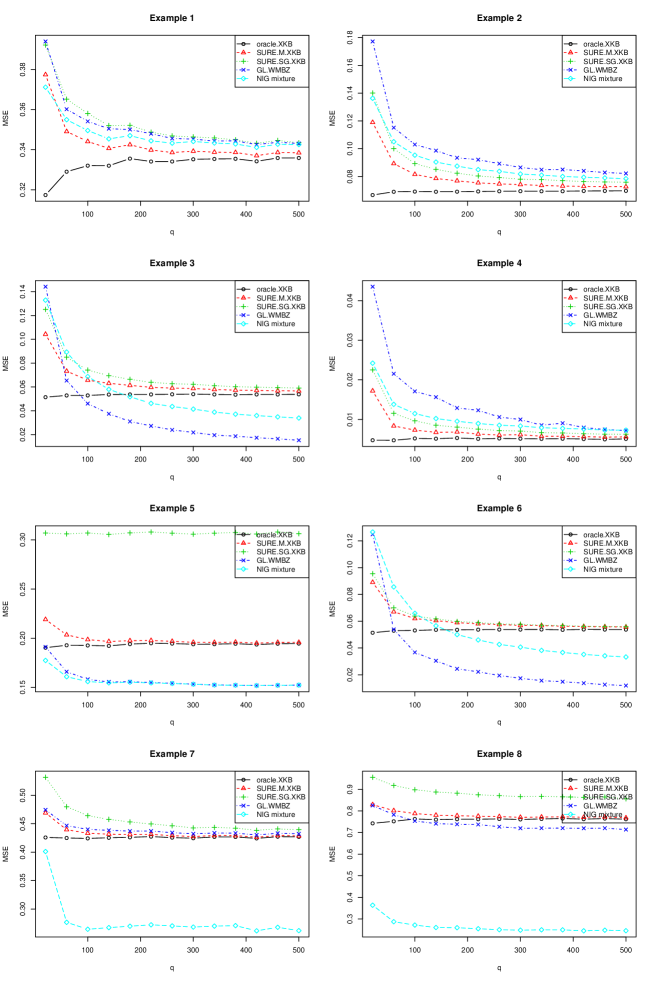
Figure 1: ${\widehat{MSE}}(\bm{\widehat{\mu}},\bm{\mu})$ vs. dimension $q$ of normal vector for Examples 1-8 of Section 4.1. The dimension sizes are $q=20,60,\ldots,500$ and results are based on $1000$ replications at each $q$.

Table 1: Averages of ${\widehat{MSE}}(\bm{\widehat{\mu}},\bm{\mu})$ over all $q=20,60,\ldots,500$ in model (2) for Examples 1-8 of Section 4.1. For a given $q$, ${\widehat{MSE}}(\bm{\widehat{\mu}},\bm{\mu})$ is an average over 1000 replications.

Different				Example
estimates	1	2	3	4	5	6	7	8
Sample Statistics	0.5504	0.5496	0.5506	0.1248	0.3008	0.5502	0.5506	0.8976
EBMLE.XKB	0.3410	0.0762	0.0833	0.0071	0.2524	0.0814	0.4311	0.8448
EBMOM.XKB	0.3412	0.0832	0.0906	0.0086	0.2467	0.0822	0.4313	0.8423
JS.XKB	0.3675	0.0837	0.0885	0.0075	0.2616	0.085	0.4523	0.8563
Oracle.XKB	0.3328	0.0691	0.0535	0.0051	0.1936	0.0535	0.4258	0.7602
SURE.G.XKB	0.3424	0.0792	0.0645	0.0072	0.2365	0.0613	0.4327	0.8393
SURE.M.XKB	0.3433	0.0795	0.0639	0.0072	0.1988	0.0608	0.4334	0.7811
SURE.SG.XKB	0.3526	0.086	0.0699	0.0088	0.3068	0.0621	0.4561	0.8824
SURE.SM.XKB	0.3557	0.0877	0.0698	0.0091	0.1877	0.0628	0.4569	0.6829
GL.WMBZ	0.3512	0.098	0.0373	0.0141	0.1578	0.0306	0.4387	0.7401
GL.SURE.WMBZ	0.3534	0.0974	0.0473	0.0127	0.1578	0.0368	0.4415	0.7249
DGL.WMBZ	0.3714	0.1155	0.1044	0.0158	0.2496	0.0937	0.4523	0.8525
$N\Gamma^{-1}$ mixture	0.3471	0.0894	0.0548	0.0102	0.1560	0.0532	0.2787	0.2639

4.2 Comparing Different Shrinkage Estimators when $\bm{D}$ is Unknown

Tables LABEL:tab:T21 and LABEL:tab:T22 compare the different estimates discussed in Xie et al. (2012), Weinstein et al. (2018) and Jing et al. (2016). The estimate referred to as SURE.M.Double can be found in (11)-(12) of Jing et al. (2016). Although Jing et al. (2016) discussed a few different double shrinkage algorithms, we have found the performance of those algorithms to be very similar to each other, and therefore report results only for the algorithm in expression (16) of Jing et al. (2016), which we refer to as SURE.M.Double. As Xie et al. (2012) and Weinstein et al. (2018) assumed that $\sigma_{1}^{2},\ldots,\sigma_{q}^{2}$ were known, we do as they suggested and replace $\sigma_{j}^{2}$ by $S_{\cdot j}^{2}$ when implementing their algorithms.

We simulated data from model (1) for different choices of $f_{\mu,\sigma^{2}}$. In all the examples of this section $\epsilon\sim N(0,1)$. For each $(\mu_{j},\sigma_{j}^{2})$ pair there are $n=4$ replications. We only observe $X_{ij}$, for $i=1,\ldots,n$, $j=1,\ldots,q$, and not $\sigma_{1}^{2},\ldots,\sigma_{q}^{2}$. We repeat the experiment 1000 times for each $q$, and ${\widehat{MSE}}(\bm{\widehat{\mu}},\bm{\mu})$ and ${\widehat{MSE}}(\bm{\widehat{D}},\bm{D})$ were determined. Tables LABEL:tab:T21 and LABEL:tab:T22 provide estimated risks averaged over all $q$, and Figure 2 shows how our estimate compares with the two SURE estimates discussed in Xie et al. (2012) and with the group-linear algorithms discussed in Weinstein et al. (2018). Figure 3 shows how our estimate of estimating $\bm{D}$ compares with the SURE.M.Double discussed in Jing et al. (2016).

Example 9.

The density $f_{\mu,\sigma^{2}}$ is such that $\mu$ and $\sigma^{2}$ are independent with $\mu\sim N(0,3)$ and $\sigma^{2}\sim IG(5,2)$. Figure 2 shows that our estimate outperforms the other three when estimating $\mu_{j}$. Table LABEL:tab:T21 shows that $N\Gamma^{-1}$ performs similarly to the double shrinkage algorithms discussed in Jing et al. (2016). As the latter algorithms and $N\Gamma^{-1}$ are based on the normal-inverse gamma distribution, and the $(\mu_{j},\sigma_{j}^{2})$ distribution in this case is normal-inverse gamma, it is not surprising that these estimates outperform the others here. Table LABEL:tab:T22 and Figure 3 show that the SURE.M.Double estimate slightly outperforms $N\Gamma^{-1}$ in estimating $\bm{D}$.

Example 10.

The density $f_{\mu,\sigma^{2}}$ is such that $\mu$ and $\sigma^{2}$ are independent with $\mu\sim N(0,3)$ and $\sigma^{2}\sim G(9,3)$. This case is similar to Example 7, and likewise the results are similar.

Example 11.

Here $(\mu,\sigma^{2})\sim 0.95N{\Gamma}^{-1}(2,2,5,2)+0.05N{\Gamma}^{-1}(10,4,3,3)$, the same mixture distribution considered in Example 8. This is a case where $\mu$ and $\sigma^{2}$ are dependent and their distribution is bimodal. Our algorithm outperforms all other estimates in terms of both $\bm{\mu}$ and $\bm{D}$ estimation, as seen in Figures 2-3 and Tables LABEL:tab:T21-LABEL:tab:T22.

Example 12.

In this case $\mu$ and $\sigma^{2}$ are independent with $\mu\sim 0.5U(1,2)+0.5U(4,5)$ and $\frac{\sigma^{2}}{n}\sim U(0.1,1)$. This is a case where $\mu$ and $\sigma^{2}$ are independent and have a bimodal distribution. As in Example 11, the $N\Gamma^{-1}$ estimate outperforms all other estimates with respect to estimating $\mu$. However, presumably because the distribution of $\sigma^{2}$ is unimodal, SURE estimates do better in terms of estimating $\sigma^{2}$.

Example 13.

The distribution of $(\mu,\sigma^{2})$ is such that $\mu\sim N(3,1^{2})$ and $\sigma^{2}|\mu\sim U(\textrm{max}(\mu-1,0.1),\textrm{max}(\mu+1,1))$. Here, $\mu$ and $\sigma^{2}$ are dependent, which is a case where SURE estimates do not perform well. The $N\Gamma^{-1}$ estimate outperforms the other estimates in terms of ${\widehat{MSE}}(\bm{\widehat{\mu}},\bm{\mu})$ and in terms of ${\widehat{MSE}}(\bm{\widehat{D}},\bm{D})$ for larger $q$.

Example 14.

The distribution of $(\mu,\sigma^{2})$ is such that $\mu\sim N(3,1^{2})$ and $\sigma^{2}|\mu\sim\textrm{max}(N(\frac{|\mu|}{3},$ ${(\frac{|\mu|}{3}+1)}^{2}),0.1)$. Again, since $\mu$ and $\sigma^{2}$ are dependent, the SURE estimates do not perform well. The group-linear algorithms lose efficiency as $\sigma_{j}^{2}$ is replaced by $S_{\cdot j}^{2}$, and the $N\Gamma^{-1}$ estimate outperforms all other estimates in terms of both ${\widehat{MSE}}(\bm{\widehat{\mu}},\bm{\mu})$ and ${\widehat{MSE}}(\bm{\widehat{D}},\bm{D})$.

Table 2: Averages of ${\widehat{MSE}}(\bm{\widehat{\mu}},\bm{\mu})$ over all $q=20,60,\ldots,500$ in model (1) for Examples 9-14 of Section 4.2. For a given $q$, ${\widehat{MSE}}(\bm{\widehat{\mu}},\bm{\mu})$ is an average over 1000 replications.

Different			Example
estimates	9	10	11	12	13	14
Sample Statistics	0.1247	0.7484	0.1376	0.5520	0.7525	0.3570
EBMLE.XKB	0.1217	0.6369	0.1795	0.4681	0.4925	0.2432
EBMOM.XKB	0.1217	0.6381	0.1710	0.4690	0.4881	0.2430
JS.XKB	0.1222	0.6637	0.1328	0.5023	0.5997	0.3416
Oracle.XKB	0.1214	0.6350	0.1362	0.4670	0.4491	0.2342
SURE.G.XKB	0.1223	0.6479	0.1373	0.4765	0.4704	0.2428
SURE.M.XKB	0.1224	0.6483	0.1371	0.4769	0.4513	0.2384
SURE.SG.XKB	0.1249	0.6927	0.1343	0.5215	0.5461	0.2662
SURE.SM.XKB	0.1252	0.6954	0.1343	0.5228	0.5289	0.2638
GL.WMBZ	0.1216	0.6644	0.1317	0.4882	0.4958	0.2544
GL.SURE.WMBZ	0.1220	0.6720	0.1310	0.4965	0.5020	0.2589
DGL.WMBZ	0.1200	0.6045	0.1312	0.4538	0.4430	0.2679
SURE.M.Double	0.1199	0.5995	0.1319	0.4493	0.4340	0.2649
$N\Gamma^{-1}$ mixture	0.1198	0.5995	0.0911	0.2849	0.4176	0.2333

Table 3: Averages of ${\widehat{MSE}}(\bm{\widehat{D}},\bm{D})$ over all $q=20,60,\ldots,500$ in model (1) for Examples 9-14 of Section 4.2. For a given $q$, ${\widehat{MSE}}(\bm{\widehat{D}},\bm{D})$ is an average over 1000 replications.

Different			Example
estimates	9	10	11	12	13	14
Sample Statistics	0.2206	6.6980	0.3836	3.9425	1.1918	2.9284
SURE.M.Double	0.0626	0.9160	0.1548	0.8692	0.2873	1.3108
$N\Gamma^{-1}$	0.0689	1.0065	0.1283	0.9630	0.3072	1.0025

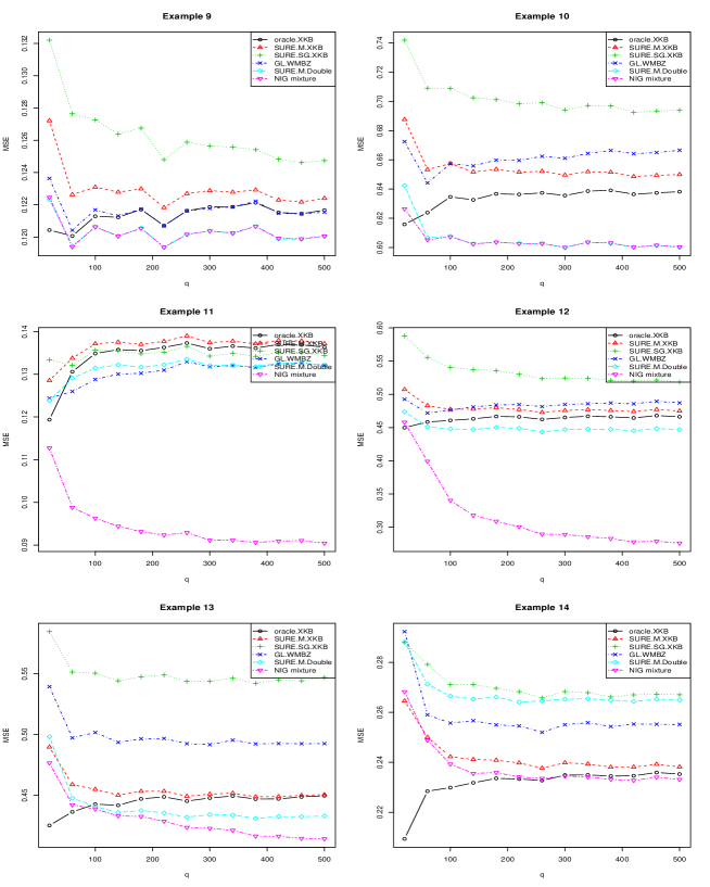
Figure 2: ${\widehat{MSE}}(\bm{\widehat{\mu}},\bm{\mu})$ vs. dimension $q$ of normal vector for Example 9-14 of Section 4.2. The dimension sizes are $q=20,60,\ldots,500$ and results are based on $1000$ replications at each $q$.

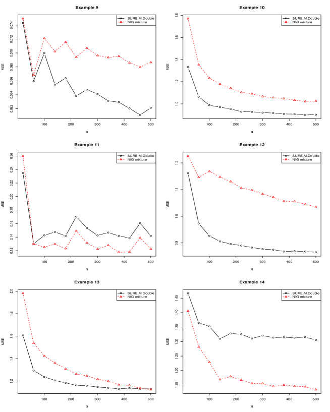
Figure 3: ${\widehat{MSE}}(\bm{\widehat{D}},\bm{D})$ vs. dimension $q$ of normal vector for Examples 9-14 of Section 4.2. The dimension sizes are $q=20,60,\ldots,500$ and results are based on $1000$ replications at each $q$.

We experimented with several choices for $\gamma$, the DPMM concentration parameter. In Example 11 we took $\gamma$ to be 0.1, 10, 50, 100 with $k=10$. Since the true distribution is bimodal, ideally the DP process should have only two active components. Table LABEL:tab:T5 shows changing the value of $\gamma$ has very little effect on the mean squared error of either $\hat{\bm{\mu}}$ or $\hat{\bm{D}}$. On the other hand Figures 4 and 5 show that a lower value of $\gamma$ does a better job of selecting the number of clusters. The higher values of $\gamma$ over-select the number of active components but at least two of the active components have very similar $N\Gamma^{-1}$ parameters, implying that the shrinkage direction and factor for each $\mu_{j}$ changes little. The result is almost no change in mean squared error as long as $k<q$. For Figure 4 and 5, we need to estimate $\bm{\pi}$, which we are calculating by averaging over all MCMC iteration. Due to the non-identifiability arising from permutations of the labels in the mixture representation, we sort $\bm{\pi}$ in every MCMC iteration, and then average results estimate the $2^{nd}$ and $3^{rd}$ highest probabilities. Presumably sorting $\bm{\pi}$ in every iteration will mitigate the label switching problem as in the true $f_{\mu,\sigma^{2}}$ two mixing probabilities are very different from each other.

Table 4: Averages of measures over all $q=20,60,\ldots,500$ in model (1) for Example 11 of Section 4.2. For a given $q$, each measure is an average over 100 replications.

Different
measures	$\gamma=0.1$	$\gamma=10$	$\gamma=50$	$\gamma=100$
${\widehat{MSE}}(\bm{\widehat{\mu}},\bm{\mu})$	0.0937	0.0954	0.0965	0.0966
${\widehat{MSE}}(\bm{\widehat{D}},\bm{D})$	0.1863	0.2063	0.2081	0.2059

Figure 4: Box plot of estimated $\pi_{(8)}$, the $3^{rd}$ highest probability for $q=20,60,\ldots,500$ in model (1) for Example 11 of Section 4.2. For a given $q$, each boxplot is drawn using 100 simulations.

Figure 5: Box plot of estimated $\pi_{(9)}$, the $2^{nd}$ highest probability for $q=20,60,\ldots,500$ in model (1) for Example 11 of Section 4.2. The true value of this parameter is 0.05. For a given $q$, each boxplot is drawn using 100 simulations.

5 Real data example when ${\bf D}$ is known

In this section, we consider a baseball data example as a test case for our $N\Gamma^{-1}$ mixture estimate. This data set has been used in the articles of Brown (2008), Xie et al. (2012), Jing et al. (2016), and Weinstein et al. (2018). The data consist of the entire season batting records for all major league baseball players in the 2005 season. The goal is to estimate batting averages of individual players in the second half of the season by observing only the first half averages. Following the other articles, only players with at least 11 at-bats in the first half of the season were considered in the estimation process, and only players with at least 11 at-bats in each of the two halves of the season were considered in the validation process.

Let $H_{ij}$ denote the number of hits and $N_{ij}$ the number of at-bats for player $j$ in period $i$. The subscript $i$ indicates either the first or second half of the season. The quantity $p_{j}$ denotes the probability of a hit for player $j$. Then we assume that

$$H_{ij}\sim\textrm{Bin}(N_{ij},p_{j}),\quad\textrm{for}\quad i=1,2,\quad j=1,\ldots,q,$$

where $\textrm{Bin}(n,p)$ denotes a binomial distribution with number of trials $n$ and probability of success $p$. Without doing any variance-stabilizing transformation, Jing et al. (2016) worked with the sample proportion $X_{1j}=H_{1j}/N_{1j}$ and the estimated variance, $S_{1j}^{2}=(X_{1j}(1-X_{1j}))/N_{1j}$, of $X_{1j}$. However, this contradicts their initial assumption that $X_{1j}$ and $S_{1j}^{2}$ are independently distributed. Also, without the transformation there is no reason to believe that $X_{1j}$ is normally distributed and $S_{1j}^{2}$ follows a chi-square distribution. So, we will follow the transformation of Brown (2008), which was also used in Xie et al. (2012) and Weinstein et al. (2018), and define

$$X_{ij}=\textrm{arcsin}\sqrt{\frac{H_{ij}+0.25}{N_{ij}+0.5}},$$

resulting in

$$X_{ij}\dot{\sim}N(\mu_{j},\sigma_{ij}^{2}),\quad\mu_{j}=\textrm{arcsin}\left(\sqrt{p}_{j}\right),\quad\sigma_{ij}^{2}={(4N_{ij})}^{-1}.$$

The measure of error that was used in all these papers, denoted TSE, is used to compare different estimates:

$$TSE(\bm{\hat{\mu}})=\frac{\sum_{j}{(X_{2j}-\hat{\mu}_{j})}^{2}-\sum_{j}{(4N_{2j})}^{-1}}{\sum_{j}{(X_{2j}-X_{1j})}^{2}-\sum_{j}{(4N_{2j})}^{-1}}.$$

The transformed data are consistent with model (2) as all $\sigma_{j}^{2}$ are known. The MCMC algorithm described in Section 3 is modified here by simply removing the step of updating $\sigma_{j}^{2}$. Table LABEL:tab:T3 is the table from Weinstein et al. (2018) with our estimate added in the bottom row.

Table 5: Average Prediction error for transformed batting averages. $TSE(\bm{\hat{\mu}})$ was computed for the entire data set, and separately for pitchers and non-pitchers.

Different		Data sets
estimates	All	Pitchers	Non-pitchers
Naive	1	1	1
Grand mean	0.852	0.127	0.378
Nonparametric EB	0.508	0.212	0.372
Binomial mixture	0.588	0.156	0.314
Weighted Least Squares	1.07	0.127	0.468
Weighted nonparametric MLE	0.306	0.173	0.326
Weighted Least Squares (AB)	0.537	0.087	0.29
Weighted nonparametric MLE (AB)	0.301	0.141	0.261
JS.XKB	0.535	0.165	0.348
SURE.M.XKB	0.421	0.123	0.289
SURE.SG.XKB	0.408	0.091	0.261
GL.WMBZ	0.302	0.178	0.325
DGL.WMBZ	0.288	0.168	0.349
$N\Gamma^{-1}$ mixture	0.361	0.161	0.292

The naive estimator simply uses $X_{1j}$ to predict $X_{2j}$ and has TSE equal to 1. The grand mean uses the average of all $X_{1j}$ to predict any $X_{2j}$. The nonparametric EB estimate of Brown and Greenshtein (2009), the binomial mixture of Muralidharan (2010), the weighted least squares estimator, the weighted least squares estimator (AB) (with number of at-bats as covariate), the weighted nonparametric MLE and the weighted nonparametric MLE (AB) (with number of at-bats as covariate) of Jiang et al. (2009) are also included in Table LABEL:tab:T3.

Weinstein et al. (2018) presented an analysis under permutations, where each permutation is the order in which successful hits appear throughout the entire season. For each player they draw the number of hits in $N_{1j}$ at-bats from a hypergeometric distribution, $HG(N_{1j}+N_{2j},H_{1j}+H_{2j},N_{1j})$. We compare our estimate with several other estimates with respect to $1000$ different permutations of the baseball data and average TSE.

As discussed in Weinstein et al. (2018), group-linear algorithms tend to perform well compared to SURE estimates as $\mu_{j}$ and $\sigma_{1j}^{2}$ are not independent, owing to the fact that players with higher batting averages tend to play more. Also, non-pitchers tend to have higher batting averages than pitchers, so it is possible that the underlying density of $\mu$ is bimodal. This may be the reason that empirical Bayes estimators that assume a normal-normal model tend to perform poorly. group-linear estimates outperform the other estimates because they can accommodate these features exhibited by the baseball data. SURE estimates work well when we analyze the pitchers and non-pitchers separately. Table LABEL:tab:T3 shows that, in the combined data, the $N\Gamma^{-1}$ estimate does not perform as well as group-linear algorithms, but it performs better than SURE estimates. However, when the pitchers and non-pitchers are considered separately, $N\Gamma^{-1}$ performs better than the group-linear algorithms. In both the original data and the permuted data, $N\Gamma^{-1}$ performs better than the group-linear algorithms for both pitchers and non-pitchers. When pitchers and non-pitchers are combined, group-linear estimates outperform all other estimates in both the original and permuted data. This is reasonable as the association between $\mu$ and $\sigma^{2}$ is weaker when the data are separated into smaller groups, and group-linear algorithms work well in the presence of strong association. In contrast, the $N\Gamma^{-1}$ estimate works reasonably well $\mu$ and $\sigma^{2}$ are either strongly or weakly dependent.

Table 6: Average Prediction error for 1000 permutations of transformed batting averages data. Average $TSE(\bm{\hat{\mu}})$ was computed for the entire data set, and separately for pitchers and non-pitchers.

Different		Data sets
estimates	All	Pitchers	Non-pitchers
Grand mean	0.9222	0.3127	0.2951
James-Stein	0.5465	0.2490	0.2304
SURE.M.XKB	0.4852	0.2227	0.2602
SURE.SG.XKB	0.4693	0.1759	0.2148
GL.WMBZ(bins = $q^{1/3}$)	0.2798	0.2438	0.1731
GL.SURE.WMBZ	0.3032	0.2838	0.1949
DGL.WMBZ	0.4751	0.2193	0.2250
$N\Gamma^{-1}$ mixture	0.3535	0.2377	0.1698

6 Real data example when ${\bf D}$ is unknown

In this section, we will apply the $N\Gamma^{-1}$ estimate and other estimators to the prostate data from the book of Efron (2012). The data can be downloaded from the book website https://statweb.stanford.edu/~ckirby/brad/LSI/datasets-and-programs/data/. The pros- tate data consist of genetic expression levels for $q=6033$ genes obtained from 102 men, 50 normal control and 52 prostate cancer patients. We only use the control data, which means that we have a $50\times 6033$ matrix. Here $X_{ij}$ denotes the expression level for gene $j$ of patient $i$, $i=1,\ldots,50$, $j=1,\ldots,6033$. Since $50$ is a relatively large number, we will assume that the control group constitutes the population of interest, in which case

$$\mu_{j}=\frac{1}{50}\sum_{i=1}^{50}X_{ij}\quad\textrm{and}\quad\sigma_{j}^{2}=\frac{1}{50}\sum_{i=1}^{50}{(X_{ij}-\mu_{j})}^{2},\quad j=1,\ldots,6033.$$

As a test of the various estimates, we randomly select three subjects from the control group and use their data to estimate $\mu_{j}$ and $\sigma_{j}^{2}$.

To better understand the nature of the data we provide the scatterplots in Figures 6-7. We also compared our estimate with the sample means and variances from three columns.

Figure 6: Scatterplots for prostate data. The upper left plot is $S_{\cdot j}^{2}$ vs. $\bar{X}_{\cdot j}$ for columns $6$, $30$ and $31$ of the data matrix, the upper right plot is $\sigma_{j}^{2}$ vs. $\mu_{j}$ and the lower left plot is ${\hat{\sigma}_{j,DPMM}}^{2}$ vs. ${\hat{\mu}_{j}}^{DPMM}$ based on columns $6$, $30$ and $31$.

Figure 7: Scatterplots for prostate data based 3 columns $6$, $30$ and $31$ of the data matrix. The upper left plot is $\bar{X}_{\cdot j}$ vs. $\mu_{j}$, the upper right plot is ${\hat{\mu}_{j}}^{DPMM}$ vs. $\mu_{j}$ based on columns $6$, $30$ and $31$. The lower left plot is $\bar{S}_{\cdot j}^{2}$ vs. $\sigma_{j}^{2}$, the lower right plot is ${\hat{\sigma}_{j,DPMM}}^{2}$ vs. $\sigma_{j}^{2}$ based on columns $6$, $30$ and $31$.

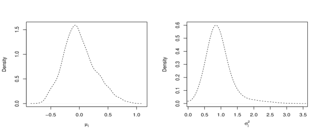
Figure 8: Marginal kernel density estimates computed from $\mu_{j}$ and $\sigma_{j}^{2}$ based on all 50 columns of the data matrix.

To compare different estimates we randomly chose 500 rows and 3 columns, computed estimates of means and variances using the various estimates, and replicated this process 100 times. Average squared error for each estimate was computed as in our simulation study. Table LABEL:tab:T10 shows that, except for the SURE-based Double shrinkage estimators, all estimates were outperformed by $N\Gamma^{-1}$. Figure 8 shows that the densities of $\mu_{j}$ and $\sigma_{j}^{2}$ are well-approximated by normal and inverse gamma densities, respectively. When we force the mixture of normal-inverse gammas to select only one component, then this estimate performs comparably to SURE.M.Double for estimating both $\bm{\mu}$ and $\bm{D}$. For the other algorithms, replacing the unknown $\sigma_{j}^{2}$ with $S_{\cdot j}^{2}$ results in a loss in accuracy of those estimates.

Table 7: Estimated average squared loss for $\bm{\mu}$ and $\bm{D}$ for different estimates from prostate-control data. Each table value is an average over $100$ replications. Each replication consists of 500 randomly chosen rows and $3$ randomly chosen columns from the original $6033\times 50$ data matrix.

Different	Different measures
estimates	Error in estimating $\mu_{j}$	Error in estimating $\sigma_{j}^{2}$
Sample Statistics	0.2919	1.1695
EBMLE.XKB	0.1486	-
EBMOM.XKB	0.1446	-
JS.XKB	0.2787	-
Oracle.XKB	0.1108	-
SURE.G.XKB	0.1071	-
SURE.M.XKB	0.1175	-
SURE.SG.XKB	0.1445	-
SURE.SM.XKB	0.1682	-
GL.WMBZ	0.1694	-
GL.SURE.WMBZ	0.1802	-
DGL.WMBZ	0.0690	-
SURE.M.Double	0.0644	0.1458
$N\Gamma^{-1}$ mixture	0.1081	0.2284
$N\Gamma^{-1}$ one component	0.0683	0.1653

7 Summary

Since Stein’s work (Stein (1956)), there has been much progress in using shrinkage estimators of the mean of a high-dimensional normal vector. However, all of the previous work shrinks the sample means in the same direction. We have developed a very general algorithm which does not rely on the belief that all $\mu_{j}$ are of the same magnitude. Our estimate works by clustering sample means into different groups, and then shrinking an individual mean towards its corresponding group mean. Our algorithm outperforms SURE estimates when $\mu_{j}$ and $\sigma_{j}^{2}$ are dependent, and outperforms group-linear algorithms when $\mu_{j}$ and $\sigma_{j}^{2}$ are independent. When $\mu_{j}$ has a multimodal distribution or when $\sigma_{j}^{2}$ is unknown, our estimate based on mixtures of normal-inverse gamma distributions performed better than all the other estimates with which it was compared. Also, our approach allows us to estimate the joint density of $(\mu_{j},\sigma_{j}^{2})$, a problem which seems not to have been previously addressed. All code for our methodology is available online at https://github.com/shyamalendusinha/mean_estimation.

References

- Baranchik [1970] Alvin J Baranchik. A family of minimax estimators of the mean of a multivariate normal distribution. The Annals of Mathematical Statistics, pages 642–645, 1970.
- Berger [1976] James O Berger. Admissible minimax estimation of a multivariate normal mean with arbitrary quadratic loss. The Annals of Statistics, pages 223–226, 1976.
- Berger and Strawderman [1996] James O Berger and William E Strawderman. Choice of hierarchical priors: admissibility in estimation of normal means. The Annals of Statistics, pages 931–951, 1996.
- Brown [1971] Lawrence D Brown. Admissible estimators, recurrent diffusions, and insoluble boundary value problems. The Annals of Mathematical Statistics, 42(3):855–903, 1971.
- Brown [2008] Lawrence D Brown. In-season prediction of batting averages: A field test of empirical bayes and bayes methodologies. The Annals of Applied Statistics, pages 113–152, 2008.
- Brown and Greenshtein [2009] Lawrence D Brown and Eitan Greenshtein. Nonparametric empirical bayes and compound decision approaches to estimation of a high-dimensional vector of normal means. The Annals of Statistics, pages 1685–1704, 2009.
- Efron [2012] Bradley Efron. Large-scale inference: empirical Bayes methods for estimation, testing, and prediction, volume 1. Cambridge University Press, 2012.
- Efron and Morris [1973] Bradley Efron and Carl Morris. Stein’s estimation rule and its competitors – an empirical bayes approach. Journal of the American Statistical Association, 68(341):117–130, 1973.
- Escobar and West [1995] Michael D Escobar and Mike West. Bayesian density estimation and inference using mixtures. Journal of the American Statistical Association, 90(430):577–588, 1995.
- Ferguson [1983] Thomas S Ferguson. Bayesian density estimation by mixtures of normal distributions. Recent advances in statistics, 24(1983):287–302, 1983.
- Ishwaran and James [2001] Hemant Ishwaran and Lancelot F James. Gibbs sampling methods for stick-breaking priors. Journal of the American Statistical Association, 96(453):161–173, 2001.
- James and Stein [1961] William James and Charles Stein. Estimation with quadratic loss. In Proceedings of the fourth Berkeley symposium on mathematical statistics and probability, pages 361–379, 1961.
- Jiang et al. [2009] Wenhua Jiang, Cun-Hui Zhang, et al. General maximum likelihood empirical bayes estimation of normal means. The Annals of Statistics, 37(4):1647–1684, 2009.
- Jing et al. [2016] Bing-Yi Jing, Zhouping Li, Guangming Pan, and Wang Zhou. On sure-type double shrinkage estimation. Journal of the American Statistical Association, 111(516):1696–1704, 2016.
- Lehmann and Casella [2006] Erich L Lehmann and George Casella. Theory of point estimation. Springer Science & Business Media, 2006.
- Lindsay et al. [1983] Bruce G Lindsay et al. The geometry of mixture likelihoods: a general theory. The Annals of Statistics, 11(1):86–94, 1983.
- Muralidharan [2010] Omkar Muralidharan. An empirical bayes mixture method for effect size and false discovery rate estimation. The Annals of Applied Statistics, pages 422–438, 2010.
- Neyman and Scott [1948] Jerzy Neyman and Elizabeth L Scott. Consistent estimates based on partially consistent observations. Econometrica: Journal of the Econometric Society, pages 1–32, 1948.
- Rousseau and Mengersen [2011] Judith Rousseau and Kerrie Mengersen. Asymptotic behaviour of the posterior distribution in overfitted mixture models. Journal of the Royal Statistical Society: Series B (Statistical Methodology), 73(5):689–710, 2011.
- Sethuraman [1994] Jayaram Sethuraman. A constructive definition of dirichlet priors. Statistica Sinica, pages 639–650, 1994.
- Silverman [1986] Bernard W Silverman. Density estimation for statistics and data analysis, volume 26. CRC press, 1986.
- Stein [1956] Charles Stein. Inadmissibility of the usual estimator for the mean of a multivariate normal distribution. Technical report, STANFORD UNIVERSITY STANFORD United States, 1956.
- Tan et al. [2015] Zhiqiang Tan et al. Improved minimax estimation of a multivariate normal mean under heteroscedasticity. Bernoulli, 21(1):574–603, 2015.
- Weinstein et al. [2018] Asaf Weinstein, Zhuang Ma, Lawrence D Brown, and Cun-Hui Zhang. Group-linear empirical Bayes estimates for a heteroscedastic normal mean. Journal of the American Statistical Association, pages 1–13, 2018.
- Xie et al. [2012] Xianchao Xie, SC Kou, and Lawrence D Brown. Sure estimates for a heteroscedastic hierarchical model. Journal of the American Statistical Association, 107(500):1465–1479, 2012.
- Zhang and Bhattacharya [2017] Xianyang Zhang and Anirban Bhattacharya. Empirical bayes, sure and sparse normal mean models. arXiv preprint arXiv:1702.05195, 2017.