The binary black hole explorer: on-the-fly visualizations of precessing binary black holes

Abstract

Binary black hole mergers are of great interest to the astrophysics community, not least because of their promise to test general relativity in the highly dynamic, strong field regime. Detections of gravitational waves from these sources by LIGO and Virgo have garnered widespread media and public attention. Among these sources, precessing systems (with misaligned black-hole spin/orbital angular momentum) are of particular interest because of the rich dynamics they offer. However, these systems are, in turn, more complex compared to nonprecessing systems, making them harder to model or develop intuition about. Visualizations of numerical simulations of precessing systems provide a means to understand and gain insights about these systems. However, since these simulations are very expensive, they can only be performed at a small number of points in parameter space. We present binaryBHexp, a tool that makes use of surrogate models of numerical simulations to generate on-the-fly interactive visualizations of precessing binary black holes. These visualizations can be generated in a few seconds, and at any point in the 7-dimensional parameter space of the underlying surrogate models. With illustrative examples, we demonstrate how this tool can be used to learn about precessing binary black hole systems.

1 Introduction

The merger of two black holes (BHs) is one of the most violent events in the Universe. In the span of a few seconds, the incredible amount of energy $\mathchar 21016\relax 10^{60}$MeV [1] is liberated in gravitational waves (GWs). These “ripples in spacetime” travel across the Universe at the speed of light to our detectors, providing us unique insights into these spectacular astrophysical events.

The first direct detection [1] of GWs from a BH merger was achieved in 2015 by the LIGO [2] twin detectors. This is one of the greatest achievements in modern science, crowning decades of theoretical and experimental efforts in gravitational physics. The detection of GWs not only earned the 2017 Nobel Prize in physics [3], but also sparked an unprecedented interest in science among the general public. For a few days, BHs were on the front pages of most newspapers in the world!

Despite the immense technical difficulties in detecting them, astrophysical BHs are remarkably simple objects, characterized only by their mass and spin. From far away they can be thought of as the analogs of Newtonian point masses in Einstein’s general relativity (GR). Near a BH, departures from Newtonian gravity such as the event horizon, gravitational lensing, gravitational time dilation, frame dragging, etc, become apparent.

When in a binary system, the departure is even more drastic. First, there are no stable binary orbits in GR: emission of GWs takes away energy, angular momentum, and linear momentum from the system, causing the binary’s orbit to shrink. Second, in Newtonian gravity, a point-mass binary orbit that starts in the equatorial plane remains in the equatorial plane. In GR, on the other hand, if the BH spins are misaligned with respect to the orbital angular momentum, relativistic spin-spin and spin-orbit couplings cause the system to precess [4, 5, 6, 7]. Much like a top whose spin axis is misaligned with the orbital angular momentum, the spins and the orbital angular momentum oscillate about the direction of the total angular momentum. This precession is imprinted on the observed gravitational waves as characteristic modulations of amplitude and frequency.

The evolution of a binary BH system can be divided into three stages: inspiral, merger, and ringdown. During the inspiral, the BHs gradually approach each other due to loss of energy and angular momentum to GWs. As they get closer, they eventually coalesce and merge. After the merger, one is left with a single, but highly distorted, BH. In the final stage, called ringdown, all these perturbations (“hairs”) are radiated away and the remnant settles down to its final steady state. The remnant BH is characterized entirely by it mass, spin, and recoil velocity (or “kick”). These properties are associated with the asymptotic conservation laws of energy, angular momentum, and linear momentum, respectively.

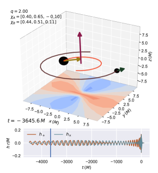
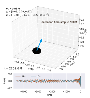
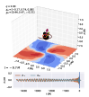
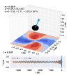
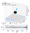
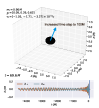
Figure 1: Snapshots during the inspiral (top-left), post-ringdown (top-right), and intermediate (bottom) stages of a precessing binary BH evolution. Each BH horizon is represented by an oblate spheroid. The arrows on the BHs indicate the spin vectors; the larger the spin the longer the arrow. The arrow centered at the origin indicates the orbital angular momentum. On the bottom plane, we show the plus polarization of GWs, as seen by an observer at each point. Red (blue) colors indicate positive (negative) values. Notice the quadrupolar nature of the emitted waves. The subplots at the bottom of each panel show GW plus and cross polarizations, as seen by a far-away observer viewing from the camera viewing angle. The time to the peak of the waveform amplitude is indicated in the figure text as well as the slider in the bottom subplots. This animation is available at vijayvarma392.github.io/binaryBHexp/#prec_bbh.

Modeling GWs emitted during all three stages is crucial to interpreting observations from detectors like LIGO [2] and Virgo [8]. The merger phase, in particular, can only be captured accurately with expensive numerical-relativity (NR) simulations (see e.g. Ref. [9] for a review). Obtaining a single merger waveform prediction might take months of computational time on powerful supercomputers. Visualizations [10] of these simulations have been instrumental in disseminating GW discoveries for outreach and educational purposes. To some extent, experts in the field also rely on visual products to develop intuition and illuminate future directions for research. In particular, visualizations of precessing binary BHs can give valuable insights into their complex dynamics. Available visualizations directly rely on NR simulations, and are therefore restricted to the small number of configurations which have been simulated. Generating a new visualization at a generic point in parameter space would involve a new, expensive NR simulation.

In this paper, we present the “binary Black Hole explorer” (binaryBHexp): a new tool to generate on-the-fly, yet accurate, interactive visualizations of precessing binary black hole evolutions with arbitrary parameters. We rely on recent NR surrogate models. Trained against several hundreds of numerical simulations, these models have been shown to accurately model both the emitted gravitational waveform [11] and the BH remnant properties [12] of precessing binary BH systems. With our easy-to-install-and-use Python package, one can generate visualizations within a few seconds on a standard, off-the-shelf, laptop computer. Some examples are available at vijayvarma392.github.io/binaryBHexp.

Figure 1 shows snapshots from a visualization generated with binaryBHexp. During the inspiral, both radiation reaction and spin precession are at play. While the separation shrinks because of GW emission, the orientations of the spins, and the orbital angular momentum, all vary in time. The GW emission frequency gradually scales as $f\sim r_{12}^{-3/2}$, and amplitude scales as $h\sim r_{12}^{-1}$, where $r_{12}$ is the binary separation, producing a distinctive “chirp” where both frequency and amplitude sweep up over time. GWs are emitted in two polarizations, $h_{+}$ and $h_{\times}$, as predicted by Einstein’s GR. As explored later, the relative amplitude of the two polarizations crucially depends on orientation of the observer with respect to the binary. Spin precession causes amplitude modulations during the inspiral phase, which are also dependent on the observer orientation. After merger, the component BHs are replaced by a remnant BH, whose properties are determined by conservation laws, as mentioned above. The merger process emits copious gravitational radiation, and corresponds to the peak amplitude of the waveform.

The rest of the paper is organized as follows. Sec. 2 describes methods and approximations employed to generate visualizations such as Fig. 1. In Sec. 3, we demonstrate the power of this tool with several examples aimed at exploring known phenomenology in BH dynamics. Sec. 4 describes code implementation and usage. Finally, we provide concluding remarks in Sec. 5.

2 Methods

2.1 Preliminaries

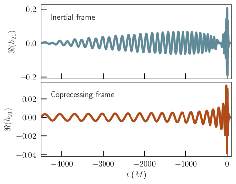
Figure 2: Example of the real part of the $(\ell=2,m=1)$ spin-weighted spherical harmonic mode (see Sec. 2.7) of the GW for a precessing black hole binary, in the inertial (top) and coprecessing (bottom) frames. $t=0$ corresponds to the peak of the waveform amplitude.

We start with some definitions, referring the reader to standard GR and GW textbooks for more details [13, 14, 15, 16, 17, 18]. Throughout this paper, we use geometric units with $G=c=1$.

An isolated astrophysical BH is characterized entirely by its mass $m$ and spin angular momentum $\mathbf{S}=\bm{\chi}m^{2}$. $\bm{\chi}$ is the dimensionless spin, with magnitude $\chi\leq 1$, and $\bm{a}=\bm{\chi}m$ is the Kerr parameter.

A quasicircular precessing binary BH system is characterized by seven intrinsic parameters: mass ratio $q=m_{1}/m_{2}$, and two spin vectors $\bm{\chi}_{1}$, $\bm{\chi}_{2}$. Here, subscript 1 (2) corresponds to the heavier (lighter) of the two BHs. The total mass of the system $M=m_{1}+m_{2}$ can be scaled out. Therefore, throughout this paper, all length and time quantities are in units of $M$. Similarly, all frequency quantities are in units of $1/M$. After the merger takes place, the remnant BH is characterized by its mass $m_{f}$, spin $\bm{\chi}_{f}$ and recoil velocity $\bm{v}_{f}$.

If the BH spins are (anti-)aligned with respect to the orbital angular momentum $\bm{L}$, the emitted GWs have monotonically increasing amplitude and frequency. Instead, if the component spins are misaligned with respect to $\bm{L}$, couplings between the momenta $\bm{L}$, $\bm{S}_{1}$, and $\bm{S}_{2}$ cause them to precess about the direction of the total angular momentum $\bm{J}=\bm{L}+\bm{S}_{1}+\bm{S}_{2}$. GW amplitude and frequency are not monotonic, and their modulations strongly depend on the viewing angle [4]. This complexity can be in part removed by moving into a non-inertial reference frame which tracks the direction of $\bm{L}$ [19, 20, 21]. In this coprecessing frame, the waveform looks nearly as simple as that of a nonprecessing source (cf. bottom panel of Fig. 2), and can be modeled with methods developed to study nonprecessing systems.

2.2 Surrogate models

NR surrogate models provide a fast-but-accurate method to model GW signals. We use a model developed by Blackman et al. [11] named NRSur7dq2 to predict both the waveform and the BH spin dynamics. NRSur7dq2 was trained against 886 NR simulations in the 7-dimensional parameter space of mass ratios $q\leq 2$, and dimensionless spin magnitudes $\chi_{1},\chi_{2}\leq 0.8$. NRSur7dq2 predicts both the emitted GWs and the associated BH spin dynamics. In particular, it models four important quantities that we make use of in this work: (i) the waveform modes $h_{\ell m}$ expanded in spin-weighted spherical harmonics (cf. Sec. 2.7); (ii) the unit quaternions $\hat{Q}(t)$ describing the rotation between the coprecessing frame and a specified inertial frame; (iii) the orbital phase in the coprecessing frame $\phi_{\rm orb}$; and (iv) the precession of component spins $\bm{\chi}_{1}$, $\bm{\chi}_{2}$ over time.

Modeling the BH remnant’s properties is performed with the surrogate surfinBH7dq2 [12], which was also trained on the same set of NR simulations. This model takes in mass ratio $q$ and component spin vectors $\bm{\chi}_{1}$, $\bm{\chi}_{2}$ at a given orbital frequency, and models the remnant mass $m_{f}$, spin vector $\bm{\chi}_{f}$, and kick vector $\bm{v}_{f}$.

2.3 Black-hole shapes

In our visualizations, we represent BH horizons with ellipsoids of revolution. The axis of symmetry is along the instantaneous spin of the BH. The polar (along the axis) and the equatorial (orthogonal to the axis) horizon radii are set to

$$r_{\rm pol}=r_{+}\,,\qquad r_{\rm equi}=\sqrt{r_{+}^{2}+a^{2}}\,,$$ (1)

where $r_{+}=m+\sqrt{m^{2}-a^{2}}$. $r_{\rm pol}$ and $r_{\rm equi}$ correspond to the Kerr-Schild [22, 18] coordinate distances from the BH center to the pole/equator of the horizon. Note that numerical simulations use a different coordinate system, meaning the BH shapes would be different even for an isolated BH. However, this captures the azimuthal symmetry and oblate nature seen in most coordinate systems.

This approximation, however, neglects much of the interesting phenomenology of event horizons (EHs) of BHs in binaries [15, 23, 24]. Event horizons are defined globally, so the locations of EHs cannot be determined without knowing the entire future development of a spacetime. Most NR simulations track the location of apparent horizons (AHs) [15], which can be defined locally. Both EHs and AHs of orbiting BHs are deformed by the tidal field of the other BH. This distortion becomes very strong close to merger, where the shape of the two event horizons do not resemble, even vaguely, that of ellipsoids (see e.g. [25]). Improving our representation of EH shapes requires building surrogate models for the morphology of the EH/AH, which is an interesting avenue for future work.

In addition, we assume the masses of the BHs are constant during the evolution. While the masses in an NR simulation can change due to in-falling energy through GWs, this is a very small effect (4PN (Post Newtonian) higher than leading orbital energy loss [26, 27, 28]) that is safely ignored in current waveform models including NRSur7dq2.

2.4 Component black-hole spin evolution

The two spins $\bm{\chi}_{1},\bm{\chi}_{2}$ are modeled using NRSur7dq2. These are known to agree well with NR simulations and are crucial for the accuracy of that waveform model [11]. Note, however, that the spins modeled by NRSur7dq2 have had an additional smoothing filter applied to remove short-timescale oscillations [11]. This approximation propagates to our visualizations. Similarly to the masses of the BHs, we assume the spin magnitudes are constant during the evolution. In-falling angular momentum in the form of GWs can alter the spin magnitudes, but this is also a very small effect (4PN higher than leading angular-momentum loss [27, 28]) that is ignored by current waveform models including NRSur7dq2.

Spins are represented as arrows centered at the BH centers, that are proportional to the Kerr parameter $\bm{a}$ of each BH. More specifically, the length is set to $10a$, and the direction is along $\hat{\bm{a}}$. The exaggeration of the magnitude is necessary to make the spin vectors clearly visible during the evolution; more on this in the next section.

2.5 Orbital angular momentum

NRSur7dq2 only predicts the unit rotation quaternion $\hat{Q}(t)$ and not the magnitude $L$. The (time dependent) direction of orbital plane is inferred from $\hat{Q}(t)$ and is orthogonal to the z-axis of the coprecessing frame. For the magnitude $L$, we implement the Newtonian expression

$$L=M^{2}\frac{q}{(1+q)^{2}}~{}(M\omega_{\rm orb})^{-1/3},$$ (2)

where $\omega_{\rm orb}$ is the orbital frequency, as derived from the orbital phase in the coprecessing frame modeled by NRSur7dq2,

$$\omega_{\rm orb}=\frac{d\phi_{\rm orb}}{dt}\,.$$ (3)

In our visualizations, the angular momentum is indicated by an arrow at the origin. Its magnitude is rescaled to $12L$. This factor is arbitrary and it is chosen to make the arrow clearly visible.

Note that it is not appropriate to compare an arrow for orbital angular momentum $L\propto M^{2}$ to those representing the Kerr parameters ${a}_{1},{a}_{2}\propto M$ because they have different dimensions. The choice of representing $a$, rather than the $S\propto M^{2}$ was made to allow all arrows to be clearly visible throughout the inspiral for generic locations in the parameter space (i.e. different mass ratios). However, we provide an option to represent $S$ for the spin arrows (cf. Sec. 4), in which case the arrow magnitudes are set to $12S$. This makes the arrow on the smaller BH barely visible in some cases, but allows direct comparison of the spin arrows to the orbital angular momentum arrow. This could be informative for gaining intuition about peculiar spin phenomena like transitional precession [4, 29], spin orbit resonances [30], large nutations [31, 32] and precessional instabilities [33]. This phenomenology is currently beyond the scope of the surrogate we used, but is being actively researched with NR simulations [34, 35] and lies within the realm of future hybridized surrogate models (see e.g. [36]).

2.6 Component black-hole trajectories

The gauge symmetry of GR is broken in an NR simulation, since one necessarily has to specify a set of coordinates to represent the solution on a computer. The BH trajectories extracted from numerical simulations are, therefore, inherently gauge dependent.

In the construction of NRSur7dq2 [11] quantities like $\hat{Q}(t)$ and $\phi_{\rm orb}$ are obtained from the GWs extrapolated to future null infinity, not from numerical simulations’ BH coordinates.

In our visualizations, we reconstruct the trajectories of the BHs using the dynamics predicted by NRSur7dq2 and some PN arguments. In particular, one needs the separation between the BHs as a function of the orbital frequency, $r_{12}(\omega_{\rm orb})$, with the orbital frequency defined as in Eq. (3). The separation $r_{12}(\omega_{\rm orb})$ is modeled using the 3.5PN expressions reported in Eq. (4.3) of Ref. [37], along with the 2PN spin-spin term from Eq. (4.13) of Ref. [5].

Let us write the coprecessing frame coordinates as $(x^{\prime},y^{\prime},z^{\prime})$. The trajectories in the coprecessing frame, where the orbital plane is orthogonal to the $z^{\prime}-$axis, are given by

$$\begin{cases}x^{\prime}_{1}=r_{1}\cos\phi_{\rm orb}\\ y^{\prime}_{1}=r_{1}\sin\phi_{\rm orb}\\ z^{\prime}_{1}=0\end{cases}\begin{cases}x^{\prime}_{2}=-r_{2}\cos\phi_{\rm orb}\\ y^{\prime}_{2}=-r_{2}\sin\phi_{\rm orb}\\ z^{\prime}_{2}=0\end{cases}$$ (4)

where $r_{1}$ ($r_{2}$) indicates the coordinate separation from the origin to the primary (secondary) BH center. We use the Newtonian relations

$$r_{1}=\frac{m_{2}}{M}~{}r_{12},\qquad r_{2}=\frac{m_{1}}{M}~{}r_{12},$$ (5)

to enforce the Newtonian center-of-mass of the binary to be at the origin. This ignores the fact that true center of mass during inspiral and merger oscillates about the origin due to linear momentum carried away in GW. However, this correction would be too small to be noticeable on the scale of our visualizations (see e.g. Fig. 2 of [38]).

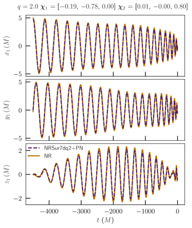
Figure 3: Comparison of the coordinate trajectories of the heavier BH for a precessing binary BH, between NR, and our approximation using NRSur7dq2 and PN. $t=0$ corresponds to the peak of the waveform amplitude. The mass ratio, and spins at $t=-4500M$ are shown at the top of the plot.

Given the trajectories in the coprecessing frame, the trajectories in the inertial frame are obtained by a quaternion transformation with the time-dependent rotation (unit) quaternions $\hat{Q}(t)$ (for a brief introduction to quaternions in this context, see e.g. App. A of [39]). Treating the Euclidean positions as purely imaginary quaternions, the transformation is

$$\bm{x}_{i}=\hat{Q}(t)~{}\bm{x}^{\prime}_{i}~{}\hat{Q}^{-1}(t)\,.$$ (6)

Figure 3 compares the trajectories predicted by our method to the gauge-dependent ones extracted from an NR simulation. Our approximate trajectories turn out to be remarkably close to the NR trajectories. The dominant deviations are due to the PN formulae being in harmonic gauge, whereas the NR simulations use the damped harmonic gauge [40].

2.7 Gravitational waves

NR simulations predict the entire spacetime metric of a binary BH evolution. However, the full metric is usually discarded because most applications (notably GW observations) only require the gravitational waves as seen by an observer far away.

Indeed, splitting the metric into GWs and a non-oscillatory part can only be well defined in the wave zone, which is at distances $r$ much larger than the gravitational wavelength $\lambda$. Let us suppose we are in a spacetime that is approximately Minkowski space, with a metric perturbation $h_{ab}$, in the transverse-tracefree (TT) gauge [41]. We define a spherical polar coordinate system $(t,r,\theta,\phi)$ with the binary center-of-mass at the origin. The $z$ axis ($\theta=0$) of this coordinate system is parallel to $\bm{L}$ at some reference time/frequency. The $x$ axis lies along the line of separation from the lighter BH to the heavier BH at this time/frequency, and the $y$ axis completes the triad.

The spherically outgoing gravitational wave is typically converted into a spin-weight $-2$ complex scalar by contracting $h\equiv h_{ab}\bar{m}^{a}\bar{m}^{b}$, where $m^{a}=(\hat{e}_{\theta}^{a}+i\hat{e}_{\phi}^{a})/\sqrt{2}$ is an element of a complex null dyad [18] along with its conjugate $\bar{m}^{a}$; and where $\hat{e}_{\theta}^{a},\hat{e}_{\phi}^{a}$ are the standard unit vectors in the $\theta$ and $\phi$ directions, respectively. The gravitational-wave strain $h$ is then decomposed as

$$h(t,r,\theta,\phi)=\sum_{\ell=2}^{\infty}\,\sum_{m=-\ell}^{\ell}{}_{-2}Y_{\ell m}(\theta,\,\phi)\,h_{\ell m}(t,r)\,,$$ (7)

where ${}_{-2}Y_{\ell m}$ are the $s\!=\!-2$ spin-weighted spherical harmonics [42]. The functions $h_{\ell m}$ are referred to as the modes of the GWs.

From the structure of the flat-space d’Alembertian operator, we can see that at large distances, $h$ is dominated by a piece decaying as $\sim 1/r$ along lines of constant retarded time $t_{ret}\equiv t-r$ [43]. This motivates how waves are extracted from NR. First, $(rh_{\ell m})$ is evaluated on spheres of various radii in the computational domain. This is then extrapolated to future null infinity, defining

$$(rh_{\ell m})^{\infty}(t)\equiv\lim_{r\to\infty}r~{}h_{\ell m}(t-r,r).$$ (8)

NRSur7dq2 only models these extrapolated GW modes, $(rh_{\ell m})^{\infty}$.

One can evaluate the GWs at any particular orientation in the source frame at $r\to\infty$ by applying Eq. (7) to $(rh_{\ell m})^{\infty}(t)$. This is used to generate the waveform time series in the bottom subplots of our animations (cf. Fig. 1), where we show the plus $h_{+}=\Re(h)$ and cross $h_{\times}=-\Im(h)$ polarizations. We use all the spin-weighted spherical harmonic modes provided by NRSur7dq2, i.e. $2\leq\ell\leq 4$ and $|m|\leq\ell$.

Since the full metric is not available in the bulk, we approximate it from $(rh)^{\infty}$. When showing GWs on the bottom plane of our visualizations (cf. Fig. 1), we approximate the strain as

$$h(t,r,\theta,\phi)\approx\frac{(rh)^{\infty}(t_{ret},\theta,\phi)}{r}\,.$$ (9)

This neglects curved-background effects such as tails, and higher order $1/r$ corrections, so this approximation is only valid at large $r$. More work would be needed to recover the higher powers of $1/r$, but it is technically possible (see Eq. (2.53a) of [43]). The default position of the bottom-plane is quite close to the binary; moving it farther out improves this approximation.

2.8 Post merger phase

In NR simulations, a common apparent horizon typically forms at a retarded time close to the peak of the waveform $\mathcal{A}^{2}=\sum_{\ell,m}|h_{\ell m}|^{2}$. This is taken to be the definition of the time of merger. We therefore shift the time variable $t$ such that $t\!=\!0$ corresponds to $\max_{t}\mathcal{A}$. At $t\geq 0$, the two component BHs are replaced by a single remnant. The final mass, spin, and kick of the remnant are predicted using surfinBH7dq2 [12].

Mass and spins of the remnant are used to draw a horizon ellipsoid and spin arrow as specified in Sec. 2.3 and Sec. 2.4. The remnant BH horizon is expected to be highly distorted at the common horizon formation time. We ignore this effect and simply represent the remnant BH by an ellipsoid of constant shape from $t\!=\!0$ onwards.

During a BH inspiral and merger, linear momentum emitted in GWs causes motion of the binary’s center of mass (cf. e.g. Ref. [38] and references therein). In practice, however, linear momentum flux is negligible at early times and the “kick” is only accumulated over the last few cycles before merger. Here we make the additional simplification of neglecting this effect, and assume that the remnant is formed at the origin and receives all of its kick velocity instantaneously. However, as mentioned before, this correction would be at a scale that is not noticeable in our visualizations (cf. Fig. 2 of [38]).

2.9 Time steps and displayed text

To better highlight different phases of the evolution, we use a non-uniform time step. The time step between frames at $t\lesssim 75M$ is chosen to obtain $30$ frames for each orbit. The animation, therefore, is artificially slowed down close to merger, so that the entire dynamics is easier to observe. After the ringdown stage, the animation is sped up to better illustrate the final kick. The current time is displayed in the figure text, as well as indicated by the blue vertical slider in the bottom waveform subplot (cf. Fig. 1).

The figure text at the top-left of the main visualization panel shows the parameters of the binary (remnant). At times $t<0$, these are the mass ratio and instantaneous spin components. Mass, spin and kick of the remnant BH are shown after merger.

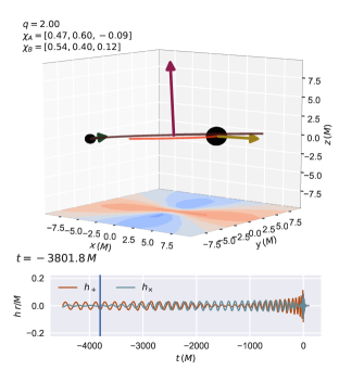
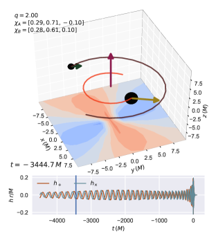
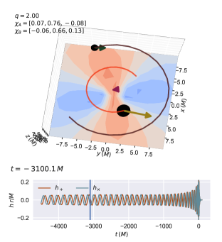
Figure 4: Visualization of a precessing binary black hole system where we also vary the camera viewing angle during the inspiral. Notice how the waveform structure in the bottom subplots changes based on whether the viewing angle is edge-on (top-left), intermediate (top-right), or face-on (bottom). This animation is available at vijayvarma392.github.io/binaryBHexp/#prec_bbh_rotating_camera.

3 Explorations

We now provide additional examples that demonstrate the power and utility of our visualizations.

3.1 Waveform projection

Figure 4 shows a visualization of a precessing binary BH, when we also vary the camera viewing angle during the evolution. The polarization content and the morphology of the waveform therefore strongly depend on the direction of the line of sight, which can be understood as follows. From Eq. (7), the observer viewing angles $(\theta,\phi)$ affect the relative weights with which the waveform modes $h_{\ell m}$ are combined into the strain $h$. Note that the standard quadrupole formula for GW emission only contains the dominant $\ell\!=\!|m|\!=\!2$ modes, while here we use all modes with $\ell\leq 4$.

The GW amplitude is strongest along the direction of $\bm{L}$. This is evident from the bottom panel of Fig. 4, where the direction of $\bm{L}$ aligns with the observer’s viewing angle (i.e., the binary is face-on). On the other hand (top-left panel of Fig. 4) the GW amplitude is at its least when the observer viewing angle is orthogonal to $\bm{L}$ (edge-on). The contribution of higher harmonics $\ell>2$ to Eq. (7) also depends on observer viewing angle. For face-on binaries, the GWs are strongly dominated by the quadrupolar modes. Going from face-on to edge-on, the contribution of the quadrupolar modes decreases and that of the nonquadrupolar modes increases.

One can also infer the polarization content of the GWs from the waveform panel. If there is a $\pm 90^{\circ}$ phase shift between $h_{+}=\Re(h)$ and $h_{\times}=-\Im(h)$, the GWs are circularly polarized. The bottom panel of Fig. 4, which is mostly face-on, shows almost perfect circular polarization, deviating due to precession of the orbital plane. For comparison, when $h_{+}$ and $h_{\times}$ are proportional with a real constant of proportionality, the GW has a linear polarization (this includes the simpler case where one of the two polarizations vanishes). The top-left panel of Fig. 4, where the system is (almost) edge-on, exhibits (almost) linear polarization at many times throughout the inspiral. Again the deviations are due to precession of the orbital plane. The modulation is more noticeable for nearly edge-on precessing systems, since one of the polarizations can temporarily vanish as the system precesses through perfectly edge-on configurations.

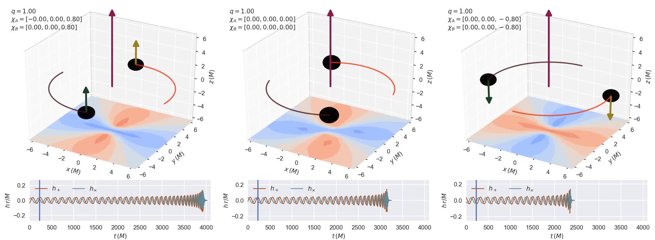
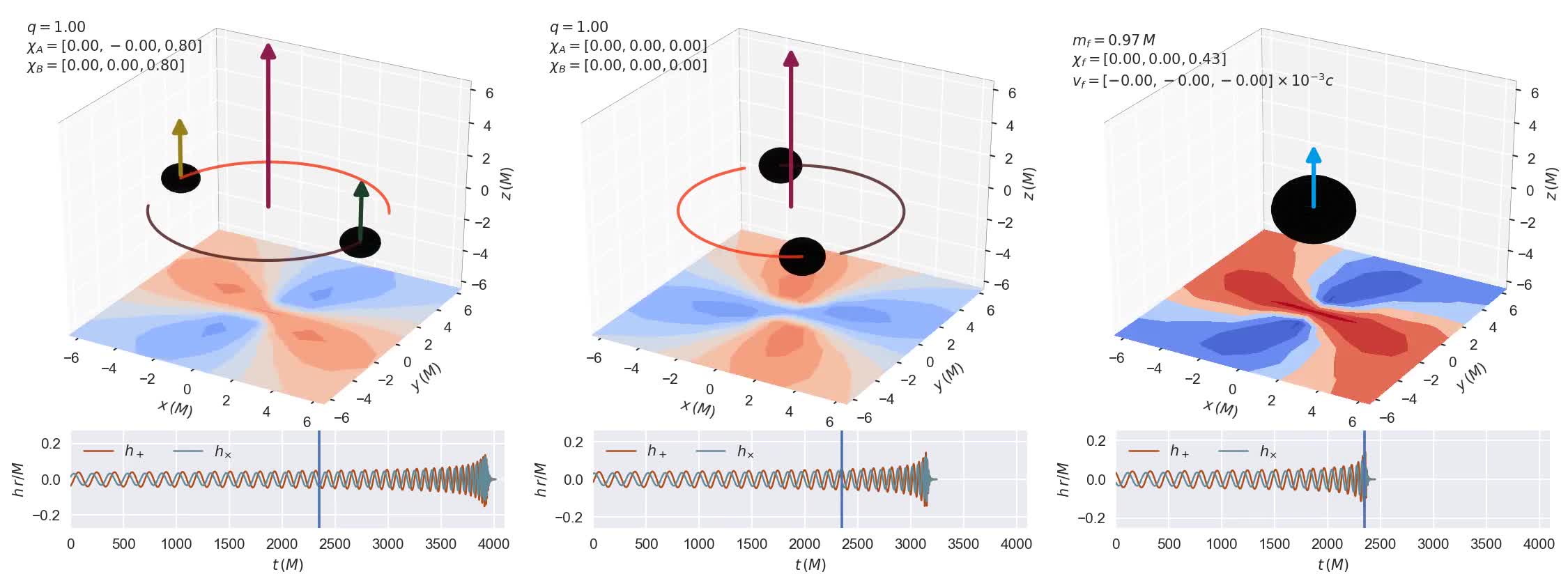
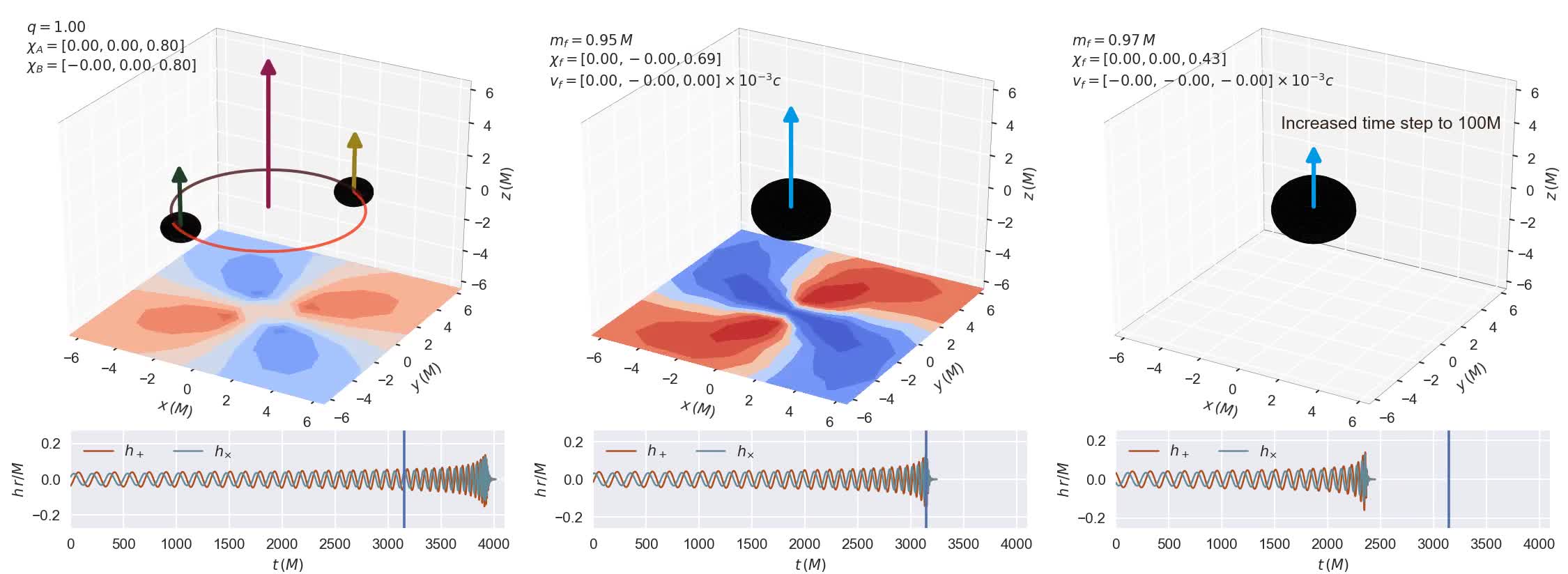
$\omega_{\text{orb}}=0.018~{}\text{rad}/M$ $t\sim 2300\,M$ $t\sim 3150\,M$ $t\sim 3950\,M$

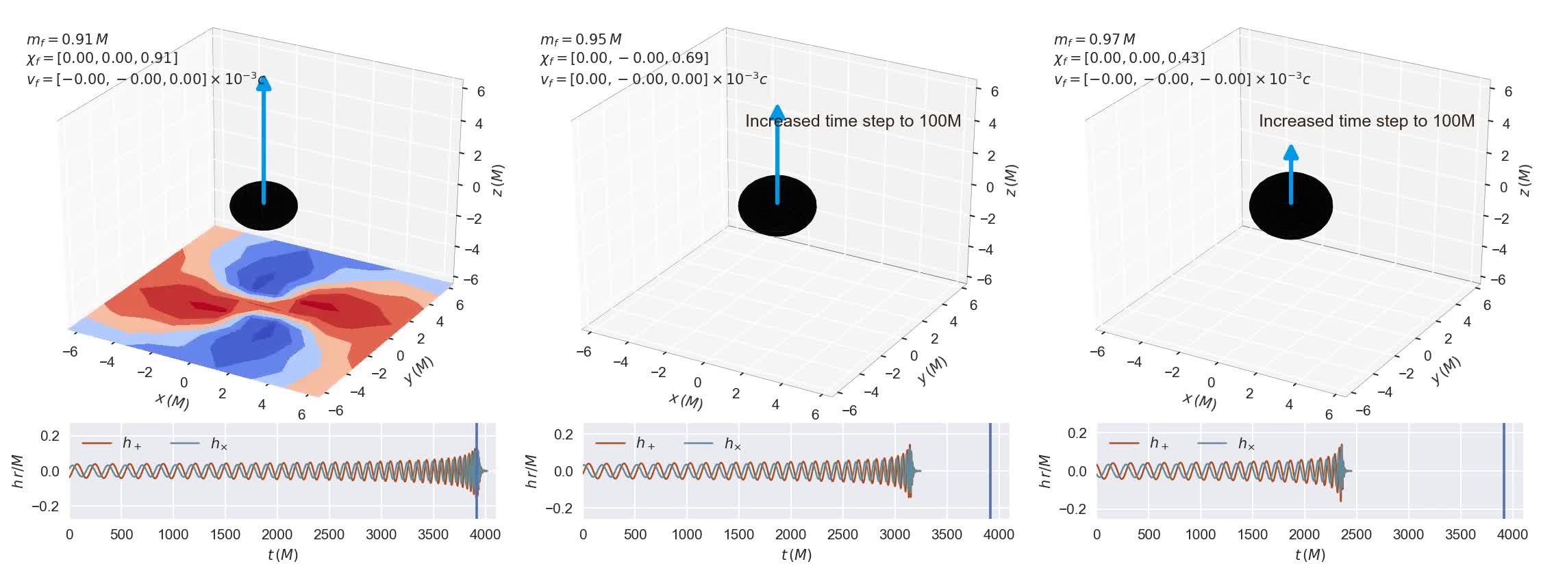
Figure 5: Visualization of the orbital hang-up effect. We show three nonprecessing systems with equal masses, and equal spins. In the left (right) column, both spins are aligned (anti-aligned) with $\bm{L}$, with magnitude 0.8. The middle column shows a nonspinning binary. All three systems start at an orbital frequency of $0.018~{}\text{rad}/M$. Due to orbital hang-up effect, the length of the waveform is longer (shorter) for the aligned case compared to the nonspinning case (see the bottom subplots showing the waveform). Time flows downwards (labeled at the left), and each row corresponds to a fixed time since the start of the animation. This animation is available at vijayvarma392.github.io/binaryBHexp/#hangup.

3.2 Orbital hang-up effect

Apart from precession, the BH spins have other important effects on the evolution of binaries. One such effect is the so called orbital hang-up effect [44, 45, 46] which delays or prompts the merger of the BHs based on the sign of the BH spin component along the orbital angular momentum, $\bm{S}\cdot\bm{L}$, where $\bm{S}$ is one of $\bm{S}_{1}$ or $\bm{S}_{2}$. This spin-orbit coupling is a $1.5$ PN effect that effectively acts as an additional repulsion (attraction) when the sign of $\bm{S}\cdot\bm{L}$ is positive (negative). This means that binaries that have spins that are aligned (anti-aligned) with $\bm{L}$ will merge slower (faster) than nonspinning binaries, when starting from the same orbital frequency. This is analogous to the location of the innermost stable circular orbits of Kerr BHs, which is at a smaller (larger) radius for co-(counter-)rotating particles.

This is demonstrated in Fig. 5, which shows an aligned, nonspinning and an anti-aligned binary, starting at the same orbital frequency. Unlike the rest of the animations discussed in this paper, here we use a constant time step between the frames of the movie (rather than a fixed 30 frames per orbit), and set $t=0$ at the start of the waveform (rather than at the peak). Due to the orbital hang-up effect, the anti-aligned binary merges first, followed by the nonspinning system, and finally the aligned system. In addition, the aligned (anti-aligned) binary radiates more (less) energy due to its prolonged (shortened) evolution, and the final mass is therefore smaller (larger) than the nonspinning case. The interaction between spin and orbital angular momentum also determines the remnant spin in a non-trivial way: the aligned (anti-aligned) case results in the largest (smallest) remnant spin magnitude.

The orbital hang-up effect can also be explained heuristically using the cosmic censorship conjecture. For the aligned-spin binary in Fig. 5, the initial magnitude of total angular momentum is given by $J=L+m_{1}^{2}~{}\chi_{1}+m_{2}^{2}~{}\chi_{2}$. Using $L$ from Eq. (2) with $\omega_{\rm orb}=0.018~{}\text{rad}/M$, we get $J\sim 1.35M^{2}$. This is larger than the maximum allowed spin angular momentum for a Kerr BH, $M^{2}$. On the other hand, for the anti-aligned case we have $J=L-m_{1}^{2}~{}\chi_{1}-m_{2}^{2}~{}\chi_{2}\sim 0.55M^{2}$, which is well within the limit. So, the aligned binary must radiate at least $0.35M^{2}$ of its total angular momentum in the form of GWs before it can merge, in order to not violate cosmic censorship. The anti-aligned case can therefore merge faster.

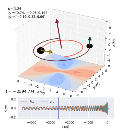
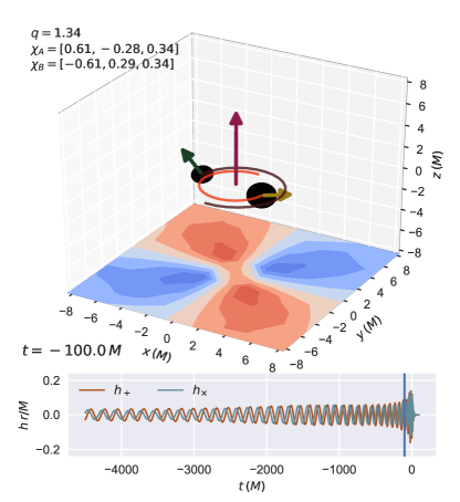
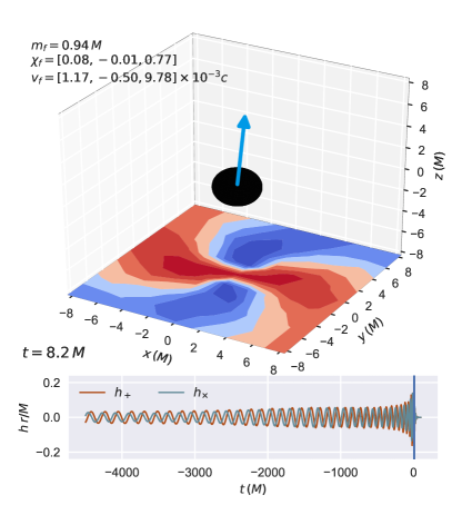
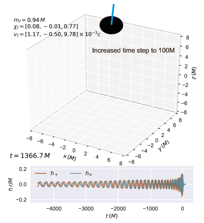
Figure 6: Evolution of a super-kick configuration. Time flows from left to right and from top to bottom, as shown at the bottom left of each panel. The top-left panel shows a snapshot taken in the early inspiral. In the top-right panel, the two BHs are about to merge and the spins are are seen to be in a super-kick configuration. The bottom-left snapshot is taken at the time at which the peak of the waveform hits the bottom plane where the GW pattern is shown. After merger (bottom-right panel), the final BH is imparted a kick of $\sim 3000$ km/s (note that we speed up the animation after the ringdown by increasing the time steps to $100M$). This animation is available at vijayvarma392.github.io/binaryBHexp/#super_kick.

3.3 Super-kick

Next, we consider a binary BH in the so-called super-kick configuration. Anisotropic emission of GWs causes a net flux of linear momentum, which imparts a kick to the remnant BH. Some degree of asymmetry is necessary for a nonzero kick [47]. For instance the kick vanishes by symmetry during the merger of an equal-mass, nonspinning binary BH system. Strongly precessing binary BHs have been found to generate the highest kicks [48, 49, 50]. Some of these systems have kicks large enough to escape from even the most massive galaxies in the Universe [51, 52].

In particular, a vary large kick (up to $\sim 3000$ km/s) is imparted to BHs merging with spins lying in the orbital plane and anti-parallel to each other. These are the so-called super-kicks first discovered in 2007 [48, 49], by means of NR simulations. The largest kicks observed in numerical simulations to date are the so-called hangup-kicks [50], where the spins have non-zero components perpendicular to the orbital plane, but the in plane spins are anti-parallel. We will refer to all configurations where the spins near merger are coplanar, and their orbital plane projections are anti-parallel, as super-kick configurations. Crucially, large kicks are only found if the spins are in these fine-tuned configurations “near merger.”

For this reason, generating visualizations of BH super-kicks from simulations can be challenging. The spins are usually specified at the start of the simulations and several attempts are necessary to find the specific initial conditions that will result in co-planar spins near merger. With our tool, on the other hand, one can specify the spins at any time/frequency, including close to merger. Generating a visualization of a system in a super-kick configuration is as easy as any other location in parameter space. This is shown in Fig. 6. The remnant reaches a final velocity of $\sim 10^{-2}c$ ($\sim 3000km/s$), in agreement with [48, 49, 50].

	$\alpha=0$	$\alpha=\frac{\pi}{4}$	$\alpha=\frac{\pi}{2}$	$\alpha=\frac{3\pi}{4}$	$\alpha=\pi$
$t=-2000M$
$t=-100M$
$t=0M$
$t=1365M$

Figure 7: Sinusoidal dependence of the kick magnitude on the angle between spins close to merger. Five different cases are shown (left to right), with equal masses and equal spins. Both spins are confined to the orbital plane, and are anti-parallel to each other, but with a different angle in the plane $\alpha$ (labeled at top), specified at $t\!=\!-100M$. Time flows downwards (labeled at left). The bottom panels show the sinusoidal dependence of the final kick magnitude on the initial orbital phase. This animation is available at vijayvarma392.github.io/binaryBHexp/#sine_kicks.

3.4 Sinusoidal kick dependence

As suggested above, the remnant kick is quite sensitive to the angle between the spins close to merger. In particular, the component of the kick parallel to the orbital angular momentum has been found to depend sinusoidally on the orbital phase [53, 38]. Fig. 7 demonstrates this effect. All five different cases have equal-mass BHs, with anti-parallel spins lying in the orbital plane at $t=-100M$. Each evolution is initialized with a different orbital phase or, equivalently, performing an overall rotation of the spins about the $z$-axis.

As expected, the final BH kick changes dramatically with the initial orbital phase. Even visually, the kick dependence appears to be sinusoidal. This example demonstrates the potential of binaryBHexp as a tool to perform detailed, but at the same time accessible, exploration of the phenomenology of precessing BH mergers.

4 Public Python implementation

Our package is made publicly available through the easy-to-install-and-use Python package, binaryBHexp [54]. Our code is compatible with both Python 2 and Python 3. The latest release can be installed from the Python Package Index using

    pip install binaryBHexp

This adds a shell command called binaryBHexp, which can be used to generate visualizations with invocation as simple as

    binaryBHexp --q 2 --chiA 0.2 0.7 -0.1 --chiB 0.2 0.6 0.1

Such an invocation yields a running movie that the user can interact with. By clicking and dragging on the movie as it plays, the user can change the viewing angle and the waveform time-series will update in real time as the viewing angle is manipulated. The full documentation for command-line arguments is available with the --help flag.

As mentioned in Sec. 2.5, the default setting for the spin arrows is to be proportional to the Kerr parameter of the BH, $a$. By passing the optional argument --use_spin_angular_momentum_for_arrows to the above command, the spin arrows can be made proportional to the spin angular momentum of the BH instead.

Python packages NRSur7dq2 [55] and surfinBH [56] are specified as dependencies and are automatically installed by pip if missing. binaryBHexp is hosted on GitHub at github.com/vijayvarma392/binaryBHexp, from which development versions can be installed. Continuous integration is provided by Travis [57]. More details about the Python implementation, as well as animations corresponding to the examples discussed in this paper are available at vijayvarma392.github.io/binaryBHexp.

5 Conclusion

We present a tool for visualizing mergers of precessing binary black holes. Rather than rely on expensive numerical simulations, we base our animations on surrogate models of numerical simulations. These are inexpensive but very accurately reproduce numerical simulations. Therefore, we can generate visualizations anywhere in the parameter space of the underlying surrogate models, within a few seconds.

We make our code available through an easy-to-install-and-use python package binaryBHexp [54]. We demonstrate the power of this tool by generating visualizations of several well known phenomena such as: spin and waveform modulations due to precession, orbital-hangup effect, super kicks, sinusoidal behavior of the remnant kick, etc. This tool can be used by researchers and students alike, to gain valuable insights into the highly complex dynamics of precessing binary black holes.

References

- [1] Abbott B P et al. (LIGO Scientific Collaboration, Virgo Collaboration) 2016 Phys. Rev. Lett. 116(6) 061102 [arXiv:1602.03837]
- [2] Aasi J et al. (LIGO Scientific Collaboration) 2015 Class. Quantum Grav. 32 074001 [arXiv:1411.4547]
- [3] nobelprize.org/prizes/physics/2017
- [4] Apostolatos T A, Cutler C, Sussman G J and Thorne K S 1994 Phys. Rev. D49 6274–6297
- [5] Kidder L E 1995 Phys. Rev. D52 821–847 [arXiv:gr-qc/9506022]
- [6] Racine E 2008 Phys. Rev. D78 044021 [arXiv:0803.1820]
- [7] Gerosa D, Kesden M, Sperhake U, Berti E and O’Shaughnessy R 2015 Phys. Rev. D 92 064016 [arXiv:1506.03492]
- [8] Acernese F et al. (Virgo Collaboration) 2015 Class. Quantum Grav. 32 024001 [arXiv:1408.3978]
- [9] Lehner L and Pretorius F 2014 Ann. Rev. Astron. Astrophys. 52 661–694 [arXiv:1405.4840]
-
[10]
SXS:
youtube.com/user/SXSCollaboration,
LIGO Lab:youtube.com/channel/UC4oFlSYpDywInX0lxpiBPwA,
AEI: youtube.com/channel/UCw6knnFFBhdnwylMohte45A,
LIGO/Virgo: youtube.com/channel/UCMATJmzibndbcdY8s9Prhjg. - [11] Blackman J, Field S E, Scheel M A, Galley C R, Ott C D, Boyle M, Kidder L E, Pfeiffer H P and Szilágyi B 2017 Phys. Rev. D96 024058 [arXiv:1705.07089]
- [12] Varma V, Gerosa D, Stein L C, Hébert F and Zhang H 2019 Phys. Rev. Lett. 122 011101 [arXiv:1809.09125]
- [13] Schutz B F 2009 A First Course in General Relativity 2nd ed (New York: Cambridge University Press)
- [14] Maggiore M 2008 Gravitational Waves - Volume 1 1st ed (New York, NY: Oxford University Press)
- [15] Baumgarte T W and Shapiro S L 2010 Numerical Relativity: Solving Einstein’s Equations on the Computer (New York: Cambridge University Press)
- [16] Hartle J B 2003 Gravity: An Introduction to Einstein’s General Relativity (New York: Addison-Wesley)
- [17] Carroll S 2003 Spacetime and Geometry: An Introduction to General Relativity (New York: Addison Wesley)
- [18] Misner C W, Thorne K S and Wheeler J A 1973 Gravitation (New York, New York: Freeman)
- [19] Boyle M, Owen R and Pfeiffer H P 2011 Phys. Rev. D 84 124011 [arXiv:arXiv:1110.2965 [gr-qc]]
- [20] Schmidt P, Hannam M, Husa S and Ajith P 2011 Phys. Rev. D84 024046 [arXiv:1012.2879]
- [21] O’Shaughnessy R, Vaishnav B, Healy J, Meeks Z and Shoemaker D 2011 Phys. Rev. D84 124002 [arXiv:1109.5224]
- [22] Visser M 2007 The Kerr spacetime: A Brief introduction Kerr Fest: Black Holes in Astrophysics, General Relativity and Quantum Gravity Christchurch, New Zealand, August 26-28, 2004 [arXiv:0706.0622]
- [23] Bohn A, Kidder L E and Teukolsky S A 2016 Phys. Rev. D94 064008 [arXiv:1606.00437]
- [24] Bohn A, Kidder L E and Teukolsky S A 2016 Phys. Rev. D94 064009 [arXiv:1606.00436]
-
[25]
youtube.com/watch?v=Tr1zDVbSjTM,
youtube.com/watch?v=9HKh4ADvMoA,
youtube.com/watch?v=CeNP5NyW0z4. - [26] Poisson E and Sasaki M 1995 Phys. Rev. D51 5753–5767 [arXiv:gr-qc/9412027]
- [27] Alvi K 2001 Phys. Rev. D64 104020 [arXiv:gr-qc/0107080]
- [28] Poisson E 2004 Phys. Rev. D70 084044 [arXiv:gr-qc/0407050]
- [29] Zhao X, Kesden M and Gerosa D 2017 Phys. Rev. D96 024007 [arXiv:1705.02369]
- [30] Schnittman J D 2004 PRD 70 124020 [arXiv:astro-ph/0409174]
- [31] Lousto C O and Healy J 2015 Physical Review Letters 114 141101 [arXiv:1410.3830]
- [32] Gerosa D, Lima A, Berti E, Sperhake U, Kesden M and O’Shaughnessy R 2018 arXiv e-prints [arXiv:1811.05979]
- [33] Gerosa D, Kesden M, O’Shaughnessy R, Klein A, Berti E, Sperhake U and Trifirò D 2015 Physical Review Letters 115 141102 [arXiv:1506.09116]
- [34] Afle C, Gupta A, Gadre B, Kumar P, Demos N, Lovelace G, Choi H G, Lee H M, Mitra S, Boyle M, Hemberger D A, Kidder L E, Pfeiffer H P, Scheel M A and Szilagyi B 2018 PRD 98 083014 [arXiv:1803.07695]
- [35] Ossokine S et al. 2019 In preparation
- [36] Varma V, Field S E, Scheel M A, Blackman J, Kidder L E and Pfeiffer H P 2019 Phys. Rev. D99 064045 [arXiv:1812.07865]
- [37] Bohe A, Marsat S, Faye G and Blanchet L 2013 Class. Quantum Grav. 30 075017 [arXiv:1212.5520]
- [38] Gerosa D, Hébert F and Stein L C 2018 Phys. Rev. D97 104049 [arXiv:1802.04276]
- [39] Boyle M 2013 Phys. Rev. D87 104006 [arXiv:1302.2919]
- [40] Szilágyi B, Lindblom L and Scheel M A 2009 Phys. Rev. D 80 124010 [arXiv:0909.3557]
- [41] Flanagan E E and Hughes S A 2005 New J. Phys. 7 204 [arXiv:gr-qc/0501041]
- [42] Goldberg J N, Macfarlane A J, Newman E T, Rohrlich F and Sudarshan E C G 1967 Journal of Mathematical Physics 8 2155–2161
- [43] Thorne K S 1980 Rev. Mod. Phys. 52 299–339
- [44] Damour T 2001 Phys. Rev. D64 124013 [arXiv:gr-qc/0103018]
- [45] Campanelli M, Lousto C O and Zlochower Y 2006 Phys. Rev. D74 041501 [arXiv:gr-qc/0604012]
- [46] Scheel M A, Giesler M, Hemberger D A, Lovelace G, Kuper K, Boyle M, Szilágyi B and Kidder L E 2015 Class. Quant. Grav. 32 105009 [arXiv:1412.1803]
- [47] Boyle L, Kesden M and Nissanke S 2008 Phys. Rev. Lett. 100 151101 [arXiv:0709.0299]
- [48] Campanelli M, Lousto C O, Zlochower Y and Merritt D 2007 Astrophys. J. 659 L5–L8 [arXiv:gr-qc/0701164]
- [49] Gonzalez J A, Hannam M D, Sperhake U, Bruegmann B and Husa S 2007 Phys. Rev. Lett. 98 231101 [arXiv:gr-qc/0702052]
- [50] Lousto C O and Zlochower Y 2011 Phys. Rev. Lett. 107 231102 [arXiv:1108.2009]
- [51] Merritt D, Milosavljevic M, Favata M, Hughes S A and Holz D E 2004 Astrophys. J. 607 L9–L12 [arXiv:astro-ph/0402057]
- [52] Gerosa D and Sesana A 2015 Mon. Not. Roy. Astron. Soc. 446 38–55 [arXiv:1405.2072]
- [53] Brügmann B, González J A, Hannam M, Husa S and Sperhake U 2008 Phys. Rev. D 77 124047 [arXiv:arXiv:0707.0135]
-
[54]
binaryBHexp. Website:
vijayvarma392.github.io/binaryBHexp,
Python package: pypi.org/project/binaryBHexp,
Code repository: github.com/vijayvarma392/binaryBHexp. - [55] Blackman J et al. pypi.org/project/NRSur7dq2
- [56] Varma V et al. pypi.org/project/surfinBH, doi.org/10.5281/zenodo.1418525
- [57] Travis Continuous Integration travis-ci.org