The Orbital Parameters of the Eclipsing High-Mass X-ray Binary Pulsar IGR J16493–4348 from Pulsar Timing

Abstract

IGR J16493–4348 is an eclipsing supergiant high-mass X-ray binary (sgHMXB), where accretion onto the compact object occurs via the radially outflowing stellar wind of its early B-type companion. We present an analysis of the system’s X-ray variability and periodic modulation using pointed observations (2.5–25 keV) and Galactic bulge scans (2–10 keV) from the Rossi X-ray Timing Explorer (RXTE) Proportional Counter Array (PCA), along with Swift Burst Alert Telescope (BAT) 70-month snapshot (14–195 keV) and transient monitor (15–50 keV) observations. The orbital eclipse profiles in the PCA bulge scans and BAT light curves are modeled using asymmetric and symmetric step and ramp functions. We obtain an improved orbital period measurement of 6.7828 $\pm$ 0.0004 days from an observed minus calculated (O–C) analysis of mid-eclipse times derived from the BAT transient monitor and PCA scan data. No evidence is found for the presence of a strong photoionization or accretion wake. We refine the superorbital period to 20.067 $\pm$ 0.009 days from the discrete Fourier transform (DFT) of the BAT transient monitor light curve. A pulse period of 1093.1036 $\pm$ 0.0004 s is measured from a pulsar timing analysis using pointed PCA observations spanning $\sim$1.4 binary orbits. We present pulse times of arrival (ToAs), circular and eccentric timing models, and calculations of the system’s Keplerian binary orbital parameters. We derive an X-ray mass function of $f_{x}(M)$ $=$ 13.2${}^{\text{+2.4}}_{\text{--2.5}}$ $M_{\odot}$ and find a spectral type of B0.5 Ia for the supergiant companion through constraints on the mass and radius of the donor. Measurements of the eclipse half-angle and additional parameters describing the system geometry are provided.

${}^{\text{1}}$ Division of Physics, Mathematics, and Astronomy, California Institute of Technology, Pasadena, CA 91125, USA; aaron.b.pearlman@caltech.edu
${}^{\text{2}}$ Department of Physics and Astronomy, Howard University, Washington, DC 20059, USA
${}^{\text{3}}$ CRESST/Mail Code 661, Astroparticle Physics Laboratory, NASA Goddard Space Flight Center, Greenbelt, MD 20771, USA
${}^{\text{4}}$ CRESST/Mail Code 662, X-ray Astrophysics Laboratory, NASA Goddard Space Flight Center, Greenbelt, MD 20771, USA
${}^{\text{5}}$ University of Maryland, Baltimore County, Baltimore, MD 21250, USA

1. Introduction

IGR J16493–4348 is a persistently accreting supergiant high-mass X-ray binary (sgHMXB), where mass transfer onto the neutron star is driven by the stellar wind from its early B-type companion. It was first detected during a survey of the Galactic plane (Bird et al., 2004) using the INTErnational Gamma-Ray Astrophysics Laboratory (INTEGRAL; Winkler et al. 2003) with the INTEGRAL Soft Gamma-Ray Imager (ISGRI; Lebrun et al. 2003) camera of the Imager on Board the INTEGRAL Satellite (IBIS; Ubertini et al. 2003) telescope. The source was also detected with INTEGRAL during a deep scan of the Norma Arm region (Grebenev et al., 2005) and in subsequent IBIS/ISGRI (Bird et al., 2006, 2007, 2010, 2016) and Swift Burst Alert Telescope (BAT) surveys (Baumgartner et al., 2013; Oh et al., 2018).

Pointed Rossi X-ray Timing Explorer (RXTE) Proportional Counter Array (PCA) observations of IGR J16493–4348 by Markwardt et al. (2005) revealed that the mean spectrum was consistent with a heavily absorbed power law, with a photon index of $\Gamma$ $=$ 1.4 and $N_{\text{H}}$ $\approx$ 10${}^{\text{23}}$ cm${}^{\text{--2}}$. The measured fluxes in the 2–10, 10–20, and 20–40 keV energy bands were 1.0 $\times$ 10${}^{\text{--11}}$, 1.3 $\times$ 10${}^{\text{--11}}$, and 2.1 $\times$ 10${}^{\text{--11}}$ erg cm${}^{\text{--2}}$ s${}^{\text{--1}}$, respectively. Chandra imaging of the field of IGR J16493–4348 was performed by Kuiper et al. (2005) using the High Resolution Camera (HRC-I) instrument, which identified 2MASS J16492695–4349090 as the infrared counterpart. A $K_{\text{S}}$ magnitude of 12.0 $\pm$ 0.1 was found using the Son of ISAAC (SOFI) infrared camera at the European Southern Observatory (ESO) 3.5 m New Technology Telescope (NTT), which is consistent with the 11.94 $\pm$ 0.04 $K_{\text{S}}$ magnitude reported in the 2MASS catalog and suggests that the source is not highly variable in this band. No optical counterpart was found in the Digital Sky Survey (DSS) maps due to strong absorption along the line of sight.

A spectral type of B0.5-1 Ia-Ib was estimated by Nespoli et al. (2008, 2010) from $K_{\text{S}}$-band spectroscopy of IGR J16493–4348’s infrared counterpart using observations from the Infrared Spectrometer and Array Camera (ISAAC) spectrograph on UT1 of the ESO Very Large Telescope (VLT). The spectrum showed a strong He I (20581 Å) emission line with He I (21126 Å) in absorption, along with a strong Br$\gamma$ (21661 Å) absorption line, which are all characteristic features in OB stellar spectra. This led Nespoli et al. (2008, 2010) to classify the system as an sgHMXB. They also provided an estimate of the interstellar extinction and calculated a hydrogen column density of $N_{\text{H}}$ $=$ (2.92 $\pm$ 1.96) $\times$ 10${}^{\text{22}}$ cm${}^{\text{--2}}$, which they attributed to a significant absorbing envelope surrounding the neutron star. The distance to the source was estimated to be between 6–26 kpc. Romano (2015) found that the cumulative luminosity distribution (CLD) and small dynamic range in X-ray flux from Swift X-ray Telescope (XRT) observations were also typical of a classical sgHMXB system, rather than a Supergiant Fast X-ray Transient (SFXT).

Hill et al. (2008) carried out a spectral analysis of the source using 22–100 keV INTEGRAL IBIS/ISGRI and 1–9 keV Swift XRT data. They found that the source was best modeled by a highly absorbed power law, with $\Gamma$ $=$ 0.6 $\pm$ 0.3 and $N_{\text{H}}$ $=$ 5.4${}^{\text{+1.3}}_{\text{--1.0}}$ $\times$ 10${}^{\text{22}}$ cm${}^{\text{--2}}$, and a high energy cut-off at $E_{\text{cut}}$ $=$ 17${}^{\text{+5}}_{\text{--3}}$ keV. An average source flux of 1.1 $\times$ 10${}^{\text{--10}}$ erg cm${}^{\text{--2}}$ s${}^{\text{--1}}$ was measured in the 1–100 keV energy band. No coherent periodicities were found in their INTEGRAL or Swift data.

Morris et al. (2009) analyzed the 0.2–150.0 keV spectrum of IGR J16493–4348 obtained from Suzaku observations with the Hard X-ray Detector (HXD) and X-ray Imaging Spectrometer (XIS) instruments. The spectrum was fit with a power law modified by a fully and partially covering absorber. The partially covered and fully covered neutral hydrogen column densities were 26${}^{\text{+9.4}}_{\text{--7.9}}$ $\times$ 10${}^{\text{22}}$ and 8.6${}^{\text{+0.9}}_{\text{--1.0}}$ $\times$ 10${}^{\text{22}}$ cm${}^{\text{--2}}$, respectively, with a partial covering fraction of 0.62${}^{\text{+0.06}}_{\text{--0.07}}$ and photon index of $\Gamma$ $=$ 2.4 $\pm$ 0.2. A 6.4 keV Fe emission line, with an equivalent width less than 84 eV, was also included in their spectral model, and a flux of 13.5${}^{\text{+0.3}}_{\text{--2.0}}$ $\times$ 10${}^{\text{--12}}$ erg cm${}^{\text{--2}}$ s${}^{\text{--1}}$ was measured between 0.2 and 10 keV.

Spectral analysis in the hard X-ray band was also performed by D’Aì et al. (2011) using 15–150 keV Swift BAT and INTEGRAL/ISGRI data, together with pointed soft X-ray observations from Suzaku and the Swift XRT. They found that a negative-positive exponential power law model, with a broad (10 keV width) absorption line at 33 $\pm$ 4 keV, yielded the best fit to the broadband spectrum. This absorption feature was interpreted as evidence of a cyclotron resonance scattering feature (CRSF). Assuming cyclotron absorption occurs above the magnetic poles of the neutron star, D’Aì et al. (2011) inferred a surface magnetic field of $B_{\text{surf}}$ $=$ (3.7 $\pm$ 0.4) $\times$ 10${}^{\text{12}}$ G from the energy of the cyclotron line for a canonical neutron star with a mass of 1.4 $M_{\odot}$ and a radius of 10 km.

The 6.8 day binary orbital period was independently discovered by Corbet et al. (2010a) and Cusumano et al. (2010). Cusumano et al. (2010) also found evidence of an eclipse in the folded Swift BAT survey light curve lasting approximately 0.8 days. Assuming a neutron star mass of 1.4 $M_{\odot}$ and a B0.5 Ib companion with a mass and radius of 47 $M_{\odot}$ and 32.2 $R_{\odot}$, respectively, Cusumano et al. (2010) estimated a semi-major axis of $a$ $\approx$ 55 $R_{\odot}$ for the binary orbit and derived an upper limit of $e$ $\leq$ 0.15 on the eccentricity.

A 20 day superorbital period was first detected by Corbet et al. (2010a) in the power spectra of the Swift BAT survey and RXTE PCA scan light curves. The superorbital period was refined to 20.07 $\pm$ 0.01 days using data from the Swift BAT transient monitor (15–50 keV), and a monotonic relationship between the superorbital and orbital modulation was suggested (Corbet & Krimm, 2013). Recently, Coley et al. (2018) analyzed Nuclear Spectroscopic Telescope Array (NuSTAR) and Swift XRT observations near the maximum and minimum of one cycle of the 20 day superorbital modulation. They found that the 3–40 keV spectra were well modeled by an absorbed power law, with $N_{\text{H}}$ $\approx$ 10${}^{\text{23}}$ cm${}^{\text{--2}}$, and a high energy cut-off. Evidence of an Fe K$\alpha$ emission line was also found at superorbital maximum near 6.4 keV. A comprehensive discussion of possible mechanisms responsible for the superorbital variability is presented in Coley et al. (2018), along with a timing analysis characterizing its long term behavior.

A 1069 s period was detected in the power spectrum of the light curve from pointed RXTE PCA observations, which was suggested to be linked to the neutron star’s rotational period (Corbet et al., 2010b). We find strong evidence for a 1093 s pulse period from pulsar timing measurements using additional archival pointed RXTE PCA observations. Pulse phase resolved spectroscopy near the maximum and minimum of the superorbital cycle has recently been carried out by Coley et al. (2018) using these pulsar timing results.

In this paper, we present improved measurements of IGR J16493–4348’s superorbital, orbital, and pulse periods using Swift BAT and RXTE PCA observations. We also measure the system’s Keplerian binary orbital parameters and study the nature of the supergiant donor and the geometry of the binary. The observations and our data reduction procedure are described in Section 2. In Section 3, we provide refined period measurements and model the system’s eclipse profile. A pulsar timing analysis is presented in Sections 4.1–4.3, along with pulse times of arrival (ToAs) and orbital timing models. New constraints on the spectral type of the supergiant donor and possible system geometries are given in Section 4.4. A discussion of the spectral type of the supergiant companion, eclipse asymmetries, orbital eccentricity, and possible superorbital mechanisms is provided in Section 5. We summarize our results and conclusions in Section 6.

2. Observations

2.1. RXTE PCA Pointed Observations

The PCA (Jahoda et al., 1996, 2006) was the primary instrument on board the RXTE satellite. The detector was comprised of five nearly identical Proportional Counter Units (PCUs), with a total effective area of $\sim$6500 cm${}^{\text{2}}$, and was sensitive to X-rays with energies between 2 and 60 keV. The mechanically collimated array had a 1^∘ field of view (FoV) at full width at half maximum (FWHM). Each PCU had a multi-anode main volume filled with xenon and methane and a front propane-filled “veto” volume that was used primarily for background rejection.

We analyzed 24 pointed RXTE PCA observations collected at $\sim$0.4 day intervals during 2011 October, which spanned $\sim$9.5 days. The total exposure time was $\sim$160.5 ks, and the exposure times of individual observations ranged between 1.7 and 16.0 ks. A catalog of these observations is provided in Table 1, and they are accessible through the High Energy Astrophysics Science Archive Research Center (HEASARC) archive.

Background-subtracted PCA light curves were created using the Standard 2 mode and FTOOLS v6.22 (Blackburn, 1995). The time resolution of the light curves was 16 s, and we used data obtained from the top xenon layers (1L and 1R) of the PCUs to maximize the signal-to-noise ratio. The Faint background model was used to background subtract all of the PCA data since the net count rate did not exceed 40 counts s${}^{\text{--1}}$ PCU${}^{\text{--1}}$. To reduce the uncertainty of the PCA background model, we excluded data: (1) up to 10 minutes immediately following the peak of South Atlantic Anomaly (SAA) passages, (2) with an elevation angle less than 10^∘ above the limb of the Earth, (3) with an electron ratio larger than 0.1 in at least one of the operating PCUs, indicating high electron contamination according to the ratio of veto rates in the detectors, (4) with an offset between the source position and RXTE’s pointing position larger than 0.01^∘, and (5) within 150 s of the start of a PCU breakdown event and up to 600 s following a PCU breakdown event using the PCA breakdown history. A detailed discussion of PCA calibration issues was provided by Jahoda et al. (2006). The light curve times were corrected to the solar system barycenter using the faxbary FTOOLS routine and the Jet Propulsion Laboratory (JPL) DE-200 ephemeris (Standish, 1990). Throughout this paper, Modified Julian Dates (MJDs) refer to the barycentric times.

Data from all available PCUs were used during each pointed observation. The RXTE PCA (2.5–25 keV) light curve is shown in Figure 1 with count rates normalized by the number of operational PCUs. Orbital phase 0 corresponds to $T_{\pi/2}$ from circular solution 1 in Table 6. In Figure 2(d), we show the pointed RXTE PCA (2–10 keV) light curve, produced using the same data filtering criteria and 128 s time resolution, with nearly simultaneous PCA scan (2–10 keV) observations overlaid in blue.

Table 1RXTE PCA Pointed Observations of IGR J16493–4348

Observation ID	Date	Observation Timea	Time Span	Exposure Time	Count Rateb	Orbital Phasec
	(UTC)	(MJD)	(ks)	(ks)	(Counts s${}^{\text{--1}}$ PCU${}^{\text{--1}}$)
96358-01-01-01	2011 Oct 09.09–09.19	55843.13981	8.42	5.09	8.04	–1.145
96358-01-01-02	2011 Oct 09.87–09.90	55843.88558	1.87	1.87	2.94	–1.036
96358-01-01-12	2011 Oct 10.07–10.17	55844.11862	8.29	4.91	3.50	–1.001
96358-01-01-03	2011 Oct 10.48–10.57	55844.52174	8.00	5.84	3.44	–0.942
96358-01-01-04	2011 Oct 11.18–11.28	55845.23159	8.85	6.05	6.73	–0.837
96358-01-01-05	2011 Oct 11.44–11.48	55845.46157	3.44	3.44	7.35	–0.803
96358-01-01-00	2011 Oct 11.51–11.61	55845.55934	9.07	6.88	6.31	–0.789
96358-01-01-06	2011 Oct 11.64–11.68	55845.65720	3.42	3.42	5.57	–0.774
96358-01-01-07	2011 Oct 12.09–12.12	55846.10809	2.37	1.71	5.06	–0.708
96358-01-01-08	2011 Oct 12.18–12.33	55846.25345	13.12	7.68	5.22	–0.686
96358-01-01-09	2011 Oct 12.42–12.53	55846.47288	9.02	6.78	5.10	–0.654
96358-01-01-10	2011 Oct 13.27–13.37	55847.32124	9.01	6.72	6.37	–0.529
96358-01-01-11	2011 Oct 13.60–13.70	55847.64742	8.99	6.70	4.63	–0.481
96358-01-02-00	2011 Oct 14.18–14.35	55848.26709	14.61	9.34	4.37	–0.390
96358-01-02-01	2011 Oct 14.44–14.68	55848.56078	20.24	13.29	5.92	–0.346
96358-01-02-02	2011 Oct 15.16–15.33	55849.24572	14.57	9.14	6.36	–0.245
96358-01-02-03	2011 Oct 15.42–15.58	55849.50098	13.57	8.90	6.03	–0.208
96358-01-02-04	2011 Oct 16.14–16.31	55850.22417	14.54	8.83	6.64	–0.101
96358-01-02-05	2011 Oct 16.47–16.63	55850.55044	14.54	9.82	4.89	–0.053
96358-01-02-06	2011 Oct 17.18–17.48	55851.33335	25.81	15.95	3.73	0.063
96358-01-02-09	2011 Oct 17.97–17.99	55851.97617	1.66	1.66	6.56	0.157
96358-01-02-10	2011 Oct 18.03–18.06	55852.04394	2.08	2.08	5.89	0.167
96358-01-02-07	2011 Oct 18.16–18.40	55852.27911	20.16	12.50	7.13	0.202
96358-01-02-08	2011 Oct 18.55–18.58	55852.56585	2.10	1.89	9.55	0.244

Note. — Observation IDs in bold were excluded from the pulsar timing analysis since pulsed emission was not strongly detected (see also Figure 1).

^a Mid-time of observation.

^b Average 2.5–25 keV count rate after background subtraction using all available PCUs.

^c Orbital phase at the observation mid-time using the refined 6.7828 day orbital period measurement in Section 3.2.1. Phase 0 corresponds to $T_{\pi/2}$ from circular solution 1 in Table 6.

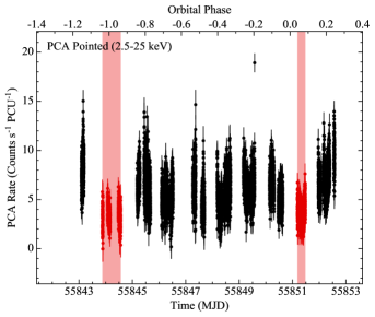
Figure 1.— Background-subtracted pointed RXTE PCA (2.5–25 keV) light curve of IGR J16493–4348 using all available PCUs with 16 s time resolution. Orbital phase 0 corresponds to $T_{\pi/2}$ from circular solution 1 in Table 6. Data plotted in red were excluded from the pulsar timing analysis since pulsations were not strongly detected.

2.2. RXTE PCA Galactic Bulge Scans

From 1999 February to 2011 November, RXTE performed raster scans of an approximately 16^∘ $\times$ 16^∘ rectangular region near the Galactic Center (GC) using the PCA (Swank & Markwardt, 2001). The count rates were modulated by the 1^∘ collimators as the source moved into and out of the PCA’s FoV during the Galactic bulge scans. These observations were carried out twice weekly, excluding November–January and June when the positions of the Sun and anti-Sun crossed the GC region. A single scan of a source had a typical exposure time of approximately 20 s per observation and was sensitive to 0.5–1 mCrab variations in the source flux. The light curves were generated in the 2–10 keV energy band using only the top layer of the PCA to optimize detections of faint sources. We corrected the light curve times to the solar system barycenter using the tools available through the Ohio State University (OSU) Department of Astronomy website (Eastman et al., 2010).

We present 524 measurements from a series of PCA Galactic bulge scans between MJDs 53163.8 and 55863.4 (2004 June 7–2011 October 29). The PCA scan (2–10 keV) weighted average light curve is shown in Figure 2(a). The Galactic bulge scan data are publicly available.

2.3. Swift BAT

The Swift BAT (Barthelmy et al., 2005; Gehrels et al., 2004) is a wide FoV (1.4 sr half-coded), hard X-ray telescope that uses a 2.7 m${}^{\text{2}}$ coded-aperture mask and is sensitive to X-rays in the 14–195 keV band. Although the BAT is primarily designed for studying gamma-ray bursts and their afterglows, it also serves as a hard X-ray transient monitor (Krimm et al., 2013) and surveys the hard X-ray sky with $\sim$0.4 mCrab sensitivity (Baumgartner et al., 2013). Thus, BAT observations of X-ray sources are usually performed in an unpredictable and serendipitous manner. Due to the nonuniform nature of the BAT sky survey, the signal-to-noise ratio of a source during an observation depends strongly on the location of the source within the BAT’s FoV. The BAT typically covers 50–80% of the sky each day. The data reduction procedures are described in detail in Krimm et al. (2013) and Baumgartner et al. (2013).

We analyzed the BAT 70-month snapshot (14–195 keV) light curve, which is shown in Figure 2(b) and spans MJDs 53360.0 through 55470.0 (2004 December 21–2010 October 1). The light curve is comprised of continuous, individual observations pointed at the same sky location. Exposure times ranged from 150 to 2679 s, and the mean exposure time was 783 s. The time resolution is determined by the sampling of the individual observations.

We also analyzed the BAT transient monitor (15–50 keV) light curve between MJDs 53416.0 and 57249.8 (2005 February 15–2015 August 15), which is shown in Figure 2(c). Orbital and daily averaged light curves are available through the Swift NASA Goddard Space Flight Center (GSFC) website after they have been processed with the data reduction procedures described in Krimm et al. (2013). We used the orbital light curve in our analysis, which had typical exposure times ranging from 64 to 2640 s and a mean exposure time of 720 s. We excluded “bad” times from the light curve, which were indicated by nonzero data quality flag (DATA_FLAG) values. A small number of data points with very low fluxes and unusually small uncertainties were also identified and removed, even though they were flagged as “good” (Corbet & Krimm, 2013). The BAT 70-month snapshot and transient monitor light curve times were corrected to the solar system barycenter using the tools available through the OSU Department of Astronomy website¹².

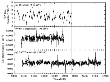
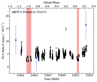
Figure 2.— (a) RXTE PCA scan (2–10 keV) weighted average light curve of IGR J16493–4348 using 30 day bin widths. (b) Swift BAT 70-month snapshot (14–195 keV) and (c) Swift BAT transient monitor (15–50 keV) weighted average light curves of IGR J16493–4348 using bin widths equal to twice the 6.7828 day orbital period. The horizontal uncertainties in Figures 2(a)–(c) correspond to the half bin widths in the light curves, and the vertical uncertainties are obtained from the standard error. The pointed PCA observation times are indicated by the blue shaded regions (smaller than the symbol size) in Figures 2(a)–(c). (d) Background-subtracted pointed RXTE PCA (2–10 keV) light curve of IGR J16493–4348 using all operational PCUs with 128 s time resolution. The red shaded regions correspond to observation times with weak pulsed emission, and nearly simultaneous RXTE PCA scan (2–10 keV) observations are overlaid as blue squares. Orbital phase 0 corresponds to $T_{\pi/2}$ from circular solution 1 in Table 6.

3. Period Measurements

The RXTE PCA scan and Swift BAT light curves were used to search for orbital and superorbital modulation since they were longer in duration. A refined superorbital period measurement was obtained from the semi-weighted discrete Fourier transform (DFT) of the BAT transient monitor light curve (see Section 3.1). In this paper, uncertainties on period measurements obtained from DFTs were determined according to Horne & Baliunas (1986). We report an improved orbital period from an observed minus calculated (O–C) analysis of mid-eclipse times derived from the BAT transient monitor and PCA scan light curves using a Bayesian Markov chain Monte Carlo (MCMC) fitting procedure (see Section 3.2.1). Pulsations were detected in the unweighted power spectrum of the pointed PCA light curve after the removal of low frequency noise (see Section 3.3). We refine the pulse period using the ToAs derived from the pulsar timing analysis described in Sections 4.1–4.3.

3.1. Superorbital Period

We searched for orbital and superorbital modulation between 1 and 100 days in the power spectra of the PCA scan, BAT 70-month snapshot, and BAT transient monitor light curves shown in Figure 3. Each of these power spectra was oversampled by a factor of five compared to their nominal frequency resolution, given by the length of the light curve.

The measurements from the PCA scan and BAT light curves showed a wide range of nonuniform error bar sizes. It can be advantageous to use these errors to weight the contribution of each data point when calculating the power spectrum (Scargle, 1989). The semi-weighting technique uses the error bar of each data point and the excess light curve variability to weight the data points in the power spectrum, which is analogous to a semi-weighted mean (Cochran, 1937, 1954). Corbet et al. (2007a, b) showed that semi-weighting can be very beneficial for faint sources, such as IGR J16493-4348. We used semi-weighting in all of the power spectra in Figure 3 since it yielded more significant period detections with smaller uncertainties.

Strong evidence of superorbital modulation near 20.07 days was found in the power spectra of the PCA scan, BAT 70-month snapshot, and BAT transient monitor light curves (see Figure 3). The superorbital period was most significantly detected in the power spectrum of the BAT transient monitor light curve in Figure 3(c). We refine the superorbital period to 20.067 $\pm$ 0.009 days from a semi-weighted DFT of the BAT transient monitor data, which covered an additional 798 days compared to the data in Corbet & Krimm (2013). A coherent signal well above the 99.9% significance level, with a false alarm probability (FAP; Scargle 1982) of 7 $\times$ 10${}^{\text{--6}}$, was found at this period. The power spectrum of the BAT 70-month snapshot data in Figure 3(b) showed a peak at 20.07 $\pm$ 0.02 days, with a significance level above 99.9% and a FAP of 1 $\times$ 10${}^{\text{--4}}$. Evidence of a peak at 20.08 $\pm$ 0.02 days, with a FAP of 5 $\times$ 10${}^{\text{--3}}$, was also found in the power spectrum of the PCA scan data in Figure 3(a), but it was less significant than the corresponding peaks in the BAT power spectra. We note that these superorbital period measurements are all consistent with each other to within 1$\sigma$.

In Figure 4, we show the PCA scan, BAT 70-month snapshot, and BAT transient monitor light curves folded on our refined superorbital period measurement using 15 bins. Superorbital phase 0 in all of the folded light curves is defined to be the time of maximum flux in the BAT transient monitor data (MJD 55329.65647), which was determined from a sine wave fit to the light curve. The folded PCA and BAT profiles show quasi-sinusoidal variability over many superorbital cycles.

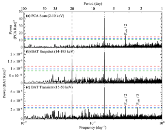
Figure 3.— Semi-weighted power spectra of IGR J16493–4348 using the (a) RXTE PCA scan (2–10 keV), (b) Swift BAT 70-month snapshot (14-195 keV), and (c) Swift BAT transient monitor (15–50 keV) light curves. The horizontal dashed lines indicate 95% (shown in green), 99% (shown in blue), and 99.9% (shown in red) significance levels. The grey vertical dashed line corresponds to the 20.067 day superorbital period from the semi-weighted DFT of the BAT transient monitor data. The 6.7821 day orbital period from the semi-weighted DFT of the BAT transient monitor light curve is indicated by the grey vertical dot-dashed line. Significant harmonics of the orbital period are labeled in each power spectrum.

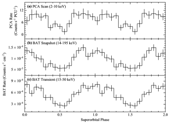
Figure 4.— (a) RXTE PCA scan (2–10 keV), (b) Swift BAT 70-month snapshot (14–195 keV), and (c) Swift BAT transient monitor (15–50 keV) light curves of IGR J16493–4348 folded using 15 bins on the 20.067 day superorbital period measurement from the semi-weighted DFT of the BAT transient monitor data. Superorbital phase 0 corresponds to the time of maximum flux in the BAT transient monitor data (MJD 55329.65647), which was determined from a sine wave fit to the light curve.

Next, we investigated whether there was an energy dependent phase shift between the superorbital modulation detected in the semi-weighted DFTs of the PCA and BAT light curves by cross-correlating the folded, binned light curves against each other using Equation (1), after applying phase offsets to one of the light curves. Linear interpolation was used to determine the count rates of the phase shifted light curve at the phase bins of the unshifted light curve. These linearly interpolated count rates and the count rates from the unshifted light curve were used to compute the cross-correlation statistics. The normalized, linear cross-correlation coefficient between two vectors $\mathbf{u}$ and $\mathbf{v}$ of length $N$ is defined by:

$$r=\mathrm{Re}\frac{\left\langle\mathbf{u,}\mathbf{v}\right\rangle}{\left\|\mathbf{u}\right\|\left\|\mathbf{v}\right\|},$$ (1)

where $\left\|\mathbf{u}\right\|$ and $\left\|\mathbf{v}\right\|$ are the magnitudes of vectors $\mathbf{u}$ and $\mathbf{v}$, and $\mathbf{u}$ and $\mathbf{v}$ are normalized vectors given by $\mathbf{u}=\mathbf{U}-\bar{U}$ and $\mathbf{v}=\mathbf{V}-\bar{V}$, with $\bar{U}$ and $\bar{V}$ denoting the mean of data vectors $\mathbf{U}$ and $\mathbf{V}$, respectively. The inner product between vectors $\mathbf{u}$ and $\mathbf{v}$ is given by:

$$\left\langle\mathbf{u,}\mathbf{v}\right\rangle=\sum_{i=1}^{N}u_{i}v_{i}^{*}$$ (2)

Each pair of light curves was folded on the superorbital period using $N$ $=$ 20, 40, 50, 60, and 80 bins. Phase shifts, in steps of $N^{\text{--1}}$, 0.5$N^{\text{--1}}$, 0.1$N^{\text{--1}}$, and 0.01$N^{\text{--1}}$, were applied to the shifted light curve at each iteration during separate analyses using each of these binnings. A total of 20 analyses were performed for each set of light curves, and the superorbital phase corresponding to the maximum cross-correlation value is given by the average of the superorbital phase bins with maximum cross-correlation values from all 20 analyses.

Uncertainties on these measurements were derived from a total of 2,000,000 Monte Carlo simulations, where 100,000 simulations were performed for each binning and phase shift value. At the beginning of each Monte Carlo iteration, we replaced each count rate in both of the unfolded light curves with a value selected randomly from a Gaussian distribution, whose mean was equal to the measured count rate from the unmodified light curves and standard deviation was given by its associated uncertainty. The resultant light curves were then folded on the superorbital period, binned, and cross-correlated using Equation (1). The error for each set of Monte Carlo analyses was calculated from the standard deviation of the superorbital phase bins with maximum cross-correlation values, and we quote an uncertainty given by the average of all the standard deviations produced by the Monte Carlo procedure.

We find a maximum cross-correlation value between the folded PCA scan and BAT transient monitor light curves at phase 0.02 $\pm$ 0.04 of the superorbital period. We repeated this analysis for the PCA scan and BAT 70-month snapshot light curves, and also pairing the BAT 70-month snapshot and transient monitor light curves, and found that the maximum cross-correlation value occured at superorbital phases –0.02 $\pm$ 0.04 and 0.00 $\pm$ 0.05, respectively. No significantly detected phase offset is observed between the folded PCA and BAT superorbital profiles, which indicates that an energy dependent phase shift is not present.

3.2. Orbital Period

Highly significant peaks were detected in the power spectra shown in Figure 3 at the previously reported 6.8 day orbital period (Corbet et al., 2010a; Cusumano et al., 2010). We measured orbital periods of 6.784 $\pm$ 0.001, 6.788 $\pm$ 0.002, and 6.7821 $\pm$ 0.0008 days from semi-weighted DFTs of the PCA scan, BAT 70-month snapshot, and BAT transient monitor light curves. The FAPs were 3 $\times$ 10${}^{\text{--15}}$, 5 $\times$ 10${}^{\text{--9}}$, and 2 $\times$ 10${}^{\text{--12}}$, respectively. The orbital period was most significantly detected in the power spectrum of the PCA scan light curve, but the BAT transient monitor data yielded the most precise orbital period measurement due to the longer light curve duration. Harmonics of the orbital period were also significantly detected in the power spectra of the PCA scan and BAT transient monitor light curves and are labeled in Figures 3(a) and 3(c).

3.2.1 Observed Minus Calculated Analysis

We carried out an O–C analysis to obtain improved measurements of IGR J16493–4348’s orbital period and orbital period derivative using observed mid-eclipse times from the BAT transient monitor and PCA scan light curves. The BAT light curve was divided into six 638 day time intervals, and the PCA light curve was split into two 1348 day segments. At the beginning of the first iteration, we folded each of these divided light curves on the 6.7821 day orbital period from the semi-weighted DFT of the BAT transient monitor light curve. Each divided BAT light curve was folded on the orbital period using 200 bins. Since the PCA light curves were sampled every $\sim$5 days on average, they were not binned to prevent cycle-to-cycle source brightness variations from affecting the folded orbital profiles.

Eclipses were only visible in the BAT and PCA scan light curves after folding the data on the orbital period. We modeled the eclipses in each folded light curve using asymmetric and symmetric step and ramp functions defined in Equation (3), where the intensities before ingress, during eclipse, and after egress were assumed to remain constant and change linearly during the ingress and egress transitions (Coley et al., 2015). The symmetric model imposes constraints requiring that both the ingress and egress durations and pre-ingress and post-egress count rates be equal. In the asymmetric model, these constraints were removed and the ingress duration, egress duration, and count rates before ingress and after egress were independent free parameters in the model. The adjustable parameters in these models were the: phases corresponding to the start of ingress and start of egress, $\phi_{\text{ing}}$ and $\phi_{\text{egr}}$, ingress duration, $\Delta\phi_{\text{ing}}$, egress duration, $\Delta\phi_{\text{egr}}$, pre-ingress count rate, $C_{\text{ing}}$, post-egress count rate, $C_{\text{egr}}$, and eclipse count rate, $C_{\text{ecl}}$. $C_{\text{ing}}$ was fit from orbital phase $\phi$ $=$ –0.2 to the start of ingress, $C_{\text{ecl}}$ was fit during the eclipse, and $C_{\text{egr}}$ was fit from the end of egress to orbital phase $\phi$ $=$ 0.2. A schematic of the asymmetric eclipse model is shown in Figure 5. The eclipse duration was calculated using Equation (4), and the mid-eclipse phase was found using Equation (5). The eclipse half-angle is defined by Equation (6).

$$C(\phi)=\left\{\begin{array}[]{lc}C_{\text{ing}},&-0.2\leq\phi\leq\phi_{\text{ing}}\\ C_{\text{ing}}+\left(\frac{C_{\text{ecl}}-C_{\text{ing}}}{\Delta\phi_{\text{ing}}}\right)(\phi-\phi_{\text{ing}}),&\phi_{\text{ing}}\leq\phi\leq\phi_{\text{ing}}+\Delta\phi_{\text{ing}}\\ C_{\text{ecl}},&\phi_{\text{ing}}+\Delta\phi_{\text{ing}}\leq\phi\leq\phi_{\text{egr}}\\ C_{\text{ecl}}+\left(\frac{C_{\text{egr}}-C_{\text{ecl}}}{\Delta\phi_{\text{egr}}}\right)(\phi-\phi_{\text{egr}}),&\phi_{\text{egr}}\leq\phi\leq\phi_{\text{egr}}+\Delta\phi_{\text{egr}}\\ C_{\text{egr}},&\phi_{\text{egr}}+\Delta\phi_{\text{egr}}\leq\phi\leq 0.2\end{array}\right.$$ (3)

$$\Delta\phi_{\text{ecl}}=\phi_{\text{egr}}-\left(\phi_{\text{ing}}+\Delta\phi_{\text{ing}}\right)$$ (4)

$$\phi_{\text{mid}}=\frac{1}{2}\left[\phi_{\text{egr}}+\left(\phi_{\text{ing}}+\Delta\phi_{\text{ing}}\right)\right]$$ (5)

$$\Theta_{e}=\Delta\phi_{\text{ecl}}\times 180^{\circ}$$ (6)

Flares were excluded when fitting the eclipse models to the folded PCA scan light curves, which were identified by data points with count rates above 20 counts s${}^{\text{--1}}$ PCU${}^{\text{--1}}$ at orbital phases near the start of ingress or end of egress. This resulted in the removal of approximately 6% of the data from the fitted PCA scan light curves. We chose to remove these data points with high count rates since they increased the fitted $\chi^{\mathrm{2}}$ values, but did not significantly affect the best-fit parameters or their uncertainties.

Observed mid-eclipse times from each folded light curve were determined using Equation (5). We fit the observed mid-eclipse times using the orbital change function:

$$T_{n}=T_{\pi/2}+nP_{\text{orb}}+\frac{1}{2}n^{2}P_{\text{orb}}\dot{P}_{\text{orb}},$$ (7)

where $T_{n}$ is the mid-eclipse time in days, $n$ is the nearest integer number of elapsed binary orbits, $P_{\text{orb}}$ is the orbital period in days, and $\dot{P}_{\text{orb}}$ is the orbital period derivative at $T_{\pi/2}$. Each mid-eclipse time was weighted by its maximum asymmetric error in Table 2 during the fitting procedure. After each iteration, the orbital period and $T_{\pi/2}$ were updated with the values obtained from fitting the mid-eclipse times with the orbital change function in Equation (7), and these values were used to refold the BAT and PCA light curves in the next iteration. The O–C procedure was repeated until there were no significant changes in the orbital period and $T_{\pi/2}$ between successive iterations.

We observed that many of the parameters in these models were highly covariant from projections of their posterior distributions. A Bayesian MCMC fitting procedure was used to incorporate these covariances into the model parameter uncertainties by marginalizing over multi-dimensional joint posterior distributions. From Bayes’ theorem, the posterior probability of a set of model parameters, $\bm{\theta}$, given the observed data, $\bm{D}$, and any prior information, $\bm{I}$, is defined by:

$$p(\bm{\theta}|\bm{D},\bm{I})=\frac{p(\bm{D}|\bm{\theta},\bm{I})p(\bm{\theta}|\bm{I})}{p(\bm{D}|\bm{I})}$$ (8)

Here, $p(\bm{D}|\bm{\theta},\bm{I})=\mathcal{L}(\bm{\theta}|\bm{D},\bm{I})$ is the likelihood function, $p(\bm{\theta}|\bm{I})=\pi(\bm{\theta}|\bm{I})$ is the prior probability distribution for the model parameters, and $p(\bm{D}|\bm{I})$ is the marginal likelihood function. The marginal likelihood function can be thought of as a normalization constant, determined by requiring the posterior probability integrate to unity when integrating over all of the parameters in the model. Marginalized single parameter posterior distributions were obtained by integrating the joint posterior distribution over the remaining parameters:

$$p(\theta_{i}|\bm{D},\bm{I})\propto\int_{\mathcal{V}}d^{n}\bm{\theta^{\prime}}\mathcal{L}(\bm{\theta}|\bm{D},\bm{I})\pi(\bm{\theta}|\bm{I}),$$ (9)

where $\bm{\theta^{\prime}}$ is a parameter vector equal to $\bm{\theta}$ excluding $\theta_{i}$ and $\mathcal{V}$ is the integration volume of the parameter space. We assumed uninformed, flat priors on all of our model parameters and used a Gaussian likelihood function, such that $\mathcal{L}(\bm{\theta}|\bm{D},\bm{I})\propto\text{exp}(-\chi^{2}/2)$.

An affine-invariant MCMC ensemble sampler (Goodman & Weare, 2010), implemented in emcee by Foreman-Mackey et al. (2013), was used to sample the posterior probability density functions (PDFs) of the model parameters in Equations (3) and (7). The parameter spaces were explored using 200 walkers and a chain length of 1,500 steps per walker. The first 500 steps in each chain were treated as the initial burn-in phase and were removed from the analysis. The position of each walker was updated using the current positions of all of the other walkers in the ensemble (Goodman & Weare, 2010). We initialized the walkers to start from a small Gaussian ball centered around the parameter values obtained from maximizing the likelihood function subject to the constraints given by the priors. The posterior distributions of the model parameters were calculated using the remaining 1,000 steps in each chain. Best-fit values for the model parameters were derived from the median of the marginalized posterior distributions, and we quote 1$\sigma$ uncertainties using Bayesian credible intervals.

In Table 2, we list the observed mid-eclipse times obtained from the O–C analysis using asymmetric and symmetric eclipse models. These measurements are also plotted in the top panels of Figures 6 and 6, along with the best-fit orbital change functions. The residuals were derived by subtracting the fits from the mid-eclipse times and are shown in the bottom panels of these figures. We note that our mid-eclipse times are consistent with the mid-eclipse time reported by Cusumano et al. (2010) using Swift BAT survey (15–50 keV) data, which we indicate with blue triangles in these plots.

We refine the orbital period to 6.7828 $\pm$ 0.0004 days using an asymmetric eclipse model and a fiducial mid-eclipse time of $T_{\pi/2}$ $=$ MJD 55851.3 $\pm$ 0.1 in our O–C analysis. A consistent orbital period of 6.7825 $\pm$ 0.0004 days was found using a symmetric eclipse model with $T_{\pi/2}$ $=$ MJD 55851.21 $\pm$ 0.07. Orbital period derivatives of 0.01${}^{\text{+1.74}}_{\text{--1.77}}$ $\times$ 10${}^{\text{--7}}$ d d${}^{\text{--1}}$ and 0.09${}^{\text{+1.69}}_{\text{--1.73}}$ $\times$ 10${}^{\text{--7}}$ d d${}^{\text{--1}}$ were measured by fitting the asymmetric and symmetric mid-eclipse times with the orbital change function in Equation (7), respectively. These values indicate that there was no significant change in the orbital period over approximately 500 orbital cycles.

We selected the period obtained from using an asymmetric eclipse model in the O–C analysis as our preferred orbital period measurement. Since most eclipsing sgHMXBs show evidence of asymmetry in their X-ray eclipses (e.g., Falanga et al. 2015), we argue that an asymmetric eclipse model is more representative of the eclipse behavior in these systems. Additionally, constraints on the eclipse transition durations and count rates outside of the eclipses could introduce systematic errors when fitting the folded light curves with a symmetric eclipse model.

Figure 5.— Schematic of the asymmetric step and ramp function in Equation (3), which was used to model the eclipses in the folded RXTE PCA scan (2–10 keV), Swift BAT 70-month snapshot (14–195 keV), and Swift BAT transient monitor (15–50 keV) light curves.

Table 2Mid-Eclipse Times of IGR J16493–4348 from O–C Analysis

Observation	Orbital Cycle	Mid-Eclipse Timea	Mid-Eclipse Timeb
	($n$)	(MJD)	(MJD)
BAT Transient Monitor	–312	53735.2${}^{\text{+0.2}}_{\text{--0.1}}$	53735.2 $\pm$ 0.1
PCA Scan	–297	53836.69${}^{\text{+0.09}}_{\text{--0.08}}$	53836.76${}^{\text{+0.09}}_{\text{--0.07}}$
BAT Transient Monitor	–217	54379.5 $\pm$ 0.2	54379.4 $\pm$ 0.2
BAT Transient Monitor	–124	55010.4${}^{\text{+0.4}}_{\text{--0.3}}$	55010.3 $\pm$ 0.3
PCA Scan	–98	55186.51${}^{\text{+0.10}}_{\text{--0.09}}$	55186.52 $\pm$ 0.06
BAT Transient Monitor	–29	55654.7${}^{\text{+0.2}}_{\text{--0.3}}$	55654.7 $\pm$ 0.3
BAT Transient Monitor	65	56292.2${}^{\text{+0.4}}_{\text{--0.2}}$	56292.1 $\pm$ 0.3
BAT Transient Monitor	159	56929.7${}^{\text{+0.3}}_{\text{--0.2}}$	56929.6${}^{\text{+0.3}}_{\text{--0.2}}$

Note. — We quote 1$\sigma$ uncertainties using Bayesian credible intervals.

^a Obtained using an asymmetric eclipse model.

^b Obtained using a symmetric eclipse model.

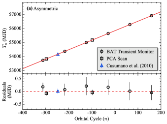
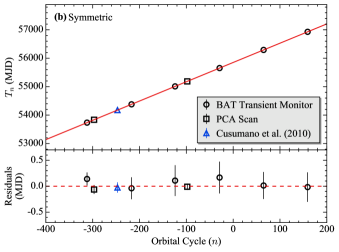
Figure 6.— Top panels: Observed mid-eclipse times of IGR J16493–4348 obtained from an O–C analysis using the RXTE PCA scan (2–10 keV) and Swift BAT transient monitor (15–50 keV) light curves and (a) asymmetric and (b) symmetric eclipse models. The solid red line corresponds to the best-fit orbital change function using Equation (7). Each mid-eclipse time was weighted by its maximum asymmetric error in Table 2 during the fitting procedure. Bottom panels: Residuals determined by subtracting the best fit from the mid-eclipse times. Mid-eclipse times derived from the BAT transient monitor and PCA scan light curves are represented by black open circles and black open squares, respectively. The mid-eclipse time measurement reported by Cusumano et al. (2010) is indicated with blue open triangles.

3.2.2 Folded Orbital Profiles

Orbital profiles were produced by folding the PCA scan, BAT 70-month snapshot, and BAT transient monitor light curves on the orbital periods from the O–C analysis in Section 3.2.1. Asymmetric and symmetric eclipse models, defined in Equation (3), were fit to each of the folded light curves using the Bayesian MCMC procedure described in Section 3.2.1 with the same number of walkers and chain lengths. In Tables 3 and 4, we list the best-fit eclipse model parameters from the median of the marginalized posterior distributions, along with 1$\sigma$ uncertainties using Bayesian credible intervals. The folded orbital profiles are shown in Figures 7(a)–(c), and the best-fit asymmetric and symmetric eclipse models are overlaid in green and red, respectively.

The mid-eclipse times ($T_{\text{mid}}$), calculated in Tables 3 and 4 using Equation (5), are consistent with each other at the 1$\sigma$ level. Fitting an asymmetric eclipse model to the folded PCA scan, BAT 70-month snapshot, and BAT transient monitor light curves yielded eclipse durations of 0.9 $\pm$ 0.1, 0.7${}^{\text{+0.2}}_{\text{--0.3}}$, and 0.7 $\pm$ 0.3 days, respectively. Using a symmetric eclipse model, we measured eclipse lengths of 0.92${}^{\text{+0.10}}_{\text{--0.09}}$, 0.8 $\pm$ 0.2, and 0.8 $\pm$ 0.2 days, respectively. These eclipse durations are all consistent with each other to within 1$\sigma$ and agree well with the $\sim$0.8 day eclipse length reported by Cusumano et al. (2010) from BAT survey observations. There were no statistically significant differences between the ingress and egress durations or pre-ingress and post-egress count rates obtained from fitting the light curves with an asymmetric eclipse model. This suggests that large-scale structure in the stellar wind from a strong accretion or photoionization wake is unlikely.

Table 3Asymmetric Eclipse Model Parameters of IGR J16493–4348

Model Parameter	RXTE PCA	Swift BAT	Swift BAT
	Galactic Bulge Scans	70-month Snapshots	Transient Monitor
	(2–10 keV)	(14–195 keV)	(15–50 keV)
$\phi_{\text{ing}}$	–0.092${}^{\text{+0.005}}_{\text{--0.007}}$	–0.10${}^{\text{+0.02}}_{\text{--0.01}}$	–0.12${}^{\text{+0.01}}_{\text{--0.02}}$
$\phi_{\text{egr}}$	0.059${}^{\text{+0.009}}_{\text{--0.011}}$	0.06${}^{\text{+0.02}}_{\text{--0.03}}$	0.05${}^{\text{+0.01}}_{\text{--0.03}}$
$\Delta\phi_{\text{ing}}$	0.023${}^{\text{+0.011}}_{\text{--0.009}}$	0.05${}^{\text{+0.03}}_{\text{--0.02}}$	0.06${}^{\text{+0.05}}_{\text{--0.03}}$
$\Delta\phi_{\text{egr}}$	0.06${}^{\text{+0.04}}_{\text{--0.03}}$	0.07${}^{\text{+0.05}}_{\text{--0.04}}$	0.09 $\pm$ 0.04
$C_{\text{ing}}$	7.5 $\pm$ 0.8a	0.11 $\pm$ 0.01b	0.63 $\pm$ 0.07b
$C_{\text{egr}}$	6.7 $\pm$ 1.1a	0.09${}^{\text{+0.02}}_{\text{--0.01}}$b	0.64${}^{\text{+0.10}}_{\text{--0.08}}$b
$C_{\text{ecl}}$	–3.5 $\pm$ 0.6a	–0.001${}^{\text{+0.013}}_{\text{--0.014}}$b	–0.03${}^{\text{+0.06}}_{\text{--0.07}}$b
$\Delta\phi_{\text{ecl}}$	0.13${}^{\text{+0.01}}_{\text{--0.02}}$	0.11 $\pm$ 0.04	0.11${}^{\text{+0.05}}_{\text{--0.04}}$
$P_{\text{orb}}$c	6.7828 $\pm$ 0.0004	6.7828 $\pm$ 0.0004	6.7828 $\pm$ 0.0004
$\dot{P}_{\text{orb}}$d	0.01${}^{\text{+1.74}}_{\text{--1.77}}$	0.01${}^{\text{+1.74}}_{\text{--1.77}}$	0.01${}^{\text{+1.74}}_{\text{--1.77}}$
$T_{\text{mid}}$e	55851.2 $\pm$ 0.1	55851.3 $\pm$ 0.2	55851.2 $\pm$ 0.2
$\Theta_{e}$f	22.9${}^{\text{+2.7}}_{\text{--2.8}}$	19.0${}^{\text{+6.4}}_{\text{--7.9}}$	19.5${}^{\text{+9.2}}_{\text{--7.3}}$
$\chi_{\nu}^{\mathrm{2}}$ (dof)	1.22 (197)	1.10 (73)	1.16 (73)

Note. — We quote 1$\sigma$ uncertainties using Bayesian credible intervals. Phase 0 is defined at mid-eclipse.

^a Units are counts s${}^{\text{--1}}$ PCU${}^{\text{--1}}$.

^b Units are 10${}^{\text{--3}}$ counts cm${}^{\text{--2}}$ s${}^{\text{--1}}$.

^c Refined orbital period from O–C analysis. Units are days.

^d Orbital period derivative from orbital change function. Units are 10${}^{\text{--7}}$ d d${}^{\text{--1}}$.

^e Units are MJD.

^f Units are degrees.

Table 4Symmetric Eclipse Model Parameters of IGR J16493–4348

Model Parameter	RXTE PCA	Swift BAT	Swift BAT
	Galactic Bulge Scans	70-month Snapshots	Transient Monitor
	(2–10 keV)	(14–195 keV)	(15–50 keV)
$\phi_{\text{ing}}$	–0.100${}^{\text{+0.006}}_{\text{--0.008}}$	–0.10${}^{\text{+0.02}}_{\text{--0.01}}$	–0.12 $\pm$ 0.01
$\phi_{\text{egr}}$	0.064 $\pm$ 0.006	0.06${}^{\text{+0.02}}_{\text{--0.01}}$	0.06 $\pm$ 0.01
$\Delta\phi$a	0.03 $\pm$ 0.01	0.05${}^{\text{+0.02}}_{\text{--0.03}}$	0.06${}^{\text{+0.03}}_{\text{--0.02}}$
$C$b	6.9 $\pm$ 0.5c	0.105${}^{\text{+0.010}}_{\text{--0.009}}$d	0.62 $\pm$ 0.05d
$C_{\text{ecl}}$	–3.6 $\pm$ 0.6c	0.002${}^{\text{+0.012}}_{\text{--0.013}}$d	–0.03 $\pm$ 0.06d
$\Delta\phi_{\text{ecl}}$	0.14${}^{\text{+0.02}}_{\text{--0.01}}$	0.11${}^{\text{+0.04}}_{\text{--0.03}}$	0.11 $\pm$ 0.03
$P_{\text{orb}}$e	6.7825 $\pm$ 0.0004	6.7825 $\pm$ 0.0004	6.7825 $\pm$ 0.0004
$\dot{P}_{\text{orb}}$f	0.09${}^{\text{+1.69}}_{\text{--1.73}}$	0.09${}^{\text{+1.69}}_{\text{--1.73}}$	0.09${}^{\text{+1.69}}_{\text{--1.73}}$
$T_{\text{mid}}$g	55851.19 $\pm$ 0.09	55851.3 $\pm$ 0.1	55851.2 $\pm$ 0.1
$\Theta_{e}$h	24.5${}^{\text{+2.8}}_{\text{--2.5}}$	20.0${}^{\text{+6.6}}_{\text{--6.2}}$	19.9${}^{\text{+6.1}}_{\text{--5.2}}$
$\chi_{\nu}^{\mathrm{2}}$ (dof)	1.17 (198)	1.25 (75)	0.97 (75)

Note. — We quote 1$\sigma$ uncertainties using Bayesian credible intervals. Phase 0 is defined at mid-eclipse.

^a $\Delta\phi=\Delta\phi_{\text{ing}}=\Delta\phi_{\text{egr}}$, assuming equal ingress and egress durations.

^b $C=C_{\text{ing}}=C_{\text{egr}}$, assuming equal pre-ingress and post-egress count rates.

^c Units are counts s${}^{\text{--1}}$ PCU${}^{\text{--1}}$.

^d Units are 10${}^{\text{--3}}$ counts cm${}^{\text{--2}}$ s${}^{\text{--1}}$.

^e Orbital period from O–C analysis. Units are days.

^f Orbital period derivative from orbital change function. Units are 10${}^{\text{--7}}$ d d${}^{\text{--1}}$.

^g Units are MJD.

^h Units are degrees.

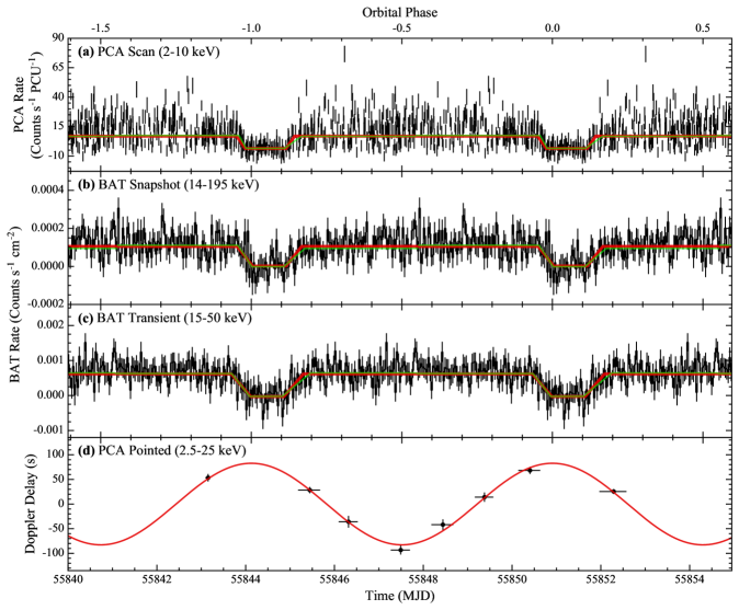
Figure 7.— (a) RXTE PCA scan (2–10 keV), (b) Swift BAT 70-month snapshot (14–195 keV), and (c) Swift BAT transient monitor (15–50 keV) light curves of IGR J16493–4348 folded on the refined 6.7828 day orbital period from the O–C analysis in Section 3.2.1. The BAT light curves were folded using 200 bins. The PCA scan light curve was not binned to prevent cycle-to-cycle source brightness variations from affecting the folded orbital profile. We overlay the asymmetric (shown in green) and symmetric (shown in red) step and ramp eclipse models from Tables 3 and 4. Discontinuities in the asymmetric eclipse model are included at half orbital cycles from the mid-eclipse times. (d) Orbital Doppler delay times measured during the final iteration of the pulsar timing analysis using the pointed RXTE PCA (2.5–25 keV) light curve of IGR J16493–4348. The uncertainties on the ToAs correspond to the statistical errors obtained from Monte Carlo simulations and do not include the additional 3.1 s systematic uncertainty from circular solution 2 in Table 6. The horizontal error bars indicate the duration of the light curve segments used to derive the ToAs. The red curve shows the predicted delay times using the fit from circular solution 1 in Table 6, which assumes a constant neutron star rotational period. Orbital phase 0 corresponds to $T_{\pi/2}$ from circular solution 1 in Table 6.

3.3. Pulse Period

We searched for pulsations with periods between 32 s and 9.5 days in the unweighted power spectrum of the entire pointed RXTE PCA (2.5–25 keV) light curve. The power spectrum was oversampled by a factor of five compared to the nominal frequency resolution, which was found to be 1.22 $\times$ 10${}^{\text{--6}}$ Hz from the length of the light curve. The data in the pointed PCA power spectrum were not weighted since the observations were performed using the same pointing and the light curve had a uniform time resolution of 16 s.

A significant amount of low frequency noise was detected in the power spectrum shown in Figure 8(a). We estimated the continuum noise level by fitting polynomials to the logarithm of the power spectrum in Figure 8(b) after adding a constant value of 0.25068 to remove the bias from the $\chi^{\mathrm{2}}$ distribution of the log-spectrum (Papadakis & Lawrence, 1993; Vaughan, 2005). We found that fitting a linear function to the log-spectrum, which would indicate a power law relationship in the raw power spectrum, was not optimal for describing the power at low frequencies. A quadratic fit significantly overestimated the low frequency power, and we found that a cubic fit to the log-spectrum sufficiently characterized the continuum noise level. The red noise was removed by subtracting the cubic fit from the logarithm of the power spectrum, which produced the corrected power spectrum in Figure 8(c). We find strong evidence of pulsed emission at a period of 1093.3 $\pm$ 0.1 s in the corrected power spectrum, which we associate with the rotational period of the neutron star. This pulse period is labeled by the vertical dot-dashed line in Figure 8.

At lower frequencies, there are significant peaks near the $\sim$5800 s orbital period of RXTE, which exhibit complex structure. The 95%, 99%, and 99.9% significance levels are labeled in Figure 8(c), but do not account for the uncertainty in the model used to fit the continuum or the red noise subtraction. These effects are greatest at low frequencies, and larger power levels would be required to achieve these true levels of statistical significance. We also note that none of the low frequency peaks in the uncorrected power spectrum are statistically significant after the continuum noise was removed.

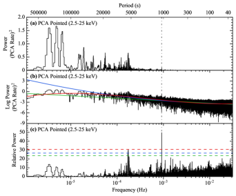
Figure 8.— (a) Unweighted power spectrum of IGR J16493–4348 using the pointed RXTE PCA (2.5–25 keV) light curve without low frequency noise subtracted from the continuum. (b) Linear (shown in green), quadratic (shown in blue), and cubic (shown in red) fits to the logarithm of the power spectrum. The cubic fit was used to estimate and remove the continuum noise. (c) Corrected power spectrum after subtracting the cubic continuum noise model. The horizontal dashed lines indicate the 95% (shown in green), 99% (shown in blue), and 99.9% (shown in red) significance levels. The vertical dot-dashed line corresponds to the 1093 s pulse period. The statistically significant peaks near $\sim$5800 s are attributed to the orbital period of RXTE.

4. System Geometry

A pulsar timing algorithm was developed to accurately measure the neutron star rotational period and orbital parameters of IGR J16493–4348 by fitting circular and eccentric orbital timing models to the ToAs. These results are presented here, along with a rigorous treatment of the statistical and systematic uncertainties associated with the ToAs. We also provide measurements of additional parameters constraining the system geometry, such as the eclipse half-angle, donor star spectral type, and Roche lobe radius, for different possible inclinations and neutron star masses.

4.1. Pulsar Timing Analysis

We carried out a phase-coherent pulsar timing analysis using the pointed RXTE PCA (2.5–25 keV) light curve, where each rotation of the pulsar was unambiguously accounted for over the time span of the observations. An iterative epoch folding algorithm (Leahy et al., 1983; Schwarzenberg-Czerny, 1989; Chakrabarty, 1996) was used to derive the ToAs. Epoch folding is useful because of its higher sensitivity to non-sinusoidal pulse shapes and ability to handle gaps in the light curve. The ToAs were obtained by measuring phase offsets between a pulse template and individual measured profiles, which were created by dividing the light curve into smaller segments.

The measured profiles were created by first dividing the pointed PCA light curve into individual segments spanning at least one pulse period in duration. Data within 20 ks of another segment were merged together. Neighboring segments were separated by at least 36 ks, and the segment durations ranged from 8.4 to 52.8 ks. This produced a total of eight segments from which ToAs were derived. We partitioned the data in this manner to optimize both the signal-to-noise of the pulsations in each segment and the final number of ToAs.

An initial set of measured profiles were produced by folding each segment on the 1093.3 s pulse period found in the noise subtracted power spectrum of the pointed PCA light curve (see Section 3.3). The segments were folded using 68 bins, which provided a time resolution equal to the 16 s sampling rate in the light curve. A preliminary pulse template was created by aligning the measured profiles and averaging the count rates in each bin. The uncertainties on the count rates in the pulse template were calculated by summing the errors in each bin in quadrature and then normalizing by the total number of measured profiles. This method of generating an initial template is beneficial because it incorporates the effects of the binary system’s orbital motion, which are neglected when the entire light curve is folded on the pulse period.

Next, the phase offset between the pulse template and each of the measured profiles was determined by cross-correlating the two profiles in the Fourier frequency domain (Taylor, 1992). It is advantageous to calculate the cross-correlation in the frequency domain, as opposed to using time-domain techniques, because it circumvents systematic errors due to binning and allows for the ToAs to be measured with greater accuracy. Assuming that the measured profile is a scaled and shifted version of the pulse template, a phase shift is equivalent to multiplying the template by a complex exponential. The phase shift between each measured profile, $d(\phi)$, and the pulse template, $p(\phi)$, was found by minimizing (Taylor, 1992; Koh et al., 1997; Demorest, 2007):

$$\chi^{2}(A,\phi)=\sum_{k=1}^{k_{\text{max}}}\frac{\left|d_{k}-Ap_{k}e^{-2\pi ik\phi}\right|^{2}}{\sigma_{k}^{2}},$$ (10)

where $d_{k}=\sum_{j}d(j/N)e^{-2\pi ijk/N}$ is the DFT of $d(\phi)$, $p_{k}=\sum_{j}p(j/N)e^{-2\pi ijk/N}$ is the DFT of $p(\phi)$, $\sigma_{k}^{2}$ is the noise power at each frequency bin of the DFT, and $A$ and $\phi$ are the measured amplitude and phase shift, respectively.

Several of the observations did not exhibit strong pulsed emission (see the bold entries in Table 1) and were excluded from the pulsar timing analysis since their measured profiles yielded phase offsets that could not be well constrained during the cross-correlation procedure. The omitted data spanned MJDs 55843.87475 to 55844.56803 (orbital phases –0.037 to 0.065) and MJDs 55851.18401 to 55851.48269 (orbital phases 0.041 to 0.085), where orbital phase 0 is defined at $T_{\pi/2}$ from circular solution 1 in Table 6. The excised data are shown in red in Figure 1 and coincide with the eclipse and eclipse transition phases measured from fitting the folded PCA and BAT orbital profiles with asymmetric and symmetric eclipse models (see Section 3.2.2).

Pulse time delays were obtained by multiplying the phase differences between each of the measured profiles and the pulse template by the folding period. The ToAs were derived by adding each time delay to the time nearest to the middle of its corresponding observation interval where the pulsar rotational phase was zero. Referencing each ToA relative to the middle of the interval reduces systematic effects that can arise from folding with an inaccurate timing model and is a standard convention used in pulsar timing (e.g., Levine et al. 2004).

Folding the data with a slightly incorrect pulse period can lead to pulse smearing and produce ToAs that show a drift in pulse phase over the observation duration. At the end of each iteration, a small correction was applied to the pulse period using the drift rate measured from the ToAs. This improved pulse period measurement was then used to refold each of the segments to produce corrected measured profiles and a sharper pulse template in the following iteration. A refined pulse template was constructed by averaging the corrected measured profiles together without any alignment, and a new set of ToAs was produced by cross-correlating the measured profiles with the updated pulse template in the frequency domain. This algorithm was repeated until there was no statistically significant change in the pulse period between successive iterations.

We refine the pulse period to 1093.1036 $\pm$ 0.0004 s using the ToAs obtained during the last iteration of the pulsar timing analysis. The final pulse template (2.5–25 keV), shown in Figure 9, exhibits sharp features on top of a quasi-sinusoidal template shape. These sharp variations in the pulse template enabled the phase shifts between the measured profiles and the template to be determined more accurately. A list of ToAs measured during the final iteration of the pulsar timing analysis is provided in Table 5. Pulse profiles in the 2.5–5, 5–10, 10–25, and 2.5–25 keV energy bands are shown in Figure 10 and were obtained by folding the pointed PCA light curves on the final pulse period measurement after correcting for orbital Doppler delays. We define the peak-to-peak pulsed fraction as:

$$\mathcal{P}=\frac{(F_{\text{max}}-F_{\text{min}})}{(F_{\text{max}}+F_{\text{min}})},$$ (11)

where $F_{\text{max}}$ and $F_{\text{min}}$ are the maximum and minimum count rates in the pulse profile, respectively. Using Equation (11), the pulsed fractions in the 2.5–5, 5–10, 10-25, and 2.5–25 keV energy bands are 0.08 $\pm$ 0.02, 0.12 $\pm$ 0.02, 0.27 $\pm$ 0.04, and 0.13 $\pm$ 0.02, respectively. These measurements indicate an increase in pulsed fraction with increasing X-ray energy.

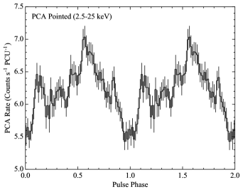
Figure 9.— Final pulse template of IGR J16493–4348 obtained during the last iteration of the pulsar timing analysis using the pointed RXTE PCA (2.5–25 keV) light curve. The count rates in each bin were derived by averaging the count rates in the measured profiles. The uncertainties were calculated by summing the errors on the count rates in each bin of the measured profiles in quadrature and then normalizing by the total number of profiles. Phase 0 corresponds to $T_{\pi/2}$ from circular solution 1 in Table 6.

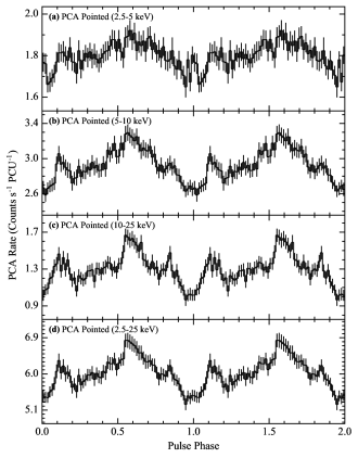
Figure 10.— Pulse profiles of IGR J16493–4348 derived from pointed RXTE PCA observations in the (a) 2.5–5, (b) 5–10, (c) 10–25, and (d) 2.5–25 keV energy bands. The profiles were obtained by folding the light curves on the refined 1093 s pulse period measurement from the final iteration of the pulsar timing analysis after correcting for orbital Doppler delays. Phase 0 corresponds to $T_{\pi/2}$ from circular solution 1 in Table 6.

Table 5Pulse Times of Arrival from IGR J16493–4348

ToA	Pulse Cyclea	Statistical Uncertaintyb	Total Uncertaintyc	Pulse Phased
($t_{n}$, MJD)	$(n)$	(s)	(s)
55843.15499	5	7.7	8.3	0.09
55845.44465	186	6.4	7.1	0.07
55846.31687	255	11.9	12.3	0.01
55847.49281	348	9.1	9.6	0.96
55848.44228	423	10.7	11.2	0.01
55849.37915	497	9.4	9.9	0.06
55850.40456	578	7.2	7.9	0.11
55852.28917	727	5.0	5.8	0.07

Note. —

^a Nearest integer pulse cycle calculated using Equation (14) and $t_{0}$ $=$ MJD 55843.09111. Pulse cycles are referenced with respect to the start of the pointed PCA observations.

^b 1$\sigma$ statistical uncertainties derived from Monte Carlo simulations.

^c Total uncertainties calculated by adding a systematic uncertainty of 3.1 s from circular solution 2 in Table 6 to each statistical uncertainty in quadrature.

^d Phase 0 corresponds to $T_{\pi/2}$ from circular solution 1 in Table 6.

4.2. Pulse Time of Arrival Uncertainties

Statistical uncertainties on the ToAs were calculated using 100,000 Monte Carlo simulations (Thompson et al., 2006, 2007). At the beginning of each simulation, the pointed PCA light curve was divided into individual segments according to the procedure described in Section 4.1. Each count rate in the segments was replaced with a value selected randomly from a Gaussian distribution, with mean equal to the original background-subtracted count rate and standard devation given by its associated uncertainty. Simulated measured profiles were produced by folding these randomly generated segments on the refined 1093 s pulse period measurement from the final iteration of the pulsar timing analysis. During each simulation, phase offsets were measured by cross-correlating each of the simulated measured profiles with the final pulse template in the frequency domain, which were then used to derive an independent set of ToAs. We quote 1$\sigma$ statistical uncertainties on each ToA listed in Table 5 from the median absolute deviation of the distribution of simulated ToAs obtained for each segment. The median absolute deviation is a robust statistic that is more resilient to outliers than the standard deviation. We used this statistic to reduce the effect that tails in the distribution of the simulated ToAs had on the statistical errors. The statistical uncertainties ranged from 5.0 to 11.9 s.

Systematic errors in the ToAs can arise from changes in the average pulse profile due to varying flux levels, absorption along the line of sight, or contamination from nearby sources (e.g., Thompson et al. 2006). We modeled the systematic error as a nuisance parameter when fitting the ToAs with timing models using the Bayesian MCMC procedure described in Section 3.2.1. The systematic uncertainty was treated as an additional error that was added in quadrature with the statistical uncertainty in the likelihood function. We marginalized over this systematic uncertainty when constructing posterior PDFs for the model parameters. Due to the limited number of ToAs and few degrees of freedom in the timing solutions, a systematic error was derived only for circular solution 2, which used the same timing model as in circular solution 1 (see Section 4.3 and Table 6). We find a systematic uncertainty of $\sigma_{\text{sys}}$ $=$ 3.1${}^{\text{+3.0}}_{\text{--2.3}}$ s from the median of the marginalized posterior distribution, and we report 1$\sigma$ errors on this measurement using Bayesian credible intervals. This systematic uncertainty was added in quadrature with the statistical uncertainty for each ToA, which yielded the total uncertainties listed in Table 5. We note that the inclusion of systematic errors as a nuisance parameter increased the reduced $\chi^{2}_{\nu}$ value from 0.88 in circular solution 1 to 1.04 in circular solution 2 without significantly affecting the best-fit orbital parameters.

4.3. Pulsar Timing Models

Assuming the pulsar phase varies smoothly as a function of time, a Taylor expansion can be used to approximate the pulse phase, $\phi$, at time $t$:

$$\phi(t)=\phi(t_{0})+\nu_{\text{pulse}}(t-t_{0})+\frac{1}{2}\dot{\nu}_{\text{pulse}}(t-t_{0})^{2}+\cdots,$$ (12)

where $\nu_{\text{pulse}}$ and $\dot{\nu}_{\text{pulse}}$ are the neutron star rotational frequency and its time derivative at a reference time $t_{0}$, typically chosen to be the start time of the observation. Equation (12) can be transformed to give the expected arrival time, $t_{n}^{\prime}$, of the $n$th pulse:

$$t_{n}^{\prime}=t_{0}+nP_{\text{pulse}}+\frac{1}{2}n^{2}P_{\text{pulse}}\dot{P}_{\text{pulse}}+\cdots,$$ (13)

where $P_{\text{pulse}}$ $=$ $\nu_{\text{pulse}}^{-1}$ is the pulse period at time $t_{0}$ and $\dot{P}_{\text{pulse}}$ is the pulse period derivative. The pulse cycle, $n$, associated with each ToA is calculated to the nearest integer using:

$$n=\frac{t_{n}^{\prime}-t_{0}}{P_{\text{pulse}}}-\frac{1}{2}\frac{\dot{P}_{\text{pulse}}}{P_{\text{pulse}}^{2}}(t_{n}^{\prime}-t_{0})^{2}$$ (14)

Additional time delays are observed from binary pulsars due to their orbital motion. In these systems, the ToAs can be described by:

$$t_{n}=t_{n}^{\prime}+f_{\text{orb}}(t_{n}^{\prime}),$$ (15)

where $f_{\text{orb}}(t_{n}^{\prime})$ is the orbital Doppler delay time associated with $t_{n}^{\prime}$. For binary pulsars in circular orbits, the orbital Doppler delay times are given by (Blandford & Teukolsky, 1976; Kelley et al., 1980):

$$f_{\text{orb}}(t_{n}^{\prime})=a_{x}\sin i\cos\left[\frac{2\pi(t_{n}^{\prime}-T_{\pi/2})}{P_{\text{orb}}}\right],$$ (16)

where $a_{x}\sin i$ is the projected semi-major axis of the orbit, $i$ is the orbital inclination angle relative to the line of sight, and $T_{\pi/2}$ is the time of maximum delay and mid-eclipse. If the orbit is eccentric, the Doppler delay times are instead given by (Blandford & Teukolsky, 1976):

where $e$ is the eccentricity, $\omega$ is the longitude of periastron, and $E$ is the eccentric anomaly. The eccentric anomaly can be related to the mean anomaly, $M$, using Kepler’s equation:

$$M=E-e\sin E=\frac{2\pi(t_{n}^{\prime}-T_{\text{peri}})}{P_{\text{orb}}},$$ (18)

where $T_{\text{peri}}$ is the time of periastron passage.

The pulse period behavior and orbital parameters were measured by fitting circular and eccentric orbital timing models to the ToAs in Table 5. The timing models were constructed using Equations (13) and (15), together with Equation (16) for the circular solutions and Equation (17) for the eccentric solutions. To properly account for covariances between the model parameters in the orbital solutions, we used the Bayesian MCMC fitting procedure described in Section 3.2.1.

Circular solutions 1 and 2 and eccentric solution 1 were fit assuming a constant neutron star rotational period. Pulse period changes were incorporated into the timing models used to derive circular solution 3 and eccentric solution 2. In all of these models, the orbital period was fixed to the refined 6.7828 day measurement from the O–C analysis in Section 3.2.1, and the ToAs were weighted by their corresponding uncertainties during the fitting process.

In Table 6, we list the best-fit pulse period and orbital parameter measurements for each timing model, along with 1$\sigma$ uncertainties derived from Bayesian credible intervals. Circular solution 1 is our favored orbital timing model since the fit yielded an acceptable reduced $\chi^{2}_{\nu}$ value with the greatest number of degrees of freedom compared to the other timing models in Table 6. The orbital Doppler delay times measured during the final iteration of the pulsar timing analysis are shown in Figure 7(d), along with the predicted delay times from circular solution 1. We find a projected semi-major axis of $a_{x}\sin i$ $=$ 82.8${}^{\text{+5.0}}_{\text{--5.2}}$ lt-s and a mid-eclipse time of $T_{\pi/2}$ $=$ MJD 55850.91 $\pm$ 0.05 from the fit in circular solution 1. A pulse period derivative of $\dot{P}_{\text{pulse}}$ $=$ –5.4${}^{\text{\text{+7.9}}}_{\text{\text{--9.7}}}$ $\times$ 10${}^{\text{--8}}$ s s${}^{\text{--1}}$ was obtained in circular solution 3, which indicates that there was no statistically significant long-term change in the pulse period during the pointed PCA observations. In addition, no rapid spin-up or spin-down episodes were observed, which suggests that a transient accretion disk is not present in this system (Koh et al., 1997; Jenke et al., 2012).

The X-ray mass function is given by:

$$f_{x}(M)=\frac{4\pi^{2}(a_{x}\sin i)^{3}}{GP_{\text{orb}}^{2}}=\frac{(M_{c}\sin i)^{3}}{(M_{x}+M_{c})^{2}},$$ (19)

where $M_{x}$ is the mass of the neutron star and $M_{c}$ is the mass of the companion. We find an X-ray mass function of $f_{x}(M)$ $=$ 13.2${}^{\text{+2.4}}_{\text{--2.5}}$ $M_{\odot}$ using Equation (19) and the values of $a_{x}\sin i$ and $P_{\text{orb}}$ from circular solution 1. This mass function provides further evidence that IGR J16493–4348 is an sgHMXB with an early B-type stellar companion. It is also consistent with the mass functions obtained from the other orbital models in Table 6 to within 1$\sigma$.

An eccentricity of $e$ $=$ 0.17 $\pm$ 0.09 and a longitude of periastron of $\omega$ $=$ 251 $\pm$ 28^∘ were measured from eccentric solution 1, and these values are consistent with the results from eccentric solution 2. A time of periastron passage of $T_{\text{peri}}$ $=$ MJD 55847.1 $\pm$ 0.5 was obtained using the eccentric timing models. The posterior distributions of the periastron passage time and longitude of periastron were both relatively broad due to the limited number of available ToAs, which resulted in large uncertainties on these parameters. Therefore, the results from these eccentric solutions should be interpreted with caution since they were obtained from timing model fits with only a few degrees of freedom.

Table 6Orbital Parameters of IGR J16493–4348

Parameter	Circular Solution 1	Circular Solution 2	Circular Solution 3	Eccentric Solution 1	Eccentric Solution 2
$P_{\text{pulse}}$a (s)	1093.1036 $\pm$ 0.0004	1093.1036 $\pm$ 0.0001	1093.10 $\pm$ 0.02	1093.1036 $\pm$ 0.0007	1093.10 $\pm$ 0.01
$\dot{P}_{\text{pulse}}$ ($\times$ 10${}^{\text{--8}}$ s s${}^{\text{--1}}$)	$\cdots$	$\cdots$	–5.4${}^{\text{+7.9}}_{\text{--9.7}}$	$\cdots$	–3.0${}^{\text{+7.5}}_{\text{--8.9}}$
$a_{x}\sin i$ (lt-s)	82.8${}^{\text{+5.0}}_{\text{--5.2}}$	82.4 $\pm$ 5.5	81.3 $\pm$ 5.6	82.9 $\pm$ 5.2	82.3 $\pm$ 5.5
$T_{\pi/2}$b (MJD)	55850.91 $\pm$ 0.05	55850.90 $\pm$ 0.05	55850.90 $\pm$ 0.05	$\cdots$	$\cdots$
$T_{\text{peri}}$c (MJD)	$\cdots$	$\cdots$	$\cdots$	55847.1 $\pm$ 0.5	55847.1 $\pm$ 0.5
$e$	$\cdots$	$\cdots$	$\cdots$	0.17 $\pm$ 0.09	0.17${}^{\text{+0.08}}_{\text{--0.09}}$
$\omega$ (deg)	$\cdots$	$\cdots$	$\cdots$	251 $\pm$ 28	251${}^{\text{+28}}_{\text{--27}}$
$P_{\text{orb}}$d (days)	6.7828	6.7828	6.7828	6.7828	6.7828
$\sigma_{\text{sys}}$e (s)	$\cdots$	3.1${}^{\text{+3.0}}_{\text{--2.3}}$	$\cdots$	$\cdots$	$\cdots$
$f_{x}(M)$ $(M_{\odot})$	13.2${}^{\text{+2.4}}_{\text{--2.5}}$	13.0 $\pm$ 2.6	12.5 $\pm$ 2.6	13.3 $\pm$ 2.5	13.0 $\pm$ 2.6
$\chi^{2}_{\nu}$ (dof)	0.88 (4)	1.04 (3)	1.06 (3)	0.89 (2)	0.98 (1)

Note. — We quote 1$\sigma$ uncertainties on the model parameters using Bayesian credible intervals. We assumed no change in the neutron star’s rotational period in circular solution 1, circular solution 2, and eccentric solution 1. We favor circular solution 1 as our preferred timing model for IGR J16493–4348.

^a Pulse period at $t_{0}$ $=$ MJD 55843.09111.

^b Time of maximum delay and mid-eclipse in the circular orbital models.

^c Time of periastron passage in the eccentric orbital models.

^d Orbital period measurement from the O–C analysis using an asymmetric eclipse model.

^e Systematic uncertainty measured from the posterior PDF in the Bayesian MCMC fitting procedure.

4.4. Supergiant Companion and System Parameters

We present constraints on the mass and radius of the supergiant donor using the orbital parameters from circular solution 1 and eccentric solution 1 (see Table 6), together with the asymmetric eclipse model parameters from the BAT transient monitor orbital profile (see Table 3). The empirical mass distribution of neutron stars is peaked around a canonical value of 1.4 $M_{\odot}$, and a neutron star mass of 1.9 $M_{\odot}$ is a reasonable upper limit for sgHMXB systems with a B-type companion (van Kerkwijk et al., 1995; Kaper et al., 2006). Therefore, we assumed neutron star masses of 1.4 $M_{\odot}$ and 1.9 $M_{\odot}$ in these calculations.

For each neutron star mass, the mass of the supergiant was calculated as a function of inclination angle using Equation (19) and a fine grid of inclination angles ranging from $i$ $=$ 0–90^∘. Assuming a circular orbit ($e$ $=$ 0), the separation between the center of masses of the two stars in the binary can be found from Kepler’s third law:

$$a=\left[\frac{GP_{\text{orb}}^{2}(M_{x}+M_{c})}{4\pi^{2}}\right]^{1/3}$$ (20)

For an eccentric orbit, the separation at mid-eclipse is instead given by:

$$a^{\prime}=a\frac{1-e^{2}}{1+e\,\mathrm{cos}\,\omega}$$ (21)

The radius of the supergiant was determined as a function of inclination angle from (Joss & Rappaport, 1984):

$$R_{c}=a^{\prime}\sqrt{1-\cos^{2}\Theta_{e}\sin^{2}i},$$ (22)

where $\Theta_{e}$ is the eclipse half-angle. Equation (22) can be used to derive the relationship between the eclipse half-angle and the inclination. The Roche lobe radius was calculated using (Eggleton, 1983; Goossens et al., 2013):

$$\frac{R_{L}}{a^{\prime}}=\frac{0.49q^{-2/3}}{0.6q^{-2/3}+\ln\left(1+q^{-1/3}\right)},$$ (23)

where $q$ $=$ $M_{x}/M_{c}$ is the mass ratio. The inclination angle where the donor star would fill its Roche lobe was found by linearly interpolating between inclination angles where $R_{L}$ $-$ $R_{c}$ changed sign. We assumed that Roche lobe overflow occurred at periastron in the eccentric orbital models, where the distance between the two stars is $a^{\prime}$ $=$ $a(1-e)$.

In Table 4.4, we list calculated values for the companion mass, mass ratio, companion radius, Roche lobe radius, and Roche lobe filling factor ($\beta$ $=$ $R_{c}/R_{L}$) for neutron star masses of 1.4 $M_{\odot}$ and 1.9 $M_{\odot}$ using the orbital parameters from circular solution 1. These values were determined at inclination angles corresponding to Roche lobe overflow and an edge-on orbit ($i$ $=$ 90^∘). Assuming a canonical neutron star mass of 1.4 $M_{\odot}$, we find that the supergiant fills its Roche lobe at an inclination angle of 56.0${}^{\text{+6.4}}_{\text{--5.8}}$^∘. At this inclination, the stellar mass and radius of the supergiant companion are 25.8${}^{\text{+6.3}}_{\text{--5.9}}$ $M_{\odot}$ and 28.3${}^{\text{+5.7}}_{\text{--5.1}}$ $R_{\odot}$, respectively. This yields a mass ratio of $q$ $=$ 0.05 $\pm$ 0.01. If we instead consider an edge-on orbit, the stellar mass and radius of the supergiant donor are 15.7${}^{\text{+2.4}}_{\text{--2.5}}$ $M_{\odot}$ and 13.0${}^{\text{+5.9}}_{\text{--4.7}}$ $R_{\odot}$, respectively. The Roche lobe radius is 22.8 $\pm$ 1.2 $R_{\odot}$ in this case. We find a mass ratio of $q$ $=$ 0.09 $\pm$ 0.01 and a Roche lobe filling factor of $\beta$ $=$ 0.57${}^{\text{+0.26}}_{\text{--0.21}}$ using these values.

If we now consider a more massive 1.9 $M_{\odot}$ neutron star, the Roche lobe is filled by the donor star at an inclination angle of 58.1${}^{\text{+5.9}}_{\text{--5.1}}$^∘. The stellar mass and radius of the supergiant companion are 25.0${}^{\text{+5.1}}_{\text{--4.8}}$ $M_{\odot}$ and 27.1${}^{\text{+5.0}}_{\text{--4.4}}$ $R_{\odot}$, respectively. This gives a mass ratio of $q$ $=$ 0.08${}^{\text{+0.02}}_{\text{--0.01}}$. For an edge-on orbit, the stellar mass and radius of the supergiant donor are 16.5 $\pm$ 2.5 $M_{\odot}$ and 13.3${}^{\text{+6.1}}_{\text{--4.8}}$ $R_{\odot}$, respectively, and we find a Roche lobe radius of 22.6${}^{\text{+1.1}}_{\text{--1.2}}$ $R_{\odot}$. This yields a mass ratio and Roche lobe filling factor of $q$ $=$ 0.12 $\pm$ 0.02 and $\beta$ $=$ 0.59${}^{\text{+0.27}}_{\text{--0.22}}$, respectively. These derived masses and radii for the donor star are consistent with a B0.5 Ia spectral type companion from Searle et al. (2008), where the Roche lobe is nearly filled at a moderate inclination angle. A complete list of these parameters is provided in Table 9 in the Appendix for each pulsar timing solution in Table 6 using the asymmetric and symmetric eclipse model parameters in Tables 3 and 4 from fitting the folded BAT transient monitor and PCA scan orbital profiles.

The constraints on the inclination angle are further visualized in Figure 11, together with our measurement of the eclipse half-angle in Table 3 from fitting the BAT transient monitor orbital profile. We show the predicted eclipse half-angle of IGR J16493–4348 as a function of inclination angle using Equation (22) with supergiant mass and radius values corresponding to an edge-on orbit and where the donor star fills its Roche lobe. This behavior is shown for neutron star masses of 1.4 $M_{\odot}$ and 1.9 $M_{\odot}$ using the asymmetric eclipse model parameters from the folded BAT transient monitor light curve and the orbital parameters from circular solution 1 and eccentric solution 1. The allowed parameter space is indicated by the grey shaded regions. For an eclipse half-angle of 19.5^∘, shown by the solid red lines in Figure 11, we find that Roche lobe overflow would occur at inclination angles of $i$ $\approx$ 57^∘ and $i$ $\approx$ 67^∘ using the orbital parameters in circular solution 1 and eccentric solution 1, respectively.

Next, we constrain the spectral type of IGR J16493–4348’s supergiant companion using the stellar mass-radius diagrams in Figure 12. The relationship between the supergiant’s mass and radius is shown for neutron star masses of 1.4 $M_{\odot}$ and 1.9 $M_{\odot}$. Constraints are derived using the asymmetric eclipse model parameters from the BAT transient monitor orbital profile and the orbital parameters from circular solution 1 and eccentric solution 1. The grey shaded regions show the allowed parameter space for inclination angles between Roche lobe overflow and an edge-on orbit, and the red shaded areas correspond to the joint allowed region also satisfying constraints from the asymmetric eclipse and timing models. Supergiant spectral types from Carroll & Ostlie (2006), Cox (2000), Searle et al. (2008), and Lefever et al. (2007) are labeled using green circles, orange triangles, blue stars, and magenta crosses, respectively. We spectrally classify the companion of IGR J16493–4348 as a B0.5 Ia supergiant since this is the only spectral type that lies in the joint allowed regions obtained using the orbital parameters from circular solution 1. This spectral type is consistent with the previous spectral classification by Nespoli et al. (2010) from $K_{\text{S}}$-band spectroscopy of IGR J16493–4348’s infrared counterpart. There are no supergiant spectral types from Carroll & Ostlie (2006), Cox (2000), Searle et al. (2008), or Lefever et al. (2007) inside the joint allowed regions derived using eccentric solution 1, which may be due to the few degrees of freedom in the fit.

In Table 8, we assume a neutron star mass of 1.4 $M_{\odot}$ and present supergiant donor parameters for selected spectral types from Carroll & Ostlie (2006), Searle et al. (2008), and Lefever et al. (2007), along with estimates of the source distance and hydrogen column density. The inclination angles were calculated from Equation (22) using published values for the companion masses and radii and the measured eclipse half-angle in Table 3 from fitting the BAT transient monitor orbital profile. The B0.5 Ia spectral type from Searle et al. (2008), which lies in the joint allowed region of the stellar mass-radius diagrams in Figures 12(a) and 12(b), is highlighted in bold.

Mass transfer in close eccentric binaries is expected to occur at or near periastron, where the effective Roche lobes of the constituent stars are smallest (Sepinsky et al., 2010). We show the variation in the L1 Lagrange point separation from the supergiant companion as a function of orbital phase in Figure 13 for a range of eccentricities between 0 and 0.25. The horizontal dashed lines correspond to a companion radius of 27 $R_{\odot}$ for the B0.5 Ia spectral type from Searle et al. (2008). We find that an eccentric orbit with $e$ $\gtrsim$ 0.20 would induce Roche lobe overflow during orbital phases when the L1 Lagrange point is inside the supergiant.

Table 7Supergiant Donor Parameters of IGR J16493–4348

$i$ (deg)^a & 56.0${}^{\text{+6.4}}_{\text{--5.8}}$ 90.0
$M_{x}$ $(M_{\odot})$^b 1.4 1.4
$M_{c}$ $(M_{\odot})$^c 25.8${}^{\text{+6.3}}_{\text{--5.9}}$ 15.7${}^{\text{+2.4}}_{\text{--2.5}}$
$q$^d 0.05 $\pm$ 0.01 0.09 $\pm$ 0.01
$R_{c}$ $(R_{\odot})$^e 28.3${}^{\text{+5.7}}_{\text{--5.1}}$ 13.0${}^{\text{+5.9}}_{\text{--4.7}}$
$R_{L}$ $(R_{\odot})$^f 28.3${}^{\text{+2.8}}_{\text{--2.6}}$ 22.8 $\pm$ 1.2
$\beta$^g 1.00${}^{\text{+0.22}}_{\text{--0.20}}$ 0.57${}^{\text{+0.26}}_{\text{--0.21}}$
$i$ (deg)^a 58.1${}^{\text{+5.9}}_{\text{--5.1}}$ 90.0
$M_{x}$ $(M_{\odot})$^b 1.9 1.9
$M_{c}$ $(M_{\odot})$^c 25.0${}^{\text{+5.1}}_{\text{--4.8}}$ 16.5 $\pm$ 2.5
$q$^d 0.08${}^{\text{+0.02}}_{\text{--0.01}}$ 0.12 $\pm$ 0.02
$R_{c}$ $(R_{\odot})$^e 27.1${}^{\text{+5.0}}_{\text{--4.4}}$ 13.3${}^{\text{+6.1}}_{\text{--4.8}}$
$R_{L}$ $(R_{\odot})$^f 27.1${}^{\text{+2.2}}_{\text{--2.1}}$ 22.6${}^{\text{+1.1}}_{\text{--1.2}}$
$\beta$^g 1.00${}^{\text{+0.20}}_{\text{--0.18}}$ 0.59${}^{\text{+0.27}}_{\text{--0.22}}$

Note. — Parameter values were obtained using the orbital parameters from circular solution 1 in Table 6 and the asymmetric eclipse model parameters from the Swift BAT transient monitor (15–50 keV) orbital profile in Table 3. We quote 1$\sigma$ uncertainties on each parameter, if applicable.

^a Inclination angles where the supergiant donor fills its Roche lobe and where the binary system is viewed edge-on ($i$ $=$ 90^∘).

^b Assumed mass of the neutron star.

^c Mass of the supergiant donor calculated using Equation (19).

^d Mass ratio, $q$ $=$ $M_{x}/M_{c}$, where $M_{x}$ is the mass of the neutron star and $M_{c}$ is the mass of the supergiant companion.

^e Radius of the supergiant donor obtained using Equation (22).

^f Roche lobe radius calculated using Equation (23).

^g Roche lobe filling factor, $\beta$ $=$ $R_{c}/R_{L}$, where $R_{c}$ is the radius of the supergiant companion and $R_{L}$ is the Roche lobe radius.

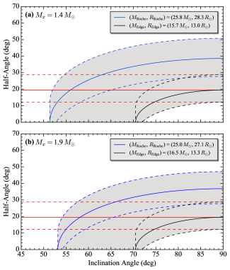
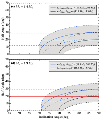
Figure 11.— Predicted eclipse half-angle of IGR J16493–4348 as a function of inclination angle, assuming neutron star masses of 1.4 $M_{\odot}$ in (a) and (c) and 1.9 $M_{\odot}$ in (b) and (d). These constraints are obtained using the orbital parameters from (left) circular solution 1 and (right) eccentric solution 1 in Table 6, together with the asymmetric eclipse model parameters in Table 3 from fitting the Swift BAT transient monitor (15–50 keV) orbital profile. The solid blue curves are derived using supergiant mass and radius values corresponding to where the donor fills its Roche lobe, and the solid black curves are obtained using supergiant mass and radius values derived for an edge-on orbit. The solid red lines indicate the measured eclipse half-angle in Table 3 from fitting the BAT transient monitor orbital profile. The dashed curves correspond to 1$\sigma$ uncertainties on the eclipse half-angles. The grey shaded regions show the allowed parameter space.

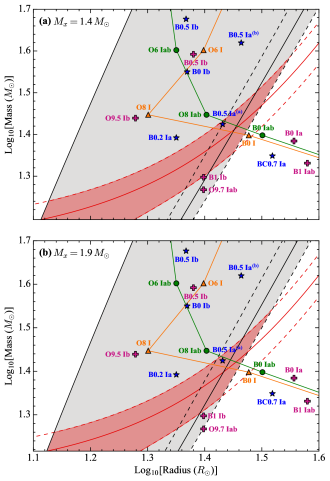
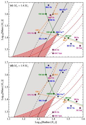
Figure 12.— Log-log plots of stellar mass as a function of stellar radius for IGR J16493–4348’s supergiant companion using the orbital parameters from (left) circular solution 1 and (right) eccentric solution 1 in Table 6. We assume neutron star masses of 1.4 $M_{\odot}$ in (a) and (c) and 1.9 $M_{\odot}$ in (b) and (d). The left and right solid black curves show constraints corresponding to an edge-on orbit and where the supergiant fills its Roche lobe, respectively. The solid red curves show constraints obtained using the orbital parameters in Table 6 and the asymmetric eclipse model parameters in Table 3 from fitting the Swift BAT transient monitor (15–50 keV) orbital profile. The dashed curves indicate 1$\sigma$ uncertainties on these constraints. The grey shaded regions correspond to the allowed parameter space for inclination angles between Roche lobe overflow and an edge-on orbit, and the red shaded areas indicate the joint allowed region also satisfying constraints from the asymmetric eclipse and timing models. The green circles, orange triangles, blue stars, and magenta crosses correspond to supergiant spectral types from Carroll & Ostlie (2006), Cox (2000), Searle et al. (2008), and Lefever et al. (2007), respectively. The B0.5 Ia${}^{\text{(a)}}$ and B0.5 Ia${}^{\text{(b)}}$ labels are used to distinguish between the two B0.5 Ia Galactic B supergiants with different masses and radii in Table 3 of Searle et al. (2008). We favor a spectral type of B0.5 Ia for the supergiant donor since this is the only spectral type that lies in the joint allowed regions derived using the orbital parameters from circular solution 1.

Table 8System Parameters of IGR J16493–4348 for Selected Spectral Types

Spectral Type	$M_{c}$a	$q$b	$R_{c}$c	$R_{L}$d	$\beta$e	$i$f	$M_{V}$g	$(J-K)_{0}$h	$E(J-K)$i	$d$j	$N_{\text{H}}$k
	$(M_{\odot})$		$(R_{\odot})$	$(R_{\odot})$		(deg)	(mag)	(mag)	(mag)	(kpc)	(10${}^{\text{22}}$ cm${}^{\text{2}}$)
lO8 Iab	28.0	0.05	25.3	29.3	0.86	62.9${}^{\text{+6.4}}_{\text{--5.0}}$	–6.6	–0.18 $\pm$ 0.13	2.84 $\pm$ 0.15	14.8 $\pm$ 1.2	3.00 $\pm$ 0.25
mB0.2 Ia	24.7 $\pm$ 7.1	0.06 $\pm$ 0.02	22.4 $\pm$ 3.2	27.8 $\pm$ 2.7	0.81 $\pm$ 0.14	66.7${}^{\text{+10.7}}_{\text{--9.7}}$	–6.07 $\pm$ 0.30	–0.13 $\pm$ 0.13	2.79 $\pm$ 0.15	12.9 $\pm$ 2.1	2.94 $\pm$ 0.24
mB0.5 Ia${}^{\text{(a)}}$	26.6 $\pm$ 2.4	0.053 $\pm$ 0.005	27.0 $\pm$ 1.2	28.7 $\pm$ 0.9	0.94 $\pm$ 0.05	59.0${}^{+6.1}_{-5.1}$	–6.48 $\pm$ 0.10	–0.12 $\pm$ 0.13	2.78 $\pm$ 0.15	16.1 $\pm$ 1.5	2.93 $\pm$ 0.24
mB0.5 Ia${}^{\text{(b)}}$	41.6 $\pm$ 3.8	0.034 $\pm$ 0.003	29.1 $\pm$ 1.3	34.7 $\pm$ 1.1	0.84 $\pm$ 0.05	62.3${}^{\text{+6.8}}_{\text{--5.6}}$	–6.54 $\pm$ 0.10	–0.12 $\pm$ 0.13	2.78 $\pm$ 0.15	16.5 $\pm$ 1.6	2.93 $\pm$ 0.24
mB0.5 Ib	47.5 $\pm$ 8.8	0.029 $\pm$ 0.005	23.3 $\pm$ 2.2	36.6 $\pm$ 2.3	0.64 $\pm$ 0.07	74.1${}^{\text{+12.4}}_{\text{--10.2}}$	–6.36 $\pm$ 0.20	–0.12 $\pm$ 0.13	2.78 $\pm$ 0.15	15.3 $\pm$ 1.9	2.93 $\pm$ 0.24
nB1 Ib	19.8	0.07	25.0	25.3	0.99	58.2${}^{\text{+5.3}}_{\text{--4.2}}$	–5.8	–0.13 $\pm$ 0.13	2.79 $\pm$ 0.15	11.9 $\pm$ 1.0	2.94 $\pm$ 0.24

Note. — System parameters for selected spectral types from Carroll & Ostlie (2006), Searle et al. (2008), and Lefever et al. (2007). We assumed a canonical neutron star mass of 1.4 $M_{\odot}$ and used the orbital parameters from circular solution 1 in Table 6 and the eclipse half-angle in Table 3 from fitting the Swift BAT transient monitor (15–50 keV) orbital profile with an asymmetric eclipse model. We report 1$\sigma$ uncertainties on these parameters, if applicable. The favored supergiant spectral type from the stellar mass-radius diagrams in Figure 12 is highlighted in bold.

^a Mass of the supergiant companion from Carroll & Ostlie (2006), Searle et al. (2008), and Lefever et al. (2007).

^b Mass ratio, $q$ $=$ $M_{x}/M_{c}$, where $M_{x}$ is the neutron star mass and $M_{c}$ is the mass of the supergiant donor.

^c Radius of the supergiant companion from Carroll & Ostlie (2006), Searle et al. (2008), and Lefever et al. (2007).

^d Roche lobe radius calculated using Equation (23).

^e Roche lobe filling factor, $\beta$ $=$ $R_{c}/R_{L}$, where $R_{c}$ is radius of the supergiant donor and $R_{L}$ is the Roche lobe radius.

^f Inclination angle calculated using Equation (22).

^g Absolute magnitude from Carroll & Ostlie (2006), Searle et al. (2008), and Lefever et al. (2007).

^h $(J-K)_{0}$ intrinsic color index calculated using the $(J-V)_{0}$ and $(K-V)_{0}$ color indices from Wegner (1994). The uncertainties on the intrinsic color indices were calculated using Equation (6) in Wegner (1994).

ⁱ Excess color calculated by subtracting the intrinsic $(J-K)_{0}$ color from the $(J-K)_{\text{2MASS}}$ color.

^j Distance to the source calculated using the distance modulus with an apparent 2MASS $K$-band magnitude from Cutri et al. (2003) and $K$-band extinction determined from Rieke & Lebofsky (1985).

^k Hydrogen column density calculated from the correlation with visual extinction in Predehl & Schmitt (1995).

^l Supergiant star from Carroll & Ostlie (2006).

^m Supergiant star from Searle et al. (2008).

ⁿ Supergiant star from Lefever et al. (2007).

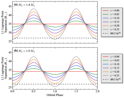
Figure 13.— L1 Lagrange point separation from IGR J16493–4348’s supergiant companion as a function of orbital phase. The solid curves indicate the separation for different eccentricities between 0 and 0.25, and the horizontal dashed lines correspond to a supergiant radius of 27 $R_{\odot}$ for the favored B0.5 Ia spectral type from Searle et al. (2008). For eccentric orbits with $e$ $\gtrsim$ 0.20, Roche lobe overflow will be induced during orbital phases where the L1 Lagrange point separation is inside the supergiant.

5. Discussion

5.1. Donor Star Spectral Type

Our measurements of the 6.78 day orbital period and 1093 s pulse period firmly place IGR J16493–4348 in the wind-fed sgHMXB region of the $P_{\text{orb}}$–$P_{\text{pulse}}$ Corbet diagram (Corbet, 1984, 1986). This is further supported by comparing our X-ray mass function of $f_{x}(M)$ $=$ 13.2${}^{\text{+2.4}}_{\text{--2.5}}$ $M_{\odot}$ to the X-ray mass functions of other sgHMXBs (Townsend et al., 2011). Nespoli et al. (2010) estimated the spectral type of the donor star to be a B0.5-1 Ia-Ib supergiant by comparing the relative strength of He I lines from $K_{\text{S}}$-band spectroscopy of IGR J16493–4348’s infrared companion to those reported in Hanson et al. (1996). We find a spectral type of B0.5 Ia for the supergiant companion using constraints derived in the stellar mass-radius diagrams shown in Figure 12. We assumed neutron star masses of 1.4 $M_{\odot}$ and 1.9 $M_{\odot}$ since neither optical nor infrared radial velocity semi-amplitude measurements were available. In both cases, we obtain a spectral type that is consistent with the result in Nespoli et al. (2010), but we note that a compact object of 1.9 $M_{\odot}$ would make it one of the most massive neutron stars in an X-ray binary (van Kerkwijk et al., 1995; Kaper et al., 2006). Two Galactic B supergiants with spectral types of B0.5 Ia from Searle et al. (2008) are shown in Figure 12, but constraints on the allowed mass and radius from our timing models exclude the more massive, larger donor. From our spectral classification, we estimate the surface effective temperature and luminosity to be approximately 26,000 K and 3.0 $\times$ 10${}^{5}\,L_{\odot}$, respectively.

We estimate the distance to the source using the supergiant’s B0.5 Ia spectral type and the reported parameters in Table 3 of Searle et al. (2008). The infrared counterpart has an apparent $K$-band magnitude of $m_{K}$ $=$ 11.94 $\pm$ 0.04 from 2MASS photometry (Cutri et al., 2003). An absolute $K$-band magnitude of $M_{K}$ $=$ –5.93 $\pm$ 0.14 was derived from the absolute $V$-band magnitude of $M_{V}$ $=$ –6.48 $\pm$ 0.10 in Searle et al. (2008) and the intrinsic $(K-V)_{0}$ color index of 0.55 $\pm$ 0.10 in Wegner (1994). Next, we found the instrinsic $(J-K)_{0}$ color index to be –0.12 $\pm$ 0.13 using the $(J-V)_{0}$ and $(K-V)_{0}$ color indices from Wegner (1994). An $E(J-K)$ color excess of 2.78 $\pm$ 0.15 was obtained by subtracting the intrinsic color $(J-K)_{0}$ from the $(J-K)_{\text{2MASS}}$ color. Assuming an average extincition of $R_{V}$ $=$ 3.09 $\pm$ 0.03, we found a $V$-band extinction magnitude of $A_{V}$ $=$ 16.4 $\pm$ 1.3 from the relation $A_{V}/E(J-K)$ $=$ 5.90 $\pm$ 0.36 (Rieke & Lebofsky, 1985). This yielded an extinction magnitude of $A_{K}$ $=$ 1.8 $\pm$ 0.1 at $K$-band using $A_{K}/A_{V}$ $=$ 0.112 from Table 3 in Rieke & Lebofsky (1985). From the distance modulus, $M_{K}$ $=$ $m_{K}$ $+$ $5$ $-$ $5$ $\mathrm{log}\,d$ $-$ $A_{K}$, we find that IGR J16493–4348 lies at a distance of 16.1 $\pm$ 1.5 kpc, which is consistent with the 6–26 kpc distance estimate in Nespoli et al. (2010). Our distance measurement is also in agreement with the 7.5–22 kpc distance reported by Hill et al. (2008) from infrared spectral energy distribution measurements of the supergiant companion.

Next, we calculate a hydrogen column density of $N_{\text{H}}$ $=$ (2.93 $\pm$ 0.24) $\times$ 10${}^{\text{22}}$ cm${}^{\text{--2}}$ from the correlation between visual extinction and hydrogen column density in Predehl & Schmitt (1995), which is consistent with the estimate given in Nespoli et al. (2010). If we instead use the more recently measured correlation between optical extinction and $N_{\text{H}}$ in Güver & Özel (2009), we obtain a hydrogen column density of $N_{\text{H}}$ $=$ (3.62 $\pm$ 0.33) $\times$ 10${}^{\text{22}}$ cm${}^{\text{--2}}$. Using the procedure in Willingale et al. (2013), we find a total hydrogen column density of $N_{\text{H}}$ $=$ 1.56 $\times$ 10${}^{\text{22}}$ cm${}^{\text{--2}}$, which is comparable to the $N_{\text{H}}$ values of 1.42 $\times$ 10${}^{\text{22}}$ cm${}^{\text{--2}}$ and 1.82 $\times$ 10${}^{\text{22}}$ cm${}^{\text{--2}}$ obtained from the Leiden/Argentine/Bonn survey (Kalberla et al., 2005) and Dickey & Lockman (1990), respectively, using measurements of H I in the Galaxy. We note that all of these values are smaller than the observed hydrogen column densities measured by Hill et al. (2008), Morris et al. (2009), D’Aì et al. (2011), and Coley et al. (2018). Spectral analyses in the soft and hard X-ray bands have found hydrogen column densities ranging between roughly 5–10 $\times$ 10${}^{\text{22}}$ cm${}^{\text{--2}}$ on average. This suggests that there may be an additional component of the hydrogen absorbing column that is intrinsic to the system.

5.2. Eclipse Asymmetry

Asymmetry in the X-ray eclipse profile is often a signature of a photoionization wake (Fransson & Fabian, 1980; Feldmeier et al., 1996), accretion bow shock and/or accretion wake trailing the neutron star (Blondin et al., 1990, 1991), or other complex structure in the stellar wind. We discuss these phenomena and argue that a strong photoionization or accretion wake is not supported by the X-ray emission observed from IGR J16493–4348.

Mass transfer onto the neutron star occurs through the radiatively powered stellar wind of the supergiant companion. X-ray photoionization can result in collisions between the compressed, ionized gas and the accelerating wind, which causes shocks and dense regions of compressed gas from the wind to trail the X-ray source in its orbit around the supergiant (Jackson, 1975; Fransson & Fabian, 1980). In systems with high X-ray luminosities, the wind is highly ionized in the vicinity of the X-ray source, and the radiative driving force powering the stellar wind is significantly reduced near the surface of the supergiant (Feldmeier et al., 1996). As seen in Vela X-1 (Feldmeier et al., 1996), the dense gas trailing the photoionization wake can lead to X-ray photoelectric absorption at orbital phases prior to the eclipse and X-ray scattering into the observer’s line of sight after eclipse ingress. This can produce ingress durations that are longer than those observed at egress.

Dense regions of compressed gas in the accretion bow shock and/or accretion wake of the compact object can also induce phase-dependent photoelectric absorption (Jackson, 1975; Blondin et al., 1990, 1991). This leads to an enhancement in the hydrogen column density and absorption of the X-ray emission prior to the eclipse (Manousakis & Walter, 2015). No apparent increase in the hydrogen column density is observable during egress when the accretion wake is located beyond the compact object. We do not find evidence of a strong photoionization or accretion wake since there are no statistically significant differences between the ingress and egress durations or the count rates near ingress and egress in the PCA scan or BAT orbital profiles.

The eclipse profile structure is often dependent on X-ray photon energy. For example, Jain et al. (2009) found that the X-ray eclipses from the SFXT IGR J16479–4514 were more evident and exhibited sharper transitions at higher energies using the Swift BAT compared to observations at lower energies with the RXTE All-Sky Monitor (ASM). This type of behavior has also been observed from various other eclipsing systems in the hard X-ray band (e.g., Falanga et al. 2015). These effects are often linked to the absorbing column density, which causes increased X-ray absorption and scattering at softer X-ray energies. Although the eclipse duration of IGR J16493–4348 was consistent between the PCA scan and BAT orbital profiles, there are observable differences in the eclipse profile structure across the X-ray energy band (see Figure 7). While these differences may be indicative of energy dependent structure in the eclipses, systematic effects from binning could also affect the observed eclipse shape.

5.3. Orbital Eccentricity

Previous estimates by Cusumano et al. (2010) suggest that the orbital eccentricity cannot exceed 0.15 based on IGR J16493–4348’s classification as a wind-fed sgHMXB. An eccentricity of $e$ $=$ 0.17 $\pm$ 0.09 was measured using the timing model in eccentric solution 1. While this eccentricity is consistent with the upper limit presented in Cusumano et al. (2010), we suspect that the orbit is nearly circular since the ToAs are well modeled by circular solution 1 and a B0.5 Ia spectral type fell within the joint allowed parameter space in the corresponding stellar mass-radius diagrams in Figure 12. This spectral type is also consistent with the spectral classification given by Nespoli et al. (2010). Additionally, no spectral types were found inside the joint allowed regions obtained using eccentric solution 1. If the orbit were highly eccentric ($e$ $\gtrsim$ 0.20), then the L1 Lagrange point separation from the supergiant would be located inside the donor during a fraction of the orbit, which would lead to Roche lobe overflow and inhibit mass transfer via the stellar wind. Since the eccentric timing model fits have only a few degrees of freedom, higher cadence pulsar timing observations over multiple orbital cycles are needed to measure the system’s eccentricity and longitude of periastron more accurately.

We compare the mid-eclipse time predicted by eccentric solution 1 in Table 6 to the measured mid-eclipse times from the PCA scan and BAT orbital profiles in Tables 3 and 4. To first order in $e$, the time of mid-eclipse in an eccentric orbit is given by (van der Klis & Bonnet-Bidaud, 1984; Falanga et al., 2015):

$$T_{\text{mid}}=T_{\pi/2}-\frac{eP_{\text{orb}}}{\pi}\cos\omega$$ (24)

Here, $T_{\pi/2}$ is calculated from the periastron passage time, $T_{\text{peri}}$, using (van der Klis & Bonnet-Bidaud, 1984):

$$T_{\pi/2}=T_{\text{peri}}+\frac{P_{\text{orb}}}{2\pi}\left(\frac{\pi}{2}-\omega\right)$$ (25)

If the orbit is circular, the values of $T_{\pi/2}$ and $T_{\text{mid}}$ will coincide.

Substituting the orbital parameters from eccentric solution 1 into Equations (24) and (25), we find that $T_{\pi/2}$ $=$ MJD 55850.9 $\pm$ 0.8 and $T_{\text{mid}}$ $=$ MJD 55851.0 $\pm$ 0.8 are consistent with each other. The large uncertainties in these calculated values are attributed to the broad posterior distributions measured for the periastron passage time and longitude of periastron in eccentric solution 1. This calculated mid-eclipse time agrees with all of the measured mid-eclipse times in Tables 3 and 4 to within 1$\sigma$. In addition, the value of $T_{\pi/2}$ derived from eccentric solution 1 is consistent with the values of $T_{\pi/2}$ measured using the circular timing models in Table 6. This further supports the notion that the orbit is likely not highly eccentric.

5.4. Superorbital Mechanisms

IGR J16493–4348 is one of only five wind-fed sgHMXB systems in which superorbital modulation has been definitively observed (e.g., 2S 0114+650, 4U 1909+07, IGR J16418–4532, and IGR J16479–4514; Corbet & Krimm 2013). In addition, Corbet et al. (2018) recently reported apparent superorbital modulation from the eclipsing sgHMXB, 4U 1538–52. Superorbital variability from other X-ray pulsar binaries, such as Her X-1, SMC X-1, and LMC X-4, has been linked to mass flow onto the accretion disk of the neutron star via Roche lobe overflow (Clarkson et al., 2003a, b). Accretion flow onto the surface of a freely precessing neutron star with a complex non-dipole magnetic field has also been suggested to explain the 35 day superorbital period of Her X-1 (Postnov et al., 2013). Alternatively, the periodic superorbital behavior in these systems could be caused by a twisted, warped precessing accretion disk (Petterson, 1975; Wojdowski et al., 1998; Ogilvie & Dubus, 2001; Hung et al., 2010).

We detected coherent superorbital modulation at a period of 20.07 days from semi-weighted DFTs of the BAT and PCA scan light curves. While superorbital periods of similar length have been detected in other wind accreting sgHMXBs, such as 2S 0114+650, the mechanism responsible for the variability still has not been clearly identified (Farrell et al., 2006; Masetti et al., 2006; Farrell et al., 2008; Hu et al., 2017). It may be possible that tidal oscillations from IGR J16493–4348’s B0.5 Ia supergiant companion are driving the variability if the orbit is indeed circular (Koenigsberger et al., 2003; Moreno et al., 2005; Koenigsberger et al., 2006). Using a tidal interaction model, Koenigsberger et al. (2006) found that these oscillations would produce modulation on superorbital timescales in binary systems with circular orbits, while orbital period length variability would be observed if these oscillations occurred in eccentric orbits. In both cases, suborbital variability was also predicted on shorter timescales. This may suggest that the mechanism responsible for the superorbital modulation is the structured stellar wind of the supergiant companion, possibly along with X-ray emission generated by strong perturbations on the surface layers of the donor star.

Alternatively, the superorbital variability may be related to the presence of corotating interaction regions (CIRs) in the stellar wind of the supergiant (Bozzo et al., 2017). These structures are thought to form from irregularities on the surface of the donor star and are located at radial distances of tens of stellar radii (Mullan, 1984; Cranmer & Owocki, 1996). We find that IGR J16493-4348’s superorbital period is persistently detected in X-ray observations spanning several years, but its strength is variable in time (Coley et al., 2018). This implies that these CIRs would have to be stable over long timescales if this is the dominant mechanism driving the variability, which has not yet been established. A detailed discussion of other possible mechanisms responsible for the superorbital modulation is presented in Coley et al. (2018).

6. Conclusion

IGR J16493–4348 is an eclipsing, wind-fed sgHMXB with an early B-type supergiant companion. We refine the superorbital period to 20.067 $\pm$ 0.009 days from a semi-weighted DFT of the BAT transient monitor light curve. An improved orbital period measurement of 6.7828 $\pm$ 0.0004 days is obtained from an O–C analysis using the PCA scan and BAT transient monitor data. Asymmetric and symmetric eclipse models were fit to the PCA scan and BAT orbital profiles, and no evidence of a strong photoionization or accretion wake was found.

Pulsations were detected in the unweighted power spectrum of the pointed PCA light curve after the removal of low frequency noise. We refine the pulse period to 1093.1036 $\pm$ 0.0004 s from a pulsar timing analysis using the pointed PCA data. The system’s Keplerian binary orbital parameters were measured by fitting circular and eccentric timing models to the ToAs. We find that the orbit is likely nearly circular, and no significant change in the rotational period of the pulsar was observed. A mass function of $f_{x}(M)$ $=$ 13.2${}^{\text{+2.4}}_{\text{--2.5}}$ $M_{\odot}$ was derived from the binary orbital parameters, which allows us to definitively classify IGR J16493–4348 as an sgHMXB. This is further supported by its updated placement in the wind-fed sgHMXB region of the $P_{\text{orb}}$–$P_{\text{pulse}}$ Corbet diagram. We derive new constraints on the mass and radius of the donor star, which indicate a B0.5 Ia spectral type for the supergiant companion. Additional parameters describing the system geometry are also provided, which give insight into possible inclination angles and Roche lobe sizes.

Although we argue that the binary follows a nearly circular orbit, additional ToAs are needed to provide improved constraints on the system’s eccentricity and longitude of periastron. Optical or infrared radial velocity measurements would directly determine the pulsar’s neutron star mass, which would allow the system to be classified as a double-lined eclipsing binary. The driving mechanism behind the superorbital modulation remains unexplained, but it is currently thought to be linked with the stellar wind of the supergiant companion.

Appendix

In Table 9, we provide a complete list of calculated values for the companion mass, mass ratio, companion radius, Roche lobe radius, and Roche lobe filling factor using the orbital parameters from each timing solution in Table 6 and the asymmetric and symmetric eclipse model parameters in Tables 3 and 4 from fitting the folded BAT transient monitor and PCA scan orbital profiles. These values were determined at inclination angles corresponding to Roche lobe overflow and an edge-on orbit. We assumed neutron star masses of 1.4 $M_{\odot}$ and 1.9 $M_{\odot}$ in these calculations.

Table 9Supergiant Donor Parameters of IGR J16493–4348

Parameter	Circular Solution 1		Circular Solution 2		Circular Solution 3		Eccentric Solution 1		Eccentric Solution 2
Swift BAT Transient Monitor (15–50 keV), Asymmetric Eclipse Model
$i$ (deg)a	56.0${}^{\text{+6.4}}_{\text{--5.8}}$	90.0	56.0${}^{\text{+6.1}}_{\text{--5.6}}$	90.0	56.4${}^{\text{+5.9}}_{\text{--5.3}}$	90.0	67.8${}^{\text{+9.2}}_{\text{--8.3}}$	90.0	68.2${}^{\text{+10.7}}_{\text{--9.7}}$	90.0
$M_{x}$ $(M_{\odot})$b	1.4	1.4	1.4	1.4	1.4	1.4	1.4	1.4	1.4	1.4
$M_{c}$ $(M_{\odot})$c	25.8${}^{\text{+6.3}}_{\text{--5.9}}$	15.7${}^{\text{+2.4}}_{\text{--2.5}}$	25.7${}^{\text{+6.2}}_{\text{--5.9}}$	15.6${}^{\text{+2.8}}_{\text{--2.9}}$	24.3${}^{\text{+5.5}}_{\text{--5.2}}$	15.0${}^{\text{+2.6}}_{\text{--2.7}}$	19.3${}^{\text{+4.2}}_{\text{--3.9}}$	15.8${}^{\text{+2.5}}_{\text{--2.6}}$	18.8${}^{\text{+4.8}}_{\text{--4.5}}$	15.5 $\pm$ 2.7
$q$d	0.05 $\pm$ 0.01	0.09 $\pm$ 0.01	0.05 $\pm$ 0.01	0.09 $\pm$ 0.02	0.06 $\pm$ 0.01	0.09 $\pm$ 0.02	0.07${}^{\text{+0.02}}_{\text{--0.01}}$	0.09 $\pm$ 0.01	0.07 $\pm$ 0.02	0.09 $\pm$ 0.02
$R_{c}$ $(R_{\odot})$e	28.3${}^{\text{+5.7}}_{\text{--5.1}}$	13.0${}^{\text{+5.9}}_{\text{--4.7}}$	28.3${}^{\text{+5.4}}_{\text{--4.9}}$	13.0${}^{\text{+5.9}}_{\text{--4.7}}$	27.6${}^{\text{+5.1}}_{\text{--4.6}}$	12.8${}^{\text{+5.8}}_{\text{--4.6}}$	20.8${}^{\text{+6.4}}_{\text{--5.7}}$	13.3${}^{\text{+6.2}}_{\text{--5.0}}$	20.4${}^{\text{+7.4}}_{\text{--6.5}}$	13.3${}^{\text{+6.2}}_{\text{--4.9}}$
$R_{L}$ $(R_{\odot})$f	28.3${}^{\text{+2.8}}_{\text{--2.6}}$	22.8 $\pm$ 1.2	28.3${}^{\text{+2.7}}_{\text{--2.6}}$	22.8${}^{\text{+1.3}}_{\text{--1.4}}$	27.6${}^{\text{+2.5}}_{\text{--2.3}}$	22.3 $\pm$ 1.3	20.8 $\pm$ 2.5	19.0${}^{\text{+2.2}}_{\text{--2.4}}$	20.4${}^{\text{+2.7}}_{\text{--2.8}}$	18.8${}^{\text{+2.1}}_{\text{--2.3}}$
$\beta$g	1.00${}^{\text{+0.22}}_{\text{--0.20}}$	0.57${}^{\text{+0.26}}_{\text{--0.21}}$	1.00${}^{\text{+0.22}}_{\text{--0.20}}$	0.57${}^{\text{+0.26}}_{\text{--0.21}}$	1.00${}^{\text{+0.21}}_{\text{--0.19}}$	0.57${}^{\text{+0.26}}_{\text{--0.21}}$	1.00${}^{\text{+0.33}}_{\text{--0.30}}$	0.70${}^{\text{+0.34}}_{\text{--0.27}}$	1.00${}^{\text{+0.39}}_{\text{--0.35}}$	0.71${}^{\text{+0.34}}_{\text{--0.28}}$
$i$ (deg)a	58.1${}^{\text{+5.9}}_{\text{--5.1}}$	90.0	58.1${}^{\text{+7.8}}_{\text{--6.9}}$	90.0	58.5${}^{\text{+7.5}}_{\text{--6.6}}$	90.0	69.4${}^{\text{+8.6}}_{\text{--7.6}}$	90.0	69.9${}^{\text{+10.1}}_{\text{--9.0}}$	90.0
$M_{x}$ $(M_{\odot})$b	1.9	1.9	1.9	1.9	1.9	1.9	1.9	1.9	1.9	1.9
$M_{c}$ $(M_{\odot})$c	25.0${}^{\text{+5.1}}_{\text{--4.8}}$	16.5 $\pm$ 2.5	24.9${}^{\text{+7.0}}_{\text{--6.6}}$	16.4${}^{\text{+2.8}}_{\text{--2.9}}$	23.6${}^{\text{+6.2}}_{\text{--5.8}}$	15.7 $\pm$ 2.7	19.5${}^{\text{+3.6}}_{\text{--3.3}}$	16.5 $\pm$ 2.6	19.0${}^{\text{+4.1}}_{\text{--3.9}}$	16.3 $\pm$ 2.7
$q$d	0.08${}^{\text{+0.02}}_{\text{--0.01}}$	0.12 $\pm$ 0.02	0.08 $\pm$ 0.02	0.12 $\pm$ 0.02	0.08 $\pm$ 0.02	0.12 $\pm$ 0.02	0.10 $\pm$ 0.02	0.11 $\pm$ 0.02	0.10 $\pm$ 0.02	0.12 $\pm$ 0.02
$R_{c}$ $(R_{\odot})$e	27.1${}^{\text{+5.0}}_{\text{--4.4}}$	13.3${}^{\text{+6.1}}_{\text{--4.8}}$	27.0${}^{\text{+6.6}}_{\text{--5.9}}$	13.3${}^{\text{+6.1}}_{\text{--4.8}}$	26.4${}^{\text{+6.3}}_{\text{--5.5}}$	13.1${}^{\text{+6.0}}_{\text{--4.7}}$	20.2${}^{\text{+5.9}}_{\text{--5.1}}$	13.7${}^{\text{+6.4}}_{\text{--5.1}}$	19.9${}^{\text{+6.8}}_{\text{--5.9}}$	13.6${}^{\text{+6.3}}_{\text{--5.0}}$
$R_{L}$ $(R_{\odot})$f	27.1${}^{\text{+2.2}}_{\text{--2.1}}$	22.6${}^{\text{+1.1}}_{\text{--1.2}}$	27.0${}^{\text{+3.0}}_{\text{--2.8}}$	22.5 $\pm$ 1.3	26.4${}^{\text{+2.8}}_{\text{--2.6}}$	22.1 $\pm$ 1.2	20.2 $\pm$ 2.1	18.8${}^{\text{+2.2}}_{\text{--2.3}}$	19.9${}^{\text{+2.3}}_{\text{--2.4}}$	18.6${}^{\text{+2.0}}_{\text{--2.3}}$
$\beta$g	1.00${}^{\text{+0.20}}_{\text{--0.18}}$	0.59${}^{\text{+0.27}}_{\text{--0.22}}$	1.00${}^{\text{+0.27}}_{\text{--0.24}}$	0.59${}^{\text{+0.27}}_{\text{--0.22}}$	1.00${}^{\text{+0.26}}_{\text{--0.23}}$	0.59${}^{\text{+0.27}}_{\text{--0.22}}$	1.00${}^{\text{+0.31}}_{\text{--0.27}}$	0.73${}^{\text{+0.35}}_{\text{--0.28}}$	1.00${}^{\text{+0.36}}_{\text{--0.32}}$	0.73${}^{\text{+0.35}}_{\text{--0.29}}$
RXTE PCA Galactic Bulge Scans (2–10 keV), Asymmetric Eclipse Model
$i$ (deg)a	58.5${}^{\text{+4.9}}_{\text{--5.1}}$	90.0	58.6${}^{\text{+4.7}}_{\text{--4.8}}$	90.0	59.0 $\pm$ 5.5	90.0	71.8${}^{\text{+9.7}}_{\text{--10.1}}$	90.0	72.3${}^{\text{+6.9}}_{\text{--7.4}}$	90.0
$M_{x}$ $(M_{\odot})$b	1.4	1.4	1.4	1.4	1.4	1.4	1.4	1.4	1.4	1.4
$M_{c}$ $(M_{\odot})$c	23.9${}^{\text{+4.7}}_{\text{--4.9}}$	15.7${}^{\text{+2.4}}_{\text{--2.5}}$	23.8${}^{\text{+4.5}}_{\text{--4.6}}$	15.6${}^{\text{+2.8}}_{\text{--2.9}}$	22.5${}^{\text{+4.9}}_{\text{--5.0}}$	15.0${}^{\text{+2.6}}_{\text{--2.7}}$	18.0${}^{\text{+3.9}}_{\text{--4.0}}$	15.8${}^{\text{+2.5}}_{\text{--2.6}}$	17.6${}^{\text{+2.8}}_{\text{--2.9}}$	15.5 $\pm$ 2.7
$q$d	0.06 $\pm$ 0.01	0.09 $\pm$ 0.01	0.06 $\pm$ 0.01	0.09 $\pm$ 0.02	0.06 $\pm$ 0.01	0.09 $\pm$ 0.02	0.08 $\pm$ 0.02	0.09 $\pm$ 0.01	0.08 $\pm$ 0.01	0.09 $\pm$ 0.02
$R_{c}$ $(R_{\odot})$e	27.4${}^{\text{+3.8}}_{\text{--4.0}}$	15.1${}^{\text{+1.8}}_{\text{--1.9}}$	27.3${}^{\text{+3.6}}_{\text{--3.7}}$	15.1${}^{\text{+1.9}}_{\text{--2.0}}$	26.7${}^{\text{+4.1}}_{\text{--4.2}}$	14.9${}^{\text{+1.8}}_{\text{--1.9}}$	20.2${}^{\text{+5.1}}_{\text{--5.3}}$	15.6${}^{\text{+2.3}}_{\text{--2.4}}$	19.8${}^{\text{+3.6}}_{\text{--3.8}}$	15.5 $\pm$ 2.3
$R_{L}$ $(R_{\odot})$f	27.4${}^{\text{+2.1}}_{\text{--2.2}}$	22.8 $\pm$ 1.2	27.3${}^{\text{+2.0}}_{\text{--2.1}}$	22.8${}^{\text{+1.3}}_{\text{--1.4}}$	26.7${}^{\text{+2.2}}_{\text{--2.3}}$	22.3 $\pm$ 1.3	20.2${}^{\text{+2.7}}_{\text{--2.8}}$	19.0${}^{\text{+2.2}}_{\text{--2.4}}$	19.8${}^{\text{+1.8}}_{\text{--2.0}}$	18.8${}^{\text{+2.1}}_{\text{--2.3}}$
$\beta$g	1.00${}^{\text{+0.16}}_{\text{--0.17}}$	0.66 $\pm$ 0.09	1.00${}^{\text{+0.15}}_{\text{--0.16}}$	0.66 $\pm$ 0.09	1.00${}^{\text{+0.17}}_{\text{--0.18}}$	0.67 $\pm$ 0.09	1.00${}^{\text{+0.29}}_{\text{--0.30}}$	0.82${}^{\text{+0.15}}_{\text{--0.16}}$	1.00${}^{\text{+0.20}}_{\text{--0.22}}$	0.82${}^{\text{+0.15}}_{\text{--0.16}}$
$i$ (deg)a	60.9${}^{\text{+4.2}}_{\text{--4.4}}$	90.0	60.9${}^{\text{+5.7}}_{\text{--5.9}}$	90.0	61.3${}^{\text{+4.9}}_{\text{--5.0}}$	90.0	73.8${}^{\text{+7.5}}_{\text{--7.8}}$	90.0	74.4${}^{\text{+7.4}}_{\text{--7.9}}$	90.0
$M_{x}$ $(M_{\odot})$b	1.9	1.9	1.9	1.9	1.9	1.9	1.9	1.9	1.9	1.9
$M_{c}$ $(M_{\odot})$c	23.2${}^{\text{+3.7}}_{\text{--3.9}}$	16.5 $\pm$ 2.5	23.1${}^{\text{+5.1}}_{\text{--5.3}}$	16.4${}^{\text{+2.8}}_{\text{--2.9}}$	21.9${}^{\text{+4.1}}_{\text{--4.2}}$	15.7 $\pm$ 2.7	18.3 $\pm$ 2.8	16.5 $\pm$ 2.6	17.9 $\pm$ 2.8	16.3 $\pm$ 2.7
$q$d	0.08 $\pm$ 0.01	0.12 $\pm$ 0.02	0.08 $\pm$ 0.02	0.12 $\pm$ 0.02	0.09 $\pm$ 0.02	0.12 $\pm$ 0.02	0.10 $\pm$ 0.02	0.11 $\pm$ 0.02	0.11 $\pm$ 0.02	0.12 $\pm$ 0.02
$R_{c}$ $(R_{\odot})$e	26.2${}^{\text{+3.1}}_{\text{--3.2}}$	15.5${}^{\text{+1.8}}_{\text{--1.9}}$	26.2${}^{\text{+4.2}}_{\text{--4.3}}$	15.5${}^{\text{+1.9}}_{\text{--2.0}}$	25.6 $\pm$ 3.5	15.3${}^{\text{+1.8}}_{\text{--1.9}}$	19.7${}^{\text{+3.7}}_{\text{--3.8}}$	15.9${}^{\text{+2.3}}_{\text{--2.4}}$	19.3${}^{\text{+3.6}}_{\text{--3.8}}$	15.9${}^{\text{+2.3}}_{\text{--2.4}}$
$R_{L}$ $(R_{\odot})$f	26.2${}^{\text{+1.6}}_{\text{--1.7}}$	22.6${}^{\text{+1.1}}_{\text{--1.2}}$	26.2${}^{\text{+2.2}}_{\text{--2.3}}$	22.5 $\pm$ 1.3	25.6 $\pm$ 1.8	22.1 $\pm$ 1.2	19.7${}^{\text{+1.9}}_{\text{--2.0}}$	18.8${}^{\text{+2.2}}_{\text{--2.3}}$	19.3${}^{\text{+1.7}}_{\text{--2.0}}$	18.6${}^{\text{+2.0}}_{\text{--2.3}}$
$\beta$g	1.00${}^{\text{+0.13}}_{\text{--0.14}}$	0.69 $\pm$ 0.09	1.00${}^{\text{+0.18}}_{\text{--0.19}}$	0.69${}^{\text{+0.09}}_{\text{--0.10}}$	1.00${}^{\text{+0.15}}_{\text{--0.16}}$	0.69${}^{\text{+0.09}}_{\text{--0.10}}$	1.00${}^{\text{+0.21}}_{\text{--0.22}}$	0.85 $\pm$ 0.16	1.00${}^{\text{+0.21}}_{\text{--0.22}}$	0.85${}^{\text{+0.16}}_{\text{--0.17}}$
Swift BAT Transient Monitor (15–50 keV), Symmetric Eclipse Model
$i$ (deg)a	56.3${}^{\text{+5.6}}_{\text{--5.4}}$	90.0	56.3${}^{\text{+5.7}}_{\text{--5.5}}$	90.0	56.6${}^{\text{+6.4}}_{\text{--6.1}}$	90.0	68.2${}^{\text{+7.7}}_{\text{--7.4}}$	90.0	68.6${}^{\text{+9.0}}_{\text{--8.8}}$	90.0
$M_{x}$ $(M_{\odot})$b	1.4	1.4	1.4	1.4	1.4	1.4	1.4	1.4	1.4	1.4
$M_{c}$ $(M_{\odot})$c	25.6 $\pm$ 5.8	15.7${}^{\text{+2.4}}_{\text{--2.5}}$	25.5 $\pm$ 5.9	15.6${}^{\text{+2.8}}_{\text{--2.9}}$	24.1${}^{\text{+6.2}}_{\text{--6.1}}$	15.0${}^{\text{+2.6}}_{\text{--2.7}}$	19.2${}^{\text{+3.7}}_{\text{--3.6}}$	15.8${}^{\text{+2.5}}_{\text{--2.6}}$	18.7${}^{\text{+4.3}}_{\text{--4.2}}$	15.5 $\pm$ 2.7
$q$d	0.05 $\pm$ 0.01	0.09 $\pm$ 0.01	0.05 $\pm$ 0.01	0.09 $\pm$ 0.02	0.06${}^{\text{+0.02}}_{\text{--0.01}}$	0.09 $\pm$ 0.02	0.07 $\pm$ 0.01	0.09 $\pm$ 0.01	0.08 $\pm$ 0.02	0.09 $\pm$ 0.02
$R_{c}$ $(R_{\odot})$e	28.2${}^{\text{+4.9}}_{\text{--4.7}}$	13.2${}^{\text{+4.0}}_{\text{--3.4}}$	28.2${}^{\text{+4.9}}_{\text{--4.7}}$	13.2${}^{\text{+4.0}}_{\text{--3.4}}$	27.5${}^{\text{+5.4}}_{\text{--5.1}}$	13.0${}^{\text{+3.9}}_{\text{--3.4}}$	20.7${}^{\text{+5.2}}_{\text{--4.9}}$	13.6${}^{\text{+4.2}}_{\text{--3.7}}$	20.4${}^{\text{+5.9}}_{\text{--5.7}}$	13.6${}^{\text{+4.2}}_{\text{--3.7}}$
$R_{L}$ $(R_{\odot})$f	28.2 $\pm$ 2.5	22.8 $\pm$ 1.2	28.2 $\pm$ 2.6	22.8${}^{\text{+1.3}}_{\text{--1.4}}$	27.5${}^{\text{+2.8}}_{\text{--2.7}}$	22.3 $\pm$ 1.3	20.7${}^{\text{+2.3}}_{\text{--2.4}}$	19.0${}^{\text{+2.2}}_{\text{--2.4}}$	20.4${}^{\text{+2.5}}_{\text{--2.7}}$	18.8${}^{\text{+2.1}}_{\text{--2.3}}$
$\beta$g	1.00 $\pm$ 0.19	0.58${}^{\text{+0.18}}_{\text{--0.15}}$	1.00${}^{\text{+0.20}}_{\text{--0.19}}$	0.58${}^{\text{+0.18}}_{\text{--0.15}}$	1.00${}^{\text{+0.22}}_{\text{--0.21}}$	0.58${}^{\text{+0.18}}_{\text{--0.15}}$	1.00${}^{\text{+0.27}}_{\text{--0.26}}$	0.72${}^{\text{+0.24}}_{\text{--0.21}}$	1.00${}^{\text{+0.32}}_{\text{--0.31}}$	0.72${}^{\text{+0.24}}_{\text{--0.21}}$
$i$ (deg)a	58.4${}^{\text{+5.7}}_{\text{--5.5}}$	90.0	58.4${}^{\text{+5.3}}_{\text{--5.0}}$	90.0	58.8${}^{\text{+6.4}}_{\text{--6.0}}$	90.0	69.9${}^{\text{+7.9}}_{\text{--7.6}}$	90.0	70.3${}^{\text{+9.3}}_{\text{--9.0}}$	90.0
$M_{x}$ $(M_{\odot})$b	1.9	1.9	1.9	1.9	1.9	1.9	1.9	1.9	1.9	1.9
$M_{c}$ $(M_{\odot})$c	24.8 $\pm$ 5.3	16.5 $\pm$ 2.5	24.7 $\pm$ 5.0	16.4${}^{\text{+2.8}}_{\text{--2.9}}$	23.4${}^{\text{+5.7}}_{\text{--5.5}}$	15.7 $\pm$ 2.7	19.4${}^{\text{+3.5}}_{\text{--3.4}}$	16.5 $\pm$ 2.6	18.9${}^{\text{+4.1}}_{\text{--4.0}}$	16.3 $\pm$ 2.7
$q$d	0.08 $\pm$ 0.02	0.12 $\pm$ 0.02	0.08 $\pm$ 0.02	0.12 $\pm$ 0.02	0.08 $\pm$ 0.02	0.12 $\pm$ 0.02	0.10 $\pm$ 0.02	0.11 $\pm$ 0.02	0.10 $\pm$ 0.02	0.12 $\pm$ 0.02
$R_{c}$ $(R_{\odot})$e	27.0${}^{\text{+4.8}}_{\text{--4.5}}$	13.6${}^{\text{+4.1}}_{\text{--3.5}}$	26.9${}^{\text{+4.4}}_{\text{--4.2}}$	13.5${}^{\text{+4.1}}_{\text{--3.5}}$	26.3${}^{\text{+5.2}}_{\text{--4.9}}$	13.4${}^{\text{+4.0}}_{\text{--3.4}}$	20.2${}^{\text{+5.1}}_{\text{--4.8}}$	13.9${}^{\text{+4.3}}_{\text{--3.7}}$	19.8${}^{\text{+6.0}}_{\text{--5.7}}$	13.9${}^{\text{+4.3}}_{\text{--3.7}}$
$R_{L}$ $(R_{\odot})$f	27.0${}^{\text{+2.3}}_{\text{--2.2}}$	22.6${}^{\text{+1.1}}_{\text{--1.2}}$	26.9 $\pm$ 2.1	22.5 $\pm$ 1.3	26.3${}^{\text{+2.5}}_{\text{--2.4}}$	22.1 $\pm$ 1.2	20.2 $\pm$ 2.2	18.8${}^{\text{+2.2}}_{\text{--2.3}}$	19.8${}^{\text{+2.4}}_{\text{--2.6}}$	18.6${}^{\text{+2.0}}_{\text{--2.3}}$
$\beta$g	1.00${}^{\text{+0.20}}_{\text{--0.19}}$	0.60${}^{\text{+0.18}}_{\text{--0.16}}$	1.00${}^{\text{+0.18}}_{\text{--0.17}}$	0.60${}^{\text{+0.18}}_{\text{--0.16}}$	1.00${}^{\text{+0.22}}_{\text{--0.21}}$	0.60${}^{\text{+0.18}}_{\text{--0.16}}$	1.00${}^{\text{+0.28}}_{\text{--0.26}}$	0.74${}^{\text{+0.25}}_{\text{--0.22}}$	1.00${}^{\text{+0.32}}_{\text{--0.31}}$	0.75${}^{\text{+0.25}}_{\text{--0.22}}$
RXTE PCA Galactic Bulge Scans (2–10 keV), Symmetric Eclipse Model
$i$ (deg)a	60.0${}^{\text{+4.4}}_{\text{--4.5}}$	90.0	60.1 $\pm$ 5.7	90.0	60.5${}^{\text{+5.1}}_{\text{--5.0}}$	90.0	74.4${}^{\text{+11.2}}_{\text{--11.4}}$	90.0	75.0${}^{\text{+8.3}}_{\text{--8.6}}$	90.0
$M_{x}$ $(M_{\odot})$b	1.4	1.4	1.4	1.4	1.4	1.4	1.4	1.4	1.4	1.4
$M_{c}$ $(M_{\odot})$c	22.9${}^{\text{+3.8}}_{\text{--3.9}}$	15.7${}^{\text{+2.4}}_{\text{--2.5}}$	22.8${}^{\text{+4.9}}_{\text{--5.0}}$	15.6${}^{\text{+2.8}}_{\text{--2.9}}$	21.6 $\pm$ 4.1	15.0${}^{\text{+2.6}}_{\text{--2.7}}$	17.4 $\pm$ 3.7	15.8${}^{\text{+2.5}}_{\text{--2.6}}$	17.0${}^{\text{+2.7}}_{\text{--2.8}}$	15.5 $\pm$ 2.7
$q$d	0.06 $\pm$ 0.01	0.09 $\pm$ 0.01	0.06 $\pm$ 0.01	0.09 $\pm$ 0.02	0.06 $\pm$ 0.01	0.09 $\pm$ 0.02	0.08 $\pm$ 0.02	0.09 $\pm$ 0.01	0.08 $\pm$ 0.01	0.09 $\pm$ 0.02
$R_{c}$ $(R_{\odot})$e	26.9 $\pm$ 3.2	16.1${}^{\text{+1.9}}_{\text{--1.7}}$	26.8 $\pm$ 4.1	16.1${}^{\text{+1.9}}_{\text{--1.8}}$	26.2${}^{\text{+3.6}}_{\text{--3.5}}$	15.9${}^{\text{+1.9}}_{\text{--1.7}}$	19.9${}^{\text{+5.0}}_{\text{--5.1}}$	16.6${}^{\text{+2.4}}_{\text{--2.3}}$	19.5${}^{\text{+3.6}}_{\text{--3.7}}$	16.5${}^{\text{+2.4}}_{\text{--2.2}}$
$R_{L}$ $(R_{\odot})$f	26.9${}^{\text{+1.7}}_{\text{--1.8}}$	22.8 $\pm$ 1.2	26.8${}^{\text{+2.2}}_{\text{--2.3}}$	22.8${}^{\text{+1.3}}_{\text{--1.4}}$	26.2 $\pm$ 1.9	22.3 $\pm$ 1.3	19.9${}^{\text{+2.5}}_{\text{--2.7}}$	19.0${}^{\text{+2.2}}_{\text{--2.4}}$	19.5${}^{\text{+1.8}}_{\text{--1.9}}$	18.8${}^{\text{+2.1}}_{\text{--2.3}}$
$\beta$g	1.00${}^{\text{+0.13}}_{\text{--0.14}}$	0.71${}^{\text{+0.09}}_{\text{--0.08}}$	1.00 $\pm$ 0.17	0.71 $\pm$ 0.09	1.00 $\pm$ 0.15	0.71 $\pm$ 0.09	1.00${}^{\text{+0.28}}_{\text{--0.29}}$	0.87 $\pm$ 0.16	1.00 $\pm$ 0.21	0.88 $\pm$ 0.16
$i$ (deg)a	62.5 $\pm$ 4.2	90.0	62.5 $\pm$ 5.1	90.0	62.9 $\pm$ 4.6	90.0	76.8${}^{\text{+11.7}}_{\text{--11.8}}$	90.0	77.5${}^{\text{+9.1}}_{\text{--9.3}}$	90.0
$M_{x}$ $(M_{\odot})$b	1.9	1.9	1.9	1.9	1.9	1.9	1.9	1.9	1.9	1.9
$M_{c}$ $(M_{\odot})$c	22.3${}^{\text{+3.3}}_{\text{--3.4}}$	16.5 $\pm$ 2.5	22.2${}^{\text{+4.1}}_{\text{--4.2}}$	16.4${}^{\text{+2.8}}_{\text{--2.9}}$	21.1 $\pm$ 3.5	15.7 $\pm$ 2.7	17.7${}^{\text{+3.3}}_{\text{--3.4}}$	16.5 $\pm$ 2.6	17.3 $\pm$ 2.6	16.3 $\pm$ 2.7
$q$d	0.09 $\pm$ 0.01	0.12 $\pm$ 0.02	0.09 $\pm$ 0.02	0.12 $\pm$ 0.02	0.09 $\pm$ 0.01	0.12 $\pm$ 0.02	0.11 $\pm$ 0.02	0.11 $\pm$ 0.02	0.11 $\pm$ 0.02	0.12 $\pm$ 0.02
$R_{c}$ $(R_{\odot})$e	25.8 $\pm$ 2.9	16.5${}^{\text{+1.9}}_{\text{--1.7}}$	25.7 $\pm$ 3.5	16.5${}^{\text{+1.9}}_{\text{--1.8}}$	25.1${}^{\text{+3.1}}_{\text{--3.0}}$	16.3${}^{\text{+1.9}}_{\text{--1.8}}$	19.4 $\pm$ 4.6	17.0${}^{\text{+2.4}}_{\text{--2.3}}$	19.1 $\pm$ 3.5	16.9${}^{\text{+2.4}}_{\text{--2.3}}$
$R_{L}$ $(R_{\odot})$f	25.8 $\pm$ 1.5	22.6${}^{\text{+1.1}}_{\text{--1.2}}$	25.7 $\pm$ 1.8	22.5 $\pm$ 1.3	25.1 $\pm$ 1.6	22.1 $\pm$ 1.2	19.4${}^{\text{+2.3}}_{\text{--2.4}}$	18.8${}^{\text{+2.2}}_{\text{--2.3}}$	19.1${}^{\text{+1.6}}_{\text{--1.8}}$	18.6${}^{\text{+2.0}}_{\text{--2.3}}$
$\beta$g	1.00 $\pm$ 0.13	0.73 $\pm$ 0.09	1.00 $\pm$ 0.15	0.73${}^{\text{+0.10}}_{\text{--0.09}}$	1.00${}^{\text{+0.14}}_{\text{--0.13}}$	0.74${}^{\text{+0.10}}_{\text{--0.09}}$	1.00 $\pm$ 0.27	0.90${}^{\text{+0.17}}_{\text{--0.16}}$	1.00${}^{\text{+0.20}}_{\text{--0.21}}$	0.91${}^{\text{+0.16}}_{\text{--0.17}}$

Note. — We quote 1$\sigma$ uncertainties on each parameter, if applicable.

^a Inclination angles where the supergiant donor fills its Roche lobe and where the binary system is viewed edge-on ($i$ $=$ 90^∘).

^b Assumed mass of the neutron star.

^c Mass of the supergiant donor calculated using Equation (19).

^d Mass ratio, $q$ $=$ $M_{x}/M_{c}$, where $M_{x}$ is the mass of the neutron star and $M_{c}$ is the mass of the supergiant companion.

^e Radius of the supergiant donor obtained using Equation (22).

^f Roche lobe radius calculated using Equation (23).

^g Roche lobe filling factor, $\beta$ $=$ $R_{c}/R_{L}$, where $R_{c}$ is the radius of the supergiant companion and $R_{L}$ is the Roche lobe radius.

References

- Barthelmy et al. (2005) Barthelmy, S. D., Barbier, L. M., Cummings, J. R., et al. 2005, Space Sci. Rev., 120, 143
- Baumgartner et al. (2013) Baumgartner, W. H., Tueller, J., Markwardt, C. B., et al. 2013, ApJS, 207, 19
- Bird et al. (2004) Bird, A. J., Barlow, E. J., Bassani, L., et al. 2004, ApJ, 607, L33
- Bird et al. (2006) Bird, A. J., Barlow, E. J., Bassani, L., et al. 2006, ApJ, 636, 765
- Bird et al. (2007) Bird, A. J., Malizia, A., Bazzano, A., et al. 2007, ApJS, 170, 175
- Bird et al. (2010) Bird, A. J., Bazzano, A., Bassani, L., et al. 2010, ApJS, 186, 1
- Bird et al. (2016) Bird, A. J., Bazzano, A., Malizia, A., et al. 2016, ApJS, 223, 15
- Blackburn (1995) Blackburn, J. K. 1995, in Astronomical Society of the Pacific Conference Series, Vol. 77, Astronomical Data Analysis Software and Systems IV, ed. R. A. Shaw, H. E. Payne, & J. J. E. Hayes, 367
- Blandford & Teukolsky (1976) Blandford, R., & Teukolsky, S. A. 1976, ApJ, 205, 580
- Blondin et al. (1990) Blondin, J. M., Kallman, T. R., Fryxell, B. A., & Taam, R. E. 1990, ApJ, 356, 591
- Blondin et al. (1991) Blondin, J. M., Stevens, I. R., & Kallman, T. R. 1991, ApJ, 371, 684
- Bozzo et al. (2017) Bozzo, E., Oskinova, L., Lobel, A., & Hamann, W.-R. 2017, A&A, 606, L10
- Carroll & Ostlie (2006) Carroll, B. W., & Ostlie, D. A. 2006, An Introduction to Modern Astrophysics, 2nd edn. (Pearson, Addison-Wesley), A
- Chakrabarty (1996) Chakrabarty, D. 1996, PhD thesis, California Insititute of Technology
- Clarkson et al. (2003a) Clarkson, W. I., Charles, P. A., Coe, M. J., & Laycock, S. 2003a, MNRAS, 343, 1213
- Clarkson et al. (2003b) Clarkson, W. I., Charles, P. A., Coe, M. J., et al. 2003b, MNRAS, 339, 447
- Cochran (1937) Cochran, W. G. 1937, Supplement to the Journal of the Royal Statistical Society, 4, 102
- Cochran (1954) Cochran, W. G. 1954, Biometrics, 10, 101
- Coley et al. (2018) Coley, J. B., Corbet, R. H. D., Fürst, F., et al. 2018, ApJ, Submitted
- Coley et al. (2015) Coley, J. B., Corbet, R. H. D., & Krimm, H. A. 2015, ApJ, 808, 140
- Corbet et al. (2007a) Corbet, R., Markwardt, C., Barbier, L., et al. 2007a, Progress of Theoretical Physics Supplement, 169, 200
- Corbet (1984) Corbet, R. H. D. 1984, A&A, 141, 91
- Corbet (1986) Corbet, R. H. D. 1986, MNRAS, 220, 1047
- Corbet et al. (2010a) Corbet, R. H. D., Barthelmy, S. D., Baumgartner, W. H., et al. 2010a, ATel, 2599
- Corbet et al. (2018) Corbet, R. H. D., Coley, J. B., Krimm, H. A., & Pottschmidt, K. 2018, ATel, 11918
- Corbet & Krimm (2013) Corbet, R. H. D., & Krimm, H. A. 2013, ApJ, 778, 45
- Corbet et al. (2007b) Corbet, R. H. D., Markwardt, C. B., & Tueller, J. 2007b, ApJ, 655, 458
- Corbet et al. (2010b) Corbet, R. H. D., Pearlman, A. B., & Pottschmidt, K. 2010b, ATel, 2766
- Cox (2000) Cox, A. N., ed. 2000, Allen’s Astrophysical Quantities, 4th edn. (Springer, AIP Press), 389
- Cranmer & Owocki (1996) Cranmer, S. R., & Owocki, S. P. 1996, ApJ, 462, 469
- Cusumano et al. (2010) Cusumano, G., La Parola, V., Romano, P., et al. 2010, MNRAS, 406, L16
- Cutri et al. (2003) Cutri, R. M., Skrutskie, M. F., van Dyk, S., et al. 2003, 2MASS All Sky Catalog of point sources.
- D’Aì et al. (2011) D’Aì, A., Cusumano, G., La Parola, V., et al. 2011, A&A, 532, A73
- Demorest (2007) Demorest, P. B. 2007, PhD thesis, University of California, Berkeley
- Dickey & Lockman (1990) Dickey, J. M., & Lockman, F. J. 1990, ARA&A, 28, 215
- Eastman et al. (2010) Eastman, J., Siverd, R., & Gaudi, B. S. 2010, PASP, 122, 935
- Eggleton (1983) Eggleton, P. P. 1983, ApJ, 268, 368
- Falanga et al. (2015) Falanga, M., Bozzo, E., Lutovinov, A., et al. 2015, A&A, 577, A130
- Farrell et al. (2006) Farrell, S. A., Sood, R. K., & O’Neill, P. M. 2006, MNRAS, 367, 1457
- Farrell et al. (2008) Farrell, S. A., Sood, R. K., O’Neill, P. M., & Dieters, S. 2008, MNRAS, 389, 608
- Feldmeier et al. (1996) Feldmeier, A., Anzer, U., Boerner, G., & Nagase, F. 1996, A&A, 311, 793
- Foreman-Mackey et al. (2013) Foreman-Mackey, D., Hogg, D. W., Lang, D., & Goodman, J. 2013, PASP, 125, 306
- Fransson & Fabian (1980) Fransson, C., & Fabian, A. C. 1980, A&A, 87, 102
- Gehrels et al. (2004) Gehrels, N., Chincarini, G., Giommi, P., et al. 2004, ApJ, 611, 1005
- Goodman & Weare (2010) Goodman, J., & Weare, J. 2010, Comm. App. Math. Comp. Sci., 5, 65
- Goossens et al. (2013) Goossens, M. E., Bird, A. J., Drave, S. P., et al. 2013, MNRAS, 434, 2182
- Grebenev et al. (2005) Grebenev, S. A., Bird, A. J., Molkov, S. V., et al. 2005, ATel, 457
- Güver & Özel (2009) Güver, T., & Özel, F. 2009, MNRAS, 400, 2050
- Hanson et al. (1996) Hanson, M. M., Conti, P. S., & Rieke, M. J. 1996, ApJS, 107, 281
- Hill et al. (2008) Hill, A. B., Dean, A. J., Landi, R., et al. 2008, MNRAS, 385, 423
- Horne & Baliunas (1986) Horne, J. H., & Baliunas, S. L. 1986, ApJ, 302, 757
- Hu et al. (2017) Hu, C.-P., Chou, Y., Ng, C.-Y., Lin, L. C.-C., & Yen, D. C.-C. 2017, ApJ, 844, 16
- Hung et al. (2010) Hung, L.-W., Hickox, R. C., Boroson, B. S., & Vrtilek, S. D. 2010, ApJ, 720, 1202
- Jackson (1975) Jackson, J. C. 1975, MNRAS, 172, 483
- Jahoda et al. (2006) Jahoda, K., Markwardt, C. B., Radeva, Y., et al. 2006, ApJS, 163, 401
- Jahoda et al. (1996) Jahoda, K., Swank, J. H., Giles, A. B., et al. 1996, Proc. SPIE, 2808, 59
- Jain et al. (2009) Jain, C., Paul, B., & Dutta, A. 2009, MNRAS, 397, L11
- Jenke et al. (2012) Jenke, P. A., Finger, M. H., Wilson-Hodge, C. A., & Camero-Arranz, A. 2012, ApJ, 759, 124
- Joss & Rappaport (1984) Joss, P. C., & Rappaport, S. A. 1984, ARA&A, 22, 537
- Kalberla et al. (2005) Kalberla, P. M. W., Burton, W. B., Hartmann, D., et al. 2005, A&A, 440, 775
- Kaper et al. (2006) Kaper, L., van der Meer, A., van Kerkwijk, M., & van den Heuvel, E. 2006, The Messenger, 126, 27
- Kelley et al. (1980) Kelley, R., Rappaport, S., & Petre, R. 1980, ApJ, 238, 699
- Koenigsberger et al. (2006) Koenigsberger, G., Georgiev, L., Moreno, E., et al. 2006, A&A, 458, 513
- Koenigsberger et al. (2003) Koenigsberger, G., Moreno, E., & Cervantes, F. 2003, in IAU Symp. 212, A Massive Star Odyssey: From Main Sequence to Supernova, ed. K. van der Hucht, A. Herrero, & C. Esteban, (San Francisco, CA: ASP), 101
- Koh et al. (1997) Koh, D. T., Bildsten, L., Chakrabarty, D., et al. 1997, ApJ, 479, 933
- Krimm et al. (2013) Krimm, H. A., Holland, S. T., Corbet, R. H. D., et al. 2013, ApJS, 209, 14
- Kuiper et al. (2005) Kuiper, L., Jonker, P., Hermsen, W., & O’Brien, K. 2005, ATel, 654
- Leahy et al. (1983) Leahy, D. A., Darbro, W., Elsner, R. F., et al. 1983, ApJ, 266, 160
- Lebrun et al. (2003) Lebrun, F., Leray, J. P., Lavocat, P., et al. 2003, A&A, 411, L141
- Lefever et al. (2007) Lefever, K., Puls, J., & Aerts, C. 2007, A&A, 463, 1093
- Levine et al. (2004) Levine, A. M., Rappaport, S., Remillard, R., & Savcheva, A. 2004, ApJ, 617, 1284
- Manousakis & Walter (2015) Manousakis, A., & Walter, R. 2015, A&A, 584, A25
- Markwardt et al. (2005) Markwardt, C. B., Swank, J. H., & Smith, E. 2005, ATel, 465
- Masetti et al. (2006) Masetti, N., Orlandini, M., dal Fiume, D., et al. 2006, A&A, 445, 653
- Moreno et al. (2005) Moreno, E., Koenigsberger, G., & Toledano, O. 2005, A&A, 437, 641
- Morris et al. (2009) Morris, D. C., Smith, R. K., Markwardt, C. B., et al. 2009, ApJ, 699, 892
- Mullan (1984) Mullan, D. J. 1984, ApJ, 283, 303
- Nespoli et al. (2008) Nespoli, E., Fabregat, J., & Mennickent, R. E. 2008, ATel, 1396
- Nespoli et al. (2010) Nespoli, E., Fabregat, J., & Mennickent, R. E. 2010, A&A, 516, A106
- Ogilvie & Dubus (2001) Ogilvie, G. I., & Dubus, G. 2001, MNRAS, 320, 485
- Oh et al. (2018) Oh, K., Koss, M., Markwardt, C. B., et al. 2018, ApJS, 235, 4
- Papadakis & Lawrence (1993) Papadakis, I. E., & Lawrence, A. 1993, MNRAS, 261, 612
- Petterson (1975) Petterson, J. A. 1975, ApJ, 201, L61
- Postnov et al. (2013) Postnov, K., Shakura, N., Staubert, R., et al. 2013, MNRAS, 435, 1147
- Predehl & Schmitt (1995) Predehl, P., & Schmitt, J. H. M. M. 1995, A&A, 293, 889
- Rieke & Lebofsky (1985) Rieke, G. H., & Lebofsky, M. J. 1985, ApJ, 288, 618
- Romano (2015) Romano, P. 2015, Journal of High Energy Astrophysics, 7, 126
- Scargle (1982) Scargle, J. D. 1982, ApJ, 263, 835
- Scargle (1989) Scargle, J. D. 1989, ApJ, 343, 874
- Schwarzenberg-Czerny (1989) Schwarzenberg-Czerny, A. 1989, MNRAS, 241, 153
- Searle et al. (2008) Searle, S. C., Prinja, R. K., Massa, D., & Ryans, R. 2008, A&A, 481, 777
- Sepinsky et al. (2010) Sepinsky, J. F., Willems, B., Kalogera, V., & Rasio, F. A. 2010, ApJ, 724, 546
- Standish (1990) Standish, Jr., E. M. 1990, A&A, 233, 252
- Swank & Markwardt (2001) Swank, J., & Markwardt, C. 2001, in ASP Conf. Ser. 251, New Century of X-ray Astronomy, ed. H. Inoue & H. Kunieda, (San Francisco, CA: ASP), 94
- Taylor (1992) Taylor, J. H. 1992, Philosophical Transactions of the Royal Society of London Series A, 341, 117
- Thompson et al. (2007) Thompson, T. W. J., Tomsick, J. A., in ’t Zand, J. J. M., Rothschild, R. E., & Walter, R. 2007, ApJ, 661, 447
- Thompson et al. (2006) Thompson, T. W. J., Tomsick, J. A., Rothschild, R. E., in’t Zand, J. J. M., & Walter, R. 2006, ApJ, 649, 373
- Townsend et al. (2011) Townsend, L. J., Coe, M. J., Corbet, R. H. D., & Hill, A. B. 2011, MNRAS, 416, 1556
- Ubertini et al. (2003) Ubertini, P., Lebrun, F., Di Cocco, G., et al. 2003, A&A, 411, L131
- van der Klis & Bonnet-Bidaud (1984) van der Klis, M., & Bonnet-Bidaud, J. M. 1984, A&A, 135, 155
- van Kerkwijk et al. (1995) van Kerkwijk, M. H., van Paradijs, J., & Zuiderwijk, E. J. 1995, A&A, 303, 497
- Vaughan (2005) Vaughan, S. 2005, A&A, 431, 391
- Wegner (1994) Wegner, W. 1994, MNRAS, 270, 229
- Willingale et al. (2013) Willingale, R., Starling, R. L. C., Beardmore, A. P., Tanvir, N. R., & O’Brien, P. T. 2013, MNRAS, 431, 394
- Winkler et al. (2003) Winkler, C., Courvoisier, T. J.-L., Di Cocco, G., et al. 2003, A&A, 411, L1
- Wojdowski et al. (1998) Wojdowski, P., Clark, G. W., Levine, A. M., Woo, J. W., & Zhang, S. N. 1998, ApJ, 502, 253