pnasresearcharticle
\leadauthorHe
\significancestatement
To understand the evolution of the Universe requires a concerted effort of accurate observation of the sky and fast prediction of structures in the Universe. N-body simulation is an effective approach to predicting structure formation of the Universe, though computationally expensive.
Here we build a deep neural network to predict structure formation of the Universe.
It outperforms the traditional fast analytical approximation, and accurately extrapolates far beyond its training data.
Our study proves that deep learning is
an accurate alternative to traditional way of generating approximate cosmological simulations.
Our study also used deep learning to generate complex 3D simulations in cosmology. This suggests deep learning can provide a powerful alternative to traditional numerical simulations in cosmology.
\authorcontributionsS. He, Y.L., S. Ho, and B.P. designed research; S. He, Y.L., Y.F., and S. Ho performed research; S. He, Y.L., S.R., and B.P. contributed new reagents/analytic tools; S. He, Y.L., Y.F., and W.C. analyzed data; and S. He, Y.L., Y.F., S. Ho, S.R., and W.C. wrote the paper.
\authordeclarationThe authors declare no conflict of interest.
Data deposition: The source code of our implementation is available at https://github.com/siyucosmo/ML-Recon. The code to generate the training data is available at https://github.com/rainwoodman/fastpm.
This article contains supporting information online at www.pnas.org/lookup/suppl/doi:10.1073/pnas.1821458116/-/DCSupplemental.
\correspondingauthor1To whom correspondence may be addressed. Email: shirleyho@flatironinstitute.org or siyuh@andrew.cmu.edu.
Learning to Predict the Cosmological Structure Formation
Abstract
Matter evolved under influence of gravity from minuscule density fluctuations. Non-perturbative structure formed hierarchically over all scales, and developed non-Gaussian features in the Universe, known as the Cosmic Web. To fully understand the structure formation of the Universe is one of the holy grails of modern astrophysics. Astrophysicists survey large volumes of the Universe and employ a large ensemble of computer simulations to compare with the observed data in order to extract the full information of our own Universe. However, to evolve billions of particles over billions of years even with the simplest physics is a daunting task. We build a deep neural network, the Deep Density Displacement Model (hereafter D3M), which learns from a set of pre-run numerical simulations, to predict the non-linear large scale structure of the Universe with Zel’dovich Approximation (hereafter ZA), an analytical approximation based on perturbation theory, as the input. Our extensive analysis, demonstrates that D3M outperforms the second order perturbation theory (hereafter 2LPT), the commonly used fast approximate simulation method, in predicting cosmic structure in the non-linear regime. We also show that D3M is able to accurately extrapolate far beyond its training data, and predict structure formation for significantly different cosmological parameters. Our study proves that deep learning is a practical and accurate alternative to approximate 3D simulations of the gravitational structure formation of the Universe.
keywords:
cosmology deep learning simulationAstrophysicists require a large amount of simulations to extract the information from observations (1, 2, 3, 4, 5, 6, 7, 8). At its core, modeling structure formation of the Universe is a computationally challenging task; it involves evolving billions of particles with the correct physical model over a large volume over billions of years (9, 10, 11). To simplify this task, we either simulate a large volume with simpler physics or a smaller volume with more complex physics. In order to produce the cosmic web (12) in large volume, we select gravity, the most important component of the theory, to simulate at large scales. A gravity-only -body simulation is the most popular; and effective numerical method to predict the full 6D phase space distribution of a large number of massive particles whose position and velocity evolve over time in the Universe (13). Nonetheless, -body simulations are relatively computationally expensive, thus making the comparison of the -body simulated large-scale structure (of different underlying cosmological parameters) with the observed Universe a challenging task. We propose to use a deep model that predicts the structure formation as an alternative to -body simulations.
Deep learning (14) is a fast growing branch of machine learning where recent advances have lead to models that reach and sometimes exceed human performance across diverse areas, from analysis and synthesis of images (15, 16, 17), sound (18, 19), text (20, 21) and videos (22, 23) to complex control and planning tasks as they appear in robotics and game-play (24, 25, 26). This new paradigm is also significantly impacting a variety of domains in the sciences, from biology (27, 28) to chemistry (29, 30) and physics (31, 32). In particular, in astronomy and cosmology, a growing number of recent studies are using deep learning for a variety of tasks, ranging from analysis of cosmic microwave background (33, 34, 35), large-scale structure (36, 37), and gravitational lensing effects (38, 39) to classification of different light sources (40, 41, 42).
The ability of these models to learn complex functions has motivated many to use them to understand the physics of interacting objects leveraging image, video and relational data (43, 44, 45, 46, 47, 48, 49, 50, 51, 52, 53). However, modeling the dynamics of billions of particles in N-body simulations poses a distinct challenge.
In this paper we show that a variation on the architecture of a well-known deep learning model (54), can efficiently transform the first order approximations of the displacement field and approximate the exact solutions, thereby producing accurate estimates of the large-scale structure. Our key objective is to prove that this approach is an accurate and computationally efficient alternative to expensive cosmological simulations, and to this end we provide an extensive analysis of the results in the following section.
The outcome of a typical N-body simulation depends on both the initial conditions and on cosmological parameters which affect the evolution equations. A striking discovery is that D3M, trained using a single set of cosmological parameters generalizes to new sets of significantly different parameters, minimizing the need for training data on diverse range of cosmological parameters.
Setup
We build a deep neural network, D3M, with similar input and output of an -body simulation. The input to our D3M is the displacement field from ZA (55). A displacement vector is the difference of a particle position at target redshift , i.e., the present time, and its Lagrangian position on a uniform grid. ZA evolves the particles on linear trajectories along their initial displacements. It is accurate when the displacement is small, therefore ZA is frequently used to construct the initial conditions of -body simulations (56). As for the ground truth, the target displacement field is produced using FastPM (57), a recent approximate N-body simulation scheme that is based on a particle-mesh (PM) solver. FastPM quickly approaches a full N-body simulation with high accuracy and provides a viable alternative to direct N-body simulations for the purpose of our study.
A significantly faster approximation of N-body simulations is produced by second-order Lagrangian perturbation theory (hereafter 2LPT), which bends each particle’s trajectory with a quadratic correction (58). 2LPT is used in many cosmological analyses to generate a large number of cosmological simulations for comparison of astronomical dataset against the physical model (59, 60) or to compute the covariance of the dataset (61, 62, 63). We regard 2LPT as an effective way to efficiently generate a relatively accurate description of the large-scale structure and therefore we select 2LPT as the reference model for comparison with D3M.
We generate 10,000 pairs of ZA approximations as input and accurate FastPM approximations as target. We use simulations of -body particles in a volume of (600 million light years, where is the Hubble parameter). The particles have a mean separation of per dimension.
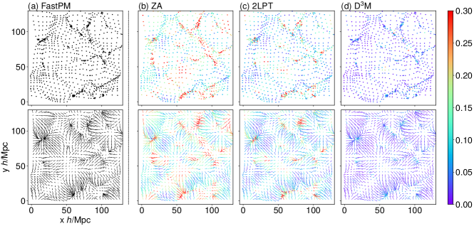
(a) FastPM: the target ground truth, a recent approximate N-body simulation scheme that is based on a particle-mesh (PM) solver ;
(b) Zel’dovich approximation (ZA): a simple linear model that evolves particle along the initial velocity vector;
(c) Second order Lagrangian perturbation theory (2LPT): a commonly used analytical approximatation;
(d) Deep learning model (D3M) as presented in this work.
While FastPM (A) served as our ground truth, B–D include color for the points or vectors. The color indicates the relative difference between the target (a) location or displacement vector and predicted distributions by various methods (b-d). The error-bar shows denser regions have a higher error for all methods. which suggests that it is harder to predict highly non-linear region correctly for all models: D3M, 2LPT and ZA. Our model D3M has smallest differences between predictions and ground truth among the above models (b)-(d).
An important choice in our approach is training with displacement field rather than density field. Displacement field and density field are two ways of describing the same distribution of particles. And an equivalent way to describe density field is the over-density field, defined as , with denoting the mean density. The displacement field and over-density field are related by eq. 1.
| (1) |
When the displacement field is small and has zero curl, the choice of over-density vs displacement field for the output of the model is irrelevant, as there is a bijective map between these two representations, described by the equation:
| (2) |
However as the displacements grow into the non-linear regime of structure formation, different displacement fields can produce identical density fields (e.g. 64). Therefore, providing the model with the target displacement field during the training eliminates the ambiguity associated with the density field. Our inability to produce comparable results when using the density field as our input and target attests that relevant information resides in the displacement field (See SI Appendix, Fig. S1) .
Results and Analysis
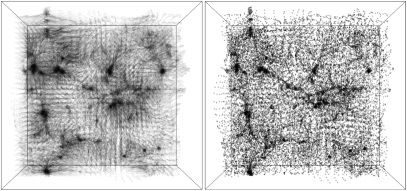
Figure 1 shows the displacement vector field as predicted by D3M (left) and the associated point-cloud representation of the structure formation (right). It is possible to identify structures such as clusters, filaments and voids in this point-cloud representation. We proceed to compare the accuracy of D3M and 2LPT compared with ground truth.
Point-Wise Comparison
Let denote the displacement field, where is the number of spatial resolution elements in each dimension (). A natural measure of error is the relative error , where is the true displacement field (FastPM) and is the prediction from 2LPT or D3M. Figure 2 compares this error for different approximations in a 2-D slice of a single simulation. We observe that D3M predictions are very close to the ground truth, with a maximum relative error of 1.10 over all 1000 simulations. For 2LPT this number is significantly higher at 4.23. In average, the result of D3M comes with a 2.8% relative error while for 2LPT it equals 9.3%.
2-Point Correlation Comparison
As suggested by Figure 2 the denser regions seem to have a higher error for all methods – that is, more non-linearity in structure formation creates larger errors for both D3M and 2LPT. The dependence of error on scale is computed with 2-point and 3-point correlation analysis.
Cosmologists often employ compressed summary statistics of the density field in their studies. The most widely used of these statistics are the 2-point correlation function (2PCF) and its Fourier transform, the power spectrum :
| (3) |
where the ensemble average is taken over all possible realizations of the Universe. Our Universe is observed to be both homogeneous and isotropic on large scales, i.e. without any special location or direction. This allows one to drop the dependencies on and on the direction of , leaving only the amplitude in the final definition of . In the second equation, is simply the Fourier transform of , and captures the dispersion of the plane wave amplitudes at different scales in the Fourier space. is the 3D wavevector of the plane wave, and its amplitude (the wavenumber) is related to the wavelength by . Due to isotropy of the Universe, we drop the vector form of and .
Because FastPM, 2LPT and D3M take the displacement field as input and output, we also study the two-point statistics for the displacement field. The displacement power spectrum is defined as:
| (4) |
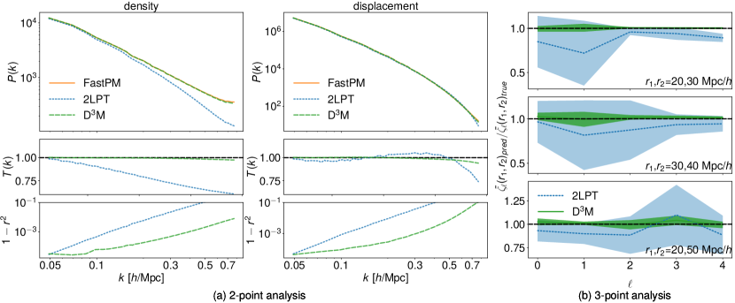
(b) The ratios of the multipole coefficients () (to the target) of the two 3-point correlation functions for several triangle configurations. The results are averaged over 10 test simulations. The error-bars (padded regions) are the standard deviations derived from 10 test simulations. The ratio shows the 3-point correlation function of D3M is closer than 2LPT to our target FastPM with lower variance.
We focus on the Fourier-space representation of the 2-point correlation. Because the matter and the displacement power spectrum take the same form, in what follows we drop the subscript for matter and displacement field and use to stand for both matter and displacement power spectrum. We employ the transfer function and the correlation coefficient as metrics to quantify the model performance against the ground truth (FastPM) in the 2-point correlation. We define the transfer function as the square root of the ratio of two power spectra,
| (5) |
where is the density or displacement power spectrum as predicted by 2LPT or D3M, and analogously is the ground truth predicted by FastPM. The correlation coefficient r(k) is a form of normalized cross power spectrum,
| (6) |
where is the cross power spectrum between 2LPT or D3M predictions and the ground truth (FastPM) simulation result. The transfer function captures the discrepancy between amplitudes, while the correlation coefficient can indicate the discrepancy between phases as functions of scales. For a perfectly accurate prediction, and are both 1. In particular, describes stochasticity, the fraction of the variance in the prediction that cannot be explained by the true model.
Figures 3(a) shows the average power spectrum, transfer function and stochasticity of the displacement field and the density field over 1000 simulations. The transfer function of density from 2LPT predictions is 2% smaller than that of FastPM on large scales (). This is expected since 2LPT performs accurately on very large scales (). The displacement transfer function of 2LPT increases above 1 at and then drops sharply. The increase of 2LPT displacement transfer function is because 2LPT over-estimates the displacement power at small scales (see, e.g. 65). There is a sharp drop of power near the voxel scale because smoothing over voxel scales in our predictions automatically erases power at scales smaller than the voxel size.
Now we turn to the D3M predictions: both the density and displacement transfer functions of the D3M differ from 1 by a mere 0.4% at scale , and this discrepancy only increases to 2% and 4% for density field and displacement field respectively, as increases to the Nyquist frequency around . The stochasticity hovers at approximately and for most scales. In other words, for both the density and displacement fields the correlation coefficient between the D3M predictions and FastPM simulations, all the way down to small scales of is greater than 90%. The transfer function and correlation coefficient of the D3M predictions shows that it can reproduce the structure formation of the Universe from large to semi-non-linear scales. D3M significantly outperforms our benchmark model 2LPT in the 2 point function analysis. D3M only starts to deviate from the ground truth at fairly small scales. This is not surprising as the deeply nonlinear evolution at these scales is more difficult to simulate accurately and appears to be intractable by current analytical theories(66).
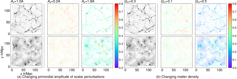
(a) The errorbar shows the difference of particle distribution (upper panel) and displacement fields (lower panel) between and the two extremes for (Center) and (Right).
(b) A similar comparison showing the difference of the particle distributions (upper panel) and displacement fields (lower panel) for smaller and larger values of with regard to , which was used for training.
While the difference for smaller value of () is larger, the displacement for larger () is more non-linear. This non-linearity is due to concentration of mass and makes the prediction more difficult.
3-Point Correlation Comparison
The 3-point correlation function (3PCF) expresses the correlation of the field of interest among 3 locations in the configuration space, which is equivalently defined as bispectrum in Fourier space. Here we concentrate on the 3PCF for computational convenience:
| (7) |
where = and =. Translation invariance guarantees that is independent of . Rotational symmetry further eliminates all direction dependence except dependence on , the angle between and . The multipole moments of , where is the Legendre polynomial of degree , can be efficiently estimated with pair counting (67). While the input (computed by ZA) do not contain significant correlations beyond the second order (power spectrum level), we expect D3M to generate densities with a 3PCF that mimics that of ground truth.
We compare the 3PCF calculated from FastPM, 2LPT and D3M by analyzing the 3PCF through its multipole moments . Figure 3(b) shows the ratio of the binned multipole coefficients of the two 3PCF for several triangle configurations, , where can be the 3PCF for D3M or 2LPT and is the 3PCF for FastPM. We used 10 radial bins with . The results are averaged over 10 test simulations and the errorbars are the standard deviation. The ratio shows the 3PCF of D3M is more close to FastPM than 2LPT with smaller errorbars. To further quantify our comparison, we calculate the relative 3PCF residual defined by
| 3PCF relative residual | |||
| (8) |
where is the number of (,) bins. The mean relative 3PCF residual of the D3M and 2LPT predictions compared to FastPM are and respectively. The D3M accuracy on 3PCF is also an order of magnitude better than 2LPT, which indicates that the D3M is far better at capturing the non-Gaussian structure formation.
Generalizing to New Cosmological Parameters
So far, we train our model using a “single” choice of cosmological parameters (hereafter and (68). is the primordial amplitude of the scalar perturbation from cosmic inflation, and is the fraction of the total energy density that is matter at the present time, and we will call it matter density parameter for short. The true exact value of these parameters are unknown and different choices of these parameters change the large-scale structure of the Universe; see Figure 4.
Here, we report an interesting observation: the D3M trained on a single set of parameters in conjunction with ZA (which depends on and ) as input, can predict the structure formation for widely different choices of and . From a computational point of view this suggests a possibility of producing simulations for a diverse range of parameters, with minimal training data.
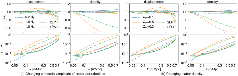
Varying Primordial Amplitude of Scalar Perturbations
After training the D3M using , we change in the input of our test set by nearly one order of magnitude: and . Again, we use 1000 simulations for analysis of each test case. The average relative displacement error of D3M remains less than per voxel (compared to when train and test data have the same parameters). This is still well below the error for 2LPT, which has relative errors of and for larger and smaller values of respectively.
Figure 5(a) shows the transfer function and correlation coefficient for both D3M and 2LPT. The D3M performs much better than 2LPT for . For small , 2LPT does a better job than D3M predicting the density transfer function and correlation coefficient at the largest scales, otherwise D3M predictions are more accurate than 2LPT at scales larger than . We observe a similar trend with 3PCF analysis: the 3PCF of D3M predictions are notably better than 2LPT ones for larger , compared to smaller where it is only slightly better. These results confirm our expectation that increasing increases the non-linearity of the structure formation process. While 2LPT can predict fairly well in linear regimes, compared to D3M its performance deteriorates with increased non-linearity. It is interesting to note that D3M prediction maintains its advantage despite being trained on data from more linear regimes.
Varying matter density parameter
We repeat the same experiments, this time changing to and , while the model is trained on , which is quite far from both of the test sets. For the relative residual displacement errors of the D3M and 2LPT averaged over 1000 simulations are 3.8% and 15.2% and for they are 2.5% and 4.3%. Figures 5(c)(d) show the two-point statistics for density field predicted using different values of . For , the results show that the D3M outperforms 2LPT at all scales, while for smaller , D3M outperforms 2LPT on smaller scales (). As for the 3PCF of simulations with different values of , the mean relative 3PCF residual of the D3M for and are 1.7% and 1.2% respectively and for 2LPT they are 7.6% and 1.7% respectively. The D3M prediction performs better at than . This is again because the Universe is much more non-linear at than . The D3M learns more non-linearity than is encoded in the formalism of 2LPT.
| type | point-wise | † | 3PCF | |||
|---|---|---|---|---|---|---|
| test phase | ||||||
| 2 LPT Density | N/A | 0.96 | 1.00 | 0.74 | 0.94 | 0.0782 |
| D3M Density | N/A | 1.00 | 1.00 | 0.99 | 1.00 | 0.0079 |
| 2 LPT Displacement | 0.093 | 0.96 | 1.00 | 1.04 | 0.90 | N/A |
| D3M Displacement | 0.028 | 1.00 | 1.00 | 0.99 | 1.00 | N/A |
| 2LPT Density | N/A | 0.93 | 1.00 | 0.49 | 0.78 | 0.243 |
| D3M Density | N/A | 1.00 | 1.00 | 0.98 | 1.00 | 0.039 |
| 2LPT Displacement | 0.155 | 0.97 | 1.00 | 1.07 | 0.73 | N/A |
| D3M Displacement | 0.039 | 1.00 | 1.00 | 0.97 | 0.99 | N/A |
| 2LPT Density | N/A | 0.99 | 1.00 | 0.98 | 0.99 | 0.024 |
| D3M Density | N/A | 1.00 | 1.00 | 1.03 | 1.00 | 0.022 |
| 2LPT Displacement | 0.063 | 0.99 | 1.00 | 0.95 | 0.98 | N/A |
| D3M Displacement | 0.036 | 1.00 | 1.00 | 1.01 | 1.00 | N/A |
| 2LPT Density | N/A | 0.94 | 1.00 | 0.58 | 0.87 | 0.076 |
| D3M Density | N/A | 1.00 | 1.00 | 1.00 | 1.00 | 0.017 |
| 2LPT Displacement | 0.152 | 0.97 | 1.00 | 1.10 | 0.80 | N/A |
| D3M Displacement | 0.038 | 1.00 | 1.00 | 0.98 | 0.99 | N/A |
| 2LPT Density | N/A | 0.97 | 1.00 | 0.96 | 0.99 | 0.017 |
| D3M Density | N/A | 0.99 | 1.00 | 1.04 | 1.00 | 0.012 |
| 2LPT Displacement | 0.043 | 0.97 | 1.00 | 0.97 | 0.98 | N/A |
| D3M Displacement | 0.025 | 0.99 | 1.00 | 1.02 | 1.00 | N/A |
†The unit of is . N/A, not applicable
Conclusions
To summarize, our deep model D3M can accurately predict the large-scale structure of the Universe as represented by FastPM simulations, at all scales as seen in the summary table in Table. 1. Furthermore, D3M learns to predict cosmic structure in the non-linear regime more accurately than our benchmark model 2LPT. Finally, our model generalizes well to test simulations with cosmological parameters ( and ) significantly different from the training set. This suggests that our deep learning model can potentially be deployed for a ranges of simulations beyond the parameter space covered by the training data (Table 1). Our results demonstrate that the D3M successfully learns the nonlinear mapping from first order perturbation theory to FastPM simulation beyond what higher order perturbation theories currently achieve.
Looking forward, we expect replacing FastPM with exact N-body simulations would improve the performance of our method. As the complexity of our D3M model is linear in the number of voxels, we expect to be able to further improve our results if we replace the FastPM simulations with higher resolution simulations. Our work suggests that deep learning is a practical and accurate alternative to the traditional way of generating approximate simulations of the structure formation of the Universe.
Materials and Methods
Dataset
The full simulation data consists of 10,000 simulations of boxes with ZA and FastPM as input-output pairs, with an effective volume of 20 (Gpc/h)3 (ly3), comparable to the volume of a large spectroscopic sky survey like Dark Energy Spectroscopic Instrument or EUCLID. We split the full simulation data set into 80%, 10% and 10% for training, validation and test, respectively. We also generated 1000 simulations for 2LPT for each set of tested cosmological parameters.
Model and Training
The D3M adopts the U-Net architecture (54) with 15 convolution or deconvolution layers and approximately trainable parameters. Our D3M generalizes the standard U-Net architecture to work with three-dimensional data (69, 70, 71). The details of the architecture are described in the following sections and a schematic figure of the architecture is shown in SI Appendix, Figure. S2. In the training phase, we employ the Adam Optimizer (72) with a learning rate of 0.0001, and first and second moment exponential decay rates equal to 0.9 and 0.999, respectively. We use the Mean-Squared Error as the loss function (See Loss Function) and regularization with regularization coefficient 0.0001.
Details of the D3M Architecture
The contracting path follows the typical architecture of a convolution network. It consists of two blocks, each of which consists of two successive convolutions of stride 1 and a down-sampling convolution with stride 2. The convolution layers use 333 filters with a periodic padding of size 1 (see Padding and Periodic Boundary) on both sides of each dimension. Notice that at each of the two down-sampling steps, we double the number of feature channels. At the bottom of the D3M, another two successive convolutions with stride 1 and the same periodic padding as above are applied. The expansive path of our D3M is an inverted version of the contracting path of the network. (It includes two repeated applications of the expansion block, each of which consists of one up-sampling transposed convolution with stride 1/2 and two successive convolution of stride 1. The transposed convolution and the convolution are constructed with 333 filters.)
We take special care in the padding and cropping procedure to preserve the shifting and rotation symmetry in the up-sampling layer in expansive path. Before the transposed convolution we apply a periodic padding of length 1 on the right, down and back sides of the box (padding=(0,1,0,1,0,1) in pytorch), and after the transposed convolution, we discard one column on the left, up and front sides of the box and two columns on the right, down and back sides (crop=(1,2,1,2,1,2)).
A special feature of the D3M is the concatenation procedure, where the up-sampling layer halves the feature channels and then concatenates them with the corresponding feature channels on the contracting path, doubling the number of feature channels.
The expansive building block then follows a 111 convolution without padding, which converts the 64 features to the the final 3-D displacement field. All convolutions in the network except the last one are followed by a rectified linear unit activation and batch normalization (BN).
Padding and Periodic Boundary
It is common to use constant or reflective padding in deep models for image processing. However, these approaches are not suitable for our setting. The physical model we are learning is constructed on a spatial volume with a periodic boundary condition. This is sometimes also referred to as a torus geometry, where the boundaries of the simulation box are topologically connected – that is where is the index of the spatial location, and is the periodicity (size of box). Constant or reflective padding strategies break the connection between the physically nearby points separated across the box, which not only loses information but also introduces noise during the convolution, further aggravated with an increased number of layers.
We find that the periodic padding strategy significantly improves the performance and expedites the convergence of our model, comparing to the same network using a constant padding strategy. This is not surprising, as one expects it is easier to train a model that can explain the data than to train a model that does not.
Loss Function
We train the D3M to minimize the mean square error on particle displacements
| (9) |
where labels the particles and the N is the total number of particles. This loss function is proportional to the integrated squared error, and using a Fourier transform and Parseval’s theorem it can be rewritten as
| (10) |
where is the Lagrangian space position, and its corresponding wavevector. is the transfer function defined in Eq. 5, and is the correlation coefficient defined in Eq. 6, which characterize the similarity between the predicted and the true fields, in amplitude and phase respectively. Eq. 10 shows that our simple loss function jointly captures both of these measures: as and approach 1, the loss function approaches 0.
Data availability
The source code of our implementation is available at https://github.com/siyucosmo/ML-Recon. The code to generate the training data is also available at https://github.com/rainwoodman/fastpm. \showmatmethods
We thank Angus Beane, Peter Braam, Gabriella Contardo, David Hogg, Laurence Levasseur, Pascal Ripoche, Zack Slepian and David Spergel for useful suggestions and comments, Angus Beane for comments on the paper, Nick Carriero for help on Center for Computational Astrophysics (CCA) computing clusters. The work is funded partially by Simons Foundation. The FastPM simulations are generated on the computer cluster Edison at the National Energy Research Scientific Computing Center (NERSC), a U.S. Department of Energy Office of Science User Facility operated under Contract No. DE-AC02-05CH11231. The training of neural network model is performed on the CCA computing facility and the Carnegie Mellon University AutonLab computing facility. The open source software toolkit nbodykit (73) is employed for the clustering analysis. YL acknowledges support from the Berkeley Center for Cosmological Physics and the Kavli Institute for the Physics and Mathematics of the Universe, established by World Premier International Research Center Initiative (WPI) of the MEXT, Japan. S.Ho thanks NASA for their support in grant number: NASA grant 15-WFIRST15-0008 and NASA Research Opportunities in Space and Earth Sciences grant 12-EUCLID12-0004, and Simons Foundation.
References
References
- (1) Colless, M., , et al. (2001) The 2dF Galaxy Redshift Survey: Spectra and redshifts. Mon. Not. Roy. Astron. Soc. 328:1039.
- (2) Eisenstein, D.J., , et al. (2011) SDSS-III: Massive Spectroscopic Surveys of the Distant Universe, the Milky Way Galaxy, and Extra-Solar Planetary Systems. Astron. J. 142:72.
- (3) Jones, H.D., , et al. (2009) The 6dF Galaxy Survey: Final Redshift Release (DR3) and Southern Large-Scale Structures. Mon. Not. Roy. Astron. Soc. 399:683.
- (4) Liske, J., , et al. (2015) Galaxy and mass assembly (gama): end of survey report and data release 2. Monthly Notices of the Royal Astronomical Society 452(2):2087.
- (5) Scodeggio, M., , et al. (2016) The VIMOS Public Extragalactic Redshift Survey (VIPERS). Full spectroscopic data and auxiliary information release (PDR-2). ArXiv e-prints.
- (6) Ivezić Ž, et al. (2008) LSST: from Science Drivers to Reference Design and Anticipated Data Products. ArXiv e-prints.
- (7) Amendola L, et al. (2018) Cosmology and fundamental physics with the Euclid satellite. Living Reviews in Relativity 21:2.
- (8) Spergel D, et al. (2015) Wide-Field InfrarRed Survey Telescope-Astrophysics Focused Telescope Assets WFIRST-AFTA 2015 Report. ArXiv e-prints.
- (9) MacFarland T, Couchman HMP, Pearce FR, Pichlmeier J (1998) A new parallel P3M code for very large-scale cosmological simulations. New Astronomy 3(8):687–705.
- (10) Springel V, Yoshida N, White SDM (2001) GADGET: a code for collisionless and gasdynamical cosmological simulations. New Astronomy 6(2):79–117.
- (11) Bagla JS (2002) TreePM: A Code for Cosmological N-Body Simulations. Journal of Astrophysics and Astronomy 23:185–196.
- (12) Bond JR, Kofman L, Pogosyan D (1996) How filaments of galaxies are woven into the cosmic web. Nature 380:603–606.
- (13) Davis M, Efstathiou G, Frenk CS, White SDM (1985) The evolution of large-scale structure in a universe dominated by cold dark matter. ApJ 292:371–394.
- (14) LeCun Y, Bengio Y, Hinton G (2015) Deep learning. nature 521(7553):436.
- (15) Huang G, Liu Z, Van Der Maaten L, Weinberger KQ (2017) Densely connected convolutional networks. in CVPR. Vol. 1, p. 3.
- (16) Karras T, Aila T, Laine S, Lehtinen J (2017) Progressive growing of gans for improved quality, stability, and variation. arXiv preprint arXiv:1710.10196.
- (17) Gulrajani I, Ahmed F, Arjovsky M, Dumoulin V, Courville AC (2017) Improved training of wasserstein gans in Advances in Neural Information Processing Systems. pp. 5767–5777.
- (18) Van Den Oord A, et al. (2016) Wavenet: A generative model for raw audio. CoRR abs/1609.03499.
- (19) Amodei D, et al. (2016) Deep speech 2: End-to-end speech recognition in english and mandarin in International Conference on Machine Learning. pp. 173–182.
- (20) Hu Z, Yang Z, Liang X, Salakhutdinov R, Xing EP (2017) Toward controlled generation of text. arXiv preprint arXiv:1703.00955.
- (21) Vaswani A, et al. (2017) Attention is all you need in Advances in Neural Information Processing Systems. pp. 5998–6008.
- (22) Denton E, Fergus R (2018) Stochastic video generation with a learned prior. arXiv preprint arXiv:1802.07687.
- (23) Donahue J, et al. (2015) Long-term recurrent convolutional networks for visual recognition and description in Proceedings of the IEEE conference on computer vision and pattern recognition. pp. 2625–2634.
- (24) Silver D, et al. (2016) Mastering the game of go with deep neural networks and tree search. nature 529(7587):484.
- (25) Mnih V, et al. (2015) Human-level control through deep reinforcement learning. Nature 518(7540):529.
- (26) Levine S, Finn C, Darrell T, Abbeel P (2016) End-to-end training of deep visuomotor policies. The Journal of Machine Learning Research 17(1):1334–1373.
- (27) Ching T, et al. (2018) Opportunities and obstacles for deep learning in biology and medicine. Journal of The Royal Society Interface 15(141):20170387.
- (28) Alipanahi B, Delong A, Weirauch MT, Frey BJ (2015) Predicting the sequence specificities of dna-and rna-binding proteins by deep learning. Nature biotechnology 33(8):831.
- (29) Segler MH, Preuss M, Waller MP (2018) Planning chemical syntheses with deep neural networks and symbolic ai. Nature 555(7698):604.
- (30) Gilmer J, Schoenholz SS, Riley PF, Vinyals O, Dahl GE (2017) Neural message passing for quantum chemistry. arXiv preprint arXiv:1704.01212.
- (31) Carleo G, Troyer M (2017) Solving the quantum many-body problem with artificial neural networks. Science 355(6325):602–606.
- (32) Adam-Bourdarios C, et al. (2015) The higgs boson machine learning challenge in NIPS 2014 Workshop on High-energy Physics and Machine Learning. pp. 19–55.
- (33) He S, Ravanbakhsh S, Ho S (2018) Analysis of Cosmic Microwave Background with Deep Learning. International Conference on Learning Representations Workshop.
- (34) Perraudin N, Defferrard M, Kacprzak T, Sgier R (2018) Deepsphere: Efficient spherical convolutional neural network with healpix sampling for cosmological applications. arXiv preprint arXiv:1810.12186.
- (35) Caldeira J, et al. (2018) Deepcmb: Lensing reconstruction of the cosmic microwave background with deep neural networks. arXiv preprint arXiv:1810.01483.
- (36) Ravanbakhsh, S., et al. (2017) Estimating cosmological parameters from the dark matter distribution. ArXiv e-prints.
- (37) Mathuriya A, et al. (2018) Cosmoflow: using deep learning to learn the universe at scale. arXiv preprint arXiv:1808.04728.
- (38) Hezaveh, Y. D., Levasseur, L. P., Marshall, P. J. (2017) Fast automated analysis of strong gravitational lenses with convolutional neural networks. Nature 548:555-557.
- (39) Lanusse, F., et al. (2018) Cmu deeplens: deep learning for automatic image-based galaxy-galaxy strong lens finding. MNRAS pp. 3895–3906.
- (40) Kennamer N, Kirkby D, Ihler A, Sanchez-Lopez FJ (2018) ContextNet: Deep learning for star galaxy classification in Proceedings of the 35th International Conference on Machine Learning, Proceedings of Machine Learning Research. Vol. 80, pp. 2582–2590.
- (41) Kim EJ, Brunner RJ (2016) Star-galaxy classification using deep convolutional neural networks. Monthly Notices of the Royal Astronomical Society p. stw2672.
- (42) Lochner M, McEwen JD, Peiris HV, Lahav O, Winter MK (2016) Photometric supernova classification with machine learning. The Astrophysical Journal Supplement Series 225(2):31.
- (43) Battaglia PW, Hamrick JB, Tenenbaum JB (2013) Simulation as an engine of physical scene understanding. Proceedings of the National Academy of Sciences p. 201306572.
- (44) Battaglia P, Pascanu R, Lai M, Rezende DJ, , et al. (2016) Interaction networks for learning about objects, relations and physics in Advances in neural information processing systems. pp. 4502–4510.
- (45) Mottaghi R, Bagherinezhad H, Rastegari M, Farhadi A (2016) Newtonian scene understanding: Unfolding the dynamics of objects in static images in Proceedings of the IEEE Conference on Computer Vision and Pattern Recognition. pp. 3521–3529.
- (46) Chang MB, Ullman T, Torralba A, Tenenbaum JB (2016) A compositional object-based approach to learning physical dynamics. arXiv preprint arXiv:1612.00341.
- (47) Wu J, Yildirim I, Lim JJ, Freeman B, Tenenbaum J (2015) Galileo: Perceiving physical object properties by integrating a physics engine with deep learning in Advances in neural information processing systems. pp. 127–135.
- (48) Wu J, Lim JJ, Zhang H, Tenenbaum JB, Freeman WT (2016) Physics 101: Learning physical object properties from unlabeled videos. in BMVC. Vol. 2, p. 7.
- (49) Watters N, et al. (2017) Visual interaction networks: Learning a physics simulator from video in Advances in Neural Information Processing Systems. pp. 4539–4547.
- (50) Lerer A, Gross S, Fergus R (2016) Learning physical intuition of block towers by example. arXiv preprint arXiv:1603.01312.
- (51) Agrawal P, Nair AV, Abbeel P, Malik J, Levine S (2016) Learning to poke by poking: Experiential learning of intuitive physics in Advances in Neural Information Processing Systems. pp. 5074–5082.
- (52) Fragkiadaki K, Agrawal P, Levine S, Malik J (2015) Learning visual predictive models of physics for playing billiards. arXiv preprint arXiv:1511.07404.
- (53) Tompson J, Schlachter K, Sprechmann P, Perlin K (2016) Accelerating eulerian fluid simulation with convolutional networks. arXiv preprint arXiv:1607.03597.
- (54) Ronneberger, O.; Fischer P, Brox T (2015) U-Net: Convolutional Networks for Biomedical Image Segmentation. Medical Image Computing and Computer-Assisted Intervention – MICCAI 2015 9351:234–241.
- (55) Zel’dovich YB (1970) Gravitational instability: An approximate theory for large density perturbations. A&A 5:84–89.
- (56) White M (2014) The Zel’dovich approximation. MNRAS 439:3630–3640.
- (57) Feng Y, Chu MY, Seljak U, McDonald P (2016) FASTPM: a new scheme for fast simulations of dark matter and haloes. MNRAS 463:2273–2286.
- (58) Buchert T (1994) Lagrangian Theory of Gravitational Instability of Friedman-Lemaitre Cosmologies - a Generic Third-Order Model for Nonlinear Clustering. MNRAS 267:811.
- (59) Jasche J, Wandelt BD (2013) Bayesian physical reconstruction of initial conditions from large-scale structure surveys. MNRAS 432:894–913.
- (60) Kitaura FS (2013) The initial conditions of the Universe from constrained simulations. MNRAS 429:L84–L88.
- (61) Dawson KS, et al. (2013) The Baryon Oscillation Spectroscopic Survey of SDSS-III. AJ 145:10.
- (62) Dawson KS, et al. (2016) The SDSS-IV Extended Baryon Oscillation Spectroscopic Survey: Overview and Early Data. AJ 151:44.
- (63) DESI Collaboration, et al. (2016) The DESI Experiment Part I: Science,Targeting, and Survey Design. ArXiv e-prints.
- (64) Feng Y, Seljak U, Zaldarriaga M (2018) Exploring the posterior surface of the large scale structure reconstruction. J. Cosmology Astropart. Phys 7:043.
- (65) Chan KC (2014) Helmholtz decomposition of the Lagrangian displacement.
- (66) Perko A, Senatore L, Jennings E, Wechsler RH (2016) Biased Tracers in Redshift Space in the EFT of Large-Scale Structure. arXiv e-prints p. arXiv:1610.09321.
- (67) Slepian Z, Eisenstein DJ (2015) Computing the three-point correlation function of galaxies in time.
- (68) Planck Collaboration, et al. (2016) Planck 2015 results. XIII. Cosmological parameters.
- (69) Milletari F, Navab N, Ahmadi SA (2016) V-Net: Fully Convolutional Neural Networks for Volumetric Medical Image Segmentation. ArXiv e-prints.
- (70) Berger P, Stein G (2019) A volumetric deep Convolutional Neural Network for simulation of mock dark matter halo catalogues. MNRAS 482:2861–2871.
- (71) Aragon-Calvo MA (2018) Classifying the Large Scale Structure of the Universe with Deep Neural Networks. ArXiv e-prints.
- (72) Kingma D, Ba J (2014) Adam: A method for stochastic optimization. eprint arXiv: 1412.6980.
- (73) Hand N, et al. (2018) nbodykit: an open-source, massively parallel toolkit for large-scale structure. The Astronomical Journal 156(4):160.