The $q$-Hahn PushTASEP

Abstract

We introduce the $q$-Hahn PushTASEP — an integrable stochastic interacting particle system which is a 3-parameter generalization of the PushTASEP, a well-known close relative of the TASEP (Totally Asymmetric Simple Exclusion Process). The transition probabilities in the $q$-Hahn PushTASEP are expressed through the ${}_{4}\phi_{3}$ basic hypergeometric function. Under suitable limits, the $q$-Hahn PushTASEP degenerates to all known integrable (1+1)-dimensional stochastic systems with a pushing mechanism. One can thus view our new system as a pushing counterpart of the $q$-Hahn TASEP introduced by Povolotsky [Pov13]. We establish Markov duality relations and contour integral formulas for the $q$-Hahn PushTASEP.

In a $q\to 1$ limit of our process we arrive at a random recursion which, in a special case, appears to be similar to the inverse-Beta polymer model. However, unlike in recursions for Beta polymer models, the weights (i.e., the coefficients of the recursion) in our model depend on the previous values of the partition function in a nontrivial manner.

1 Introduction

Integrable probability is a field which seeks to discover and analyze probabilistic systems enjoying significant algebraic structure (e.g. Markov dualities and Bethe ansatz diagonalizability) and which demonstrate universal asymptotic fluctuation behaviors. There are two main routes which have proved effective so far in producing integrable probabilistic systems — Macdonald processes (and various degenerations) [BC14], [BG16], [BP14], and stochastic vertex models [Bor17], [CP16], [BP16].

Prototypical examples within both classes of integrable models are the TASEP (Totally Asymmeric Simple Exclusion Process) [Spi70] and the PushTASEP, its counterpart with a long-range pushing mechanism [Lig80], [DLSS91]. In the context of Macdonald processes, both systems are connected to certain probability distributions on integer partitions $\lambda=(\lambda_{1}\geq\ldots\geq\lambda_{N}\geq 0)$ with nice algebraic structure, and the TASEP and PushTASEP are related to the distributions of, respectively, the smallest and the largest parts of $\lambda$. This picture can be generalized within the Macdonald process hierarchy to produce 2-parameter $q$-deformed discrete and continuous time TASEPs and PushTASEPs [BC15], [BP16a], [CP15], [MP17]. On the other hand, TASEP also belongs to the class of exactly solvable stochastic vertex models, and hence it admits a 3-parameter generalization to the $q$-Hahn TASEP [Pov13], [Cor14] (recalled in Section 2). The latter is, in fact, a special case of the 4-parameter family of stochastic higher spin six vertex models studied in [CP16], [BP16].

For some time it was not clear how to extend the PushTASEP analogously outside the Macdonald hierarchy. In this paper we achieve this. That is, we introduce a 3-parameter $q$-Hahn generalization of the PushTASEP (Section 3.1), adding a new parameter to the $q$-PushTASEP with $q$-geometric jumps discovered in [MP17]. This is akin to the $q$-Hahn extension of the discrete time $q$-TASEP [BC15] found in [Pov13] and studied in [Cor14]. Our pushing system enjoys a variant of Markov duality (see Theorem 3.4) similar to the one studied earlier for the continuous time $q$-PushTASEP [CP15], and generalizes the contour integral formulas from that setting, too (see Theorem 3.10). The system itself is not so simple (in particular, its transition probabilities are expressed through the basic hypergeometric function ${}_{4}\phi_{3}$), and our search for it was informed by the desire to extend the duality and contour integral formulas away from the Macdonald context. Even once this generalized system is introduced (see Section 3.1), it is not so simple to prove the duality, as it requires some interesting $q$-identities (the central statement is Lemma 3.7 which we prove in Section 3.4).

The $q$-Hahn TASEP revealed some interesting new systems as its limits — in particular, the beta polymer (or random walk in random environment) considered in [BC16] which arises in a scaling limit of the system as $q\to 1$. We parallel this limit here, and discover a corresponding beta polymer-like system. The main new feature is that in our model, the distribution of the weights depends on the ratio of the partition functions immediately to the left and below (see Definition 4.1). We had initially expected that the inverse beta polymer of [TLD15] would arise from our pushing system, but presently this does not seem to be the case (though perhaps the inverse beta polymer could be included into a 4-parameter family of pushing systems whose existence we speculate on below). However, in the $q\to 1$ limit we do arrive (see Lemma 4.3 and Theorem 4.4) at a solution to the following recursion relation, which bears great similarity to that satisfied by the inverse beta polymer: When $\tilde{Z}(i,t-1)>\tilde{Z}(i-1,t)$,

$$\tilde{Z}(i,t)=\tilde{Y}\tilde{Z}(i,t-1)+(1-\tilde{Y})\tilde{Z}(i-1,t)$$

where $\tilde{Y}$ is $\mathscr{Beta}^{-1}(\bar{\mu},\tfrac{1}{2}-\bar{\mu})$-distributed (see Section A.4); and when $\tilde{Z}(i,t-1)<\tilde{Z}(i-1,t)$,

$$\tilde{Z}(i,t)=\tilde{Y}\tilde{Z}(i-1,t)+(1-\tilde{Y})\tilde{Z}(i,t-1)$$

where $\tilde{Y}$ is $\mathscr{Beta}^{-1}(\bar{\mu},\tfrac{1}{2})$-distributed. For this random recursion (with suitable boundary data) we compute moment formulas (Proposition 4.6) and conjecture a Laplace transform formula (4.7).

Besides the $q\to 1$ limits, there are other new limit processes which arise from our work. In particular, for $q=0$ we find a geometric-Bernoulli generalization of the PushTASEP (see Section 3.2.2).

We do not perform any asymptotics in this paper. In fact, the key result towards such an aim would be a Fredholm determinant formula for a suitable $q$-Laplace transform. However, due to the pushing mechanism, the moments generally used to derive such a formula become infinite past a certain power. Still, we present 3.11 which contains what we believe is a correct formula based on previous analogous works.

Our present investigation suggests that there should be strong parallels between pushing and non-pushing integrable particle systems. In the non-pushing (e.g. standard TASEP) context, [CP16] introduced a 4-parameter family of stochastic vertex models, which recovers the 3-parameter $q$-Hahn TASEP in a special analytic continuation and degeneration. It would be interesting to develop a parallel 4-parameter family of pushing systems, and obtain the corresponding duality relations and contour integral formulas. We expect that this can be done in the following manner. Consider the stochastic higher spin vertex model with horizontal spin $J\in\mathbb{Z}_{\geq 1}$. Subtract $J$ from the number of arrows along each horizontal edge, and interpret the negative arrow numbers as counting arrows pointing in the opposite direction. This minor modification introduces a pushing mechanism. It seems likely that duality and contour integral formulas can be carried over from the original stochastic higher spin model. On the other hand, to recover the $q$-Hahn PushTASEP one must find the right analytic continuation. We leave this for a later investigation.

We also note that it should be possible to produce a 4-parameter family of pushing systems by a different mechanism — via bijectivisation of the Yang-Baxter equation (see [BP17]) related to the spin $q$-Whittaker polynomials (introduced in [BW17]). This approach is developed in the upcoming work [BMP18], and we anticipate that the same 4-parameter family will come up in this manner.

Outline

In Section 2 we recall duality and contour integral formulas for the $q$-moments of the $q$-Hahn TASEP [Pov13], [Cor14], as some of these ingredients are used for the $q$-Hahn PushTASEP. In Section 3 we introduce the $q$-Hahn PushTASEP, discuss its various degenerations, and prove duality and contour integral formulas. In Section 4 we consider a beta polymer-like limit of the $q$-Hahn PushTASEP as $q\to 1$, and write down moments of the resulting system in a contour integral form. We also provide a conjecture for the $q$-Laplace transform. Formulas pertaining to $q$-hypergeometric functions and associated probability distributions on $\mathbb{Z}$ are summarized in Appendix A.

Acknowledgments

The authors thank Guillaume Barraquand for pointing out the simplification which led to Section 4.2. The authors acknowledge that part of this work was done while in attendance of the ICERM conference on Limit Shapes, held from April 13-17, 2015. IC was partially supported by the NSF grants DMS-1208998, DMS-1811143 and DMS-1664650, as well as a Packard Fellowship in Science and Engineering and a Clay Research Fellowship. LP was partially supported by the NSF grant DMS-1664617.

2 $q$-Hahn TASEP

Here we briefly recall the definition and duality properties of the $q$-Hahn TASEP introduced and studied in [Pov13], [Cor14].

Assume that the parameters $0<q<1$, $0\leq\boldsymbol{\upnu}\leq\boldsymbol{\upmu}<1$ are fixed. The $q$-Hahn TASEP is a discrete time (with $t\in\mathbb{Z}_{\geq 0}$) Markov process on configurations $\vec{x}(t)=(x_{1}(t)>x_{2}(t)>\ldots)$, $x_{i}\in\mathbb{Z}$, with at most one particle per site and a rightmost particle $x_{1}$. The evolution of the $q$-Hahn TASEP is as follows. At each discrete time step $t\to t+1$, each particle $x_{i}(t)$ jumps in parallel and independently to $x_{i}(t+1)=x_{i}(t)+v_{i}$, where $v_{i}$ is sampled from the probability distribution $\varphi_{q,\boldsymbol{\upmu},\boldsymbol{\upnu}}(v_{i}\mid x_{i-1}(t)-x_{i}(t)-1)$. Note for the update of $x_{1}$, we assume a virtual particle $x_{0}\equiv+\infty$, by agreement. Here $\varphi_{q,\boldsymbol{\upmu},\boldsymbol{\upnu}}$ is the $q$-beta-binomial distribution defined by (A.2). See Figure 1 for an illustration.

Figure 1: $q$-Hahn TASEP and the update probabilities $\varphi_{q,\boldsymbol{\upmu},\boldsymbol{\upnu}}$ for $x_{1}$ and $x_{2}$.

We now proceed to describe a Markov duality relation between the $q$-Hahn TASEP one-step transition operator and the $q$-Hahn Boson operator on a different space. Fix $N\geq 1$ and define the $N$-particle space

$$\mathbb{X}^{N}:=\{\vec{x}:=(x_{0},x_{1},\ldots,x_{N}),\ x_{i}\in\mathbb{Z},\ +\infty=x_{0}>x_{1}>\ldots>x_{N}\}.$$ (2.1)

By $\mathsf{P}^{\textnormal{TASEP}}_{q,\boldsymbol{\upmu},\boldsymbol{\upnu}}$ denote the $q$-Hahn TASEP Markov transition operator acting on functions on $\mathbb{X}^{N}$. Note that by the very definition of the $q$-Hahn TASEP, the evolution of its $N$ rightmost particles is independent from the rest of the process.

Also define the Boson particle spaces

$$\mathbb{Y}^{N}:=\{\vec{y}=(y_{0},y_{1},\ldots,y_{N})\in\mathbb{Z}_{\geq 0}^{N+1}\},\qquad\mathbb{Y}^{N}_{k}:=\{\vec{y}\in\mathbb{Y}^{N}\colon y_{0}+y_{1}+\ldots+y_{N}=k\}.$$ (2.2)

Let us define the $q$-Hahn Boson operator $\mathsf{P}^{\textnormal{Boson}}_{q,\alpha,\boldsymbol{\upnu}}$ acting on functions on $\mathbb{Y}^{N}$, where the parameter $\alpha$ is arbitrary. First, let $[\mathcal{A}_{q,\alpha,\boldsymbol{\upnu}}]_{i}$, $i=1,\ldots,N$, be a local operator acting only on the $y_{i}$ and $y_{i-1}$ coordinates of functions $f$ as

$$[\mathcal{A}_{q,\alpha,\boldsymbol{\upnu}}]_{i}f(\vec{y})=\sum_{s_{i}=0}^{y_{i}}\varphi_{q,\alpha,\boldsymbol{\upnu}}(s_{i}\mid y_{i})\,f(y_{0},y_{1},\ldots,y_{i-1}+s_{i},y_{i}-s_{i},\ldots,y_{N}).$$

Define the $q$-Hahn Boson operator by its action

$$\mathsf{P}^{\textnormal{Boson}}_{q,\alpha,\boldsymbol{\upnu}}f(\vec{y}):=[\mathcal{A}_{q,\alpha,\boldsymbol{\upnu}}]_{N}\ldots[\mathcal{A}_{q,\alpha,\boldsymbol{\upnu}}]_{1}f(\vec{y}).$$

The order of operators is important and corresponds to parallel update: first move particles from location 1 to location 0, then from location 2 to location 1 (note that the distribution of the particles taken from location 2 is no affected by what happened at location 1), and so on. No particles are moved from the location $0$, and no particles are added to the location $N$. This implies that $\mathsf{P}^{\textnormal{Boson}}_{q,\alpha,\boldsymbol{\upnu}}$ preserves each of the spaces $\mathbb{Y}^{N}_{k}$.

Remark 2.1.

We put no restrictions on the parameter $\alpha$ in $\mathsf{P}^{\textnormal{Boson}}_{q,\alpha,\boldsymbol{\upnu}}$. In particular, we do not require it to be a Markov transition operator: it is allowed to have negative matrix elements. However, the rows in $\mathsf{P}^{\textnormal{Boson}}_{q,\alpha,\boldsymbol{\upnu}}$ still sum to one, and for $\boldsymbol{\upnu}\leq\alpha<1$ the operator $\mathsf{P}^{\textnormal{Boson}}_{q,\alpha,\boldsymbol{\upnu}}$ defines a discrete time Markov process on $\mathbb{Y}^{N}$ called the $q$-Hahn Boson system.

The $q$-Hahn TASEP and $q$-Hahn Boson operators with the same parameters $\alpha=\boldsymbol{\upmu}$ are dual to each other via the duality functional $\mathfrak{H}\colon\mathbb{X}^{N}\times\mathbb{Y}^{N}\to\mathbb{R}$ defined as

$$\mathfrak{H}(\vec{x},\vec{y}):=\begin{cases}\displaystyle\prod_{i=1}^{N}q^{y_{i}(x_{i}+i)},&y_{0}=0;\\[10.0pt] 0,&y_{0}>0.\end{cases}$$ (2.3)

Theorem 2.2 (Duality for the $q$-Hahn TASEP [Cor14]).

We have

$$\mathsf{P}^{\textnormal{TASEP}}_{q,\boldsymbol{\upmu},\boldsymbol{\upnu}}\mathfrak{H}=\mathfrak{H}\bigl{(}\mathsf{P}^{\textnormal{Boson}}_{q,\boldsymbol{\upmu},\boldsymbol{\upnu}}\bigr{)}^{T},$$

where “$T$” stands for transpose of an operator. In other words, $\mathsf{P}^{\textnormal{TASEP}}_{q,\boldsymbol{\upmu},\boldsymbol{\upnu}}$ acts in the variables $\vec{x}$, and $\mathsf{P}^{\textnormal{Boson}}_{q,\boldsymbol{\upmu},\boldsymbol{\upnu}}$ acts in the variables $\vec{y}$, and their actions on $\mathfrak{H}(\vec{x},\vec{y})$ coincide.

An immediate consequence of the duality is that the $q$-moments $\mathop{\mathbb{E}}\bigl{[}\prod_{i=1}^{n}q^{y_{i}(x_{i}(t)+i)}\bigr{]}$ of the $q$-Hahn TASEP, as index by time $t$ and the vector $\vec{y}$ solves a difference equation involving the $q$-Hahn Boson operator. Using the Bethe ansatz solvability of this Boson operator allows one to write down explicit contour integral formulas for the $q$-moments, which become particularly nice when the $q$-Hahn TASEP is started from the step [Cor14] or the half-stationary [BCPS15] initial data.

Let us recall the formulas in the step case. Encode elements of $\mathbb{Y}^{N}_{k}$ as $\vec{n}=(n_{1}\geq\ldots\geq n_{k})$, $N\geq n_{1}$, $n_{k}\geq 0$, where for all $m$ we have $y_{m}=\#\{i\colon n_{i}=m\}$.

Theorem 2.3 ([Cor14, Theorem 1.9]).

Fix $0<q<1$, $0\leq\boldsymbol{\upnu}\leq\boldsymbol{\upmu}<1$. For any $N,k\geq 1$ and $\vec{n}$ as above, the $q$-moments of the $q$-Hahn PushTASEP with step initial data $x_{i}(0)=-i$, $i\geq 1$, have the form

$$\mathop{\mathbb{E}}\Bigl{[}\prod_{i=1}^{k}q^{x_{n_{i}}(t)+n_{i}}\Bigr{]}=\frac{(-1)^{k}q^{\frac{k(k-1)}{2}}}{(2\pi\sqrt{-1})^{k}}\oint\frac{dz_{1}}{z_{1}}\ldots\oint\frac{dz_{k}}{z_{k}}\prod_{1\leq A<B\leq k}\frac{z_{A}-z_{B}}{z_{A}-qz_{B}}\\ \times\prod_{i=1}^{k}\Biggl{[}\left(\frac{1-\boldsymbol{\upnu}z_{j}}{1-z_{j}}\right)^{n_{j}}\left(\frac{1-\boldsymbol{\upmu}z_{j}}{1-\boldsymbol{\upnu}z_{j}}\right)^{t}\frac{1}{1-\boldsymbol{\upnu}z_{j}}\Biggr{]}.$$

Here all the integration contours encircle $1$ but not $0$ or $\boldsymbol{\upnu}^{-1}$, and for all $B>A$ the $z_{A}$ contour encircles the $qz_{B}$ contour.

The parameters $y_{i}$ are the labels of the $q$-moments. In Section 3.3 we prove a duality result for the $q$-Hahn PushTASEP, and in Section 3.5 utilize the duality to obtain contour integral formulas for the $q$-moments of this process.

3 $q$-Hahn PushTASEP, duality, and contour integrals

3.1 Definition and nonnegativity

The $q$-Hahn PushTASEP depends on the main “quantization” parameter $q\in(0,1)$, and on two parameters $\mu,\nu$ in the following range:

$$0<\mu<1,\qquad-1<\nu\leq\min\{\mu,\sqrt{q}\}.$$ (3.1)

The $q$-Hahn PushTASEP is a discrete time Markov process on particle configurations in $\mathbb{Z}$ (with at most one particle per site) which have a rightmost particle:

$$\vec{x}(t)=(x_{1}(t)>x_{2}(t)>\ldots).$$

At each discrete time moment, particles in the $q$-Hahn PushTASEP may jump to the left. The update $\vec{x}(t)\to\vec{x}(t+1)$ is performed according to the following procedure (the distributions $\varphi$ and $\psi$ are defined by (A.2) and (A.7), respectively):

1. The first particle $x_{1}$ jumps to the left by $\ell\in\mathbb{Z}_{\geq 0}$, where $\ell$ is drawn from the distribution $\varphi_{q,\mu,\nu}(\ell\mid\infty)$.

2. Consecutively for $i=2,3,\ldots$, given the movement of the $(i-1)$-st particle $x_{i-1}(t)\to x_{i-1}(t+1)=x_{i-1}(t)-\ell$, and the gap $g=x_{i-1}(t)-x_{i}(t)-1$ before this movement, the location of the $i$-th particle is updated as $x_{i}(t)\to x_{i}(t+1)=x_{i}(t)-L$, $L\in\mathbb{Z}_{\geq 0}$, with probability

   $$\mathbf{P}_{\ell,g}(L):=\sum_{p=0}^{\min\{\ell,L\}}\varphi_{q^{-1},q^{g},\mu\nu q^{g-1}}(p\mid\ell)\,\psi_{q,\nu\mu^{-1}q^{p},\nu q^{g},\nu^{2}q^{g+p}}(L-p).$$ (3.2)

   For consistency of notation we will sometimes write $x_{0}=+\infty$ and $\mathbf{P}_{\ell,\infty}(L)=\varphi_{q,\mu,\nu}(L\mid\infty)$. See Figure 2 for an illustration.

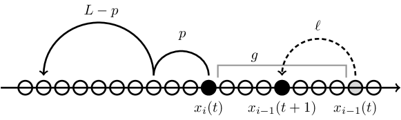
Figure 2: Update of the $i$-th particle given the movement of the $(i-1)$-st particle.

Let us make a number of comments concerning this definition:

1. It is not obvious that the right-hand side of (3.2) is nonnegative because for $\nu>0$ the expression $\varphi_{q^{-1},q^{g},\mu\nu q^{g-1}}(p\mid\ell)$ might be negative. We prove the nonnegativity of the $\mathbf{P}_{\ell,g}$’s in Proposition 3.1 below.

2. The update probabilities $\mathbf{P}_{\ell,g}$ are given by a complicated expression involving $q$-Pochhammer symbols. In Section 3.2 below we discuss a number of previously studied PushTASEP like processes which arise as degenerations of the $q$-Hahn PushTASEP. In particular, under these degenerations the $\mathbf{P}_{\ell,g}$’s simplify.

3. One can check that $\mathbf{P}_{\ell,g}(L)=0$ unless $L\geq\ell-g$. (Indeed, this is because $\varphi_{q^{-1},q^{g},\mu\nu q^{g-1}}(p\mid\ell)=0$ unless $\ell-p\leq g$.) In words, if the previous jumping distance $\ell$ is greater than the gap between $x_{i-1}$ and $x_{i}$, then the particle $x_{i}$ is deterministically pushed to the left. Therefore, update rule (3.2) preserves the order of the particles.

4. If $\ell>g$ and $\mu\nu$ equals $q^{y}$ for a positive integer $y$, the denominator in $\varphi_{q^{-1},q^{g},\mu\nu q^{g-1}}(p\mid\ell)$ (A.2) may vanish. However, we can still define $\varphi$ by continuity (canceling the corresponding factor in the numerator).

5. The process can make infinitely many jumps in a single discrete time step (for example, when it starts from the step initial configuration $x_{i}(0)=-i$, $i\geq 0$). However, for each $N$ the behavior of the particles $x_{i}$, $i\leq N$, is independent from the one of with $i>N$. Therefore, the dynamics restricted to $x_{1},\ldots,x_{N}$ is well-defined as a process with finitely many particles. These $N$-particle dynamics are compatible for various $N$, and so the dynamics of the process on infinite particle configurations having a rightmost particle is well-defined.

Proposition 3.1.

Under the restrictions (3.1) on parameters we have $\mathbf{P}_{\ell,g}(L)\geq 0$ for all $\ell,g,L\in\mathbb{Z}_{\geq 0}$, and $\sum_{L\in\mathbb{Z}_{\geq 0}}\mathbf{P}_{\ell,g}(L)=1$.

Proof.

The fact that $\sum_{L\in\mathbb{Z}_{\geq 0}}\mathbf{P}_{\ell,g}(L)=1$ follows by interchanging the summations over $L$ and $p$ (the latter coming from (3.2)) and using

$$\sum_{p=0}^{\ell}\varphi_{q^{-1},q^{g},\mu\nu q^{g-1}}(p\mid\ell)=1,\qquad\sum_{L=p}^{\infty}\psi_{q,\nu\mu^{-1}q^{p},\nu q^{g},\nu^{2}q^{g+p}}(L-p)=1,$$

see Appendix A.

Turning to proving the positivity, there are two cases depending on the sign of $\nu$. First, we have $\varphi_{q^{-1},q^{g},\mu\nu q^{g-1}}(p\mid\ell)\geq 0$ when $-1<\nu\leq 0$. Therefore, we can think that the $i$-th particle first moves $x_{i}(t)\to x_{i}(t)-p$ with probability $\varphi_{q^{-1},q^{g},\mu\nu q^{g-1}}(p\mid\ell)$ due to the push of the $i-1$-st particle. After that, the $i$-th particle makes an extra move $x_{i}(t)-p\to x_{i}(t)-p-m$ (where $m+p=L$) with probability $\psi_{q,\nu\mu^{-1}q^{p},\nu q^{g},\nu^{2}q^{g+p}}(m)\geq 0$. In other words, the jump by $L$ in Figure 2 is a combination of two jumps, by $p$ and $L-p$ (with $p$ random), each happening with a nonnegative probability.

In the second case $0<\nu\leq\min\{\mu,\sqrt{q}\}$ the expression $\varphi_{q^{-1},q^{g},\mu\nu q^{g-1}}(p\mid\ell)$ might become negative, and the previous interpretation does not imply nonnegativity of $\mathbf{P}_{\ell,g}(L)$. Let us rewrite $\mathbf{P}_{\ell,g}(L)$ in two different ways (depending on the order of $\ell$ and $g$) to show the nonnegativity. We have (here and below in the proof we use the notation from Section A.1)

$$\mathbf{P}_{\ell,g}(L) =\sum_{p=0}^{\min\{\ell,L\}}q^{gp}\frac{(\mu\nu/q;q^{-1})_{p}(q^{g};q^{-1})_{\ell-p}}{(\mu\nu q^{g-1};q^{-1})_{\ell}}\frac{(q^{-1};q^{-1})_{\ell}}{(q^{-1};q^{-1})_{p}(q^{-1};q^{-1})_{\ell-p}}$$

$$\hskip 100.0pt\times\mu^{L-p}\frac{(\nu\mu^{-1}q^{p},\nu q^{g};q)_{L-p}}{(q,\nu^{2}q^{g+p};q)_{L-p}}\frac{(\nu^{2}q^{g+p},\mu;q)_{\infty}}{(\nu q^{p},\mu\nu q^{g};q)_{\infty}}$$

$$=\frac{(\mu;q)_{\infty}(\nu^{2}q^{g};q)_{\infty}}{(\nu;q)_{\infty}(\nu\mu q^{g};q)_{\infty}}\sum_{p=0}^{\min\{\ell,L\}}q^{gp}\frac{(\mu\nu/q;q^{-1})_{p}(q^{g};q^{-1})_{\ell-p}}{(\mu\nu q^{g-1};q^{-1})_{\ell}}\frac{(q^{-1};q^{-1})_{\ell}}{(q^{-1};q^{-1})_{p}(q^{-1};q^{-1})_{\ell-p}}$$ (3.3)

$$\hskip 100.0pt\times\mu^{L-p}\frac{(\nu\mu^{-1}q^{p},\nu q^{g};q)_{L-p}}{(q,\nu^{2}q^{g+p};q)_{L-p}}\frac{(\nu;q)_{p}}{(\nu^{2}q^{g};q)_{p}}.$$

When $\ell<g$, this expression is rewritten as follows:

$$\mathbf{P}_{\ell,g}(L)=\mu^{L}\frac{(q^{g};q^{-1})_{\ell}(\nu\mu^{-1};q)_{L}(\nu q^{g};q)_{L}}{(\mu\nu q^{g-1};q^{-1})_{\ell}(q;q)_{L}(\nu^{2}q^{g};q)_{L}}\\ {{}_{4}}\phi_{3}\left[\begin{array}[]{cccc}q^{-\ell}&\mu^{-1}\nu^{-1}q&\nu&q^{-L}\\ &\nu^{-1}q^{1-g-L}&\nu\mu^{-1}&q^{g-\ell+1}\end{array};q,q\right]\frac{(\mu;q)_{\infty}(\nu^{2}q^{g};q)_{\infty}}{(\nu;q)_{\infty}(\nu\mu q^{g};q)_{\infty}}.$$ (3.4)

The equality between (3.3) and (3.4) is termwise (when using the definition (A.1) for ${}_{4}\phi_{3}$).

We will use Watson’s transformation formula [GR04, (III.19)],

$${{}_{4}}\phi_{3}\left[\begin{array}[]{cccc}q^{-n}&a&b&c\\ &d&e&f\end{array};q,q\right]\\ =\frac{(d/b,d/c;q)_{n}}{(d,d/bc;q)_{n}}\,{{}_{8}}\phi_{7}\left[\begin{array}[]{cccccccc}q^{-n}&\sigma&q\sigma^{\frac{1}{2}}&-q\sigma^{\frac{1}{2}}&f/a&e/a&b&c\\ &\sigma^{\frac{1}{2}}&-\sigma^{\frac{1}{2}}&e&f&ef/ab&ef/ac&efq^{n}/a\end{array};q,\frac{efq^{n}}{bc}\right],$$ (3.5)

where $def=abcq^{1-n}$ and $\sigma=ef/aq$. Applying this formula to (3.4), we obtain

$$\mathbf{P}_{\ell,g}(L)=\frac{(\mu;q)_{\infty}(\nu^{2}q^{g};q)_{\infty}}{(\nu;q)_{\infty}(\nu\mu q^{g};q)_{\infty}}\,\mu^{L}\frac{(q^{g};q^{-1})_{\ell}(\nu\mu^{-1};q)_{L}(\nu q^{g};q)_{L}(\nu^{-1}q^{1-g},q)_{\ell}(\nu^{-2}q^{1-g-L};q)_{\ell}}{(\mu\nu q^{g-1};q^{-1})_{\ell}(q;q)_{L}(\nu^{2}q^{g};q)_{L}(\nu^{-1}q^{1-g-L};q)_{\ell}(\nu^{-2}q^{1-g};q)_{\ell}}\\ \times{{}_{8}}\phi_{7}\left[\begin{array}[]{cccccccc}q^{-\ell}&\nu^{2}q^{g-\ell-1}&\nu q^{\frac{g-\ell+1}{2}}&-\nu q^{\frac{g-\ell+1}{2}}&\nu^{2}/q&\mu\nu q^{g-\ell}&\nu&q^{-L}\\ &\nu q^{\frac{g-\ell-1}{2}}&-\nu q^{\frac{g-\ell-1}{2}}&q^{g-\ell+1}&\nu/\mu&\nu q^{g-\ell}&\nu^{2}q^{L+g-\ell}&\nu^{2}q^{g}\end{array};q,\frac{q^{L+g+1}}{\mu}\right].$$ (3.6)

When $\ell\geq g$, we must have $L\geq\ell-g$. Let us rewrite (3.3) in another form:

$$\mathbf{P}_{\ell,g}(L)=\mu^{L-\ell+g}\frac{(q^{\ell};q^{-1})_{g}(\nu\mu^{-1}q^{\ell-g};q)_{L-\ell+g}(\nu;q)_{\ell-g}(\nu q^{g};q)_{L-\ell+g}}{(\mu\nu;q)_{g}(q;q)_{L-\ell+g}(\nu^{2}q^{g};q)_{L}}\\ \times{{}_{4}}\phi_{3}\left[\begin{array}[]{cccc}q^{-g}&\mu^{-1}\nu^{-1}q^{\ell-g+1}&\nu q^{\ell-g}&q^{-L+\ell-g}\\ &\nu^{-1}q^{-L+\ell-2g+1}&\nu\mu^{-1}q^{\ell-g}&q^{\ell-g+1}\end{array};q,q\right]\frac{(\mu;q)_{\infty}(\nu^{2}q^{g};q)_{\infty}}{(\nu;q)_{\infty}(\nu\mu q^{g};q)_{\infty}}.$$ (3.7)

Again, the equality between (3.3) and (3.7) is termwise up to an index shift by $\ell-g$. Using Watson’s transformation formula (3.5), we get

$$\mathbf{P}_{\ell,g}(L)=\frac{(\mu;q)_{\infty}(\nu^{2}q^{g};q)_{\infty}}{(\nu;q)_{\infty}(\nu\mu q^{g};q)_{\infty}}$$

$$\hskip 10.0pt\times\mu^{L-\ell+g}\,\frac{(q^{\ell};q^{-1})_{g}(\nu\mu^{-1}q^{\ell-g};q)_{L-\ell+g}(\nu;q)_{\ell-g}(\nu q^{g};q)_{L-\ell+g}(\nu^{-2}q^{-L-g+1};q)_{g}(\nu^{-1}q^{-g+1};q)_{g}}{(\mu\nu;q)_{g}(q;q)_{L-\ell+g}(\nu^{2}q^{g};q)_{L}(\nu^{-1}q^{-L+\ell-2g+1};q)_{g}(\nu^{-2}q^{-\ell+1};q)_{g}}$$ (3.8)

$$\hskip 10.0pt\times{{}_{8}}\phi_{7}\left[\begin{array}[]{cccccccc}q^{-g}&\nu^{2}q^{\ell-g-1}&\nu q^{\frac{\ell-g+1}{2}}&-\nu q^{\frac{\ell-g+1}{2}}&\nu^{2}/q&\mu\nu&\nu q^{\ell-g}&q^{-L+\ell-g}\\ &\nu q^{\frac{\ell-g-1}{2}}&-\nu q^{\frac{\ell-g-1}{2}}&q^{\ell-g+1}&\nu/\mu q^{\ell-g}&\nu&\nu^{2}q^{L}&\nu^{2}q^{\ell}\end{array};q,\frac{q^{L+g+1}}{\mu}\right].$$ (3.11)

In both cases (3.6) and (3.8) all the prefactors and the terms in the sums for ${}_{8}\phi_{7}$ are manifestly nonnegative under our conditions (3.1) (for the terms in ${}_{8}\phi_{7}$ this follows from the definition of ${}_{8}\phi_{7}$ as a sum). This completes the proof. ∎

Remark 3.2.

The condition $\nu\leq\sqrt{q}$ in (3.1), which was not present in the $q$-Hahn TASEP [Cor14], [CP16], is essential for the nonnegativity of transition probabilities in our $q$-Hahn PushTASEP. Indeed,

$$\mathbf{P}_{1,1}(1)=\frac{\mu\left(\nu^{2}-\nu+1\right)-\nu+q\left(1+\nu^{2}-(\mu+1)\nu\right)}{(1-\mu\nu)(1-q\nu^{2})},$$

and the numerator in this expression is negative for, say, $q=\frac{1}{4}$, $\mu=\frac{3}{4}$, and $\nu=\frac{2}{3}$.

3.2 Degenerations

The $q$-Hahn PushTASEP update probabilities $\mathbf{P}_{\ell,g}(L)$ are defined by rather complicated expressions (3.2). Here we discuss a number of their degenerations when the parameter $q=0$. These lead to some known and some new stochastic particles systems with pushing. In Section 4 we discuss another type of degeneration where $q\to 1$ which also simplifies the form of the update probabilities.

3.2.1 Known PushTASEPs

If we set $\nu=0$, the factor $\psi_{q,\nu\mu^{-1}q^{p},\nu q^{g},\nu^{2}q^{g+p}}(L-p)$ in (3.2) simplifies to

$$\psi_{q,\nu\mu^{-1}q^{p},\nu q^{g},\nu^{2}q^{g+p}}(L-p)\,\big{|}_{\nu=0}=\mu^{L-p}\frac{(\mu;q)_{\infty}}{(q;q)_{L-p}}.$$

This is the $q$-geometric distribution. The first particle jumps according to this $q$-geometric distribution (note that $p=0$ for the first particle). For the update probabilities of all other particles we have

$$\mathbf{P}_{\ell,g}(L)\,\big{|}_{\nu=0}=(\mu;q)_{\infty}\sum_{p=0}^{\min\left\{\ell,L\right\}}q^{gp}\mu^{L-p}\frac{(q^{g};q^{-1})_{\ell-p}(q^{-1};q^{-1})_{\ell}}{(q;q)_{L-p}(q^{-1};q^{-1})_{p}(q^{-1};q^{-1})_{\ell-p}}.$$ (3.12)

We see that the $\nu=0$ process coincides with the geometric $q$-PushTASEP introduced in [MP17, Section 6.3], and our parameter $\mu$ corresponds to $\alpha a_{i}$ (specific to each particle).

Further setting $q=0$ in the geometric $q$-PushTASEP reduces it to a geometric PushTASEP (that is, a discrete time PushTASEP with geometrically distributed jumps). In the sum (3.12) only one summand will be nonzero, and

$$\mathbf{P}_{\ell,g}(L)\,\big{|}_{\nu=q=0}=\sum_{p=0}^{\min\left\{\ell,L\right\}}(1-\mu)\,\mu^{L-p}\,\mathbf{1}_{p=\max\left\{0,\ell-g\right\}}=(1-\mu)\,\mu^{L-\max\{0,\ell-g\}}.$$ (3.13)

In words, the first particle jumps according to a geometric distribution with parameter $\mu$, and for each $i=2,3,\ldots$, the particle $x_{i-1}$ pushes $x_{i}$ by the minimal possible distance which preserves the order of the particles (cf. Figure 2), and after this push the particle $x_{i}$ makes an independent jump according to the geometric distribution. The geometric PushTASEP is well-known, see, e.g., [BF14], [WW09] for its connections to Schur processes and dynamics on them.

Finally, in both the geometric $q$-PushTASEP and the geometric PushTASEP one can pass to the continuous time by sending $\mu\to 0$ and rescaling the discrete time by $\mu^{-1}$. For $q>0$, this produces the continuous time $q$-PushTASEP introduced in [BP16a] and considered in [CP16]. For $q=0$ the process reduces to the usual continuous time PushTASEP [Spi70], [DLSS91] (also referred to as the “long-range TASEP”, and viewed as a simplified model of Toom’s anchored interface dynamics).

Remark 3.3 (Particle-dependent parameters).

In the geometric $q$-PushTASEP from [MP17], as well as in its degenerations, one can assign update probability with the particle-dependent parameter $\mu_{i}$ to each $x_{i}$, and the resulting system remains exactly solvable via $q$-Whittaker or Schur symmetric functions (for the $q$-PushTASEP and PushTASEPs, respectively). Moreover, in the $q$-Hahn TASEP one can also take particle-dependent parameters $(\mu_{i},\nu_{i})$, under the condition that $\nu_{i}/\mu_{i}$ does not depend on the particle. The $q$-moments of the resulting system can be expressed as contour integrals coming from the inhomogeneous stochastic higher spin six vertex model [BP18, Section 10.3]. It is likely that the $q$-Hahn PushTASEP duality and moment formulas can be extended to include particle-dependent parameters, but here we do not pursue this direction.

3.2.2 A new $q=0$ particle system

Let us briefly describe a limit as $q\searrow 0$ and $\mu,\nu$ are fixed, which leads to a new particle system. Define the geometric-Bernoulli probability distribution on $k\in\mathbb{Z}_{\geq 0}$ by

$$\mathsf{gB}(\alpha,\beta;k):=\begin{cases}\beta,&k=0;\\ (1-\beta)(1-\alpha)\alpha^{k-1},&k\geq 1.\end{cases}$$

We have for the two factors in the sum in (3.2):

$$\varphi_{q^{-1},q^{g},\mu\nu q^{g-1}}(p\mid\ell)\,\Big{|}_{q=0}=\begin{cases}1,&\textnormal{if $g=0$ and $p=\ell$};\\ \dfrac{1}{1-\mu\nu},&\textnormal{if $0<g\leq\ell$ and $p=\ell-g$};\\[9.0pt] \dfrac{-\mu\nu}{1-\mu\nu},&\textnormal{if $0<g\leq\ell$ and $p=\ell-g+1$};\\[6.0pt] 1,&\textnormal{if $g>\ell$ and $p=0$};\\ 0,&\textnormal{otherwise},\end{cases}$$ (3.14)

and

$$\psi_{q,\nu\mu^{-1}q^{p},\nu q^{g},\nu^{2}q^{g+p}}(L-p)\,\Big{|}_{q=0}=\begin{cases}\mathsf{gB}(\mu,\frac{(1-\mu)(1+\nu)}{1-\mu\nu};L),&p=g=0;\\[6.0pt] \mathsf{gB}(\mu,\frac{1-\mu}{1-\nu};L),&p=0,\ g>0;\\[6.0pt] \mathsf{gB}(\mu,\frac{1-\mu}{1-\mu\nu};L-p),&p>0,\ g=0;\\[6.0pt] \mathsf{gB}(\mu,1-\mu;L-p),&p>0,\ g>0.\end{cases}$$ (3.15)

The first particle in this $q=0$ process jumps according to the distribution $\mathsf{gB}(\mu,\frac{1-\mu}{1-\nu};\cdot)$. To write down the update probabilities of all other particles, observe that the combination (3.2) of the quantities (3.14)–(3.15) takes the form (recall that $\mathbf{P}_{\ell,g}(L)=0$ unless $L\geq\ell-g$)

$$\mathbf{P}_{\ell,g}(L)\,\big{|}_{q=0}=\begin{cases}\mathsf{gB}(\mu,\frac{1-\mu}{1-\nu};L)&\ell<g;\\[6.0pt] \mathsf{gB}(\mu,\frac{1-\mu}{1-\mu\nu};L-\ell+g)&\ell>g,\ L\geq\ell-g;\\[6.0pt] \mathsf{gB}(\mu,\frac{1-\mu}{(1-\nu)(1-\mu\nu)};L)&\ell=g>0;\\[6.0pt] \mathsf{gB}(\mu,\frac{(1-\mu)(1+\nu)}{1-\mu\nu};L)&\ell=g=0.\end{cases}$$ (3.16)

The condition that all the update probabilities $\mathbf{P}_{\ell,g}(L)\,|_{q=0}$ are nonnegative is equivalent to $0\leq\mu<1$ and that all the second parameters of the geometric-Bernoulli distributions in (3.16) are between $0$ and $1$. This leads to

$$-1\leq\nu\leq 0,\ 0\leq\mu<1\qquad\textnormal{or}\qquad 0<\nu<1,\ \frac{\nu}{1-\nu+\nu^{2}}\leq\mu<1.$$

For $\nu\leq 0$ we can interpret (3.14) as a random pushing caused by the jump of $x_{i-1}$, and (3.15) as an independent jump of $x_{i}$ after the push (cf. Figure 2).

Setting $\nu=0$ in (3.16) turns all the geometric-Bernoulli probabilities into the geometric ones with parameter $\mu$. This recovers the discrete time geometric PushTASEP as in (3.13). Thus, the $q=0$ degeneration of the $q$-Hahn PushTASEP can be viewed as a new nontrivial one-parameter extension of the geometric PushTASEP. Because $q$-moment formulas do not easily survive the $q\searrow 0$ degeneration, here we do not pursue computations for this $q=0$ particle system.

A $q=0$ degeneration of the $q$-Hahn TASEP was introduced in [DPPP12], [DPP15]. Its asymptotic behavior was studied recently in [KPS18] via Schur measures.

3.3 Duality

Like the $q$-Hahn TASEP, our $q$-Hahn PushTASEP satisfies a duality relation which we now describe. This is one of the main results of the present work.

Fix $N$ and $k$ and recall the spaces $\mathbb{X}^{N}$, $\mathbb{Y}^{N}$, and $\mathbb{Y}^{N}_{k}$ (2.1)–(2.2). Let $\mathsf{P}^{\textnormal{PushTASEP}}_{q,\mu,\nu}$ denote the one-step Markov transition operator of the $q$-Hahn PushTASEP acting on $\mathbb{X}^{N}$ (the evolution of the $N$ rightmost particles under the $q$-Hahn PushTASEP is independent from the rest of the system). Recall the duality functional $\mathfrak{H}(\vec{x},\vec{y})=\prod_{i=0}^{N}q^{y_{i}(x_{i}+i)}$ (2.3) which, by agreement, is zero unless $y_{0}=0$. Here $\vec{x}\in\mathbb{X}^{N}$, $\vec{y}\in\mathbb{Y}^{N}$. By $\mathfrak{H}_{k}$ denote the restriction of $\mathfrak{H}$ to $\mathbb{X}^{N}\times\mathbb{Y}^{N}_{k}$.

Theorem 3.4.

Let $(q,\mu,\nu)$ be the parameters of the $q$-Hahn PushTASEP satisfying (3.1). For any $k\geq 1$ there exists $\mu_{0}>0$ (depending on $k$) such that for all $0<\mu<\mu_{0}$ we have

$$\mu^{k}\mathsf{P}^{\textnormal{PushTASEP}}_{q,\mu,\nu}\mathfrak{H}_{k}\bigl{(}\mathsf{P}^{\textnormal{Boson}}_{q,q/\mu,\nu}\bigr{)}^{T}=\nu^{k}\mathfrak{H}_{k}\bigl{(}\mathsf{P}^{\textnormal{Boson}}_{q,q/\nu,\nu}\bigr{)}^{T}.$$ (3.17)

Here “$T$” means transpose, that is, the Boson operators act in the $\vec{y}$ variables while the $q$-Hahn PushTASEP transition operator acts on the $\vec{x}$’s.

Remark 3.5.

The condition that $\mu$ is sufficiently small guarantees the convergence of the infinite series coming from the action of $\mathsf{P}^{\textnormal{PushTASEP}}_{q,\mu,\nu}$. This convergence issue is the reason that only finitely many of the $q$-moments of the $q$-Hahn PushTASEP exist and are given by the contour integrals (Theorem 3.10, see also Lemma 3.8).

Note also that unlike in the $q$-Hahn TASEP duality (Theorem 2.2), in (3.17) the Boson operators do not necessarily have nonnegative matrix elements. This duality is not a Markov duality due to this lack of positivity as well as the factors $\mu^{k}$ and $\nu^{k}$. Despite this, we will see that it still provides meaningful information about how the expected value of the duality function evolves over time.

The duality relation (3.17) was guessed from the contour integral formulas (Theorem 3.10) which generalize those known for the geometric $q$-pushTASEP (with step initial data). It was not a priori clear that the guessed formulas encoded expectations for any particle system. However, we discovered the $q$-Hahn pushTASEP introduced here satisfies both the duality (which is a result for general initial data) and the contour integral formulas (again, for step initial data).

Here we directly verify that the $q$-Hahn PushTASEP defined in Section 3.1 satisfies (3.17). The proof of the duality relation occupies the rest of this subsection and is based on Lemma 3.7 which we prove in the next Section 3.4.

First, let us write (3.17) out for fixed $\vec{x}=(x_{1},\ldots,x_{N})\in\mathbb{X}^{N}$ and $\vec{y}=(y_{0},y_{1},\ldots,y_{N})\in\mathbb{Y}^{N}_{k}$. We need to show that

$$\mu^{k}\sum_{\vec{x}^{\prime}\in\mathbb{X}^{N}}\sum_{\vec{y}^{\prime}\in\mathbb{Y}^{N}_{k}}\mathsf{P}^{\textnormal{PushTASEP}}_{q,\mu,\nu}(\vec{x},\vec{x}^{\prime})\mathfrak{H}_{k}(\vec{x}^{\prime},\vec{y}^{\prime})\mathsf{P}^{\textnormal{Boson}}_{q,q/\mu,\nu}(\vec{y},\vec{y}^{\prime})=\nu^{k}\sum_{\vec{y}^{\prime\prime}\in\mathbb{Y}^{N}_{k}}\mathfrak{H}_{k}(\vec{x},\vec{y}^{\prime\prime})\mathsf{P}^{\textnormal{Boson}}_{q,q/\nu,\nu}(\vec{y},\vec{y}^{\prime\prime}).$$ (3.18)

If $y_{0}>0$, both sides of (3.18) vanish because $\mathsf{P}^{\textnormal{Boson}}_{q,q/\nu,\nu}(\vec{y},\vec{y}^{\prime})$ is nonzero only when $y_{0}^{\prime}\geq y_{0}$, and we use the definition of $\mathfrak{H}$ (2.3). Thus, we can and will assume that $y_{0}=0$. Continuing, we further expand (3.18):

$$\begin{split}&\mu^{k}\sum_{\vec{x}^{\prime}\in\mathbb{X}^{N}}\sum_{\vec{y}^{\prime}\in\mathbb{Y}^{N}_{k}}\,\prod_{i=1}^{N}\mathbf{P}_{x_{i-1}-x_{i-1}^{\prime},x_{i-1}-x_{i}-1}(x_{i}-x_{i}^{\prime})\prod_{i=1}^{N}\varphi_{q,q/\mu,\nu}\left(\sum\nolimits_{j=0}^{i-1}(y_{j}^{\prime}-y_{j})\;\Big{|}\;y_{i}\right)\prod_{r=0}^{N}q^{y_{r}^{\prime}(x_{r}^{\prime}+r)}\\ &\hskip 120.0pt=\nu^{k}\sum_{\vec{y}^{\prime\prime}\in\mathbb{Y}^{N}_{k}}\,\prod_{i=1}^{N}\varphi_{q,q/\nu,\nu}\left(\sum\nolimits_{j=0}^{i-1}(y_{j}^{\prime\prime}-y_{j})\;\Big{|}\;y_{i}\right)\prod_{r=0}^{N}q^{y_{r}^{\prime\prime}(x_{r}+r)}\end{split}$$ (3.19)

(the products over $r$ in both sides vanish if $y_{0}^{\prime}$ or $y_{0}^{\prime\prime}$, respectively, are positive). We will prove (3.19) by induction on $N$.

Lemma 3.6 (Induction base, case $N=1$).

For any $x_{1}\in\mathbb{Z}$ and $y_{1}\geq 0$ there exists $\mu_{0}>0$ such that for all $0<\mu<\mu_{0}$ we have

$$\mu^{y_{1}}\varphi_{q,q/\mu,\nu}(0\mid y_{1})\sum_{x_{1}^{\prime}=-\infty}^{x_{1}}\varphi_{q,\mu,\nu}(x_{1}-x_{1}^{\prime}\mid\infty)\,q^{y_{1}(x_{1}^{\prime}+1)}=\nu^{y_{1}}\varphi_{q,q/\nu,\nu}(0\mid y_{1})\,q^{y_{1}(x_{1}+1)}.$$

Proof.

Expand the definition of $\varphi$ (A.2), (A.5), and rewrite the claim as

$$\mu^{y_{1}}\frac{(q/\mu;q)_{y_{1}}}{(\nu;q)_{y_{1}}}\sum_{x_{1}^{\prime}=-\infty}^{x_{1}}\mu^{x_{1}-x_{1}^{\prime}}\frac{(\nu/\mu;q)_{x_{1}-x_{1}^{\prime}}}{(q;q)_{x_{1}-x_{1}^{\prime}}}\frac{(\mu;q)_{\infty}}{(\nu;q)_{\infty}}\,q^{y_{1}(x_{1}^{\prime}+1)}=\nu^{y_{1}}\frac{(q/\nu;q)_{y_{1}}}{(\nu;q)_{y_{1}}}\,q^{y_{1}(x_{1}+1)}.$$

This simplifies to

$$\sum_{d=0}^{\infty}(\mu q^{-y_{1}})^{d}\frac{(\nu/\mu;q)_{d}}{(q;q)_{d}}\frac{(\mu q^{-y_{1}};q)_{\infty}}{(\nu q^{-y_{1}};q)_{\infty}}=1,\qquad d=x_{1}-x_{1}^{\prime},$$

which is simply $\sum_{d=0}^{\infty}\varphi_{q,\mu q^{-y_{1}},\nu q^{-y_{1}}}(d\mid\infty)=1$. Note that the series converges for sufficiently small $\mu$. ∎

The induction step $N-1\to N$ is based on the following lemma:

Lemma 3.7.

For all nonnegative integers $g,\ell,y$ there exists $\mu_{0}>0$ such that for all $0<\mu<\mu_{0}$ we have

$$\begin{split}&\sum_{t=0}^{y}\frac{(q;q)_{y}}{(q;q)_{t}(q;q)_{y-t}}\,q^{(g+1)t}\nu^{y-t}(\nu^{-1}q;q)_{y-t}(\nu^{2}q^{-1};q)_{t}\\ &\hskip 50.0pt=\sum_{s=0}^{y}\frac{(q;q)_{y}}{(q;q)_{s}(q;q)_{y-s}}\,q^{(g+1-\ell)s}\mu^{y-s}(\mu^{-1}q;q)_{y-s}(\mu\nu q^{-1};q)_{s}\sum_{L=0}^{\infty}q^{-L(y-s)}\mathbf{P}_{\ell,g}(L).\end{split}$$ (3.20)

We prove Lemma 3.7 in the next Section 3.4.

Proof of Theorem 3.4 modulo Lemma 3.7.

Denote $y=y_{N}$ and $\bar{k}=k-y$. Write for (3.19):

$$\mu^{k}\sum_{\vec{x}^{\prime}\in\mathbb{X}^{N}}\sum_{\vec{y}^{\prime}\in\mathbb{Y}^{N}_{k}}\,\prod_{i=1}^{N}\mathbf{P}_{x_{i-1}-x_{i-1}^{\prime},x_{i-1}-x_{i}-1}(x_{i}-x_{i}^{\prime})\prod_{i=1}^{N}\varphi_{q,q/\mu,\nu}\left(\sum\nolimits_{j=0}^{i-1}(y_{j}^{\prime}-y_{j})\;\Big{|}\;y_{i}\right)\prod_{r=0}^{N}q^{y_{r}^{\prime}(x_{r}^{\prime}+r)}$$

$$\hskip 2.0pt=\mu^{\bar{k}}\sum_{\vec{x}^{\prime}\in\mathbb{X}^{N-1}}\sum_{\vec{y}^{\prime}\in\mathbb{Y}^{N-1}_{\bar{k}}}\prod_{i=1}^{N-1}\mathbf{P}_{x_{i-1}-x_{i-1}^{\prime},x_{i-1}-x_{i}-1}(x_{i}-x_{i}^{\prime})\prod_{i=1}^{N-1}\varphi_{q,q/\mu,\nu}\left(\sum\nolimits_{j=0}^{i-1}(y_{j}^{\prime}-y_{j})\;\Big{|}\;y_{i}\right)\prod_{r=0}^{N-1}q^{y_{r}^{\prime}(x_{r}^{\prime}+r)}$$

$$\hskip 80.0pt\times\mu^{y}\sum_{s=0}^{y}\varphi_{q,q/\mu,\nu}(s\mid y)\,q^{s(x_{N-1}^{\prime}+N-1)}\sum_{L=0}^{\infty}q^{(y-s)(x_{N}-L+N)}\,\mathbf{P}_{x_{N-1}-x_{N-1}^{\prime},x_{N-1}-x_{N}-1}(L).$$

Here we used the notation $s=y_{N}-y_{N}^{\prime}=\sum_{j=0}^{N-1}(y_{j}^{\prime}-y_{j})$ and $L=x_{N}-x_{N}^{\prime}$. The factor $q^{s(x_{N-1}^{\prime}+N-1)}$ appears on the last line because in the sum over $\vec{y}\,^{\prime}\in\mathbb{Y}^{N-1}_{\bar{k}}$ in the second line the quantity $y_{N-1}^{\prime}$ is different from $y_{N-1}^{\prime}$ in the first line: the former not take into account $s$ Boson particles coming from $y_{N}$. Continuing the computation, we can now apply Lemma 3.7 with $\ell=x_{N-1}-x_{N-1}^{\prime}$, $g=x_{N-1}-x_{N}-1$. By the induction hypothesis:

$$=\mu^{\bar{k}}\sum_{\vec{x}^{\prime}\in\mathbb{X}^{N-1}}\sum_{\vec{y}^{\prime}\in\mathbb{Y}^{N-1}_{\bar{k}}}\prod_{i=1}^{N-1}\mathbf{P}_{x_{i-1}-x_{i-1}^{\prime},x_{i-1}-x_{i}-1}(x_{i}-x_{i}^{\prime})\prod_{i=1}^{N-1}\varphi_{q,q/\mu,\nu}\left(\sum\nolimits_{j=0}^{i-1}(y_{j}^{\prime}-y_{j})\;\Big{|}\;y_{i}\right)\prod_{r=0}^{N-1}q^{y_{r}^{\prime}(x_{r}^{\prime}+r)}$$

$$\hskip 82.0pt\times q^{y(x_{N}+N)}\nu^{y}\sum_{t=0}^{y}q^{(x_{N-1}-x_{N}-1)t}\,\varphi_{q,q/\nu,\nu}(t\mid y)$$

$$=\nu^{k}\sum_{\vec{y}^{\prime\prime}\in\mathbb{Y}^{N-1}_{\bar{k}}}\sum_{t=0}^{y}\varphi_{q,q/\nu,\nu}(t\mid y)\prod_{i=1}^{N-1}\varphi_{q,q/\nu,\nu}\biggl{(}\sum\limits_{j=0}^{i-1}(y_{j}^{\prime\prime}-y_{j})\;\Big{|}\;y_{i}\biggr{)}q^{t(x_{N-1}+N-1)+(y-t)(x_{N}+N)}\prod_{r=0}^{N-1}q^{y_{r}^{\prime\prime}(x_{r}+r)},$$

where $t=y_{N}-y_{N}^{\prime\prime}=\sum_{j=0}^{N-1}(y_{j}^{\prime\prime}-y_{j})$. We can rewrite the sum over $\vec{y}\,^{\prime\prime}\in\mathbb{Y}^{N-1}_{\bar{k}}$ and $t$ as a sum over $\vec{y}\,^{\prime\prime}\in\mathbb{Y}^{N}_{k}$, thus arriving at the right-hand side of (3.19). Throughout the whole computation, all infinite series converge for sufficiently small $\mu$ because all $y_{i}$, $y_{i}^{\prime}$, $y_{i}^{\prime\prime}$ are bounded. This completes the proof of the duality modulo Lemma 3.7 which we establish in the next subsection. ∎

3.4 Proof of Lemma 3.7

First, note that the infinite sum over $L$ in the right-hand side of (3.20) is the only part of this identity which can bring convergence issues. However, because the $\psi$ term in (3.2) contains $\mu^{L}$, the sum over $L$ in (3.20) indeed converges for sufficiently small $\mu$.

Step 1 (A rational identity). We start with the right-hand side of (3.20), and rewrite the sum over $L$ as

$$\begin{split}&\sum_{L=0}^{\infty}q^{-L(y-s)}\mathbf{P}_{\ell,g}(L)=\sum_{L=0}^{\infty}\sum_{p=0}^{\min\{\ell,L\}}q^{-L(y-s)}\varphi_{q^{-1},q^{g},\mu\nu q^{g-1}}(p\mid\ell)\,\psi_{q,\nu\mu^{-1}q^{p},\nu q^{g},\nu^{2}q^{g+p}}(L-p)\\ &\hskip 130.0pt=\sum_{p=0}^{\ell}\sum_{m=0}^{\infty}q^{-(m+p)(y-s)}\varphi_{q^{-1},q^{g},\mu\nu q^{g-1}}(p\mid\ell)\,\psi_{q,\nu\mu^{-1}q^{p},\nu q^{g},\nu^{2}q^{g+p}}(m).\end{split}$$ (3.21)

We use one of Heine’s transformation formulas [GR04, (III.2)],

$${}_{2}\phi_{1}\left[\begin{array}[]{cc}a&b\\ \lx@intercol\hfil c\hfil\lx@intercol\end{array};q,z\right]=\frac{(c/b;q)_{\infty}(bz;q)_{\infty}}{(c;q)_{\infty}(z;q)_{\infty}}\,{}_{2}\phi_{1}\left[\begin{array}[]{cc}abz/c&b\\ \lx@intercol\hfil bz\hfil\lx@intercol\end{array};q,c/b\right],$$

with $a=\nu q^{g}$, $b=\nu\mu^{-1}q^{p}$, $c=\nu^{2}q^{g+p}$, and $z=\mu q^{s-y}$, to rewrite

$$\mathrm{RHS}\,\eqref{main_identity_equation_proof1}=\sum_{p=0}^{\ell}q^{p(s-y)}\varphi_{q^{-1},q^{g},\mu\nu q^{g-1}}(p\mid\ell)\,\frac{(\nu q^{p+s-y};q)_{y-s}}{(\mu q^{s-y};q)_{y-s}}\sum_{r=0}^{y-s}\bigl{(}\mu\nu q^{g}\bigr{)}^{r}\,\frac{(q^{s-y};q)_{r}(\nu\mu^{-1}q^{p};q)_{r}}{(\nu q^{p+s-y};q)_{r}(q;q)_{r}}.$$ (3.22)

The advantage is that now the $q$-hypergeometric sum over $r$ terminates. Thus, to prove the desired identity (3.20) we need to establish the following,

$$\begin{split}&\sum_{t=0}^{y}\frac{(q;q)_{y}}{(q;q)_{t}(q;q)_{y-t}}\,q^{(g+1)t}\nu^{y-t}(\nu^{-1}q;q)_{y-t}(\nu^{2}q^{-1};q)_{t}\\ &\hskip 5.0pt=\sum_{s=0}^{y}\sum_{r=0}^{y-s}\sum_{p=0}^{\ell}\frac{(q;q)_{y}}{(q;q)_{s}(q;q)_{y-s}}\,q^{(g+1-\ell)s}(\mu\nu q^{g-p})^{y-s}(\nu^{-1}q^{-g})^{y-s-r}\\ &\hskip 80.0pt\times(\mu^{-1}q;q)_{y-s}(\mu\nu q^{-1};q)_{s}\,\varphi_{q^{-1},q^{g},\mu\nu q^{g-1}}(p\mid\ell)\,\varphi_{q,\nu\mu^{-1}q^{p},\mu^{-1}q}(y-s-r\mid y-s).\end{split}$$ (3.23)

where we packed parts of (3.22) into the second $\varphi$ expression. Note that now this is an identity of rational functions not involving infinite summation, so we do not need to worry about convergence.

Step 2 (Induction base). We will prove (3.23) by induction on $\ell$, but this requires a number of additional transformations. The base of the induction $\ell=0$ is

$$\sum_{t=0}^{y}\frac{(q;q)_{y}}{(q;q)_{t}(q;q)_{y-t}}\,q^{(g+1)t}\nu^{y-t}(\nu^{-1}q;q)_{y-t}(\nu^{2}q^{-1};q)_{t}\\ =\sum_{t=0}^{y}\frac{(q;q)_{y}}{(q;q)_{t}(q;q)_{y-t}}\,q^{(g+1)t}(\nu^{-1}q;q)_{y-t}\sum_{r=0}^{t}\nu^{y-t}(\nu^{2}q^{-1};q)_{t}\,\varphi_{q,\mu\nu q^{-1},\nu^{2}q^{-1}}(r\mid t),$$

where we have set $t=r+s$ in the right-hand side. This holds because the $\varphi$’s sum to one, cf. (A.3).

Step 3 (Setting $\nu=q^{-x}$). We now turn to the induction step in the proof of (3.23). For any $\ell\geq 0$, both sides of this identity are rational functions in $\nu$, so it suffices to prove the identity for infinitely many values of $\nu$. We will show it for $\nu=q^{-x}$ for large enough positive integers $x$. Use the “self-duality” property of $\varphi$ (A.6) to write

$$\begin{split}\mathrm{RHS}\,\eqref{main_identity_equation_proof3}&=\sum_{s=0}^{y}\sum_{p=0}^{\ell}\frac{(q;q)_{y}}{(q;q)_{s}(q;q)_{y-s}}\,q^{(g+1-\ell)s}(\mu q^{g-p-x})^{y-s}(\mu q^{-x-1};q)_{s}\,\varphi_{q^{-1},q^{g},\mu q^{-x+g-1}}(p\mid\ell)\\ &\hskip 80.0pt\times(\mu^{-1}q;q)_{y-s}\sum_{d=0}^{x-g}q^{(y-s)d}\varphi_{q,\mu^{-1}q^{p-x},\mu^{-1}q}(d\mid x-g).\end{split}$$ (3.24)

Step 4 (A $q$-exponential generating series). Denote

$$\Pi(\alpha,\beta):={}_{1}\phi_{0}(\beta;q,\alpha)=\sum_{y=0}^{+\infty}\frac{(\beta;q)_{y}}{(q;q)_{y}}\alpha^{y}=\frac{(\alpha\beta;q)_{\infty}}{(\alpha;q)_{\infty}}$$

(the last equality is the $q$-binomial theorem). Note that

$$\Pi(\alpha,\beta)^{-1}=\Pi(\alpha\beta,1/\beta),\qquad\Pi(\alpha/q,\beta)-\Pi(\alpha,\beta)=(1-\beta)\frac{\alpha}{q}\,\Pi(\alpha/q,\beta q).$$ (3.25)

Let $\chi$ be a formal parameter. Multiply both sides of the desired identity

$$\mathrm{LHS}\,\eqref{main_identity_equation_proof3}=\mathrm{RHS}\,\eqref{main_identity_equation_proof4_RHS_rewritten}$$

by $\chi^{y}/(q;q)_{y}$ and sum over $y$ from $0$ to $+\infty$. We obtain the following identity that we need to establish:

$$\begin{split}&\Pi(\chi q^{g+1},q^{-2x-1})\Pi(\chi q^{-x},q^{x+1})\Pi(\chi\mu q^{g-x-\ell},\mu^{-1}q^{x+1})\\ &\hskip 20.0pt=\sum_{z=0}^{\infty}\frac{\chi^{z}(\mu^{-1}q;q)_{z}}{(q;q)_{z}}\sum_{p=0}^{\ell}(\mu q^{g-p-x})^{z}\,\varphi_{q^{-1},q^{g},\mu q^{-x+g-1}}(p\mid\ell)\sum_{d=0}^{x-g}q^{zd}\,\varphi_{q,\mu^{-1}q^{p-x},\mu^{-1}q}(d\mid x-g).\end{split}$$ (3.26)

The third factor $\Pi$ in the left-hand side of (3.26) arises by applying the first identity in (3.25) to $\Pi(\chi q^{g+1-\ell},\mu q^{-x-1})$ coming from (3.24).

Step 5 (Recursion in $\ell$ for the left-hand side of (3.26)). Denote the left-hand side of (3.26) by $L(\mu,\ell)$. The second identity in (3.25) implies that

$$L(\mu,\ell+1)-L(\mu,\ell)=(1-\mu^{-1}q^{x+1})\chi\mu q^{g-\ell-x-1}L(\mu/q,\ell).$$ (3.27)

To prove the inductive step $\ell\to\ell+1$ it now suffices to verify the same recursion relation for the right-hand side of (3.26).

Step 6 (Recursion in $\ell$ for the right-hand side of (3.26)). We now aim to check that the right-hand side of (3.26) satisfies recursion (3.27). We will perform this check for each coefficient by $\chi^{z}$ separately. That is, we need to show that for every fixed $z\in\mathbb{Z}_{\geq 0}$,

$$\sum_{p=0}^{\ell+1}q^{-pz}\,\varphi_{q^{-1},q^{g},\mu q^{-x+g-1}}(p\mid\ell+1)\sum_{d=0}^{x-g}q^{zd}\,\varphi_{q,\mu^{-1}q^{p-x},\mu^{-1}q}(d\mid x-g)$$

$$\hskip 60.0pt-\sum_{p=0}^{\ell}q^{-pz}\,\varphi_{q^{-1},q^{g},\mu q^{-x+g-1}}(p\mid\ell)\sum_{d=0}^{x-g}q^{zd}\,\varphi_{q,\mu^{-1}q^{p-x},\mu^{-1}q}(d\mid x-g)$$

$$=(1-\mu^{-1}q^{x+1})q^{-\ell}\,\frac{q^{-z}-1}{1-\mu^{-1}q}$$ (3.28)

$$\hskip 80.0pt\times\sum_{p=0}^{\ell}q^{-p(z-1)}\,\varphi_{q^{-1},q^{g},\mu q^{-x+g-2}}(p\mid\ell)\sum_{d=0}^{x-g}q^{(z-1)d}\,\varphi_{q,\mu^{-1}q^{p-x+1},\mu^{-1}q^{2}}(d\mid x-g).$$

Note that the factor $\chi$ in the right-hand side of (3.27) leads to a shift $z\mapsto z-1$ which combined with the $q$-shifting of $\mu$ brings certain extra terms into the right-hand side of the above identity.

Step 7 (Comparing coefficients by $q^{kz}$). It now suffices to show that the coefficients by $q^{kz}$ for all $k\in\mathbb{Z}$ in both sides of (3.28) are the same. Let us also set $\gamma=q^{-g}$, this will later serve as a generic parameter. This leads to the following identity to be checked:

$$\begin{split}&\sum_{p=0}^{\ell+1}\Bigl{(}\varphi_{q^{-1},\gamma^{-1},\mu\gamma^{-1}q^{-x-1}}(p\mid\ell+1)\,\varphi_{q,\mu^{-1}q^{p-x},\mu^{-1}q}(p+k\mid x-g)\\ &\hskip 140.0pt-\varphi_{q^{-1},\gamma^{-1},\mu\gamma^{-1}q^{-x-1}}(p\mid\ell)\,\varphi_{q,\mu^{-1}q^{p-x},\mu^{-1}q}(p+k\mid x-g)\Bigr{)}\\ &=\frac{(1-\mu^{-1}q^{x+1})q^{-\ell-k}}{1-q/\mu}\sum_{p=0}^{\ell+1}\Bigl{(}q^{-1}\varphi_{q^{-1},\gamma^{-1},\mu\gamma^{-1}q^{-x-2}}(p\mid\ell)\,\varphi_{q,\mu^{-1}q^{p-x+1},\mu^{-1}q^{2}}(p+k+1\mid x-g)\\ &\hskip 140.0pt-\varphi_{q^{-1},\gamma^{-1},\mu\gamma^{-1}q^{-x-2}}(p\mid\ell)\,\varphi_{q,\mu^{-1}q^{p-x+1},\mu^{-1}q^{2}}(p+k\mid x-g)\Bigr{)}.\end{split}$$ (3.29)

Simplifying this identity and rewriting it in a $q$-hypergeometric notation (cf. (A.1)) for $k\geq 0$ (the case $k\leq 0$ is considered in a similar manner), we obtain

$$\begin{split}&\frac{q^{k+1}\left(1-\gamma q^{l}\right)\left(1-\mu q^{x}\right)}{\left(\mu-q^{x+1}\right)\left(\gamma-\mu q^{k}\right)}\,{{}_{4}}\phi_{3}\left[\begin{array}[]{cccc}q^{\ell+1}&\mu q^{-x-1}&q^{x}&\gamma q^{x-k}\\ &\mu q^{x}&\gamma q^{\ell}&q^{-k-1}\end{array};q^{-1},q^{-1}\right]\\ &\hskip 40.0pt-\frac{q^{k-x}\left(1-\mu q^{x}\right)\left(\mu-\gamma q^{l+x+1}\right)}{\left(\mu-q^{x+1}\right)\left(\gamma-\mu q^{k}\right)}\,{{}_{4}}\phi_{3}\left[\begin{array}[]{cccc}q^{\ell}&\mu q^{-x-1}&q^{x}&\gamma q^{x-k}\\ &\mu q^{x}&\gamma q^{\ell-1}&q^{-k-1}\end{array};q^{-1},q^{-1}\right]\\ &=\frac{q^{-x}\left(1-q^{k+x+1}\right)\left(\gamma q^{x}-q^{k}\right)}{\left(1-q^{k+1}\right)\left(\gamma-\mu q^{k}\right)}\,{{}_{4}}\phi_{3}\left[\begin{array}[]{cccc}q^{\ell}&\mu q^{-x-2}&q^{x}&\gamma q^{x-k-1}\\ &\mu q^{x-1}&\gamma q^{\ell-1}&q^{-k-2}\end{array};q^{-1},q^{-1}\right]\\ &\hskip 90.0pt-{{}_{4}}\phi_{3}\left[\begin{array}[]{cccc}q^{\ell}&\mu q^{-x-2}&q^{x}&\gamma q^{x-k}\\ &\mu q^{x-1}&\gamma q^{\ell-1}&q^{-k-1}\end{array};q^{-1},q^{-1}\right].\end{split}$$ (3.30)

In passing from (3.29) to (LABEL:main_identity_equation_proof9) we have assumed that $\gamma$ is not an integer power of $q$: as both sides of (3.29) are rational in $\gamma$, it suffices to establish (3.29) for infinitely many values of $\gamma$. Note that all the $q$-hypergeometric series in (LABEL:main_identity_equation_proof9) are terminating.

Step 8 (Extension and proof of the $q$-hypergeometric identity). To establish (LABEL:main_identity_equation_proof9), consider its extension for incomplete $q$-hypergeometric series:

$${{}_{4}}\phi_{3}^{[p]}\left[\begin{array}[]{cccc}a&b&c&d\\ &e&f&g\end{array};q,z\right]:=\sum_{n=0}^{p}\frac{(a;q)_{p}(b;q)_{p}(c;q)_{p}(d;q)_{p}}{(q;q)_{p}(e;q)_{p}(f;q)_{p}(g;q)_{p}}z^{n}.$$

Then the right-hand side of the analogue of (LABEL:main_identity_equation_proof9) is nonzero but can be explicitly computed:

$$\frac{q^{k+1}\left(1-\gamma q^{l}\right)\left(1-\mu q^{x}\right)}{\left(\mu-q^{x+1}\right)\left(\gamma-\mu q^{k}\right)}\,{{}_{4}}\phi_{3}^{[p]}\left[\begin{array}[]{cccc}q^{\ell+1}&\mu q^{-x-1}&q^{x}&\gamma q^{x-k}\\ &\mu q^{x}&\gamma q^{\ell}&q^{-k-1}\end{array};q^{-1},q^{-1}\right]$$ (3.33)

$$\hskip 40.0pt-\frac{q^{k-x}\left(1-\mu q^{x}\right)\left(\mu-\gamma q^{l+x+1}\right)}{\left(\mu-q^{x+1}\right)\left(\gamma-\mu q^{k}\right)}\,{{}_{4}}\phi_{3}^{[p]}\left[\begin{array}[]{cccc}q^{\ell}&\mu q^{-x-1}&q^{x}&\gamma q^{x-k}\\ &\mu q^{x}&\gamma q^{\ell-1}&q^{-k-1}\end{array};q^{-1},q^{-1}\right]$$ (3.36)

$$\hskip 40.0pt-\frac{q^{-x}\left(1-q^{k+x+1}\right)\left(\gamma q^{x}-q^{k}\right)}{\left(1-q^{k+1}\right)\left(\gamma-\mu q^{k}\right)}\,{{}_{4}}\phi_{3}^{[p]}\left[\begin{array}[]{cccc}q^{\ell}&\mu q^{-x-2}&q^{x}&\gamma q^{x-k-1}\\ &\mu q^{x-1}&\gamma q^{\ell-1}&q^{-k-2}\end{array};q^{-1},q^{-1}\right]$$ (3.39)

$$\hskip 40.0pt+{{}_{4}}\phi_{3}^{[p]}\left[\begin{array}[]{cccc}q^{\ell}&\mu q^{-x-2}&q^{x}&\gamma q^{x-k}\\ &\mu q^{x-1}&\gamma q^{\ell-1}&q^{-k-1}\end{array};q^{-1},q^{-1}\right]$$ (3.42)

$$\hskip 80.0pt=\frac{q^{k+1}(q^{\ell};q^{-1})_{p}(q^{x};q^{-1})_{p+1}(q^{-x-1}\mu;q^{-1})_{p+1}(q^{x-k}\gamma;q^{-1})_{p+1}}{(\gamma-\mu q^{k})(\mu-q^{x+1})(q^{-1};q^{-1})_{p}(q^{-k-1};q^{-1})_{p+1}(q^{\ell-1}\gamma;q^{-1})_{p}(q^{x-1}\mu;q^{-1})_{p}}.$$

This last identity is readily proven by induction on $p$. Indeed, both

$$\mathrm{LHS}\,\eqref{main_identity_equation_proof10}\,[p+1]-\mathrm{LHS}\,\eqref{main_identity_equation_proof10}\,[p] \mathrm{RHS}\,\eqref{main_identity_equation_proof10}\,[p+1]-\mathrm{RHS}\,\eqref{main_identity_equation_proof10}\,[p]$$   and  

are simple sums of ratios of $q$-Pochhammer symbols, and their equality is checked directly. Taking any $p\geq\ell+1$ makes the right-hand side of (3.39) vanish, and leads to (LABEL:main_identity_equation_proof9).

This completes the proof of Lemma 3.7.∎

3.5 Contour integral observables

In this subsection we utilize the duality of Theorem 3.4 to obtain nested contour integral formulas for the $q$-moments of the $q$-Hahn PushTASEP. Fix $k\geq 1$, and denote $\vec{n}=(n_{1}\geq\ldots\geq n_{k}\geq 0)$ with $n_{1}\leq N$. Consider the joint moment

$$u(t;\vec{n}):=\mathop{\mathbb{E}}\biggl{[}\prod_{j=1}^{k}q^{x_{n_{j}}(t)+n_{j}}\biggr{]},\qquad t=0,1,2,\ldots,$$ (3.43)

where the $q$-Hahn PushTASEP starts from the step initial configuration $x_{i}(0)=-i$, $i=1,2,\ldots$. First, let us deal with convergence of the expectation (3.43).

Lemma 3.8.

When $0<\mu<q^{k}$ and the other $q$-Hahn PushTASEP parameters satisfy (3.1), the $q$-moment $u(t;\vec{n})$ is finite for all $t\in\mathbb{Z}_{\geq 0}$.

Proof.

By the definition of the process in Section 3.1, the $q$-Hahn pushTASEP one-step transition probability $\vec{x}\to\vec{x}^{\prime}$ can be bounded from above by $\mathsf{polynomial}(\vec{x}-\vec{x}^{\prime})\cdot\mu^{\sum_{i=1}^{N}(x_{i}-x_{i}^{\prime})}$. Multiplying this estimate by $\prod_{j=1}^{k}q^{x_{n_{j}}(t)+n_{j}}$ and summing over $\vec{x}^{\prime}$ (which can take arbitrarily large negative values) we get a finite sum if $\mu<q^{k}$. ∎

The bound $\mu<q^{k}$ in Lemma 3.8 cannot be relaxed as the $k$-th $q$-moment of the first particle after the first step has the form

$$\mathop{\mathbb{E}}\bigl{[}q^{k(x_{1}(1)+1)}\bigr{]}=\sum_{\ell=0}^{\infty}q^{-k\ell}\,\varphi_{q,\mu,\nu}(\ell\mid\infty)=\frac{(\mu;q)_{\infty}}{(\nu;q)_{\infty}}\sum_{\ell=0}^{\infty}\left(\mu q^{-k}\right)^{\ell}\frac{(\nu/\mu;q)_{\ell}}{(q;q)_{\ell}}=\frac{(\nu q^{-k};q)_{k}}{(\mu q^{-k};q)_{k}}=\frac{(\nu/q;q^{-1})_{k}}{(\mu/q;q^{-1})_{k}},$$

and this series converges only when $|\mu q^{-k}|<1$.

Remark 3.9.

Lemma 3.8 implies that in Theorem 3.4 and Lemmas 3.6 and 3.7 we can take $\mu_{0}=q^{k}$.

Theorem 3.10.

When $0<\mu<q^{k}$ and the other $q$-Hahn PushTASEP parameters satisfy (3.1), we have

$$u(t;\vec{n})=\frac{(-1)^{k}q^{\frac{k(k-1)}{2}}}{(2\pi\sqrt{-1})^{k}}\oint\frac{dz_{1}}{z_{1}}\ldots\oint\frac{dz_{k}}{z_{k}}\prod_{1\leq A<B\leq k}\frac{z_{A}-z_{B}}{z_{A}-qz_{B}}\\ \times\prod_{j=1}^{k}\Biggl{[}\left(\frac{1-\nu z_{j}}{1-z_{j}}\right)^{n_{j}}\left(\frac{1-\nu q^{-1}z_{j}^{-1}}{1-\mu q^{-1}z_{j}^{-1}}\right)^{t}\frac{1}{1-\nu z_{j}}\Biggr{]}$$ (3.44)

for all $\vec{n}=(n_{1}\geq\ldots\geq n_{k}\geq 0)$. Here each contour for $z_{A}$ is a simple closed curve around $1$ which encircles the contour $qz_{B}$ for $B>A$, but not the points $\mu/q$ or $1/\nu$. See Figure 3 for an illustration.

The condition $\mu<q^{-k}$ also implies the existence of the $k$ nested integration contours in (3.44).

Figure 3: Possible integration contours for the $q$-moments of the $q$-Hahn PushTASEP (3.44) with $k=3$.

Proof of Theorem 3.10.

We establish this theorem by showing that both sides of (3.44) satisfy certain free evolution equations with two-body boundary conditions. This approach to obtaining $q$-moment formulas was applied for $q$-TASEPs and ASEP in [BCS14], [BC15], and for the $q$-Hahn TASEP (Theorem 2.3) in [Cor14].

Start with the right-hand side of (3.44) and denote it by $v(t;\vec{n})$, where $\vec{n}=(n_{1},\ldots,n_{k})$, $n_{i}\geq 0$, are not necessarily weakly decreasing. We need to show that $u(t;\vec{n})=v(t;\vec{n})$ for weakly decreasing $n_{1}\geq\ldots\geq n_{k}\geq 0$. Let

$$\nabla^{j}_{a,b}f(\vec{n}):=af(n_{1},\ldots,n_{k})+bf(n_{1},\ldots,n_{j-1},n_{j}-1,n_{j+1},\ldots,n_{k}).$$

Similarly to [BC15], [Cor14] one can readily check that the contour integrals $v(t;\vec{n})$ satisfy the free evolution equations

$$\prod_{j=1}^{k}\nabla^{j}_{\mu-q,q-\mu\nu}v(t+1;n_{1},\ldots,n_{k})=\prod_{j=1}^{k}\nabla^{j}_{\nu-q,q-\nu^{2}}v(t;n_{1},\ldots,n_{k})$$ (3.45)

with the boundary conditions

1. $v(t;\vec{n})=0$ if $n_{k}=0$;

2. $v(0;\vec{n})=1$ if $n_{1}\geq\ldots\geq n_{k}>0$;

3. If $n_{i}=n_{i+1}$ for some $i=1,\ldots,k-1$, then

   $$\begin{split}&\frac{\nu(1-q)}{1-q\nu}v(t;n_{1},\ldots,n_{i}-1,n_{i+1}-1,\ldots,n_{k})+\frac{q-\nu}{1-q\nu}v(t;n_{1},\ldots,n_{i},n_{i+1}-1,\ldots,n_{k})\\ &\hskip 60.0pt+\frac{1-q}{1-q\nu}v(t;n_{1},\ldots,n_{i},n_{i+1},\ldots,n_{k})-v(t;n_{1},\ldots,n_{i}-1,n_{i+1},\ldots,n_{k})=0.\end{split}$$ (3.46)

In more detail, the equations (3.45) are satisfied by the integrand in (3.44), and the boundary conditions require contour integration. In particular, combining the integrals as in (3.46) gives rise to a factor $z_{i}-qz_{i+1}$ under the integral which cancels the corresponding factor in the double product over $A<B$. The integrand then becomes skew symmetric in $z_{i}$ and $z_{i+1}$, while the $z_{i}$ and $z_{i+1}$ integration contours can be chosen to coincide. This implies that the combination (3.46) of the contour integrals vanishes.

Next, from [Pov13] or [Cor14] (up to a notation change) it follows that for any function $v(t;\vec{n})$ satisfying the two-body boundary conditions (3.46) we have

$$\prod_{j=1}^{k}\nabla^{j}_{1-p,p}v(t;\vec{n})=\mathsf{P}^{\textnormal{Boson}}_{q,(1-\nu)p+\nu,\nu}v(t;\vec{n}).$$

Therefore, the free evolution equations (3.45) together with the two-body boundary conditions (3.46) are equivalent to the true evolution equations

$$\mu^{k}\mathsf{P}^{\textnormal{Boson}}_{q,q/\mu,\nu}v(t+1;\vec{n})=\nu^{k}\mathsf{P}^{\textnormal{Boson}}_{q,q/\nu,\nu}v(t;\vec{n}).$$ (3.47)

Finally, from the duality (Theorem 3.4) it follows that the $q$-moments $u(t;\vec{n})$ satisfy the same true evolution equations (3.47) (the time evolution $t\to t+1$ corresponds to the application of the one-step transition operator $\mathsf{P}^{\textnormal{PushTASEP}}_{q,\mu,\nu}$). Moreover, $u(t;\vec{n})$ clearly satisfy the remaining boundary conditions 1 and 2 above (recall that, by agreement, $x_{0}\equiv+\infty$). The uniqueness of the solution to the true evolution equations with the boundary conditions 1 and 2 follows from the invertibility of the $q$-Boson operator based on its spectral theory [BCPS15], [CP16]. Hence $u(t;\vec{n})=v(t;\vec{n})$ for all $N\geq n_{1}\geq\ldots\geq n_{k}\geq 0$, as desired. ∎

Although only finitely many of the $q$-moments of the $q$-Hahn PushTASEP are finite, based on them we conjecture a Fredholm determinantal formula for the $e_{q}$-Laplace transform of the single particle location in the process. When $\nu=0$, the Fredholm determinant identity is proven rigorously [BCFV15] using the formalism of $q$-Whittaker measures and symmetric functions instead of duality and moment formulas. A duality-based proof for the continuous time $q$-PushTASEP (i.e., $\nu=0$ and $\mu\to 0$ in our notation) is also possible, cf. [MP17, Theorem 7.10].

Conjecture 3.11.

For the $q$-Hahn PushTASEP started from the step initial configuration we have

$$\mathop{\mathbb{E}}\biggl{[}\frac{1}{\left(\zeta q^{x_{n}(t)+n};q\right)_{\infty}}\biggr{]}=\det\left(I+K_{\zeta}\right),\qquad\zeta\in\mathbb{C}\setminus\mathbb{R}_{>0}.$$

Here $K_{\zeta}$ is a kernel of an integral operator on a small positively oriented circle around $1$ having the form

$$K_{\zeta}(w,w^{\prime})=\frac{1}{2\pi\sqrt{-1}}\int_{-\infty\sqrt{-1}+\frac{1}{2}}^{\infty\sqrt{-1}+\frac{1}{2}}\frac{\pi}{\sin(-\pi s)}\hskip 0.3pt(-\zeta)^{s}\frac{g(w)}{g(q^{s}w)}\frac{ds}{q^{s}w-w^{\prime}},$$

with

$$g(w)=\left(\frac{(\nu w;q)_{\infty}}{(w;q)_{\infty}}\right)^{n}\left(\frac{(\mu w^{-1};q)_{\infty}}{(\nu w^{-1};q)_{\infty}}\right)^{t}\frac{1}{(\nu w;q)_{\infty}}.$$

A direct proof of this formula by expanding $1/(\zeta q^{x_{t}(t)+n};q)_{\infty}$ as a series in $\zeta$ close to $0$, and interchanging the summation and the expectation is not possible as the random variable $x_{n}(t)+n$ has only finitely many moments. (However, direct proofs work for related processes like $q$-TASEP and ASEP, cf. [BC14], [BCS14].) It would be very interesting to find an extension of the symmetric functions formalism used in [BCFV15] in order to establish 3.11. Another way around this obstacle which leads to observables suitable for asymptotic analysis was suggested in [IS17], [IMS19]. Overall, we believe that our conjecture can be established with the help of a good notion of analytic continuation from known Fredholm determinantal formulas.

If 3.11 or another family of suitable observables is available, then we expect the $q$-Hahn PushTASEP to display the common behavior characteristic of the KPZ universality class. That is, as $t\to+\infty$, the height function divided by $t$ should have a limit shape, and the (single-point) fluctuations of the height function around this limit shape should have scale $t^{1/3}$ and be governed by the GUE Tracy–Widom distribution. The corresponding results for the $q$-TASEP can be found in [FV15], [Bar15].

4 Beta limit

In this section we consider the limit of our $q$-Hahn PushTASEP as $q,\mu,\nu\to 1$. A similar limit of the $q$-Hahn TASEP was discovered in [BC16]. The latter is related to the distribution of the random walk in beta-distributed random environment. From the $q$-Hahn PushTASEP we obtain a more complicated model of polymer type. It is unclear whether this new model is related to a random walk in random environment.

4.1 Definition of the limiting model

Consider the random variables $X(i,t):=q^{-(x_{i}(t)+i)}$, where $\vec{x}(t)$ is the $q$-Hahn PushTASEP with the step initial condition $x_{i}(0)=-i$, $i\geq 1$. Fix $N$ and view $X(i,t)$ as a random process with values in $(0,1]$, indexed by $(i,t)\in\left\{1,\ldots,N\right\}\times\mathbb{Z}_{\geq 0}$. Scale the parameters as

$$q=e^{-\epsilon} \mu=e^{-\bar{\mu}\epsilon} \nu=e^{-\bar{\nu}\epsilon} 0<\bar{\mu}<\bar{\nu} \bar{\nu}\geq\tfrac{1}{2} \epsilon\searrow 0$$, , , where , , and . (4.1)

Note that these scaled $(q,\mu,\nu)$ fall under the $q$-Hahn PushTASEP parameter restrictions (3.1). We will show that as $\epsilon\to 0$, the process $X(i,t)$ converges to a certain process $Z(i,t)$ defined as follows using the probability distributions from Section A.4.

Definition 4.1.

Fix $\bar{\mu}$ $\bar{\nu}$. Let the random process $Z(i,t)$, $(i,t)\in\mathbb{Z}_{>0}\times\mathbb{Z}_{\geq 0}$, be defined recursively by:

1. $Z(i,0)=1$ for all $i$.

2. Set $Z(1,t)=Z(1,t-1)\cdot\mathscr{B}_{1}(0,\bar{\mu},\bar{\nu}-\bar{\mu})$, where $\mathscr{B}_{1}$ is the generalized beta distribution (A.9).

3. For $i>1$ and $t>0$ with probability one $Z(i,t-1)\neq Z(i-1,t)$. Then define

   $$Z(i,t):=\begin{cases}Z(i,t-1)\cdot\mathscr{NBB}_{1}\left(2\bar{\nu}-1,\frac{Z(i-1,t)^{-1}-Z(i-1,t-1)^{-1}}{Z(i,t-1)^{-1}-Z(i-1,t-1)^{-1}},\frac{Z(i,t-1)}{Z(i-1,t)},\bar{\mu},\bar{\nu}-\bar{\mu}\right),\\ \hskip 230.0pt\textnormal{if $Z(i,t-1)<Z(i-1,t)$};\\[6.0pt] Z(i-1,t)\cdot\mathscr{NBB}_{1}\left(2\bar{\nu}-1,\frac{Z(i,t-1)^{-1}-Z(i-1,t-1)^{-1}}{Z(i-1,t)^{-1}-Z(i-1,t-1)^{-1}},\frac{Z(i-1,t)}{Z(i,t-1)},\bar{\mu},\bar{\nu}\right),\\ \hskip 230.0pt\textnormal{if $Z(i-1,t)<Z(i,t-1)$},\end{cases}$$ (4.2)

   where $\mathscr{NBB}_{1}$ is the distribution given by (A.10).

Let us discuss two points related to the definition of the process $Z(i,t)$. First, note that when $\bar{\nu}=\frac{1}{2}$, the recurrence (4.2) simplifies:

$$Z(i,t):=\begin{cases}Z(i,t-1)\cdot\mathscr{B}_{1}\left(\frac{Z(i,t-1)}{Z(i-1,t)},\bar{\mu},\frac{1}{2}-\bar{\mu}\right),&\text{if}\ Z(i,t-1)<Z(i-1,t);\\[7.0pt] Z(i-1,t)\cdot\mathscr{B}_{1}\left(\frac{Z(i-1,t)}{Z(i,t-1)},\bar{\mu},\frac{1}{2}\right),&\text{if}\ Z(i-1,t)<Z(i,t-1).\end{cases}$$

In particular, there is no immediate dependence on $Z(i-1,t-1)$ in the recurrence formula. Moreover, if above we have $Z(i-1,t)=Z$ and $Z(i,t-1)=\delta Z$, then $Z(i,t)\to Z$ as $\delta\to 1$ because $\mathscr{B}_{1}$ converges to the delta measure at $1$.

Second, the definition of $Z(i,t)$ when $Z(i,t-1)=Z(i-1,t)$ also makes sense even if $\bar{\nu}>\frac{1}{2}$, as follows from the next lemma:

Lemma 4.2.

Let $\bar{\nu}>\frac{1}{2}$. Assume that

$$Z(i-1,t-1)=X,\qquad Z(i-1,t)=Z<X,\qquad Z(i,t-1)=(1-\gamma)Z.$$

Then $Z(i,t)\to Z\cdot\mathscr{B}_{1}(Z/X,\bar{\mu},2\bar{\nu}-1)$ as $\gamma\to 0$.

Proof.

We use Euler’s transformation formula

$${{}_{2}F_{1}}(a,b;c;z)=(1-z)^{c-a-b}{{}_{2}F_{1}}(c-a,c-b;c;z)$$

and the Gauss’s theorem

$${{}_{2}F_{1}}(a,b;c,1)=\frac{\Gamma(c)\Gamma(c-a-b)}{\Gamma(c-a)\Gamma(c-b)},\quad c>\max\{0,a,b,a+b\}.$$

For $\gamma\to 0+$ the probability density of $\frac{Z(i,t)}{(1-\gamma)Z}$ (conditioned on $X$ and $Z$) at $x$ is

$${{}_{2}F_{1}}\left(2\bar{\nu}-1,\bar{\nu};\bar{\nu}-\bar{\mu};\frac{(Z^{-1}-X^{-1})(1-x)}{(1-(1-\gamma)x)(Z^{-1}(1-\gamma)^{-1}-X^{-1})}\right)$$

$$\hskip 80.0pt\times\frac{x^{\bar{\mu}-1}(1-x)^{\bar{\nu}-\bar{\mu}-1}}{(1-(1-\gamma)x)^{\bar{\nu}}}\frac{\gamma^{\bar{\mu}+2\bar{\nu}-1}\Gamma(\bar{\nu})}{\Gamma(\bar{\mu})\Gamma(\bar{\nu}-\bar{\mu})}\left(\frac{Z^{-1}(1-\gamma)^{-1}}{Z^{-1}(1-\gamma)^{-1}-X^{-1}}\right)^{2\bar{\nu}-1}$$

$$\hskip 20.0pt={{}_{2}F_{1}}\left(-\bar{\mu}-\bar{\nu}+1,-\bar{\mu};\bar{\nu}-\bar{\mu};\frac{(Z^{-1}-X^{-1})(1-x)}{(1-(1-\gamma)x)(Z^{-1}(1-\gamma)^{-1}-X^{-1})}\right)$$

$$\hskip 80.0pt\times\frac{\gamma^{\bar{\mu}+2\bar{\nu}-1}\Gamma(\bar{\nu})}{\Gamma(\bar{\mu})\Gamma(\bar{\nu}-\bar{\mu})}\left(\frac{Z^{-1}(1-\gamma)^{-1}}{Z^{-1}(1-\gamma)^{-1}-X^{-1}}\right)^{2\bar{\nu}-1}$$

$$\hskip 80.0pt\times\left(\frac{Z^{-1}(1-\gamma)^{-1}-xX^{-1}}{(1-(1-\gamma)x)(Z^{-1}(1-\gamma)^{-1}-X^{-1})}\right)^{-\bar{\mu}+1-2\bar{\nu}}\frac{x^{\bar{\mu}-1}(1-x)^{\bar{\nu}-\bar{\mu}-1}}{(1-(1-\gamma)x)^{\bar{\nu}}}\gamma^{-\bar{\mu}+1-2\bar{\nu}}$$

$$\hskip 20.0pt\to\frac{x^{\bar{\mu}-1}(1-x)^{2\bar{\nu}-2}}{(1-xZ/X)^{\bar{\mu}+2\bar{\nu}-1}}\frac{(1-Z/X)^{\bar{\mu}+2\bar{\nu}-1}\Gamma(\bar{\mu}+2\bar{\nu}-1)}{\Gamma(\bar{\mu})\Gamma(2\bar{\nu}-1)}.$$

For $\gamma\to 0-$ the probability density of $\frac{Z(i,t)}{Z}$ (again, conditioned on $Z$ and $X$) at $x$ is

$${{}_{2}F_{1}}\left(2\bar{\nu}-1,\bar{\nu}+\bar{\mu};\bar{\nu};\frac{(Z^{-1}(1-\gamma)^{-1}-X^{-1})(1-x)}{(1-(1-\gamma)^{-1}x)(Z^{-1}-X^{-1})}\right)$$

$$\hskip 80.0pt\times\frac{x^{\bar{\mu}-1}(1-x)^{\bar{\nu}-1}}{(1-(1-\gamma)^{-1}x)^{\bar{\nu}+\bar{\mu}}}\frac{(\frac{-\gamma}{1-\gamma})^{\bar{\mu}+2\bar{\nu}-1}\Gamma(\bar{\nu}+\bar{\mu})}{\Gamma(\bar{\mu})\Gamma(\bar{\nu})}\left(\frac{Z^{-1}}{Z^{-1}-X^{-1}}\right)^{2\bar{\nu}-1}$$

$$\hskip 20.0pt={{}_{2}F_{1}}\left(1-\bar{\nu},-\bar{\mu};\bar{\nu};\frac{(Z^{-1}(1-\gamma)^{-1}-X^{-1})(1-x)}{(1-(1-\gamma)^{-1}x)(Z^{-1}-X^{-1})}\right)\frac{(\frac{-\gamma}{1-\gamma})^{\bar{\mu}+2\bar{\nu}-1}\Gamma(\bar{\nu}+\bar{\mu})}{\Gamma(\bar{\mu})\Gamma(\bar{\nu})}$$

$$\hskip 80.0pt\times\left(\frac{Z^{-1}}{Z^{-1}-X^{-1}}\right)^{2\bar{\nu}-1}\left(\frac{Z^{-1}-xX^{-1}}{(1-(1-\gamma)^{-1}x)(Z^{-1}-X^{-1})}\right)^{-\bar{\mu}+1-2\bar{\nu}}$$

$$\hskip 80.0pt\times\frac{x^{\bar{\mu}-1}(1-x)^{\bar{\nu}-1}}{(1-(1-\gamma)x)^{\bar{\nu}+\bar{\mu}}}\left(\frac{-\gamma}{1-\gamma}\right)^{-\bar{\mu}+1-2\bar{\nu}}$$

$$\hskip 20.0pt\to\frac{x^{\bar{\mu}-1}(1-x)^{2\bar{\nu}-2}}{(1-xZ/X)^{\bar{\mu}+2\bar{\nu}-1}}\frac{(1-Z/X)^{\bar{\mu}+2\bar{\nu}-1}\Gamma(\bar{\mu}+2\bar{\nu}-1)}{\Gamma(\bar{\mu})\Gamma(2\bar{\nu}-1)}.$$

This completes the proof. ∎

4.2 Change of variables and inverse beta recursion

Through a change of variables (pointed out to us by Guillaume Barraquand after the first posting of this work), it is possible to simplify the form of the recursion for $Z$ given in Definition 4.1. The generalized negative binomial beta distributions reduce to their standard counterparts. In the case $\bar{\nu}=\tfrac{1}{2}$, the resulting recursion is quite similar, though different from the one satisfied by the inverse beta polymer partition function [TLD15]. In particular, the choice of parameters for the beta random variable depends on whether $Z(i-1,t)$ or $Z(i,t-1)$ is greater. It is not clear whether for $Z(i,t)$ there exists a representation as a polymer partition function.

Define $\tilde{Z}(i,t):=Z(i,t)^{-1}$ where $Z$ is given through Definition 4.1. By combining this change of variables with that of Lemma A.3, we may rewrite the recursion satisfied by $Z$ as follows.

Lemma 4.3.

$\tilde{Z}(i,t):=Z(i,t)^{-1},(i,t)\in\mathbb{Z}_{>0}\times\mathbb{Z}_{\geq 0}$ satisfies the recursion:

1. $\tilde{Z}(i,0)=1$ for all $i$.

2. $\tilde{Z}(1,t)=\tilde{Z}(1,t-1)\,\cdot\,\mathscr{Beta}^{-1}(\bar{\mu},\bar{\nu}-\bar{\mu})$ where $\mathscr{Beta}^{-1}$ is the inverse of a beta distributed random variable (see Section A.4).

3. For $i>1$ and $t>0$ with probability one $\tilde{Z}(i,t-1)\neq\tilde{Z}(i-1,t)$. Then, when $\tilde{Z}(i,t-1)>\tilde{Z}(i-1,t)$,

   $$\tilde{Z}(i,t)=\tilde{Y}\tilde{Z}(i,t-1)+(1-\tilde{Y})\tilde{Z}(i-1,t),$$

   where $\tilde{Y}$ is $\mathscr{NBBeta}^{-1}(2\bar{\nu}-1,\tfrac{\tilde{Z}(i-1,t)-\tilde{Z}(i-1,t-1)}{\tilde{Z}(i,t-1)-\tilde{Z}(i-1,t-1)},\bar{\mu},\bar{\nu}-\bar{\mu})$-distributed (see Section A.4); and when $\tilde{Z}(i,t-1)<\tilde{Z}(i-1,t)$,

   $$\tilde{Z}(i,t)=\tilde{Y}\tilde{Z}(i-1,t)+(1-\tilde{Y})\tilde{Z}(i,t-1),$$

   where $\tilde{Y}$ is $\mathscr{NBBeta}^{-1}(2\bar{\nu}-1,\tfrac{\tilde{Z}(i,t-1)-\tilde{Z}(i-1,t-1)}{\tilde{Z}(i-1,t)-\tilde{Z}(i-1,t-1)},\bar{\mu},\bar{\nu})$-distributed.

In the special case when $\bar{\nu}=1/2$, the recursion simplifies as follows: When $\tilde{Z}(i,t-1)>\tilde{Z}(i-1,t)$,

$$\tilde{Z}(i,t)=\tilde{Y}\tilde{Z}(i,t-1)+(1-\tilde{Y})\tilde{Z}(i-1,t),$$

where $\tilde{Y}$ is $\mathscr{Beta}^{-1}(\bar{\mu},\tfrac{1}{2}-\bar{\mu})$-distributed; and when $\tilde{Z}(i,t-1)<\tilde{Z}(i-1,t)$,

$$\tilde{Z}(i,t)=\tilde{Y}\tilde{Z}(i-1,t)+(1-\tilde{Y})\tilde{Z}(i,t-1),$$

where $\tilde{Y}$ is $\mathscr{Beta}^{-1}(\bar{\mu},\tfrac{1}{2})$-distributed.

Proof.

We only prove the general $\bar{\nu}$ recursion of $\tilde{Z}$ when $\tilde{Z}(i,t-1)>\tilde{Z}(i-1,t)$. The other case and specialization to $\bar{\nu}=\tfrac{1}{2}$ then follows likewise. Let $X$ be distributed as

$$\mathscr{NBB}_{1}\left(2\bar{\nu}-1,\frac{Z(i-1,t)^{-1}-Z(i-1,t-1)^{-1}}{Z(i,t-1)^{-1}-Z(i-1,t-1)^{-1}},\frac{Z(i,t-1)}{Z(i-1,t)},\bar{\mu},\bar{\nu}-\bar{\mu}\right).$$

From (4.2), it follows that

$$\frac{Z(i,t)}{Z(i,t-1)}=X\qquad\textrm{and}\qquad\frac{Z(i,t)}{Z(i-1,t)}=c\cdot X,\quad\textrm{where }c:=\frac{Z(i,t-1)}{Z(i-1,t)}.$$ (4.3)

Define $Y:=\frac{X-c\cdot X}{1-c\cdot X}$. Since (4.2) shows that $X$ is $\mathscr{NBB}_{1}$-distributed (with suitable parameters), we may employ Lemma A.3 to show that $Y$ is $\mathscr{NBBeta}(r,p,m,n)$ with $r=2\bar{\nu}-1$, $p=\frac{Z(i-1,t)^{-1}-Z(i-1,t-1)^{-1}}{Z(i,t-1)^{-1}-Z(i-1,t-1)^{-1}}$, $m=\bar{\mu}$ and $n=\bar{\nu}-\bar{\mu}$. By (4.3),

$$\frac{\frac{Z(i,t)}{Z(i,t-1)}-\frac{Z(i,t)}{Z(i-1,t)}}{1-\frac{Z(i,t)}{Z(i-1,t)}}=Y.$$

We may rewrite things now via $\tilde{Z}$. In these variables, $p=\tfrac{\tilde{Z}(i-1,t)-\tilde{Z}(i-1,t-1)}{\tilde{Z}(i,t-1)-\tilde{Z}(i-1,t-1)}$ and the above recursion reduces to the desired relation

$$\tilde{Z}(i,t)=\tilde{Y}\tilde{Z}(i,t-1)+(1-\tilde{Y})\tilde{Z}(i-1,t),$$

where $\tilde{Y}=Y^{-1}$. ∎

4.3 Convergence

Let us now prove the convergence of the $q$-Hahn PushTASEP to the process $Z(i,t)$ from Definition 4.1.

Theorem 4.4.

For fixed $\bar{\mu}$ and $\bar{\nu}$, as $\epsilon\to 0+$, the process $\{X(i,t)\colon 1\leq i\leq N,\;t\in\mathbb{Z}_{\geq 0}\}$ converges to $\{Z(i,t)\colon 1\leq i\leq N,\;t\in\mathbb{Z}_{\geq 0}\}$.

The proof occupies the rest of the subsection. We will use the following two facts proven in [BC16] (Lemmas 2.2 and 2.3):

Proposition 4.5.

1. For $r,q\in(0,1)$ and $x,y>0$,

   $$\frac{(rq^{y};q)_{\infty}}{(rq^{x};q)_{\infty}}\to(1-r)^{x-y}\qquad\text{as}\ q\to 1.$$

2. If $X_{\epsilon}$ is distributed as $\varphi_{e^{-\epsilon},e^{-\bar{\mu}\epsilon},e^{-\bar{\nu}\epsilon}}(\cdot\mid\infty)$, then $\exp(-\epsilon X_{\epsilon})$ converges in distribution as $\epsilon\to 0+$ to $\mathscr{B}_{1}(0,\bar{\mu},\bar{\nu}-\bar{\mu})$.

Clearly, $X(i,0)=Z(i,0)=1$. The second part of Proposition 4.5 implies that $X(1,t)=q^{-x_{1}(t)-1}$ converges to $Z(1,t)$, since the first $q$-Hahn PushTASEP particle $x_{1}(t)$ follows a random walk with jump distribution $\varphi_{q,\mu,\nu}(\cdot\mid\infty)$.

To complete the proof, we need to show that conditionally on

$$x_{i-1}(t-1)+i-1\sim\frac{\log X}{\epsilon},\qquad x_{i}(t-1)+i\sim\frac{\log Y}{\epsilon},\qquad x_{i-1}(t)+i-1\sim\frac{\log Z}{\epsilon},$$

1. If $Y<Z$, $X(i,t)/Y$ converges in distribution to $\mathscr{NBB}_{1}\left(2\bar{\nu}-1,\frac{Z^{-1}-X^{-1}}{Y^{-1}-X^{-1}},\frac{Y}{Z},\bar{\mu},\bar{\nu}-\bar{\mu}\right)$;

2. If $Y>Z$, $X(i,t)/Z$ converges in distribution to $\mathscr{NBB}_{1}\left(2\bar{\nu}-1,\frac{Y^{-1}-X^{-1}}{Z^{-1}-X^{-1}},\frac{Z}{Y},\bar{\mu},\bar{\nu}\right)$.

As before, let us use the notation

$$\ell=x_{i-1}(t-1)-x_{i-1}(t),\qquad g=x_{i-1}(t-1)-x_{i}(t-1)-1,\qquad\quad\text{and}\quad L=x_{i}(t-1)-x_{i}(t).$$

We will prove the above two cases separately using formulas (3.6), (3.8) for the update probabilities $\mathbf{P}_{\ell,g}(L)$.

Proof of case 1. The case $Y<Z$ corresponds to representation (3.6) for $\mathbf{P}_{\ell,g}(L)$. It suffices to show that for a fixed $\mathsf{t}>0$,

$$\lim_{\epsilon\to 0+}\epsilon^{-1}\mathbf{P}_{\ell,g}(\lceil\mathsf{t}/\epsilon\rceil)=\frac{e^{-\mathsf{t}\bar{\mu}}(1-e^{-\mathsf{t}})^{\bar{\nu}-\bar{\mu}-1}}{(1-e^{-\mathsf{t}}Y/Z)^{\bar{\nu}}}\frac{(1-Y/Z)^{\bar{\mu}}\Gamma(\bar{\nu})}{\Gamma(\bar{\mu})\Gamma(\bar{\nu}-\bar{\mu})}\left(1-\frac{Z^{-1}-X^{-1}}{Y^{-1}-X^{-1}}\right)^{2\bar{\nu}-1}\\ \times{{}_{2}F_{1}}\left(2\bar{\nu}-1,\bar{\nu};\bar{\nu}-\bar{\mu};\frac{X/Z-1}{X/Y-1}\cdot\frac{1-e^{-\mathsf{t}}}{1-e^{-\mathsf{t}}Y/Z}\right).$$ (4.4)

Rewrite the product of the $q$-Pochhammer symbols preceding ${{}_{8}\phi_{7}}$ in the expression (3.6) as (in this case we use the notation $L=\lceil\mathsf{t}/\epsilon\rceil$)

$$\frac{\mu^{L}(\nu/\mu;q)_{L}(\mu;q)_{\infty}}{(q;q)_{L}(\nu;q)_{\infty}}\,\frac{(\nu^{2}q^{g};q)_{\infty}}{(q^{g+1};q)_{\infty}}\,\frac{(q^{g-\ell+1};q)_{\infty}}{(\mu\nu q^{g-\ell};q)_{\infty}}\,\frac{(\nu q^{g-\ell};q)_{\infty}}{(\nu^{2}q^{g-\ell};q)_{\infty}}\,\frac{(\nu^{2}q^{L+g-\ell};q)_{\infty}}{(\nu q^{L+g-\ell};q)_{\infty}}.$$

For $L=\lceil\mathsf{t}/\epsilon\rceil$ the second part of Proposition 4.5 implies

$$\frac{\mu^{L}(\nu/\mu;q)_{L}(\mu;q)_{\infty}}{\epsilon(q;q)_{L}(\nu;q)_{\infty}}\to\frac{e^{-\mathsf{t}\bar{\mu}}(1-e^{-\mathsf{t}})^{\bar{\nu}-\bar{\mu}-1}\Gamma(\bar{\nu})}{\Gamma(\bar{\mu})\Gamma(\bar{\nu}-\bar{\mu})},$$

while the first part of Proposition 4.5 leads to

$$\frac{(\nu^{2}q^{g};q)_{\infty}}{(q^{g+1};q)_{\infty}}\to(1-Y/X)^{1-2\bar{\nu}},\qquad \frac{(q^{g-\ell+1};q)_{\infty}}{(\mu\nu q^{g-\ell};q)_{\infty}}\to(1-Y/Z)^{\bar{\mu}+\bar{\nu}-1},$$

$$\frac{(\nu q^{g-\ell};q)_{\infty}}{(\nu^{2}q^{g-\ell};q)_{\infty}}\to(1-Y/Z)^{\bar{\nu}},\qquad \frac{(\nu^{2}q^{L+g-\ell};q)_{\infty}}{(\nu q^{L+g-\ell};q)_{\infty}}\to(1-e^{-\mathsf{t}}Y/Z)^{-\bar{\nu}}.$$

The $k$-th term in the summation for ${{}_{8}\phi_{7}}$ in the expression (3.6) is

$$\frac{(q^{-\ell};q)_{k}(q^{-L};q)_{k}}{(\nu^{2}q^{L+g-\ell};q)_{k}(\nu^{2}q^{g};q)_{k}}\,\frac{(\nu^{2}q^{-1};q)_{k}(\nu;q)_{k}}{(q;q)_{k}(\nu\mu^{-1};q)_{k}}\left(\frac{q^{L+g+1}}{\mu}\right)^{k}\\ \times\frac{(\nu^{2}q^{g-\ell-1};q)_{k}(\nu q^{(g-\ell+1)/2};q)_{k}(-\nu q^{(g-\ell+1)/2};q)_{k}(\mu\nu q^{g-\ell};q)_{k}}{(\nu q^{(g-\ell-1)/2};q)_{k}(-\nu q^{(g-\ell-1)/2};q)_{k}(q^{g-\ell+1};q)_{k}(\nu q^{g-\ell};q)_{k}}.$$

For fixed $k$ we have the following convergence:

$$\frac{(\nu^{2}q^{g-\ell-1};q)_{k}(\nu q^{(g-\ell+1)/2};q)_{k}(-\nu q^{(g-\ell+1)/2};q)_{k}(\mu\nu q^{g-\ell};q)_{k}}{(\nu q^{(g-\ell-1)/2};q)_{k}(-\nu q^{(g-\ell-1)/2};q)_{k}(q^{g-\ell+1};q)_{k}(\nu q^{g-\ell};q)_{k}}\to 1,$$

$$\frac{(q^{-\ell};q)_{k}(q^{-L};q)_{k}}{(\nu^{2}q^{L+g-\ell};q)_{k}(\nu^{2}q^{g};q)_{k}}\,\left(\frac{q^{L+g+1}}{\mu}\right)^{k}\to\frac{(X/Z-1)^{k}(e^{\mathsf{t}}-1)^{k}}{(1-e^{-\mathsf{t}}Y/Z)^{k}(1-Y/X)^{k}}\,(e^{-\mathsf{t}}Y/X)^{k},$$

$$\hskip 80.0pt\frac{(\nu^{2}q^{-1};q)_{k}(\nu;q)_{k}}{(q;q)_{k}(\nu\mu^{-1};q)_{k}}\to\frac{(2\bar{\nu}-1)_{k}(\bar{\nu})_{k}}{k!(\bar{\nu}-\bar{\mu})_{k}}.$$

Hence the whole ${{}_{8}\phi_{7}}$ converges to ${{}_{2}F_{1}}\left(2\bar{\nu}-1,\bar{\nu};\bar{\nu}-\bar{\mu};\frac{X/Z-1}{X/Y-1}\cdot\frac{1-e^{-\mathsf{t}}}{1-e^{-\mathsf{t}}Y/Z}\right)$. Combining everything together gives us (4.4), which establishes the first case.

Proof of case 2. For the case $Y>Z$ we use representation (3.8) for $\mathbf{P}_{\ell,g}(L)$. It suffices to show that for a fixed $\mathsf{t}>\log(Y/Z),$

$$\lim_{\epsilon\to 0}\epsilon^{-1}\mathbf{P}_{\ell,g}(\lceil\mathsf{t}/\epsilon\rceil+\ell-g)=\frac{e^{-\mathsf{t}\bar{\mu}}(1-e^{-\mathsf{t}})^{\bar{\nu}-1}}{(1-e^{-\mathsf{t}}Z/Y)^{\bar{\nu}+\bar{\mu}}}\,\frac{(1-Z/Y)^{\bar{\mu}}\Gamma(\bar{\nu}+\bar{\mu})}{\Gamma(\bar{\mu})\Gamma(\bar{\nu})}\left(1-\frac{Y^{-1}-X^{-1}}{Z^{-1}-X^{-1}}\right)^{2\bar{\nu}-1}\\ \times{{}_{2}F_{1}}\left(2\bar{\nu}-1,\bar{\nu}+\bar{\mu};\bar{\nu};\frac{X/Y-1}{X/Z-1}\cdot\frac{1-e^{-\mathsf{t}}}{1-e^{-\mathsf{t}}Z/Y}\right).$$ (4.5)

Rewrite the product of $q$-Pochhammer symbols preceding ${{}_{8}\phi_{7}}$ in (3.8) as

$$\frac{\mu^{L-\ell+g}(\nu/\mu;q)_{L-\ell+g}(\mu;q)_{\infty}}{(q;q)_{L-\ell+g}(\nu;q)_{\infty}}\,\frac{(\nu;q)_{\infty}^{2}}{(\mu\nu;q)_{\infty}(\nu/\mu;q)_{\infty}}\,\frac{(q^{\ell-g+1};q)_{\infty}(q^{\ell-q}\nu/\mu;q)_{\infty}}{(\nu q^{\ell-g};q)_{\infty}(\nu^{2}q^{\ell-g};q)_{\infty}}\\ \times\frac{(q^{L+g-\ell}\nu/\mu;q)_{\infty}}{(\nu q^{L+g-\ell};q)_{\infty}}\,\frac{(\nu^{2}q^{L};q)_{\infty}}{(q^{L}\nu/\mu;q)_{\infty}}\,\frac{(\nu^{2}q^{\ell};q)_{\infty}}{(q^{\ell+1};q)_{\infty}}.$$

With the notation $L-\ell+g=\lceil\mathsf{t}/\epsilon\rceil$, the second part of Proposition 4.5 implies

$$\frac{\mu^{L-\ell+g}(\nu/\mu;q)_{L-\ell+g}(\mu;q)_{\infty}}{\epsilon(q;q)_{L-\ell+g}(\nu;q)_{\infty}}\to\frac{e^{-\mathsf{t}\bar{\mu}}(1-e^{-\mathsf{t}})^{\bar{\nu}-\bar{\mu}-1}\Gamma(\bar{\nu})}{\Gamma(\bar{\mu})\Gamma(\bar{\nu}-\bar{\mu})}.$$

The first part of Proposition 4.5 implies that

$$\frac{(q^{\ell-g+1};q)_{\infty}}{(\nu q^{\ell-g};q)_{\infty}}\to(1-Z/Y)^{\bar{\nu}-1},\qquad \frac{(q^{\ell-q}\nu/\mu;q)_{\infty}}{(\nu^{2}q^{\ell-g};q)_{\infty}}\to(1-Z/Y)^{\bar{\mu}+\bar{\nu}},$$

$$\frac{(\nu^{2}q^{\ell};q)_{\infty}}{(q^{\ell+1};q)_{\infty}}\to(1-Z/X)^{1-2\bar{\nu}},\qquad \frac{(q^{L+g-\ell}\nu/\mu;q)_{\infty}}{(\nu q^{L+g-\ell};q)_{\infty}}\to(1-e^{-\mathsf{t}})^{\bar{\mu}},$$

$$\frac{(\nu^{2}q^{L};q)_{\infty}}{(q^{L}\nu/\mu;q)_{\infty}}\to(1-e^{-\mathsf{t}}Z/Y)^{-\bar{\mu}-\bar{\nu}}.$$

Recall the $q$-Gamma function

$$\Gamma_{q}(x)=\frac{(q;q)_{\infty}}{(q^{x};q)_{\infty}}(1-q)^{1-x},$$

which converges to the ordinary Gamma function as $q\nearrow 1$. Then

$$\frac{(\nu;q)_{\infty}^{2}}{(\mu\nu;q)_{\infty}(\nu/\mu;q)_{\infty}}=\frac{\Gamma_{q}(\bar{\mu}+\bar{\nu})\Gamma_{q}(\bar{\nu}-\bar{\mu})}{\Gamma_{q}(\bar{\nu})^{2}}\to\frac{\Gamma(\bar{\mu}+\bar{\nu})\Gamma(\bar{\nu}-\bar{\mu})}{\Gamma(\bar{\nu})^{2}}.$$

The $k$-th term in the summation for ${{}_{8}\phi_{7}}$ in (3.8) has the form:

$$\frac{(q^{-g};q)_{k}(q^{-L+\ell-g};q)_{k}}{(\nu^{2}q^{L};q)_{k}(\nu^{2}q^{\ell};q)_{k}}\,\frac{(\nu^{2}q^{-1};q)_{k}(\nu\mu;q)_{k}}{(q;q)_{k}(\nu;q)_{k}}\,\left(\frac{q^{L+g+1}}{\mu}\right)^{k}\\ \times\frac{(\nu^{2}q^{\ell-g-1};q)_{k}(\nu q^{(\ell-g+1)/2};q)_{k}(-\nu q^{(\ell-g+1)/2};q)_{k}(\nu q^{\ell-g};q)_{k}}{(\nu q^{(\ell-g-1)/2};q)_{k}(-\nu q^{(\ell-g-1)/2};q)_{k}(q^{\ell-g+1};q)_{k}(\nu q^{\ell-g}/\mu;q)_{k}}.$$

For fixed $k$ we have the following behavior:

$$\frac{(\nu^{2}q^{\ell-g-1};q)_{k}(\nu q^{(\ell-g+1)/2};q)_{k}(-\nu q^{(\ell-g+1)/2};q)_{k}(\nu q^{\ell-g};q)_{k}}{(\nu q^{(\ell-g-1)/2};q)_{k}(-\nu q^{(\ell-g-1)/2};q)_{k}(q^{\ell-g+1};q)_{k}(\nu q^{\ell-g}/\mu;q)_{k}}\to 1,$$

$$\frac{(q^{-g};q)_{k}(q^{-L+\ell-g};q)_{k}}{(\nu^{2}q^{L};q)_{k}(\nu^{2}q^{\ell};q)_{k}}\,\left(\frac{q^{L+g+1}}{\mu}\right)^{k}\to\frac{(X/Y-1)^{k}(e^{\mathsf{t}}-1)^{k}}{(1-e^{-\mathsf{t}}Z/Y)^{k}(1-Z/X)^{k}}\,(e^{-\mathsf{t}}Z/X)^{k},$$

$$\hskip 70.0pt\frac{(\nu^{2}q^{-1};q)_{k}(\nu\mu;q)_{k}}{(q;q)_{k}(\nu;q)_{k}}\to\frac{(2\bar{\nu}-1)_{k}(\bar{\nu}+\bar{\mu})_{k}}{k!(\bar{\nu})_{k}}.$$

Hence the whole ${{}_{8}\phi_{7}}$ expression in (3.8) converges to ${{}_{2}F_{1}}\left(2\bar{\nu}-1,\bar{\nu}+\bar{\mu};\bar{\nu};\frac{X/Y-1}{X/Z-1}\cdot\frac{1-e^{-\mathsf{t}}}{1-e^{-\mathsf{t}}Z/Y}\right)$. Combining everything together gives us (4.5). This completes the proof of Theorem 4.4.

4.4 Contour integral observables of the beta model

The nested contour integral expressions for the $q$-moments of the $q$-Hahn TASEP produce (in the $q\to 1$ scaling limit) contour integral observables for the process $\{Z(i,t)\}$. For $\vec{n}=(n_{1}\geq n_{2}\geq\ldots\geq n_{k}\geq 0)$ and $t\in\mathbb{Z}_{\geq 0}$ define $U(t;\vec{n}):=\mathop{\mathbb{E}}\bigl{[}\prod_{i=1}^{k}Z(n_{i},t)^{-1}\bigr{]}=\mathop{\mathbb{E}}\bigl{[}\prod_{i=1}^{k}\tilde{Z}(n_{i},t)\bigr{]}$.

Proposition 4.6.

When $\bar{\mu}>k$, we have

$$U(t;\vec{n})=\frac{1}{(2\pi\sqrt{-1})^{k}}\int\ldots\int\prod_{1\leq A<B\leq k}\frac{w_{A}-w_{B}}{w_{A}-w_{B}-1}\prod_{j=1}^{k}\left(\frac{\bar{\nu}+w_{j}}{w_{j}}\right)^{n_{j}}\left(\frac{\bar{\nu}-1-w_{j}}{\bar{\mu}-1-w_{j}}\right)^{t}\frac{dw_{j}}{\bar{\nu}+w_{j}}.$$ (4.6)

Here the contours are simple closed curves around $0$ which do not encircle $\bar{\mu}-1$ or $-\bar{\nu}$, and such that the $w_{A}$ contour encircles the $w_{B}+1$ one for all $A<B$.

Proof.

Theorem 4.4 implies that $u(t;\vec{n})\to U(t;\vec{n})$ under the scaling (4.1). Let $w_{i}$ be the contours as in (4.6), and set $z_{j}=q^{w_{j}}=e^{-\epsilon w_{j}}$. Then the contours $z_{j}$ are exactly the ones in Theorem 3.10. As $\epsilon\to 0$, we have the following convergence in the integrand:

$$\frac{z_{A}-z_{B}}{z_{A}-qz_{B}}\to\frac{w_{A}-w_{B}}{w_{A}-w_{B}-1}, \qquad\frac{1-\nu z_{j}}{1-z_{j}}\to\frac{\bar{\nu}+w_{j}}{w_{j}},$$

$$\frac{1-\nu q^{-1}z_{j}^{-1}}{1-\mu q^{-1}z_{j}^{-1}}\to\frac{\bar{\nu}-1-w_{j}}{\bar{\mu}-1-w_{j}}, \qquad\frac{dz_{j}}{z_{j}(1-\nu z_{j})}\to-\frac{dw_{j}}{\bar{\nu}+w_{j}}.$$

This completes the proof. Note that the restriction $\bar{\mu}>k$ in (4.6) comes from $\mu<q^{k}$ in Theorem 3.10. ∎

Again, using the moments of Proposition 4.6 or taking the scaling limit as $q\nearrow 1$ of 3.11, we can write down a conjectural Fredholm determinantal expression for the Laplace transform of $Z(n,t)$:

Conjecture 4.7.

For $\xi\in\mathbb{C}\setminus\mathbb{R}_{>0}$, we have

$$\mathop{\mathbb{E}}\Bigl{[}e^{\xi Z(n,t)^{-1}}\Bigr{]}=\mathop{\mathbb{E}}\Bigl{[}e^{\xi\tilde{Z}(n,t)}\Bigr{]}=\det(I+K^{\mathscr{B}}_{\xi}),$$

where $K^{\mathscr{B}}_{\xi}$ is a kernel of an integral operator on a small circle around $0$:

$$K^{\mathscr{B}}_{\xi}(v,v^{\prime})=\frac{1}{2\pi\sqrt{-1}}\int_{-\infty\sqrt{-1}+\frac{1}{2}}^{\infty\sqrt{-1}+\frac{1}{2}}\frac{\pi}{\sin(\pi s)}(-\xi)^{s}\,\frac{g^{\mathscr{B}}(v)}{g^{\mathscr{B}}(v+s)}\,\frac{ds}{s+v-s^{\prime}},$$

where

$$g^{\mathscr{B}}(v)=\left(\frac{\Gamma(v)}{\Gamma(v+\bar{\nu})}\right)^{n}\left(\frac{\Gamma(\bar{\nu}-w)}{\Gamma(\bar{\mu}-w)}\right)^{t}\Gamma(v+\bar{\nu}).$$

Appendix A Probability distributions from $q$-hypergeometric series

A.1 Basic definitions

Here we recall some basic facts about $q$-hypergeometric series. Define the $q$-Pochhammer symbols

$$(a;q)_{n}=\begin{cases}1,&n=0;\\ \prod_{i=1}^{n}(1-aq^{i-1}),&n\geq 1;\\ \prod_{i=n}^{-1}(1-aq^{i})^{-1},&n\leq-1,\end{cases}\qquad\text{and}\qquad(a;q)_{\infty}=\prod_{i=1}^{\infty}(1-aq^{i-1}).$$

For the definition of the infinite $q$-Pochhammer symbol we assume $|q|<1$.

The unilateral basic hypergeometric series ${}_{k+1}\phi_{k}$ is defined via

$$_{k+1}\phi_{k}\left[\begin{array}[]{ccc}a_{1}&\ldots&a_{k+1}\\ b_{1}&\ldots&b_{k}\end{array};q,z\right]=\sum_{n=0}^{\infty}\frac{(a_{1},\ldots,a_{k+1};q)_{n}}{(b_{1},\ldots,b_{k},q;q)_{n}}z^{n},$$ (A.1)

where $(c_{1},\ldots,c_{m};q)_{n}=(c_{1};q)_{n}\ldots(c_{m};q)_{n}$. If one of $a_{j}$ is $q^{-y}$ for a positive integer $y$, then this series is terminating. Otherwise we assume $|q|,|z|<1$ for the sum to be convergent.

In Sections A.2 and A.3 below we describe two families of probability distributions with weights given in terms of $q$-Pochhammer symbols. Their normalization constants are computed by applying $q$-summation identities.

A.2 $q$-beta-binomial distribution

For integers $0\leq s\leq y$ define

$$\varphi_{q,\mu,\nu}(s\mid y):=\mu^{s}\frac{(\nu/\mu;q)_{s}(\mu;q)_{y-s}}{(\nu;q)_{y}}\frac{(q;q)_{y}}{(q;q)_{s}(q;q)_{y-s}}.$$ (A.2)

Lemma A.1.

For any nonnegative integer $y$ we have

$$\sum_{s=0}^{y}\varphi_{q,\mu,\nu}(s\mid y)=1.$$ (A.3)

Identity (A.3) first appeared in the context of interacting particle systems in [Pov13].

Proof of Lemma A.1.

Use Heine’s $q$-generalization of Gauss’ summation formula [GR04, (II.8)],

$$_{2}\phi_{1}\left[\begin{array}[]{cc}a&b\\ \lx@intercol\hfil c\hfil\lx@intercol\end{array};q,c/ab\right]=\frac{(c/a;q)_{\infty}(c/b;q)_{\infty}}{(c;q)_{\infty}(c/ab;q)_{\infty}}.$$ (A.4)

Take $a=q^{-y}$, $b=\mu/\nu$, $c=\mu q^{1-y}$ in (A.4). This makes the ${}_{2}\phi_{1}$ function terminating, and the resulting finite summation identity is simply (A.3) with $q$ replaced by $q^{-1}$. ∎

Therefore, for all values of the parameters $(q,\mu,\nu)$ for which $\varphi_{q,\mu,\nu}(s\mid y)$ is well-defined and nonnegative for every $0\leq s\leq y$, (A.2) is a probability distribution on $\{0,1,\ldots,y\}$. One such family of parameters is $0\leq q<1$, $0\leq\mu<1$, $\nu\leq\mu$. Another choice leading to a probability distribution is $q>1$, $\mu=q^{-m}$, $\nu=q^{-n}$ for nonnegative integers $m$, $n$ with $m\leq n$, $y\leq n$.

We can also take $y\to\infty$ to get the function

$$\varphi_{q,\mu,\nu}(s\mid\infty):=\mu^{s}\frac{(\nu/\mu;q)_{s}}{(q;q)_{s}}\frac{(\mu;q)_{\infty}}{(\nu;q)_{\infty}},$$ (A.5)

which for appropriate values of parameters is a probability distribution on $\mathbb{Z}_{\geq 0}$.

The distribution $\varphi_{q,\mu,\nu}$ appears (under a simple change of parameters, see [BCPS15, Section 5.2] for details) as the orthogonality weight of the classical $q$-Hahn orthogonal polynomials [KS96, Section 3.6]. It is also related to a very natural $q$-deformation of the Polya urn scheme [GO09]. As such, we call $\varphi_{q,\mu,\nu}$ the $q$-beta-binomial distribution.

By taking $q=e^{-\epsilon},\mu=e^{-\alpha\epsilon},\nu=e^{-(\alpha+\beta)\epsilon}$ and letting $\epsilon\to 0+$, we see that $\varphi_{q,\mu,\nu}(s\mid y)$ converges to

$$\frac{\Gamma(\alpha+y-s)\Gamma(\beta+s)\Gamma(\alpha+\beta)\Gamma(y+1)}{\Gamma{(\alpha)}\Gamma(\beta)\Gamma(\alpha+\beta+y)\Gamma(s+1)\Gamma(y-s+1)},$$

which is the probability of $s$ under the beta-binomial distribution with parameters $y,\alpha,\beta$. The beta-binomial distribution is the orthogonality weight for the Hahn orthogonal polynomials [KS96, Section 1.5], and also arises from the ordinary Polya urn scheme.

Another property of the $q$-beta-binomial distribution which we need is the following symmetry:

Lemma A.2.

For any nonnegative integers $x$ and $y$ we have

$$\sum_{s=0}^{y}\varphi_{q,\mu,\nu}(s\mid y)\,q^{sx}=\sum_{t=0}^{x}\varphi_{q,\mu,\nu}(t\mid x)\,q^{ty}.$$ (A.6)

Proof.

This is [Cor14, Proposition 1.2], see also [Bar14]. ∎

For $x=0$ identity (A.6) reduces to (A.3).

A.3 $q$-hypergeometric distribution

For generic values of $a,b,c$ such that $a,b<1$, $c,q\in(0,1)$ and $\frac{c}{ab}\in(0,1)$, the individual terms in the summation identity (A.4) are all nonnegative. Therefore, this identity defines a probability distribution

$$\psi_{q,a,b,c}(p):=\left(\frac{c}{ab}\right)^{p}\frac{(a;q)_{p}(b;q)_{p}}{(q;q)_{p}(c;q)_{p}}\frac{(c;q)_{\infty}(c/ab;q)_{\infty}}{(c/a;q)_{\infty}(c/b;q)_{\infty}}$$ (A.7)

on the set of all nonnegative integers $p$. We call it the $q$-hypergeometric distribution by analogy with the classical hypergeometric distribution whose probability generating function $\sum_{p=0}^{\infty}z^{p}\mathop{\mathrm{Prob}}(X=p)$ is the Gauss hypergeometric function ${}_{2}F_{1}$.

A.4 Distributions for the $q\to 1$ beta limit

In Section 4 we use several distributions which we define here. Let the negative binomial distribution be

$$\mathscr{NB}(r,p)[k]=(1-p)^{r}\,\frac{p^{k}(r)_{k}}{k!},\qquad k=0,1,2,\ldots;\qquad r\geq 0,\quad 0\leq p<1,$$ (A.8)

where $(r)_{k}=r(r+1)\ldots(r+k-1)$ is the ordinary Pochhammer symbol. Here $\mathscr{NB}(r,p)[k]$ (and similar expressions below) stands for the probability weight of $k$ (or the probability density function in the absolutely continuous case), and $\mathscr{NB}(r,p)$ is the corresponding random variable. The generalized beta distribution of the first kind has the density

$$\mathscr{B}_{1}(c,m,n)[x]=\frac{(1-c)^{m}\Gamma(m+n)}{\Gamma(m)\Gamma(n)}\,\frac{x^{m-1}(1-x)^{n-1}}{(1-cx)^{m+n}},\qquad 0<x<1,$$ (A.9)

where $m,n>0$ and $c<1$. A special case of this distribution is the standard beta, denoted by $\mathscr{Beta}(m,n)$, which occurs when $c=0$. If $X$ is $\mathscr{Beta}(m,n)$-distributed, then we say that $X^{-1}$ is $\mathscr{Beta}^{-1}(m,n)$-distributed. (Note that this does not mean that the density of $X^{-1}$ is the inverse of the density of $X$.)

Combine the distributions (A.8) and (A.9) and define the continuous distribution $\mathscr{NBB}_{1}(r,p,c,m,n)$ on $(0,1)$ as $\mathscr{B}_{1}(c,m,n+k)$, with $k\sim\mathscr{NB}(r,p)$. That is, $\mathscr{NBB}_{1}$ has the density

$$\mathscr{NBB}_{1}(r,p,c,m,n)[x]=(1-p)^{r}\,\frac{(1-c)^{m}\Gamma(m+n)}{\Gamma(m)\Gamma(n)}\,\frac{x^{m-1}(1-x)^{n-1}}{(1-cx)^{m+n}}\,{}_{2}F_{1}\left(r,m+n;n;\frac{p(1-x)}{1-cx}\right),$$ (A.10)

where ${}_{2}F_{1}$ is the ordinary Gauss hypergeometric function

$${}_{2}F_{1}(a,b;c;z)=\sum_{k=0}^{\infty}\frac{(a)_{k}(b)_{k}}{(c)_{k}}\frac{z^{k}}{k!}.$$

When $c=0$, this distribution reduces to the negative binomial beta distribution which we denote by $\mathscr{NBBeta}(r,p,m,n)$. If $X$ is $\mathscr{NBBeta}(r,p,m,n)$-distributed, then we say that $X^{-1}$ is $\mathscr{NBBeta}^{-1}(r,p,m,n)$-distributed.

The next lemma shows that via a $c$-dependent linear fractional transform, these random variables can be made independent of $c$.

Lemma A.3.

If $X$ is distributed as $\mathscr{B}_{1}(c,m,n)$ (i.e., a generalized beta random variable with density on $[0,1]$ given by (A.9)), then $Y=\frac{X-cX}{1-cX}$ is $\mathscr{Beta}(m,n)$-distributed. Likewise if $W$ is distributed as $\mathscr{NBB}_{1}(r,p,c,m,n)$ (i.e., a random variable with density on $[0,1]$ given by (A.10)), then $V=\frac{W-cW}{1-cW}$ is $\mathscr{NBBeta}(r,p,m,n)$-distributed.

Proof.

This follows from a simple change of variables applied to the densities. ∎

I. Corwin, Columbia University, Department of Mathematics, 2990 Broadway, New York, NY 10027, USA

E-mail: ivan.corwin@gmail.com

K. Matveev, Department of Mathematics, Brandeis University, 415 South Street, Waltham, MA, USA

E-mail: kosmatveev@gmail.com

L. Petrov, University of Virginia, Department of Mathematics, 141 Cabell Drive, Kerchof Hall, P.O. Box 400137, Charlottesville, VA 22904, USA, and Institute for Information Transmission Problems, Bolshoy Karetny per. 19, Moscow, 127994, Russia

E-mail: lenia.petrov@gmail.com

References

- [Bar14] G. Barraquand “A short proof of a symmetry identity for the -Hahn distribution” arXiv:1404.4265 [math.PR] In Electron. Commun. Probab. 19.50, 2014, pp. 1–3
- [Bar15] G. Barraquand “A phase transition for q-TASEP with a few slower particles” arXiv:1404.7409 [math.PR] In Stochastic Processes and their Applications 125.7, 2015, pp. 2674–2699
- [BC16] G. Barraquand and I. Corwin “Random-walk in Beta-distributed random environment” arXiv:1503.04117 [math.PR] In Probab. Theory Relat. Fields 167.3-4, 2016, pp. 1057–1116 DOI: 10.1007/s00440-016-0699-z
- [Bor10] Folkmar Bornemann “On the numerical evaluation of Fredholm determinants” arXiv:0804.2543 [math.NA] In Math. Comp. 79.270, 2010, pp. 871–915
- [Bor17] A. Borodin “On a family of symmetric rational functions” arXiv:1410.0976 [math.CO] In Adv. Math. 306, 2017, pp. 973–1018 eprint: 1410.0976
- [BC14] A. Borodin and I. Corwin “Macdonald processes” arXiv:1111.4408 [math.PR] In Probab. Theory Relat. Fields 158, 2014, pp. 225–400
- [BC15] A. Borodin and I. Corwin “Discrete time q-TASEPs” arXiv:1305.2972 [math.PR] In Int. Math. Res. Notices 2015.2, 2015, pp. 499–537
- [BCFV15] A. Borodin, I. Corwin, P. Ferrari and B. Veto “Height fluctuations for the stationary KPZ equation” arXiv:1407.6977 [math.PR] In Mathematical Physics, Analysis and Geometry 18.1, 2015, pp. 1–95
- [BCPS15] A. Borodin, I. Corwin, L. Petrov and T. Sasamoto “Spectral theory for interacting particle systems solvable by coordinate Bethe ansatz” In Commun. Math. Phys. 339.3, 2015, pp. 1167–1245
- [BCS14] A. Borodin, I. Corwin and T. Sasamoto “From duality to determinants for q-TASEP and ASEP” arXiv:1207.5035 [math.PR] In Ann. Probab. 42.6, 2014, pp. 2314–2382
- [BF14] A. Borodin and P. Ferrari “Anisotropic growth of random surfaces in 2+1 dimensions” arXiv:0804.3035 [math-ph] In Commun. Math. Phys. 325, 2014, pp. 603–684
- [BG16] A. Borodin and V. Gorin “Lectures on integrable probability” arXiv:1212.3351 [math.PR] In Probability and Statistical Physics in St. Petersburg 91, Proceedings of Symposia in Pure Mathematics AMS, 2016, pp. 155–214
- [BP14] A. Borodin and L. Petrov “Integrable probability: From representation theory to Macdonald processes” arXiv:1310.8007 [math.PR] In Probab. Surv. 11, 2014, pp. 1–58 eprint: 1310.8007
- [BP16] A. Borodin and L. Petrov “Lectures on Integrable probability: Stochastic vertex models and symmetric functions” arXiv:1605.01349 [math.PR] In Lecture Notes of the Les Houches Summer School 104, 2016 eprint: 1605.01349
- [BP16a] A. Borodin and L. Petrov “Nearest neighbor Markov dynamics on Macdonald processes” arXiv:1305.5501 [math.PR] In Adv. Math. 300, 2016, pp. 71–155 eprint: 1305.5501
- [BP18] A. Borodin and L. Petrov “Higher spin six vertex model and symmetric rational functions” arXiv:1601.05770 [math.PR] In Selecta Math. 24.2, 2018, pp. 751–874 eprint: 1601.05770
- [BW17] A. Borodin and M. Wheeler “Spin -Whittaker polynomials” arXiv:1701.06292 [math.CO] In arXiv preprint, 2017
- [BMP18] A. Bufetov, M. Mucciconi and L. Petrov “-difference operators, Yang-Baxter fields, and vertex models” In preparation, 2018
- [BP17] A. Bufetov and L. Petrov “Yang-Baxter field for spin Hall-Littlewood symmetric functions” arXiv:1712.04584 [math.PR] In arXiv preprint, 2017 eprint: 1712.04584
- [Cor14] I. Corwin “The -Hahn Boson process and -Hahn TASEP” arXiv:1401.3321 [math.PR] In Int. Math. Res. Notices, 2014
- [CP15] I. Corwin and L. Petrov “The q-PushASEP: A New Integrable Model for Traffic in 1+1 Dimension” arXiv:1308.3124 [math.PR] In J. Stat. Phys 160.4, 2015, pp. 1005–1026 eprint: 1308.3124
- [CP16] I. Corwin and L. Petrov “Stochastic higher spin vertex models on the line” arXiv:1502.07374 [math.PR] In Commun. Math. Phys. 343.2, 2016, pp. 651–700 eprint: 1502.07374
- [DPPP12] A. Derbyshev, S. Poghosyan, A. Povolotsky and V. Priezzhev “The totally asymmetric exclusion process with generalized update” arXiv:1203.0902 [cond-mat.stat-mech] In Jour. Stat. Mech. IOP Publishing, 2012
- [DPP15] A. Derbyshev, A. Povolotsky and V. Priezzhev “Emergence of jams in the generalized totally asymmetric simple exclusion process” arXiv:1410.2874 [math-ph] In Physical Review E 91.2, 2015, pp. 022125
- [DLSS91] B. Derrida, J. Lebowitz, E. Speer and H. Spohn “Dynamics of an anchored Toom interface” In J. Phys. A 24.20, 1991, pp. 4805
- [FV15] P. Ferrari and B. Veto “Tracy-Widom asymptotics for q-TASEP” arXiv:1310.2515 [math.PR] In Ann. Inst. H. Poincaré, Probabilités et Statistiques 51.4, 2015, pp. 1465–1485
- [GR04] G. Gasper and M. Rahman “Basic hypergeometric series” Cambridge University Press, 2004
- [GO09] A. Gnedin and G. Olshanski “A q-analogue of de Finetti’s theorem” arXiv:0905.0367 [math.PR] In El. Jour. Combin. 16, 2009, pp. R16 eprint: 0905.0367
- [GK69] I. Gohberg and M. Krein “Introduction to the theory of linear nonselfadjoint operators in Hilbert space”, AMS Transl. AMS, 1969
- [IMS19] T. Imamura, M. Mucciconi and T. Sasamoto “Stationary Higher Spin Six Vertex Model and -Whittaker measure” arXiv:1901.08381 [math-ph] In arXiv preprint, 2019
- [IS17] T. Imamura and T. Sasamoto “Fluctuations for stationary q-TASEP” arXiv:1701.05991 [math-ph], to appear Probab. Theory Relat. Fields Springer, 2017
- [KPS18] A. Knizel, L. Petrov and A. Saenz “Generalizations of TASEP in discrete and continuous inhomogeneous space” arXiv:1808.09855 [math.PR] In arXiv preprint, 2018
- [KS96] R. Koekoek and R.F. Swarttouw “The Askey-scheme of hypergeometric orthogonal polynomials and its q-analogue”, 1996 eprint: math/9602214
- [Lax02] P. Lax “Functional analysis” Wiley-Interscience, 2002
- [Lig80] T. Liggett “Long range exclusion processes” In Ann. Probab. 8.5, 1980, pp. 861–889
- [MP17] K. Matveev and L. Petrov “-randomized Robinson–Schensted–Knuth correspondences and random polymers” arXiv:1504.00666 [math.PR] In Annales de l’IHP D 4.1, 2017, pp. 1–123 eprint: 1504.00666
- [Pov13] A. Povolotsky “On integrability of zero-range chipping models with factorized steady state” arXiv:1308.3250 [math-ph] In J. Phys. A 46, 2013, pp. 465205
- [Sim05] B. Simon “Trace ideals and their applications, second edition” 120, Mathematical Surveys and Monographs AMS, 2005
- [Spi70] F. Spitzer “Interaction of Markov processes” In Adv. Math. 5.2, 1970, pp. 246–290
- [TLD15] T. Thiery and P. Le Doussal “On integrable directed polymer models on the square lattice” arXiv:1506.05006 [cond-mat.dis-nn] In Jour. Phys. A 48.46 IOP Publishing, 2015, pp. 465001
- [WW09] J. Warren and P. Windridge “Some examples of dynamics for Gelfand-Tsetlin patterns” arXiv:0812.0022 [math.PR] In Electron. J. Probab. 14 The Institute of Mathematical Statisticsthe Bernoulli Society, 2009, pp. 1745–1769