General solutions to $\mathcal{N}$-field cosmology with exponential potentials

Abstract

We construct the general analytical solution for the $\mathcal{N}$-field product-exponential potential in an expanding FLRW background. We demonstrate the relevance of this analytical solution in more general contexts for the derivation of estimates for the transitional time between an arbitrary initial state and the slow-roll solutions. In certain cases, these estimates can also be used to demonstrate the non-linear convergence towards the slow-roll solutions. In addition, we extend the solution to include stiff matter as well.

I Introduction

Inflation is the leading paradigm for the origin of structure formation in an initially isotropic and homogeneous universe Akrami:2018odb . It was originally proposed as an attempt to evade the fine-tunings of the standard cosmological model by theorizing a period of accelerating expansion in the very early universe Starobinsky:1980te ; Sato:1981ds ; Sato:1980yn ; Kazanas:1980tx ; Guth:1980zm ; Linde:1981mu ; Albrecht:1982wi . Despite the simplicity of this idea, the non-linear nature of scalar-field equations makes the quest for analytical solutions impossible; without further simplifications we have to rely entirely on numerical tools. Although efficient numerical codes have been developed during the last decade, for instance the publicly available codes Price:2014xpa ; Dias:2015rca ; Dias:2016rjq ; Ronayne:2017qzn ; Mulryne:2016mzv , (approximate) analytical solutions are desirable for a number of reasons: if inflation solves the fine-tuning problems by utilizing an attractor mechanism, then this should be shown analytically rather than numerically in a case-by-case analysis. In addition, for multiple fields calculation of non-Gaussianities and other higher order correlators is computationally demanding and therefore simple analytical expressions may provide more insight on how to better search for viable models.

The only single-field examples in the literature that admit general analytical expressions are the exponential Salopek:1990jq ; Chimento:1998ju ; Andrianov:2011fg ; Elizalde:2004mq ; deRitis:1990ba ; Russo:2004ym and trigonometric hyperbolic potentials Bertacca:2007ux ; Piedipalumbo:2011bj . It has been shown in Refs. Basilakos:2011rx ; Paliathanasis:2014zxa that these potentials respect the symmetries of the mini-superspace metric (spanned by the scale factor and the field) leading to an integrable system Tsamparlis:2011wg ; Tsamparlis:2011wf . Similarly, general multi-field solutions have been constructed for two non-interacting scalar fields in a flat field-space, where one is massless and the other has an exponential potential Chimento:1998ju ; Zhang:2009mm , and for hyperbolic trigonometric potentials in a hyperbolic field-space manifold Paliathanasis:2014yfa ; Anguelova:2018vyr ; Paliathanasis:2018vru . Specifically, in Refs. Paliathanasis:2014yfa ; Tsamparlis:2011nsv it was shown that completely integrable two-field systems require a field-manifold of constant curvature, hence the flat and hyperbolic cases. Apart from the previous solutions, more have been derived, e.g. late-time scaling solutions Halliwell:1986ja ; Steinhardt:1999nw ; Nunes:2000yc ; Liddle:1998jc ; Malik:1998gy ; Copeland:1999cs and particular exact solutions using the superpotential method Easther:1993qg ; Chervon:1997yz ; Chervon:2017kgn ; Martin:2013tda ; Arefeva:2009tkq ; Bazeia:2013uba ; Dimakis:2019qfs ; Moraes:2014cha .

The aim of this work is the derivation of general solutions for an arbitrary number of fields. These solutions can be used to derive estimates for the transition time (or field displacement) from arbitrary initial states to inflation, or alternatively they can be used to demonstrate non-linear convergence towards the slow-roll solutions.

The paper is organized as follows: in Sec. II we derive the general solution for a product-exponential potential. In Sec. III we provide analytical estimates for the duration of the passage from an arbitrary initial state towards inflation. In Sec. IV we continue the investigation of general solutions in the presence of a fluid. Finally, in Sec. V we summarize our main results.

Conventions: dots ($\dot{}$) and primes (^′) indicate derivatives with respect to the cosmic time and number of e-folds respectively; Greek letters refer to spacetime indices while Latin ones to field-space indices; the spacetime metric has the mostly plus signature $(-,+,+,+)$; we assume the Einstein’s convention for repeated indices; $N$ is the e-folding number and $\mathcal{N}$ denotes the number of fields.

II The general analytical solution

II.1 Earlier works

Simple models of the early and late universe assume an action with minimal derivative couplings and canonical kinetic terms

$$S=\int\,\mathrm{d}^{4}x\sqrt{-g}\left(\frac{\kappa}{2}R-\frac{1}{2}\delta_{ij}\partial_{\mu}\phi^{i}\partial^{\mu}\phi^{j}-V\right)\,,$$ (1)

where the Latin indices label the number of fields, running from 1 to $\mathcal{N}$, and $\kappa=8\pi G/c^{2}$ (we will set $\kappa=1$ from now on). Variation of the action with an FLRW ansatz for the metric

$$\,\mathrm{d}s^{2}=-\,\mathrm{d}t^{2}+a(t)^{2}\,\mathrm{d}\vec{x}\cdot\,\mathrm{d}\vec{x}\,,$$ (2)

yields the two linearly independent Einstein’s equations for the unknown metric function $a(t)$ (one evolution equation and one constraint) and the generalized Klein-Gordon equations for the scalar fields $\phi_{i}(t)$. This system of equations can be be written in compact form with the definition of the Hubble parameter $H=\,\mathrm{d}(\ln a)/\,\mathrm{d}t$

$$3H^{2}=\frac{1}{2}\delta_{ij}\dot{\phi}_{i}\dot{\phi}_{j}+V\,,$$ (3)

$$\dot{H}=-\frac{1}{2}\delta_{ij}\dot{\phi}_{i}\dot{\phi}_{j}\,,$$ (4)

$$\ddot{\phi}_{i}+3H\dot{\phi}_{i}+V_{,i}=0\,.$$ (5)

The latter $1+\mathcal{N}$ equations form a non-linear system for the unknown functions $\phi(t)$ and $a(t)$ (or $H(t)$) which is in general unsolvable for an arbitrary potential function. In the cosmic time parameterization the ODE (5) becomes separable for a constant potential, which describes a de Sitter universe.

In Ref. Chimento:1998ju the general solution for a two-field model consisting of one massless and one self-interacting field with an exponential potential, $V(\phi,\psi)=V_{0}e^{p\phi}$, was first constructed. Using the conservation of canonical momentum the problem was shown to be equivalent to a single exponential potential and stiff matter. Equation (4) becomes

$$\dot{H}=-{1\over 2}\dot{\phi}^{2}-{1\over 2}{c_{0}\over a^{6}}\,.$$ (6)

and in combination with Eq. (3) provides the solution for $a$. It is worth noticing that the same solution holds for an arbitrary number of additional massless fields, whose influence can be absorbed in the definition of the constant $c_{0}$. In the presence of a non-zero gradient for the second field this method can not be applied (at least without serious modification).

In the following we adopt a different method that allows the derivation of the general solution of a product-exponential potential, i.e.

$$V=V_{0}e^{\lambda_{i}\phi_{i}}\,,$$ (7)

for some constant numbers $\lambda_{i}$ and without assuming $\mathcal{N}-1$ of them to be zero.

II.2 Integrability of the product-exponential potential

For $\mathcal{N}$ canonically normalized fields switching to the e-folding number, defined from $N\equiv\ln a=\int H\,\mathrm{d}t$, the Klein-Gordon system of Eq. (5) can be written in first order form as

$$\phi_{i}^{\prime} =v_{i}\,,$$ (8)

$$v_{i}^{\prime} =-\left(3-{1\over 2}v_{k}v_{k}\right)\left(v_{i}+p_{i}\right)\,,$$ (9)

where we defined $p_{i}\equiv(\ln V)_{,i}$. The velocities in terms of the number of e-folds are related to the slow-roll parameter $\epsilon$ as

$$\epsilon={1\over 2}v_{i}v_{i}\,.$$ (10)

In this formulation it becomes clear that the logarithmic derivatives of the potential (and not the gradients $V_{,i}$) determine the evolution of $\epsilon$. For the product-exponential potential of Eq. (7) $p_{i}$’s are constant and Eqs. (9) decouple from Eqs. (8), so one can study the reduced system. Even though Eqs. (9) remain coupled through the term ${1\over 2}v_{k}v_{k}$, the system is fully integrable as there exist integrals of motion which enable us to further reduce the dynamical variables of the problem. These can be found by dividing Eqs. (9) for two fields e.g. $i$ and $j$

$${\,\mathrm{d}v_{i}\over\,\mathrm{d}v_{j}}={v_{i}+p_{i}\over v_{j}+p_{j}}\Rightarrow v_{i}=A_{i}(v_{j}+p_{j})-p_{i}\,,$$ (11)

where we absorbed the initial conditions dependence in the definition of

$$A_{i}\equiv{v_{i,0}+p_{i}\over v_{j,0}+p_{j}}\,.$$ (12)

For $\mathcal{N}=2$ and $p_{i}=0$ this integral of motion is identical to Eq. (10) of Ref. Chimento:1998ju . Note that these integrals of motion make sense if the initial conditions for the two fields are not chosen exactly on the critical points of (9). If for instance $v_{k,0}=-p_{k}$ then the unique solution for that field is $v_{k}(N)=-p_{k}$ and hence it is not dynamical. Discarding this equation one then solves the reduced system of $\mathcal{N}-1$ equations.

II.3 Asymptotic behaviour

Before deriving the solution we will study the asymptotic behaviour for $N\rightarrow\infty$. The system of Eqs. (9) with constant $p_{i}$ have the following set of critical points:

1. Power-law (or scaling) solution

   $$v_{i}=-p_{i}\,,$$ (13)

   where the ratio of kinetic to potential energy becomes constant. This critical point exists for $p_{i}p_{i}<6$ and the critical value for $\epsilon$ is $1/2p_{i}p_{i}$.

2. Kinetic energy domination, i.e.

   $$K\equiv{1\over 2}\dot{\phi}_{i}\dot{\phi}_{i}\gg V\,,$$ (14)

   where the kinetic energy of the fields dominate their potential energy. The critical value for $\epsilon$ is 3, which defines an $\mathcal{N}$-dimensional hypersphere and, hence, it is a collection of critical points.

The stability of these critical points trivially follows after linearization of the system around the critical points. For the scaling solution, translating the critical point to the origin by defining

$$x_{i}\equiv v_{i}+p_{i}\,,$$ (15)

then the linearized equation of motion reads

$$x_{i}^{\prime}=-\left(3-{1\over 2}p_{i}p_{i}\right)x_{i}\,,$$ (16)

and hence we find negative eigenvalues when the condition $p_{i}p_{i}<6$ is satisfied. We observe that whenever this critical point exists it is also stable.

Regarding kinetic domination, the set of Eqs. (9) is not very useful because more than one realizations can give $\epsilon=3$. This also implies that critical points are not isolated and one has to apply more sophisticated methods to infer stability. For this reason, we will use the evolution equation for the slow-roll parameter which is found by contracting Eq. (9) with $v_{i}$

$$\epsilon^{\prime}=-(3-\epsilon)(2\epsilon+p_{i}v_{i})\,.$$ (17)

Defining a new variable

$$x\equiv\epsilon-3\,,$$ (18)

the linearized equation for $x$ becomes

$$x^{\prime}=x(6+p_{i}v_{i})\,,$$ (19)

and hence stable realizations of kinetic domination require

$$6+p_{i}v_{i}<0\,.$$ (20)

We can view the second term as the dot product of the vector $p_{i}$ and the vector $r_{i}\equiv v_{i}/\sqrt{6}$, which denotes a point on the $\mathcal{N}$-dimensional hypersphere defined from $v_{i}v_{i}=6$. The condition (20) can be written as

$$\left(\sqrt{6}+\vec{p}\cdot\vec{r}\right)<0\,,$$ (21)

and since $|\vec{r}|=1$, the previous inequality implies that

$$p_{i}p_{i}>6\,,$$ (22)

is necessary and sufficient condition for kinetic domination to be stable. The points of stable kinetic domination should satisfy the inequality (21).

Considering $N\rightarrow-N$, i.e. moving backwards in time, the stability of these critical points is reversed. An important note is in order: because eigenvalues for stable solutions are strictly negative numbers, the flow towards the critical point is monotonic; this means that the velocities for individual fields would never cross their critical value when they approach it from higher or lower values. This observation will be used later in Sec. II.5.

II.4 Derivation of the solution

Having expressed all velocities in terms of e.g. the reference field $v_{1}$ then in principle we can solve the equation of motion for $v_{1}$ and obtain the relation $v_{1}(N)$ and then using the integrals of motion we can find the expression for the rest fields. However, we find it more instructive to work with $\epsilon$ as it is a central variable in inflation and dark energy models and, as we will show later, it better highlights the behaviour of the solution. Therefore, in the following we will express all velocities in terms of the slow-roll parameter. Using the integrals of motion in the expression of the slow-roll parameter

$$2\epsilon=v_{i}v_{i}=\sum_{i=1}^{\mathcal{N}}(A_{i}(v_{1}+p_{1})-p_{i})^{2}\,,$$ (23)

provides a quadratic equation for $v_{1}$

$$\bm{A}^{2}v_{1}^{2}+2(\bm{A}^{2}p_{1}-A_{i}p_{i})v_{1}+\bm{A}^{2}p_{1}^{2}-2p_{1}A_{i}p_{i}$$ (24)

$$+p^{2}-2\epsilon=0\,,$$

where we defined $\bm{A}^{2}\equiv A_{i}A_{i}$ and $p^{2}\equiv p_{i}p_{i}$. The two solutions are

$$v_{1,\pm}={A_{i}p_{i}\over\bm{A}^{2}}-p_{1}\pm{1\over\bm{A}^{2}}\sqrt{\bm{A}^{2}(2\epsilon-p^{2})+(A_{i}p_{i})^{2}}\,.$$ (25)

At this point we are unaware which root is the correct one and we need to compare this expression with another one; contracting Eq. (11) with $A_{i}$ yields

$$v_{1}={A_{i}p_{i}\over\bm{A}^{2}}-p_{1}+{A_{i}v_{i}\over\bm{A}^{2}}\,,$$ (26)

and, hence, the last term of Eq. (25) is equal to

$$\pm\sqrt{\bm{A}^{2}(2\epsilon-p^{2})+(A_{i}p_{i})^{2}}=A_{i}v_{i}\,.$$ (27)

Thus, the sign of $A_{i}v_{i}$ determines which root is the correct one and the relation of $v_{1}$ in terms of $\epsilon$ is

$$v_{1}(\epsilon)={A_{i}p_{i}\over\bm{A}^{2}}-p_{1}+s{1\over\bm{A}^{2}}\sqrt{\bm{A}^{2}(2\epsilon-p^{2})+(A_{i}p_{i})^{2}}\,,$$ (28)

where

$$s\equiv\mathop{\mathrm{sgn}}(A_{i}v_{i})\,.$$ (29)

Using this expression all velocities are written in terms of the slow-roll parameter and the differential equation of $\epsilon$

$$\epsilon^{\prime}=-(3-\epsilon)\left[2\epsilon+p_{i}A_{i}(v_{1}(\epsilon)+p_{1})-p^{2}\right]\,,$$ (30)

becomes separable. Note, however, that we are able to find the analytical solution of the inverse function $N(\epsilon)$

$$N(\epsilon)(6-p^{2})= -2\ln\left({A_{i}p_{i}+s\sqrt{(A_{i}p_{i})^{2}+\bm{A}^{2}(2\epsilon-p^{2})}\over A_{i}p_{i}+s\sqrt{(A_{i}p_{i})^{2}+\bm{A}^{2}(2\epsilon_{0}-p^{2})}}\right)+\ln\left({3-\epsilon\over 3-\epsilon_{0}}\right)+{s\cdot 2A_{i}p_{i}\over\sqrt{(A_{i}p_{i})^{2}+\bm{A}^{2}(6-p^{2})}}\cdot$$ (31)

$$\left[\mathop{\mathrm{tanh^{-1}}}\left({\sqrt{(A_{i}p_{i})^{2}+\bm{A}^{2}(2\epsilon-p^{2})}\over\sqrt{(A_{i}p_{i})^{2}+\bm{A}^{2}(6-p^{2})}}\right)-\mathop{\mathrm{tanh^{-1}}}\left({\sqrt{(A_{i}p_{i})^{2}+\bm{A}^{2}(2\epsilon_{0}-p^{2})}\over\sqrt{(A_{i}p_{i})^{2}+\bm{A}^{2}(6-p^{2})}}\right)\right]\,.$$

When the initial velocities of every field, except for $v_{1}$, take their critical value $v_{j,0}=-p_{j}$, then these fields are non-dynamical giving $A_{i}=0$ and one obtains the single-field solution.

The field displacement as a function of the slow-roll parameter can be obtained by Eq. (30) after a time redefinition $N\rightarrow\phi_{j}$

$${\,\mathrm{d}\epsilon\over\,\mathrm{d}\phi_{(j)}}v_{(j)}=-(3-\epsilon)\left[2\epsilon+p_{i}A_{i}(v_{1}(\epsilon)+p_{1})-p^{2}\right]\,,$$ (32)

where no sum in j is implied. This equation is separable and as previously the inverse function $\phi_{j}(\epsilon)$ can be integrated with solution

$$\Delta\phi_{j}(\epsilon)(6-p^{2})= 2p_{j}\ln\left({A_{i}p_{i}+s\sqrt{(A_{i}p_{i})^{2}+\bm{A}^{2}(2\epsilon-p^{2})}\over A_{i}p_{i}+s\sqrt{(A_{i}p_{i})^{2}+\bm{A}^{2}(2\epsilon_{0}-p^{2})}}\right)-p_{j}\ln\left({3-\epsilon\over 3-\epsilon_{0}}\right)-{s\cdot 2\left(A_{j}(6-p^{2})+(A_{i}p_{i})p_{j}\right)\over\sqrt{(A_{i}p_{i})^{2}+\bm{A}^{2}(6-p^{2})}}$$ (33)

$$\left[\mathop{\mathrm{tanh^{-1}}}\left({\sqrt{(A_{i}p_{i})^{2}+\bm{A}^{2}(2\epsilon-p^{2})}\over\sqrt{(A_{i}p_{i})^{2}+\bm{A}^{2}(6-p^{2})}}\right)-\mathop{\mathrm{tanh^{-1}}}\left({\sqrt{(A_{i}p_{i})^{2}+\bm{A}^{2}(2\epsilon_{0}-p^{2})}\over\sqrt{(A_{i}p_{i})^{2}+\bm{A}^{2}(6-p^{2})}}\right)\right]\,.$$

With the expressions (31) and (33) we have fully determined the solution $\{a,\phi_{j}\}$ in terms of $\epsilon$.

II.5 Analysis of the solution

The solution (31) elegantly captures the past or future asymptotic behaviour of the Klein-Gordon equations. Here one has to distinguish between two cases, depending on the sign of $s$ relative to $A_{i}p_{i}$.

1. When $s\cdot(A_{i}p_{i})>0$, the second and fourth terms diverge to minus infinity for $\epsilon\rightarrow 3$, proving that kinetic energy domination is the past attractor.

2. When $s\cdot(A_{i}p_{i})<0$, there are two more subcases:

   1. $p^{2}<6$. The first term diverges as $\epsilon\rightarrow 1/2p^{2}$ and the scaling solution is the future attractor.

   2. $p^{2}>6$. The scaling solution does not exist and kinetic domination is the future attractor.

The previous analysis indicates that if initial conditions belong to case 1 then $s$ should change to $-s$ in order for the system to reach one of the critical points described in case 2.

Now we will briefly explain how one can use the full expression (31), while (33) can be treated similarly. We follow the following steps:

1. For given initial conditions $\{v_{i,0}\}$ we calculate $s$ and the slow-roll parameter $\epsilon_{0}$. Depending on the sign of $s$ we choose the appropriate branch in Eq. (31). For the specified initial conditions the solution will then be given as a function of $\epsilon_{0}$ and $s$: $N=N(s,\epsilon_{0},\epsilon)$.

2. We calculate the value of $\epsilon$ for which $s$ changes. This would happen for a specific value of $\epsilon=\epsilon_{*}$, found by setting Eq. (27) to zero:

   $$\epsilon_{*}={1\over 2}p^{2}-{(A_{i}p_{i})^{2}\over 2\bm{A}^{2}}\,.$$ (34)

   Although this value always exists (due to the Schwarz inequality $(A_{i}p_{i})^{2}\leq A^{2}p^{2}$), it may not be relevant for the assumed set of initial conditions. This is because the system may relax at one of its critical points before crossing this value.

3. Next, we compare the sign of $A_{i}p_{i}$ with $s$. If $s=\mathop{\mathrm{sgn}}{(A_{i}p_{i})}$ then we move to step 4 and otherwise to step 5.

4. For this set of initial conditions the full solution will consist of both branches, namely

   $$N(\epsilon,\epsilon_{*},s)\,,~{}~{}\text{for}~{}~{}\epsilon\in(\epsilon_{*},3)\,,$$ (35)

   $$N(\epsilon,\epsilon_{*},-s)\,,~{}~{}\text{for}~{}~{}\epsilon\in(\epsilon_{*},\epsilon_{\rm cr})\,.$$ (36)

   where $\epsilon_{\rm cr}$ corresponds to the logarithmic divergence of the solution. Of course, we know from the asymptotic analysis that the divergence corresponds to one of the two types of critical points, that is either kinetic domination or the scaling solution.

5. In this case we have to compare $\epsilon_{*}$ with $\epsilon_{\rm cr}$, that corresponds to the logarithmic divergence of the solution. If $\epsilon_{*}<\epsilon_{\rm cr}<\epsilon_{0}$ then $\epsilon$ would never reach $\epsilon_{*}$ and the solution is

   $$N(\epsilon,\epsilon_{0},s)\,,~{}~{}\text{for}~{}~{}\epsilon\in(\epsilon_{\rm cr},3)\,.$$ (37)

   In any other case the solution is

   $$N(\epsilon,\epsilon_{*},s)\,,~{}~{}\text{for}~{}~{}\epsilon\in(\epsilon_{*},\epsilon_{\rm cr})\,,$$ (38)

   $$N(\epsilon,\epsilon_{*},-s)\,,~{}~{}\text{for}~{}~{}\epsilon\in(\epsilon_{*},3)\,.$$ (39)

In Fig. 1 we plot the analytical solution (31) for 50 fields, along with the numerical result, for a model with $p_{1}=1,~{}p_{2}=0.5,~{}p_{j}=0.05$ $(j=3,\cdots,50)$ for two different sets of initial conditions. In the first one we consider $v_{1}=-1.5,~{}v_{2}=-1,~{}v_{j}=0.01$ yielding $\epsilon_{0}=1.685,~{}\epsilon_{*}=0.552,~{}s=-1$ and $\mathop{\mathrm{sgn}}(A_{i}p_{i})=1$ and, thus, we are in step 5. Comparing $\epsilon_{*}$ with the asymptotic value $1/2p_{i}p_{i}=0.685$ we observe that $\epsilon_{*}<\epsilon_{\rm cr}<\epsilon_{0}$ and the analytical solution is given by (37). This is depicted with the pale blue line in Fig. 1; Moreover, we observe that the solution extrapolates from kinetic domination to the scaling solution located at $\epsilon=0.685$, but it never crosses $\epsilon_{*}$. For our second set of initial conditions we consider $v_{1}=1.5,~{}v_{2}=1,~{}v_{j}=0.01$ and so we find $\epsilon_{0}=1.685,~{}\epsilon_{*}=0.007,~{}s=1$ and $\mathop{\mathrm{sgn}}(A_{i}p_{i})=1$ and we are in step 4. The solution consists of two branches, one with $s=1$ defined in the interval $\epsilon\in(0.007,3)$ and another with $s=-1$ defined in the interval $\epsilon\in(0.007,0.685)$. Again, the solution extrapolates from kinetic domination to the scaling solution crossing $\epsilon_{*}$.

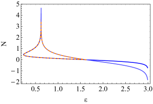
Figure 1: Evolution for $\mathcal{N}=50$ fields using the analytical solution (solid lines) versus the solution obtained with numerical integration (orange dashed lines). The solid lines extrapolate up to kinetic domination showing that is the past attractor.

Finally, we provide some physical insight on the terms $A_{i}v_{i}$ and $A_{i}p_{i}$. Their physical significance becomes more apparent if we examine the single-field case where $A_{i}=1$ and the two terms become simply $v_{1}$ and $p_{1}$. When e.g $0<p_{1}<\sqrt{6}$ then the asymptotic value for $v_{1}$ would be $v_{1}=-p_{1}$. If the initial velocity $v_{1}$ is positive then it first has to decrease to zero and then decrease further until it reaches the value $-p_{1}$. Eq. (28) becomes simply

$$v_{1}(\epsilon)=s\sqrt{2\epsilon}\,,$$ (40)

and when s becomes zero we need to switch to the other branch of the solution. For more fields the distinction between the two case is more complicated because all velocities are mixed through the $A_{i}v_{i}$ terms.

III From kinetic domination to accelerating expansion

III.1 How many e-folds before inflation?

For the product-exponential potential the existence of an analytical solution allows us to calculate the number of e-folds the system spends before it approaches the asymptotic solution. For accelerating solutions specifically, $p_{i}$ should be chosen such that $1/2p_{i}p_{i}<1$. If the system starts at a state with $\epsilon_{0}>1$, then the solution (31) provides the necessary number of e-folds before inflation begins.

For an arbitrary potential, one can ask a similar question; assuming that there exists an “asymptotic” state (in practice the slow-roll solution) and that the system begins with initial conditions close to kinetic domination, then how many e-folds are necessary before inflation starts? The exact duration for the passage from a state with $\epsilon>1$ to a state with $\epsilon<1$ requires the full analytical solution, which seems an impossible task. To make some progress, we can construct an estimate based on the previously derived solution (31). This relies on the observation that for small field displacements any continuous function $p_{i}$ can be approximated by its constant part (the first term in the Taylor series) and this gives a first estimate on the total number of e-folds. However, since the value of $p_{i}$ changes we do not know a priori which value to choose. In the following we will show that in general the minimum and maximum values of $p_{i}$ give the minimum and maximum number of e-folds respectively. To prove this we will first derive some properties of the solutions for product-exponential potentials.

In Fig. 2 we plot the solution for three different exponential potentials ($V_{p}\propto e^{p_{i}\phi_{i}}$ and $V_{\lambda}\propto e^{\lambda_{i}\phi_{i}}$) satisfying $0<p_{i}<\lambda_{i}$ and for positive (upper plot) or negative (lower plot) initial velocities that are close to kinetic domination. In the first case, $v_{(i)}p_{(i)},v_{(i)}\lambda_{(i)}>0$ holds for each $i$ (with no sum implied), while in the second one $v_{(i)}p_{(i)},v_{(i)}\lambda_{(i)}<0$. In the upper plot, $\epsilon$ first decreases until the value $\epsilon_{*}$ and then it increases again until it reaches its asymptotic value. During the decreasing period we observe that steeper gradients lead to faster decrease, whereas this behaviour is reversed once $\epsilon$ starts to increase. This makes sense physically because in the first case the Hubble friction cooperates with the gradient term (until the velocities change sign) and hence $\epsilon$ decreases faster for steeper gradients; similarly, when the velocities increase steeper gradients lead to larger terminal velocities and hence the system needs more time to reach those values. However, in both plots the system reaches its asymptotic state slower for steeper gradients.

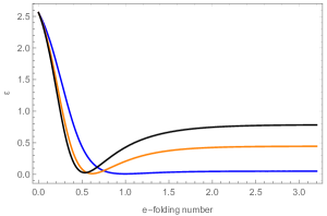
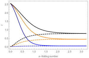
Figure 2: Evolution of 3 product-exponential potentials with $(p_{1},p_{2})$ $=(0.1,0.3)$, $(0.5,0.8)$, $(0.6,1.1)$ (blue, orange and black accordingly). Upper graph: initial velocities are $v_{i,0}=1.6$. Lower graph: initial velocities are negative with $v_{i,0}=-1.6$ (solid lines) or $v_{i,0}=-0.1$ (dashed lines) indicating supercritical or subcritical initial values.

In certain cases we can understand the previous behaviour analytically. For two different product-exponential potentials with $0<|p_{i}|<|\lambda_{i}|$ we obtain $0<|v_{i}p_{i}|<|v_{i}\lambda_{i}|$. When each velocity $v_{i}$ has sign opposite to $p_{i},\lambda_{i}$ then

$$|p_{i}|<|\lambda_{i}|\Rightarrow v_{i}p_{i}>v_{i}\lambda_{i}\,,$$ (41)

and we obtain the following inequality

$$(3-\epsilon)(2\epsilon+p_{i}v_{i})>(3-\epsilon)(2\epsilon+\lambda_{i}v_{i})\,.$$ (42)

Using equation (17) it is transformed into a differential inequality

$${\,\mathrm{d}\epsilon\over\,\mathrm{d}N}<{\,\mathrm{d}\tilde{\epsilon}\over\,\mathrm{d}N}\Rightarrow\epsilon(N)<\tilde{\epsilon}(N)\,,$$ (43)

where we solved the differential equations with equal initial conditions $\epsilon(N_{0})=\tilde{\epsilon}(N_{0})$. In the opposite case where velocities have all the same sign with $p_{i},\lambda_{i}$ then the previous inequality is reversed. In order for this inequality to be satisfied $\epsilon$ should adjust the rate of change according to the magnitude of the gradients. This is exactly what is depicted e.g. in the lower plot of Fig. 2; we observe that for the three sets of exponents $\epsilon(N)$ follows the same inequalities and hence, schematically we have black ¿ orange ¿blue.

A different way to view the previous is that for a given set of $p_{i}$ we can find two different sets of exponents, e.g. $\lambda_{i}$ and $\kappa_{i}$, whose solutions bound the solution for $p_{i}$ at all times. In the derivation of these relations the strict inequality between the different pairs of exponents is crucial; the condition on the norm of the gradient vector $|\kappa|^{2}<|p|^{2}<|\lambda|^{2}$ is not sufficient to provide a bound on $\epsilon$ at all times (see Fig. 2). The inequalities should instead be satisfied for each individual component. Moreover, we required that each velocity should have either the same sign as the corresponding gradient or opposite sign; if this is not satisfied this method may fail to provide definite inequalities for $\epsilon$. This property of the solutions can provide some conclusions about the evolution of more general potentials. For field-dependent $p_{i}(\phi_{j})$, we can estimate the number of e-folds by considering the minimum and maximum values for $p_{i}(\phi_{j})$ in some field interval $[\phi_{j,\rm min},\phi_{j,\rm max}]$. Using these values we calculate $N_{\rm min}$ and $N_{\rm max}$ that correspond to the the solutions for product exponential potentials ($e^{p_{i,\rm min}\phi_{i}}$ and $e^{p_{i,\rm max}\phi_{i}}$ respectively) and then estimate the actual transitional time in the interval $N\in(N_{\rm min},N_{\rm max})$.

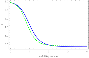
Figure 3: Evolution of 2 product-exponential potentials with $(p_{1},p_{2})=(0.6,0.6)$ and $(\lambda_{1},\lambda_{2})=(0.01,0.9)$ (blue and green dashed accordingly) for negative supercritical velocities with the same $\epsilon_{0}$. Even though $|p|^{2}<|\lambda|^{2}$ the two lines cross.

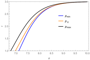
Figure 4: Estimation of $\epsilon$ for a quartic potential using two exponential potentials with $p_{min}=4/\phi_{0}$ and $p_{max}=4/\phi_{*}$ for negative velocities, $\epsilon_{0}=2.99$ and $\phi_{0}=10M_{pl}$.

As an illustrative example we will study quartic inflation $V\sim\phi^{4}/4$. We set the initial conditions to $\phi_{0}=10$ and $\epsilon_{0}=2.99$. The field flows to the origin and in the interval $(0,\phi_{0})$ the gradient $p=4/\phi$ is a monotonically decreasing function; therefore, the minimum value for $p$ would be given by $p(\phi_{0})$, whereas the maximum value corresponds to the value of $\phi$ which gives $\epsilon(\phi_{*})=1$. The latter value is unknown, as we do not know the full solution; in the following we will demonstrate how to estimate it. The value $\phi_{*}$ would be the displacement one would find using the analytical solution (33) if the value $p(\phi_{*})$ was used for the gradient term

$$\phi_{*}=\phi_{0}+\Delta\phi(\epsilon=1,\epsilon_{0},p(\phi_{*}))\,.$$ (44)

Note that the previous is a transcendental equation for $\phi_{*}$. Once this value is known, then $p_{\rm max}=p(\phi_{*})$ can be used in (31) to find the maximum number of e-folds. The precision of this estimate is portrayed in Fig. 4 and we can predict a priori the field displacement between 2.9-3.2 in units of $M_{\rm pl}$, whereas the usual estimation resulting from considering kinetic domination with $p=0$ gives $\Delta\phi=2.35~{}M_{\rm pl}$. This difference, although small, can potentially be important in the light of different conjectures which severely restrict the allowed superplankian field displacement, as well as the minimum value of $p$ Obied:2018sgi ; Agrawal:2018own . Conversely, at a given point $\phi_{0}$ one can constrain $\epsilon_{0}$ by the requirement of 50-60 e-folds of inflation and therefore estimate the “basin of attraction” of the initial conditions that provide sufficient inflation.

III.2 The gradient-flow approximation

For potentials with slowly varying gradients (in some field interval) the two estimated values for $\epsilon$ will be very close. This implies that the system behaves closely to a product exponential with field-dependent exponents, which, nevertheless, satisfy $p_{i}^{\prime}\ll 1$. Moreover, the scaling relations for the velocities $v_{i}\approx-p_{i}$ imply that $\epsilon$ varies slowly

$$\left({1\over 2}p_{i}p_{i}\right)^{\prime}\approx-{V_{,k}V_{,i}V_{,ik}\over V^{2}}+(2\epsilon_{V})^{2}\,,$$ (45)

and the two terms should be small. In the latter equation we recognise the conditions for the validity of the gradient-flow approximation Lyth:2009zz ; Yang:2012bs ; GrootNibbelink:2000vx ; GrootNibbelink:2001qt ; Peterson:2010np ; Peterson:2011ytETAL . Therefore, models that are approximated well by gradient flow lie at the intersection between de Sitter and scaling solutions. The reason why these models asymptote to a state with almost vanishing accelerations can be explained by the fact that they are small deformations of de Sitter-scaling models, which have identically zero accelerations; since they are not exactly product-exponentials, during their evolution they move adiabatically between asymptotic solutions of exponentials. In this way, one can deduce the global convergence towards the slow-roll solution which can not be done using linearised analysis. As a final remark, the scaling relations fix the fields’ velocities, through $v_{i}\approx-p_{i}$, but not their position. Therefore, under this type of approximation observables inherit an explicit dependence on (a subset of) initial conditions.

IV Generalizations

In addition to the scalar fields we will consider a non-interacting fluid with an equation of state $P=w\rho$. The Klein-Gordon equations remain unchanged, while Eqs. (4) and (5) are modified

$$3H^{2} =\frac{1}{2}\dot{\phi}_{i}\dot{\phi}_{i}+V+\rho\,.$$ (46)

$$\dot{H} =-\frac{1}{2}\dot{\phi}_{i}\dot{\phi}_{i}-\frac{1}{2}(1+w)\rho\,,$$ (47)

and we obtain an additional equation, the conservation equation for the fluid,

$$\dot{\rho}+3H(1+w)\rho=0\,.$$ (48)

The slow-roll parameter is now given by

$$\epsilon=\frac{1}{2}v_{i}v_{i}+{1\over 2}(w+1){\rho\over H^{2}}\,.$$ (49)

Introducing a new variable $z\equiv\rho/H^{2}$ and using

$${V\over H^{2}}=3-\epsilon+{1\over 2}(w-1)z\,,$$ (50)

the system of evolution equations can be written as

$$v_{i}^{\prime}+(3-\epsilon)(v_{i}+p_{i})+{1\over 2}(w-1)zp_{i}=0\,,$$ (51)

$$z^{\prime}+\left(3+3w-2\epsilon\right)z=0\,.$$ (52)

In this form one can immediately read off asymptotic solutions, generalizing the solutions for one field (see e.g. Copeland:1997et )

1. scalar kinetic domination: $z=0$, $\epsilon=3$. There exists an infinite number of field realizations describing kinetic domination, namely all points on the hypersphere satisfying $v_{i}v_{i}=6$.

2. scalar potential domination: $z=0$, $v_{i}=-p_{i}$ with $\epsilon=1/2p_{i}p_{i}$.

3. fluid domination: $v_{i}=0$, $z=3$ with $\epsilon=3/2(1+w)$.

4. scaling solution: fields and fluid are non-zero with $\epsilon=3/2(1+w)$ (the expressions for $v_{i}$ and $z$ are more complicated but can be found by solving quadratic equations).

In the case of a fluid with $w=1$  equations simplify to

$$v_{i}^{\prime}+(3-\epsilon)(v_{i}+p_{i})=0\,,$$ (53)

$$z^{\prime}+\left(3-\epsilon\right)2z=0\,,$$ (54)

and, hence, one obtains another integral of motion which can be used to express the fluid in terms of a reference field

$$z={z_{0}\over\left(v_{1,0}+p\right)^{2}}\left(v_{1}+p\right)^{2}\equiv{B\over 2}\left(v_{1}+p\right)^{2}\,.$$ (55)

Plugging back into the slow-roll parameter (49) we obtain

$$2\epsilon=\sum_{i=1}^{\mathcal{N}}(A_{i}(v_{1}+p_{1})-p_{i})^{2}+B(v_{1}+p_{1})^{2}\,,$$ (56)

which has the same form as Eq. (24) after the substitution $A^{2}\rightarrow\tilde{A}^{2}=A^{2}+B$. Moreover, for $w=1$ Eq. (17) remains unchanged and the general solution in terms of $\epsilon$ has exactly the same form (Eqs. (31) and (33)) modulo the substitution $A^{2}\rightarrow\tilde{A}^{2}$.

V Summary and discussion

Scalar fields in cosmology have been extensively studied over the last decades mainly due to their applications in both the early and the late universe. To date, only a limited number of exact solutions exists in the literature. In this paper we derived the general solution for an interacting product-exponential potential, that has not been considered in earlier works, in terms of the slow-roll parameter $\epsilon$. In the latter form it better highlights properties of its critical points.

We argued how the solution becomes relevant in the derivation of estimates for the transitional time to inflation for models that follow the potential gradient flow. For the non-linear evolution towards the slow-roll solution, i.e. starting with arbitrarily large deformations, one needs the full solution. Since there is no general prescription on how to solve the Klein-Gordon equation, one can alternatively derive estimates for the time of this transition using the solution of exponential potentials. This method generalizes the existing estimates, as it does not assume kinetic domination or negligible potential gradients $K\gg V,V_{,\phi}$ (that was considered in previous works, e.g. Goldwirth:1991rj ). We showed that the actual transitional time will lie between two bounds that depend on magnitude of the potential gradient $(\ln V)_{,\phi}$. Besides providing more accurate results the method can be applied in multi-field models where linearized stability becomes obscure due to the coupling of fields’ perturbations.

It is worth noticing that the general solutions presented in this work can also describe multi-field domain walls. The correspondence between cosmological and domain wall solutions can be found e.g. in the Refs. Skenderis:2006rr ; Skenderis:2007sm ; McFadden:2009fg ; Garriga:2014fda . The beta function is the analogue of the slow-roll parameter $\epsilon$ and hence the RG flow of multi-field domain walls with product exponential potentials can be found using the solutions (31) and (33) and the dictionary between cosmology and domain walls.

Finally, we considered the case of an extra non-interacting fluid. When the fluid obeys an equation of state $w=1$ (stiff matter) another integral of motion exists which makes the problem again fully integrable with almost the same solution as before (more precisely with a minor subsitution). It would be interesting to investigate how this solution can be generalized for problems with non-trivial field manifolds.

References

- (1) Y. Akrami et al. [Planck Collaboration], “Planck 2018 results. X. Constraints on inflation,” arXiv:1807.06211 [astro-ph.CO].
- (2) A. A. Starobinsky, “A New Type of Isotropic Cosmological Models Without Singularity,” Phys. Lett. 91B, 99 (1980) [Adv. Ser. Astrophys. Cosmol. 3, 130 (1987)].
- (3) K. Sato, “Cosmological Baryon Number Domain Structure and the First Order Phase Transition of a Vacuum,” Phys. Lett. 99B, 66 (1981) [Adv. Ser. Astrophys. Cosmol. 3, 134 (1987)].
- (4) K. Sato, “First Order Phase Transition of a Vacuum and Expansion of the Universe,” Mon. Not. Roy. Astron. Soc. 195, 467 (1981).
- (5) D. Kazanas, “Dynamics of the Universe and Spontaneous Symmetry Breaking,” Astrophys. J. 241, L59 (1980).
- (6) A. H. Guth, “The Inflationary Universe: A Possible Solution to the Horizon and Flatness Problems,” Phys. Rev. D 23, 347 (1981) [Adv. Ser. Astrophys. Cosmol. 3, 139 (1987)].
- (7) A. D. Linde, “A New Inflationary Universe Scenario: A Possible Solution of the Horizon, Flatness, Homogeneity, Isotropy and Primordial Monopole Problems,” Phys. Lett. 108B, 389 (1982) [Adv. Ser. Astrophys. Cosmol. 3, 149 (1987)].
- (8) A. Albrecht and P. J. Steinhardt, “Cosmology for Grand Unified Theories with Radiatively Induced Symmetry Breaking,” Phys. Rev. Lett. 48, 1220 (1982) [Adv. Ser. Astrophys. Cosmol. 3, 158 (1987)].
- (9) L. C. Price, J. Frazer, J. Xu, H. V. Peiris and R. Easther, “MultiModeCode: An efficient numerical solver for multifield inflation,” JCAP 1503, 005 (2015) [arXiv:1410.0685 [astro-ph.CO]].
- (10) M. Dias, J. Frazer and D. Seery, “Computing observables in curved multifield models of inflation—A guide (with code) to the transport method,” JCAP 1512 (2015) 030 [arXiv:1502.03125 [astro-ph.CO]].
- (11) M. Dias, J. Frazer, D. J. Mulryne and D. Seery, “Numerical evaluation of the bispectrum in multiple field inflation—the transport approach with code,” JCAP 1612, 033 (2016) [arXiv:1609.00379 [astro-ph.CO]].
- (12) J. W. Ronayne and D. J. Mulryne, “Numerically evaluating the bispectrum in curved field-space— with PyTransport 2.0,” JCAP 1801, 023 (2018) [arXiv:1708.07130 [astro-ph.CO]].
- (13) D. J. Mulryne and J. W. Ronayne, “PyTransport: A Python package for the calculation of inflationary correlation functions,” J. Open Source Softw. 3, no. 23, 494 (2018) [arXiv:1609.00381 [astro-ph.CO]].
- (14) D. S. Salopek and J. R. Bond, “Nonlinear evolution of long wavelength metric fluctuations in inflationary models,” Phys. Rev. D 42, 3936 (1990).
- (15) L. P. Chimento, “General solution to two-scalar field cosmologies with exponential potentials,” Class. Quant. Grav. 15, 965 (1998).
- (16) J. G. Russo, “Exact solution of scalar tensor cosmology with exponential potentials and transient acceleration,” Phys. Lett. B 600, 185 (2004) [hep-th/0403010].
- (17) E. Elizalde, S. Nojiri and S. D. Odintsov, “Late-time cosmology in (phantom) scalar-tensor theory: Dark energy and the cosmic speed-up,” Phys. Rev. D 70, 043539 (2004) [hep-th/0405034].
- (18) R. de Ritis, G. Marmo, G. Platania, C. Rubano, P. Scudellaro and C. Stornaiolo, “New approach to find exact solutions for cosmological models with a scalar field,” Phys. Rev. D 42, 1091 (1990).
- (19) A. A. Andrianov, F. Cannata and A. Y. Kamenshchik, “General solution of scalar field cosmology with a (piecewise) exponential potential,” JCAP 1110, 004 (2011) [arXiv:1105.4515 [gr-qc]].
- (20) D. Bertacca, S. Matarrese and M. Pietroni, “Unified Dark Matter in Scalar Field Cosmologies,” Mod. Phys. Lett. A 22, 2893 (2007) [astro-ph/0703259 [ASTRO-PH]].
- (21) E. Piedipalumbo, P. Scudellaro, G. Esposito and C. Rubano, “On quintessential cosmological models and exponential potentials,” Gen. Rel. Grav. 44, 2611 (2012) [arXiv:1112.0502 [astro-ph.CO]].
- (22) S. Basilakos, M. Tsamparlis and A. Paliathanasis, “Using the Noether symmetry approach to probe the nature of dark energy,” Phys. Rev. D 83, 103512 (2011) [arXiv:1104.2980 [astro-ph.CO]].
- (23) A. Paliathanasis, M. Tsamparlis and S. Basilakos, “Dynamical symmetries and observational constraints in scalar field cosmology,” Phys. Rev. D 90, no. 10, 103524 (2014) [arXiv:1410.4930 [gr-qc]].
- (24) M. Tsamparlis and A. Paliathanasis, “Lie and Noether symmetries of geodesic equations and collineations,” Gen. Rel. Grav. 42, 2957 (2010) [arXiv:1101.5769 [gr-qc]].
- (25) M. Tsamparlis and A. Paliathanasis, “Two dimensional dynamical systems which admit Lie and Noether symmetries,” J. Phys. A 44, 175202 (2011) [arXiv:1101.5771 [math-ph]].
- (26) Y. Zhang, Y. g. Gong and Z. H. Zhu, “Noether Symmetry Approach in multiple scalar fields Scenario,” Phys. Lett. B 688, 13 (2010) [arXiv:0912.0067 [hep-ph]].
- (27) A. Paliathanasis and M. Tsamparlis, “Two scalar field cosmology: Conservation laws and exact solutions,” Phys. Rev. D 90, no. 4, 043529 (2014) [arXiv:1408.1798 [gr-qc]].
- (28) L. Anguelova, E. M. Babalic and C. I. Lazaroiu, “Two-field Cosmological -attractors with Noether Symmetry,” arXiv:1809.10563 [hep-th].
- (29) A. Paliathanasis, G. Leon and S. Pan, “Exact Solutions in Chiral Cosmology,” Gen. Rel. Grav. 51 (2019) no.9, 106 [arXiv:1811.10038 [gr-qc]].
- (30) M. Tsamparlis, A. Paliathanasis and L. Karpathopoulos, “Autonomous three-dimensional Newtonian systems which admit Lie and Noether point symmetries,” J. Phys. A 45, no. 27, 275201 (2012) [arXiv:1111.0810 [physics.class-ph]].
- (31) F. Lucchin and S. Matarrese, “Power Law Inflation,” Phys. Rev. D 32, 1316 (1985).
- (32) J. J. Halliwell, “Scalar Fields in Cosmology with an Exponential Potential,” Phys. Lett. B 185, 341 (1987).
- (33) P. J. Steinhardt, L. M. Wang and I. Zlatev, “Cosmological tracking solutions,” Phys. Rev. D 59, 123504 (1999) [astro-ph/9812313].
- (34) A. Nunes and J. P. Mimoso, “On the potentials yielding cosmological scaling solutions,” Phys. Lett. B 488, 423 (2000) [gr-qc/0008003].
- (35) A. R. Liddle, A. Mazumdar and F. E. Schunck, “Assisted inflation,” Phys. Rev. D 58, 061301 (1998) [astro-ph/9804177].
- (36) K. A. Malik and D. Wands, “Dynamics of assisted inflation,” Phys. Rev. D 59, 123501 (1999) [astro-ph/9812204].
- (37) E. J. Copeland, A. Mazumdar and N. J. Nunes, “Generalized assisted inflation,” Phys. Rev. D 60, 083506 (1999) [astro-ph/9904309].
- (38) S. V. Chervon, V. M. Zhuravlev and V. K. Shchigolev, “New exact solutions in standard inflationary models,” Phys. Lett. B 398, 269 (1997) [gr-qc/9706031].
- (39) R. Easther, “Exact superstring motivated cosmological models,” Class. Quant. Grav. 10, 2203 (1993) [gr-qc/9308010].
- (40) S. V. Chervon, I. V. Fomin and A. Beesham, “The method of generating functions in exact scalar field inflationary cosmology,” Eur. Phys. J. C 78, no. 4, 301 (2018) [arXiv:1704.08712 [gr-qc]].
- (41) J. Martin, C. Ringeval and V. Vennin, “Encyclopædia Inflationaris,” Phys. Dark Univ. 5-6, 75 (2014) [arXiv:1303.3787 [astro-ph.CO]].
- (42) I. Y. Aref’eva, N. V. Bulatov and S. Y. Vernov, “Stable Exact Solutions in Cosmological Models with Two Scalar Fields,” Theor. Math. Phys. 163, 788 (2010) [arXiv:0911.5105 [hep-th]].
- (43) D. Bazeia, L. Losano and J. R. L. Santos, “Kinklike structures in scalar field theories: from one-field to two-field models,” Phys. Lett. A 377, 1615 (2013) [arXiv:1304.6904 [hep-th]].
- (44) P. H. R. S. Moraes and J. R. L. Santos, “Two scalar field cosmology from coupled one-field models,” Phys. Rev. D 89, no. 8, 083516 (2014) [arXiv:1403.5009 [gr-qc]].
- (45) N. Dimakis, A. Paliathanasis, P. A. Terzis and T. Christodoulakis, “Cosmological Solutions in Multiscalar Field Theory,” Eur. Phys. J. C 79 (2019) no.7, 618 [arXiv:1904.09713 [gr-qc]].
- (46) D. S. Goldwirth and T. Piran, “Initial conditions for inflation,” Phys. Rept. 214, 223 (1992).
- (47) G. Obied, H. Ooguri, L. Spodyneiko and C. Vafa, “De Sitter Space and the Swampland,” [arXiv:1806.08362 [hep-th]].
- (48) P. Agrawal, G. Obied, P. J. Steinhardt and C. Vafa, “On the Cosmological Implications of the String Swampland,” Phys. Lett. B 784 (2018), 271-276 [arXiv:1806.09718 [hep-th]].
- (49) P. Christodoulidis, D. Roest and E. I. Sfakianakis, “Scaling attractors in multi-field inflation,” JCAP 12, 059 (2019) [arXiv:1903.06116 [hep-th]].
- (50) E. J. Copeland, A. R. Liddle and D. Wands, “Exponential potentials and cosmological scaling solutions,” Phys. Rev. D 57 (1998), 4686-4690 [arXiv:gr-qc/9711068 [gr-qc]].
- (51) V. Faraoni, “The correspondence between a scalar field and an effective perfect fluid,” Phys. Rev. D 85 (2012), 024040 [arXiv:1201.1448 [gr-qc]].
- (52) D. H. Lyth and A. R. Liddle, “The primordial density perturbation: Cosmology, inflation and the origin of structure,” Cambridge, UK: Cambridge Univ. Pr. (2009) 497 p
- (53) I. S. Yang, “The Strong Multifield Slowroll Condition and Spiral Inflation,” Phys. Rev. D 85, 123532 (2012) [arXiv:1202.3388 [hep-th]].
- (54) S. Groot Nibbelink and B. J. W. van Tent, “Density perturbations arising from multiple field slow roll inflation,” hep-ph/0011325 ;
- (55) S. Groot Nibbelink and B. J. W. van Tent, “Scalar perturbations during multiple field slow-roll inflation,” Class. Quant. Grav. 19, 613 (2002) [hep-ph/0107272].
- (56) C. M. Peterson and M. Tegmark, “Testing Two-Field Inflation,” Phys. Rev. D 83, 023522 (2011) [arXiv:1005.4056 [astro-ph.CO]] ;
- (57) C. M. Peterson and M. Tegmark, “Testing multifield inflation: A geometric approach,” Phys. Rev. D 87, no. 10, 103507 (2013) [arXiv:1111.0927 [astro-ph.CO]] ;
- (58) K. Skenderis and P. K. Townsend, “Hamilton-Jacobi method for curved domain walls and cosmologies,” Phys. Rev. D 74 (2006), 125008 [arXiv:hep-th/0609056 [hep-th]].
- (59) P. McFadden and K. Skenderis, “Holography for Cosmology,” Phys. Rev. D 81 (2010), 021301 [arXiv:0907.5542 [hep-th]].
- (60) J. Garriga, K. Skenderis and Y. Urakawa, “Multi-field inflation from holography,” JCAP 01 (2015), 028 [arXiv:1410.3290 [hep-th]].
- (61) K. Skenderis, P. K. Townsend and A. Van Proeyen, “Domain-wall/cosmology correspondence in adS/dS supergravity,” JHEP 08 (2007), 036 [arXiv:0704.3918 [hep-th]].