Adversarial Resilience Learning — Towards Systemic Vulnerability Analysis for Large and Complex Systems

Abstract.

This paper introduces Adversarial Resilience Learning (ARL), a concept to model, train, and analyze artificial neural networks as representations of competitive agents in highly complex systems. In our examples, the agents normally take the roles of attackers or defenders that aim at worsening or improving—or keeping, respectively—defined performance indicators of the system. Our concept provides adaptive, repeatable, actor-based testing with a chance of detecting previously unknown attack vectors. We provide the constitutive nomenclature of ARL and, based on it, the description of experimental setups and results of a preliminary implementation of ARL in simulated power systems.

1. Introduction

color=green!40]EVe: Better start: this is very abrupt. Add some intro text.

Current newspapers are full of horrific tales of “cyber-attackers” threatening our energy systems. And, if not for the notorious “evil state”-actor, it is the ongoing digitization necessary to enable increasing renewable and volatile energy generation that threatens our energy supply and thus the stability of our society. And while the main approach seems to be to patch-up the detected vulnerabilities of protocols, software and controller devices, our approach is to research and develop the means to systematically design and test systems that are structurally resilient against failures and attackers alike.

Security in cyber-systems mostly should be concerned with establishing asymetric control in favour of the operator of a system. In order to achieve this on a structural level at design time, reproducible benchmark tests are required. This is notoriously difficult for intelligent adversaries whose primary ability are adaption and creativity. Thus, testing methods nowadays are either reproducible and insufficiently modelling attacker — or they involve unreproducible human elements. Reinforcement learning may be useful to provide at least some adaptability of reproducible attacker models.

This work takes its motivation and first practical implementation from the power system domain, but the work can directly be applied to all highly complex, critical systems. Systems that may benefit from Adversarial Resilience Learning (ARL) are too complex to be sufficiently described using analytic methods, i. e., because the number of potential states is to large and the behaviour is too complex with too many non-trivial interdependencies.

This work introduces ARL, which provides a method to analyse complex interdependent systems with respect to adversarial actors. The foremost motivation is to provide a method for deterministic analysis method for complex and large systems including some degree of adaptivity of the simulated attackers.

The main contribution of this paper is the introduction of a novel structure for training and application of Artificial Neural Networks (ANNs) that generalizes the approach of adversarial learning. By setting up ANN-based agents in a competitive situation, the learning-complexity is comprised not only of a highly complex system, but also of competing ANNs whose changing state, manifested by modified behaviour of the system under consideration, has to be included in the trained model. We assume that this provides a very interesting new problem class for Reinforcement Learning (RL), as it introduces a cyclic learning competition.

The paper is structured as follows. First, a brief introduction into related techniques in machine learning and related work for complex system analysis is given. The paper then defines the concept of Adversarial Resilience Learning in Section 3, and introduces its application to adversary testing in power system control in Section 4. The paper is completed by a presentation of lessons’ learned and results from an early proof-of-concept demonstrator in Section 4.2. Itconcludes with a discussion and an outlook in Section 5

2. Related Work

This work aims at exploring the feasibility of improving resilience of complex systems using machine learning to train adaptive agents. The term resilience is lacking a coherent and precise definition across fields. Generally it denotes the ability of a system to withstand unforseen, rare and potentially catastrophic events, recover from the damage and adapt by improving itself in reaction to these events. Ideally, resilience is increasing monotonously throughout system improvement. A useful simplification is observation of the changing behaviour of system performance as an artefact resulting from resilience processes. Different formalisation of resilience processes exist, but most distinguish subprocesses for planning, absorbtion of damage, recovery (or self-healing) and improvement (or adaption). (Arghandeh et al., 2016)

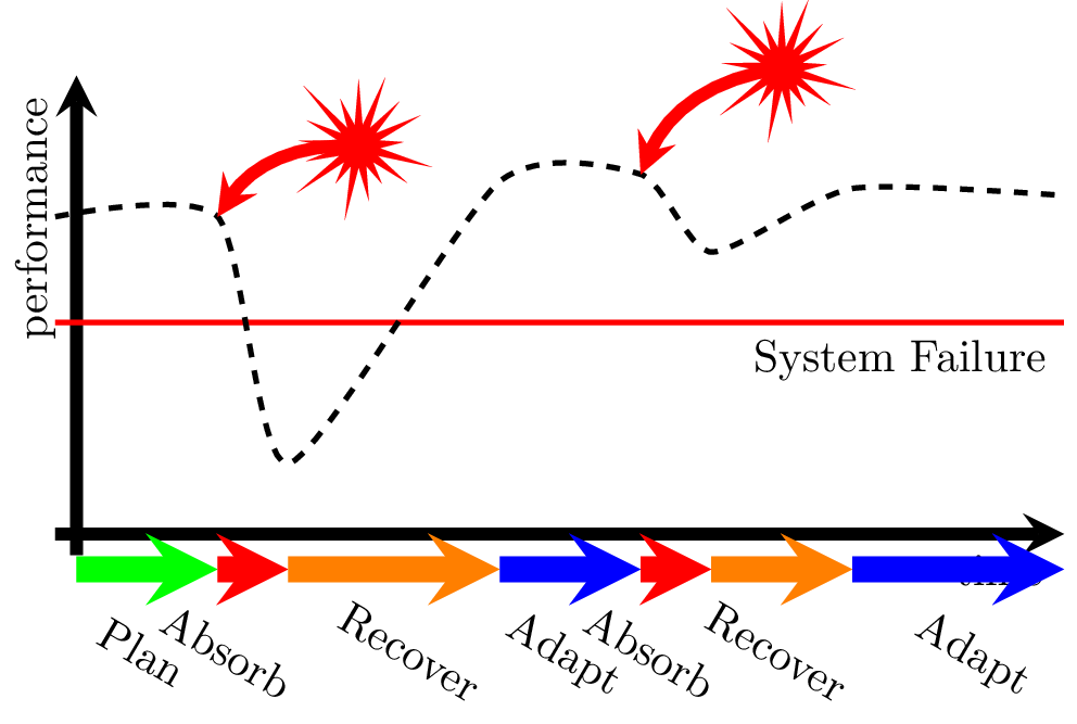
See Figure 1 for an expression of a hypothetical system’s performance suffering twice from damaging events. Resilience is modelled as a sequential process: Plan, Absorb, Recover and Adapt. (Linkov and Kott, 2019) As consequence of the first event the performance of the system is pushed below a failure threshold, i. e., the system fails to provide its service. Improvement of the system is then achieved after recovery as the system is able to keep the performance above the failure threshold during the second event.

Figure 1. Resilience Process for system performance

2.1. Analysis and Stochastic Modelling

The main distinction of our approach as compared to game theoretic modelling and stochastic analysis is the use of co-simulation and heuristic approaches instead of formal abstraction of complete systems. The underlying assumption is, that a system-of-systems is too complex, and malicious adversaries are too unpredictable to be sufficiently analysed.

But similarly to Attacker-Defender Models, e. g., described in (Brown et al., 2006) that at analysing an equilibrium between attackers and defenders in dynamic systems, our work aims at heuristically approach an estimate of the asymmetry of attacker and defender in these systems. The approach of ARL structurally similar to the concept of Stackleberg Competition and related applications of stochastic analysis, e. g., pursuit-evasion in differential games (Isaacs, 1965). These approaches seem to only be applicable to scenarios that can be restricted to few degrees of freedom. More realistic behaviours of opportunistically acting threat agents within complex system-of-systems leads to an explosion of states in analytic approaches.

Recent surveys seem to support this view. Referenced approaches on power systems in (Do et al., 2017) provide no details on the used game-theoretic model and use ambiguous terminology of the researched threat scenarios. Approaches in Machine Learning (ML) to tackle complex problems, on the other hand, have, not only recently, been very successful in providing novel, practical solutions.

2.2. Machine Learning

ANNs are universal function approximators, meaning that they can be used as a statistical model of any Borel-measurable function $\mathbb{R}^{n}\mapsto\mathbb{R}^{m}$ with desired non-zero error (Cybenko, 1989; Hornik et al., 1989; Goodfellow et al., 2016). Already the standard Recurrent Neural Network (RNN) (e. g., Elman (1990)) has the capacity to approximate any non-linear dynamic system (Seidl and Lorenz, 1991), and Siegelmann and Sonntag have shown that RNNs are turing-complete (Siegelmann and Sontag, 1995).

In practice, a typical problem for which RNNs, especially structures containing Long-Short Term Memory (LSTM) cells (Hochreiter and Schmidhuber, 1997) or Gated Recurrent Units (GRUs) (Cho et al., 2014; Chung et al., 2014) are used, is time series prediction. Even greater memory capacity is achieved by neural turing machines, introduced by Graves et. al. (Graves et al., 2014), which also counter the learning problem that is inherent to the turing-completeness of RNNs: in theory, a RNNs have the capacity to simulate arbitrary procedures, given the proper set of parameters; in practice, this training task has proven to be complicated. Neural Turing Machines counter the complexity with a vastly increased addressable memory space and have shown to be able to simulate simple, but complete algorithms like sorting [ibd.].

Predicting a time series with an RNN constitutes the instantiation of a (non-linear) dynamic system (Tong, 1990; Basharat and Shah, 2009; Yu et al., 2007), i. e., the prediction is the result of the system’s behavior, which is, in turn, modeled and approximated by the RNN. Cessac has examined ANNs from the perspective of dynamical systems theory, characterizing also the collective dynamics of neural network models (Cessac, 2010).

Different ways exist to train ANNs and RNNs. When using supervised training methods, the training set consists of both, vectors of input and known output the ANN is expected to exhibit. Two different classes of training algorithms are popular for this type of training, with gradient-decent-based algorithms of the Backpropagation-of-Error family leading by far (Rumelhart et al., 1986; Kingma and Ba, 2014; Dozat, 2016; Ruder, 2016; Cuéllar et al., 2007), followed by evolutionary algorithms such as CMA-ES (Hansen, 2006; Ros and Hansen, 2008; Hansen et al., 2003) or REvol (Ruppert et al., 2014; Veith, 2017). However, all optimization methods adapt the ANN to minimize a cost function and not directly to create a model of a problem; this happens only indirectly. As a result, ANNs can still be “foiled,” i. e., made to output widely wrong results in the face of only minor modifications to the input. This effect and how to counter it is the subject of adversarial learning research.

With unsupervised learning, the ANN tries to detect patterns in the input data that diverge from the background noise. Unsupervised learning does not use the notion of expected output (Ghahramani, 2004). A modern application of unsupervised learning has emerged in the concept of Generative Adversarial Networks (GANs). Here, one network, called the generator network, creates solution candidates—i. e.,maps a vector of latent variables to the solution space—, which are then evaluated by a second network, the discriminator (Goodfellow et al., 2014). Ideally, the result of the training process are results virtually indistinguishable from the actual solution space, which is the reason GANs are sometimes called “Turing learning.” The research focus of ARL is not the generation of realistic solution candidates; this is only a potential extension of the attackers and defenders themselves. ARL, however, describes the general concept of two agents influencing a common model but with different sensors (inputs) and actuators (output) and without knowing of each others presence or actions.

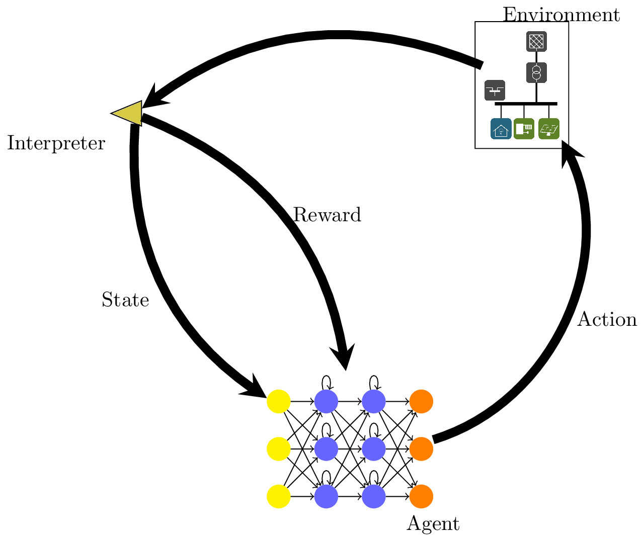
RL (III, 1994) describes a third class of learning algorithms. It extends the process of adapting the weight matrix of any ANN by including the notion of an environment into the training process. In RL, an agent interacts with its environment that provides it with feedback, which can be positive or negative. The agent’s goal is to maximize its reward. The agent internally approximates a reward function in order to achieve a high reward through actions for every state of its environment. Initially, RL was not tied to ANNs (Minsky, 1954). However, as the environment becomes more complex, so does the agent’s reward function; ANNs are very well suited for function approximation or, if the reward is based on a complex state of a world, i. e., a dynamic system, RNNs are suitable.

For ARL, we assume a common model that is used by two distinct agents: while one probes the model for weaknesses in order to find attack vectors, the other monitors the system and, unbeknowing of the presence of the attacker or its actions, works at keeping the system in its nominal state. Through this structure, the notion of ARL assumes that the model—i. e., each agent’s environment—is not completely known to the respective agent. Therefore, the usage of RL readily suggests itself.

The abstract notion of a model can see multiple instantiations; one such instantiation of ARL would be using a power grid as the model considered by both agents. Ernst et al. employ RL for stability control in power grids (Ernst et al., 2004). In their paper, they design a dynamic brake controller to damp large oscillations; however, since the reward function is easily well-defined, there is no need for using an ANN for function approximation.

Figure 2 shows the general schema of RL, adapted from literature for the power grid as the environment.

Figure 2. Reinforcement Learning

The concept we propose in this paper is related to Adversarial Learning (AL) insofar, as both concepts use two distinct ANNs with conflicting objectives (Goodfellow et al., 2015).

AL is the field of exploiting vulnerabilities in learning algorithms in order to affect the behaviour of the resulting (learned) system. The prevalent technique is specially crafting inputs that lead to unintended patterns being recognised. A secondary objective is to use inputs that are not recognised as disturbing patterns by humans. AL thus are a concept to implement a Stackelberg Competition in neural networks.

A very recent example is given by Evtimov et al. (Evtimov et al., 2017), where the authors showed how they were able to confuse known deep learning image recognition algorithms by attaching markings to physical objects.

AL neural network setups (for non-physical interventions) are characterised by two output layers in sequence. The first output layer functions as the adversary, generating outputs from a given input layer, i. e., the “real world inputs” The second output layer represents the function of the original classifier that has to learn to correctly classify the original inputs despite the adversary’s efforts to scramble the input.

3. Adversarial Resilience Learning

ARL is distinguished from AL by the recurrent structure in which adversary and defender are interacting. While GAN directly connect a generating adversary with a detecting defender, ARL adversary and defender interact only through the system they are using for input and output. In this interaction adversaries are identified as agents inserting disturbances into the system, while defenders provide resilience control.

Definition 3.1 (Adversarial Resilience Learning (informal)).

ARL is an experimental structure comprised of two disjoint groups of agents and a system or simulated system. The agents are distinguished as attacker and defender by adhering to conflicting optimisation objectives. Both groups of agents receive their input from a, potentially overlapping, set of measurements from the system. They influence the system through two disjunct sets of outputs connected to controls in the simulated system.

3.1. Fundamental Notation and Model

The basic abstract scenario using ARL consists of two competing agents and a system model. Each of the three elements resembles a state transition. In order to establish a sound formal base, a definition of notation and processes of ARL is provided here. A summary of notations used is given in section 3.1.

ARL consists of a set of agents, where each agent has a model, denoted by $\mathcal{A}$, and a model of a system, $\mathcal{M}$. The agent model $\mathcal{A}$ serves as a “blue-print” for the actual behavior of a running system; similarly, $\mathcal{M}$ denotes a static model of a world. An index identifies a particular agent model, e. g., $\mathcal{A}_{A}$ denotes the category of attacker models, $\mathcal{A}_{\Omega}$ serves to denote the category of defender models. At run-time, the models are instantiated. We denote instances of a model with lower-case letters $a$, where the index denotes a particular state of the model, such as $a_{t}$ with $t$ commonly referring a point in simulation time. In the same vein, $m$ denotes an instance of a world model.

Each agent tries to maximize its rewards by approximating the agent-specific performance function,

(1) $$p_{a}(m_{t})\leavevmode\nobreak\ .$$

For an agent, the performance function $p_{a}(\cdot)$ is equal to its reward function in RL terminology. However, the notion of the performance function lets us decouple agent behavior from the desired/intended or undesired performance of the world, denoted by

(2) $$p(m_{t})\leavevmode\nobreak\ ,$$

as the difference between the world’s current performance to its nominal performance, $p^{*}$.

Agents are categorized through their performance function, an agent model is identified as attacker model $\mathcal{A}_{A}$ if his reward function $p_{a}$ behaves inverse to the systems performance. The opposite is true for agents from $\mathcal{A}_{\Omega}$. That is, we can define:

Definition 3.2 (Attacker and Defender Classes).

For all times $t$ and model instances $m\in\mathcal{M}$, the following provides a classification rule for attackers and defenders:

(3) $$\begin{array}[]{rcl}a\in\mathcal{A}_{A}&\Rightarrow p_{a}(m_{t})&\nsim p(m_{t}),\\ a\in\mathcal{A}_{\Omega}&\Rightarrow p_{a}(m_{t})&\sim p(m_{t})\leavevmode\nobreak\ .\end{array}$$

The performance of an agent is tightly coupled to an agent’s view of its environment, i. e., the world. Each $p_{a}(\cdot)$ can only be defined in terms of the agent’s sensory inputscolor=green!40]EVe: it is possible to have performance untainted by sensor dilution $\psi$, i. e., the part the world it can observe. The portion of the state of a system instance an agent $a$ can observe is denoted by

(4) $$x_{a,t}=\psi_{a}(m_{t})\leavevmode\nobreak\ .$$

Given the sensory inputs of an agent $a$ at $t$ are given as $x_{a,t}$, the agent can act by approximating its reward function $p_{a}(\cdot)$. This approximation is the agent’s activation of its internal dynamic system approximator $\mathrm{act}(\cdot)$; implemented through, e. g., an RNN, such that

(5) $$\mathrm{act}_{a}:(a_{t},x_{a,t})\mapsto(a_{t+1},y_{a,t+1})\leavevmode\nobreak\ ,$$

where we assume that an agent is always able to observe its environment through $\psi_{a}(m_{t})$, i. e., $|x_{a,t}|>0$, whereas it can choose not to act, i. e., $|y_{a,t+1}|\geq 0$.

An agent then acts on the system model through its actuators’ actions, $y_{a,t}$, which are defined in its respective agent model, where each agent has a specified set of actions of an actuator available at any given time. Each agent defines an action policy for controlling its actuators. In the simple case, the actions of an actuator are mapped from labels $[y_{1},y_{2},\dotsc,y_{m}]^{\top}$ of, e. g., an internal RNN: Each evaluation step of the performance function maps the sensor inputs $x_{a,t}$ onto likelihood values $y_{a,t}$ for all labels of all actuators. The common interpretation is that from each group of labels, the action mapped from the highest-valued label is chosen as the one exerted onto the system by the agent. However generally, an action policy takes on a form that is suitable for the whole action search space, such as a policy network steering a monte carlo tree search as has been shown in (Silver et al., [n. d.]). Thus, an agent is acting through the evaluation and application of its system approximator. This happens for each agent $1,2,\dotsc,n$. In brief, the systems behavior is heavily influenced by the set of all actuators that can be controlled by the respective agents. Thus, an agent does not simple perceive a model (or a part thereof), but the state of the model as the result of all agents acting upon it. Thus, an agent does not simply create an internal representation of a dynamic system, but of a dynamical system-of-systems.

Finally, the simulator evaluates the actions of all agents applied to the world model at $t$, $m_{t}$. This is represented by the evaluation function,

(6) $$\mathrm{eval}:(\bm{y}_{t},m_{t})\mapsto m_{t+1}\leavevmode\nobreak\ ,$$

where the aggregated inputs and outputs over all agents are represented as vectors

(7) $$\bm{x}_{t}=\begin{bmatrix}x_{a_{1},t}\\ \vdots\\ x_{a_{n},t}\\ \end{bmatrix},\quad\bm{y}_{t}=\begin{bmatrix}y_{a_{1},t}\\ \vdots\\ y_{a_{n},t}\\ \end{bmatrix}\leavevmode\nobreak\ .$$

If the activation vectors of the participating agents consider a disjoint set of controllers, i. e., the actions application is commutative, the transition of the world state from $m_{t}$ to $m_{t+1}$ is the result of an aggregation of all agents’ actions $\bm{y}_{t}$. Non-commutative application of actions is out of scope of this work.

o lX   Symbol	Description
$m$ of $\mathcal{M}$	An instance of a system model
$a$ of $\mathcal{A}$	An instance of an agent model
$\mathcal{A}_{A},\mathcal{A}_{\Omega}$	Attacker model, defender model ( Definition 3.2)
$p(\cdot)\in\mathbb{R}_{+}$	Performance function
$p^{*},p^{f}$	Reference performance of normal operation, of failure threshold
$p(m_{t})$	Overall performance of a system instance $m$ at time $t$ (eq. 2)
$p_{a}(m_{t})$	Performance with respect to the objectives of agent instance $a$ at $t$ given the system instance $m$ (eq. 1)
$\psi_{a}$	Observation function mapping a system model $m_{t}$ onto the inputs available to agent $a$, eq. 4
$x_{a,t}$	Inputs to agent $a$ at time $t$, eq. 4
$y_{a,t}$	Actions $y$ of $a$ at $t$, given observable state $x_{a,t}$ (eq. 5)
$\bm{a}_{t}$, $\bm{x}_{t}$, $\bm{y}_{t}$	Vectors of all agents’ states, observable agent inputs, and agent actions corresponding $a$ (eq. 7)
$\mathrm{act}$	Activation of agent $a$, transforming the observable system instance states $x_{a,t}$ at $t$ into an actions $y_{a,t}$ for $t+1$, altering agent instance states from $\bm{a}_{t}$ to $\bm{a}_{t+1}$ (eq. 5)
$\mathrm{eval}$	Application of action vector(s) of all agents $\bm{y}_{t}$ at $t$, causing the world to transite from state $m_{t}$ to the state $m_{t+1}$ (eq. 6)

Table 1. ARL notation

3.2. Formal Definition

Using the notation introduced here and summarized for reference in section 3.1, we define the concept of ARL as model and connection setup with transition process in the following way.

An setup in ARL is comprised of agents $a\in A\cup\Omega$, which include, at least, one instance of each set $A,\Omega$. Each agent is related to a set of inputs $X_{a}$ and a set of outputs $Y_{a}$.

Further the setup requires a world model $m$ which provides a set of sensors $X_{m}$ and controls $Y_{m}$.

The central process of ARL is the dynamic system-of-systems view of a set of agents $a_{0},a_{1},\dotsc,a_{n}$ acting upon a shared instance of a world model. Activation functions $act_{a}$ of agents and application $eval$ of agent agents to a wordl model form a cyclic sequence of activation and application that transforms the states of model and agents into a sequence of states as shown in fig. 3.

Figure 3. ARL sequence of execution

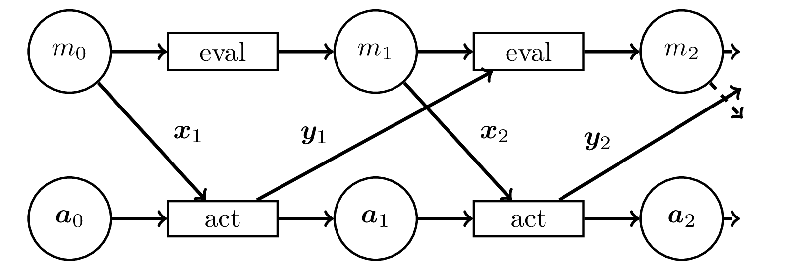
An experiment of ARL is the execution of this sequence. The resulting data of an experiment is the sequence of states, inputs and outputs $(m_{t},\bm{a}_{t},\bm{x_{t}},\bm{y}_{t}),t\in\{1,…,n\}$ as well as the initial setup $m_{0},\bm{a}_{0}$.

Thus finally we can strive to formalise the idea by collecting all components in a single scenario:

Definition 3.3 (Adversarial Resilience Learning Scenario).

Any experimental setup comprised of agent instances $a$ of $\mathcal{A}$ of two opposing classes $\mathcal{A}_{A}$ and $\mathcal{A}_{\Omega}$ and a system model $\mathcal{M}$, as well as, for each agent instance $a$ a reward function $p_{a}(m,t)$, a mapping of observable states $\bm{x}_{a,t}$, and action vectors $\bm{y}_{a,t}$.

ARL thus is the application of RL, as introduced in Section 2.2, to iteratively improve the internal decision structure that determines the behaviour of an agent $act_{a}$. The output of ARL then is, depending on the exerimenters objectives, an observation of the performance of the system model $\mathcal{M}$ or a set of agents trained towards the defined objectives.

3.3. Optimization Problem Statement

This section describes possible optimization problems that provide the motivation for ARL.

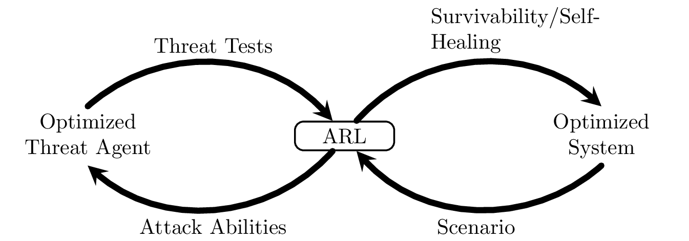
ARL resembles a closed-loop control situation with (at least) two conflicting controls. Herein are distinguished two different optimisation objectives that provide different uses of ARL. The different uses, as depicted in fig. 4, improve different elements to achive either an improved threat tests, or a more resilient system. The primary distinction is between evolving parameters of ANN in order to optimize individual agents or step-wise advancing the structure of the system model. Our concept itself is oblivious to the algorithms used for optimization.

Figure 4. Optimization Objectives

3.3.1. System Optimization

The primary objective is to find the inherent control asymmetry of a given control system to finally recommend system designs that favor the defender over the attacker. In control theory this could be expressed as a system, where for all possible sequences of actions by the attacker for a given system model $\mathcal{M}$ there is at least one corresponding sequence of actions for the defender and the resulting performance of the system will never drop below a given failure threshold. This requirement can be relaxed by defining a finite measure of failure that may be acceptable, for example during an initiation phase.

Objectives of defender and attacker in control scenarios are focussed on system states measured by a model performance function eq. 2, as formally given in definition 3.2. In general, we call an agent defender if its objective is to keep the performance at least above the failure threshold. We denote an agent as attacker if it aims at pushing the performance below a expression for a failure threshold, as seen in Figure 1.

We denote the objective of asymmetry — favouring defence of a system — given a candidate system model instance $m$ and defender agent $a_{\Omega}$ that

(8) $$p^{f}<p(m_{t})\text{ for all }t>t_{0},a_{A}\in A\leavevmode\nobreak\ .$$

Which describes that the performance, for all potential attackers $a$ in $A$, there exists a defender $a_{\Omega}^{*}$, with given initial state $m_{t_{0}}$, will never fall below a defined failure threshold $p^{f}$. To account for a learning period we allow for a finite initialisation time until $t_{0}$.

Improvement is achieved by evolutionary changes to the system model $\mathcal{M}$, improved defensive agent models $\mathcal{A}$ or training of defensive agents $a_{\Omega}$, as discussed in the following section.

3.3.2. Agent-Training

Training of threat agents aims at improving attack abilities, including the identification of previously unknown attack vectors, in order to provide testing capabilities. Improved threat tests allow to define test requirements for system designs that improve systems’ resilience against security threats. One objective is to train threat agents that can be used as benchmarks for future system designs.

An agent’s objective is implemented through a reward function that is used within a reinforcement learning process that successively improves the agent’s behaviour towards that objective.

One particularly surprising success of RLs algorithms has been the identification of solutions unthought-of by experts, especially if applied to zero-information initial states. A two-agent, conflicting-objectives game only one potential learning structure usable with ARL. But the concept allows potentially for all combinations of one-or-many zero-information reinforcment agents and static or even human-controlled competition.

4. Application to Power Systems

In this section an example application of ARL to adversarial control in power systems is shown as a feasibility demonstration. We show that ARL provides a novel approach to analyze fundamental control asymmetries between intelligent attackers and defenders. The final aim of this application is to design and analyse system configurations that are inherently favoring the defender in his objective to stabilize system performance.

Applied on power systems, e. g., the performance function is expressed as diversion from a specified range of acceptable state values. The attackers objective is to force the system to a state where one or more values are outside allowed ranges, its success is measured by the amount and duration of the deviation. The “defender” has lost the competition if the attacker is able to divert any of the system’s parameters beyond the acceptable range.

Specific objectives for attackers can vary widely as there are many different parts of a power system that can be affected in order to disrupt service and reduce system performance. Attackers may aim at demolition of connected machines or components of the transmission and control system. Thus, to strive for a more general specification of objectives, we better consider the objectives of defenders and specifiy a deviation from these objectives as “win” for the attackers. The objectives for the defender are very well defined in the power system domain.

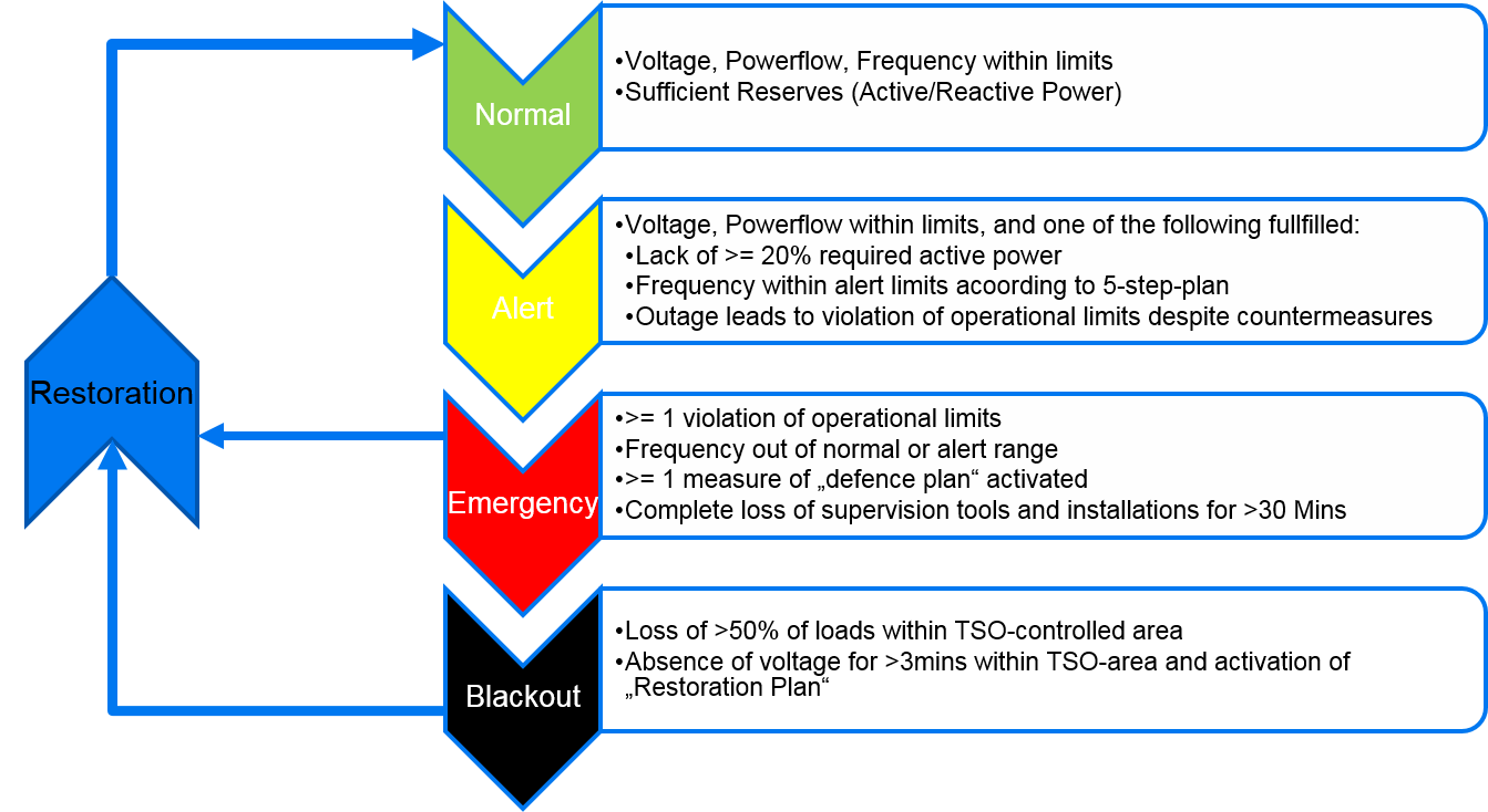
Different specific requirements apply for different parts of the power system. Common parameters to consider are voltage $V$ in $\mathrm{V}$, frequency $f$ in $\mathrm{H}\mathrm{z}$, phasor angle $\phi$ in $\mathrm{r}\mathrm{a}\mathrm{d}$, real power $P$ in $\mathrm{W}$, and reactive power in $\mathrm{V}\mathrm{A}\mathrm{r}$. In general, phase synchronicity is more important for high-voltage transmission grids, as asynchronicity leads to harmonics in the power system, with potentially desastreous large power flows between large segments of the grid. For the european transmission grid the operation guidelines, defining conditions for four phases: normal, alert, emergency, and blackout, shown in Figure 5, are defined in (tso, 2017).

Figure 5. ENTSO-E Operational Phases

Similarly operational parameters exist for medium- and low-voltage-grids, power generation and connected loads.

DIN EN 50160 specifies parameters for the operation of distribution grids. It defines that voltage has to stay between $0.9\text{\,}\mathrm{p}\mathrm{u}$ and $1.1\text{\,}\mathrm{p}\mathrm{u}$. It is acceptable, by definition in EN 50160, that voltage drops down to at least $0.85\text{\,}\mathrm{p}\mathrm{u}$ for at most 5% of a week. Frequency must only deviate from the nominal 50 Hz by at most 4% above or 6% for not more than 0.5% of the year, i. e., less than 2 days overall. Normal operation must deviate no more than $\pm 1$%. (Din, 2008)

An attack, in this simulation is deemed successful if any requirement exceeds its defined limits.

Figure 6. ARL ANN structure

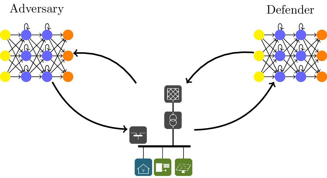
Figure 6 shows the refinement of the generic ARL-structure as described in section 3 for the power grid scenario using ANN to implement a single adversary and a single defender. Both agents interact only through sensors and actuators that influence different controls in the power grid.

In the remainder of this section we introduce a Proof-of-Concept (PoC) implementation of ARL using PandaPower (Thurner et al., 2018) for static grid simulation and the Keras-RL library (Plappert, 2016) for implementation of reinforcement learning for ANNs. First, a brief description of the control scenario is provided, followed by a discussion of the preliminary results.

4.1. Static Control Scenario

The objective of this proof-of-concept is to show the general feasibility of using (multiple) ANN-heuristics and train them by reinforcement learning to modify controls in a static power system simulation towards their objectives.

The simulation uses a simple medium voltage power grid, as model from the static grid simulation pandapower (Thurner et al., 2018). The grid contains four generators connected by six transformers to six loads. For the PoC, we chose to only use voltage as state-indicator and input to the reward of the attacker. The initial configuration of the grid comprises a stable healthy state of the grid that would be held up constantly if no control actions would be initiated.

Actuators in this scenario are tap changer, reactive power control, loads and generation levels as represented by the commonly deployed and future automated controls in power systems.

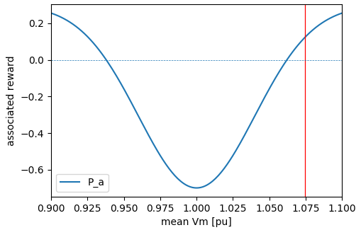
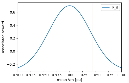
The reward function for the attacker is shown at the bottom right in Figure 9(a). Initial trials pointed towards the inverse of a Poisson Density Function centered on the nominal voltage unit. The reward function thus resembles the objective for an attacker, providing only positive rewards if the mean voltage deviates more than 5% from the nominal voltage. The single agent in this demonstration had been assigned direct control of every transformer, generator and load in this scenario.

In terms of optimization from Section 3.3, the scenario instantiates $m$ from $\mathcal{M}=\text{ Simple Example}$, with a single agent $a\in\mathcal{A}_{A}$, with a parametrized normal distribution

(9) $$p_{a}(m,t)={-1}^{[a\in\mathcal{A}_{\Omega}]}e^{-\frac{(x-\mu)^{2}}{2\sigma^{2}}}-c,$$

where $c,\mu$ and $\sigma$ parametrize the reward curve, ${-1}^{[a\notin\mathcal{A}_{A}]}$ negates the reward if $a$ is an attacker, and $x=\mathop{mean}{\bm{x}_{a,t}}$ is the average of all inputs.

4.2. Demonstrator

In order to show the genearal feasibility of the concept, we implemented a demonstrator for reinforcement learning in power control scenarios. The current implementation uses static simulation in PandaPower (Thurner et al., 2018). It supports free configurability of controlled sensors and actuators of multiple agents, selection of ANN-algorithms and -parameters, as well as different logging and output formats.

Each experiment is specified within a single configuration file, in order to support documentation and reproducibility of experiments. A experimental configuration (Figure 7) defines three major simulation components: a grid model, one or more agents, and a collection of result logs that collect results. At the time of writing, the whole demonstrator is refactored to use the mosaik co-simulation framework. (Schütte, 2013; Lehnhoff et al., 2015)

Figure 7. ARL Demonstrator configuration structure

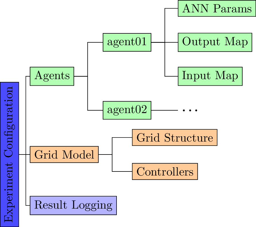
The interconnection between agents and grid simulation, i. e., the inputs (sensors) and outputs (actuators), $\bm{x}_{a}$ and $\bm{y}_{a}$ respectively, are separately defined for each agent.

The execution of the simulation is round based. The rounds are advanced in steps according to a defined evaluation order of agents. Agents are sequentially executed, a defined number of steps each. The grid state is evaluated between each consecutive pair of agent evaluation steps. After each step, the internal weights of an agent are modified by the learning algorithm selected in the configuration of an agent.

Current result monitors output the grid states at every node of the grid into a grid-state-log. For the agents, a log consisting of inputs, outputs and evaluated reward for the output is output to a configurable file in CSV format. The results are graphically evaluated as is discussed in Section 4.3 below.

4.3. Results

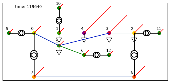
To show the usability of our demonstrator we pitched two very simplistic agents with inverse reward functions (Figure 9(a) and Figure 9(d)) against each other, using the example grid shown in Figure 8(a) as an arena. Both agents were assigned all voltage sensors as input and we divided the actuators among their outputs. The attacker was assigned control of all tab changers, representing a scenario where a vulnerability in one type of controller was exploited. The defender would be granted access to all generators and loads in this scenario.

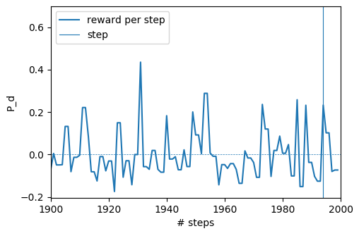
Figure 8 shows a late state of the simulation. Seemingly the attacker gained the upper hand and has been able to increase voltage levels beyond 1.05 pu. The grid representation in Figure 8(a) shows that especially two central measure points (numbered 4 and 3) are struck with very high voltage levels, represented by the length of the bars rooted at the nodes, most likely sufficent for the connected loads to shut down or be damaged. The mean voltage level of the system, depicted for steps 1900 until 2000, in Figure 8(b) shows that even the lower voltages of other nodes, e. g., 11 and 9 are not sufficient to lower the mean voltage to acceptable levels. Thus, in this example the attacker has been able to destabilize the grid, despite the efforts of the attacker.

(a) Grid Simulation

(b) Grid performance (mean voltage) over time/evaluation steps

Figure 8. Proof-of-concept ARL grid results

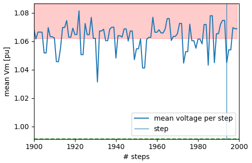
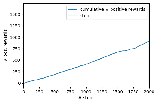
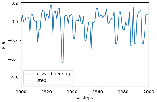
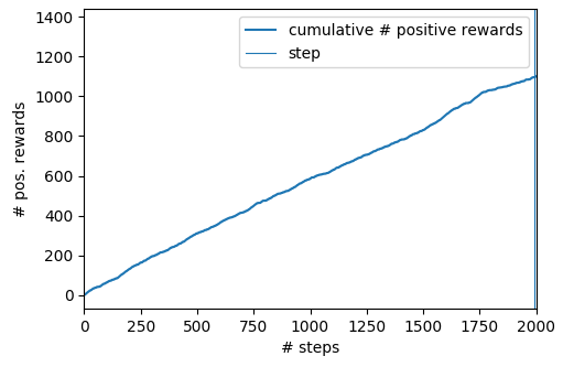
Evaluating the two agents in Section 3.1 provides no immediately conclussive cause for the loss of the defender. The cumulative number of positive rewards in Figure 9(b) for the attacker and Figure 9(e), show only small differences. These asymmetries might be explained by the order of execution, where the defender always acts in response to the attacker. The current reward for the depicted step in the simulation, depicted in Figure 9(a) and Figure 9(d), shows that the defender is evaluating a different mean voltage than the attacker. Each reward is calculated after the actions of an agent, thus this graphs show the results of two actions that both improved the performance towards their own objectives.

In this simulation run, that contained a small random input to the learning algorithm, the positive learning curve for both agents, in Figure 9(b) and Figure 9(e), is increasing right from the start of the simulation. In preliminary tests with a lone attacker, the learning process first went through a lengthy phase where only little positive rewards where achieved. Although we have no conclussive answer for the reasons of this diverging learning behaviour, it shows at least, that the interactions between adversaries have an effect on their behaviour.

(a) Attacker reward function, based on mean voltage

(b) Cumulative number of positive rewards over training steps

(c) Attacker performance $p_{a}(m_{t})$ over time (inverse mean voltage)

(d) Defender reward function, based on mean voltage

(e) Cumulative number of positive rewards over training steps

(f) Defender performance $p_{a}(t)$ over time (mean voltage)

Figure 9. Proof-of-concept ARL agent results

5. Discussion and Future Work

color=orange!40]LaF: Non-commutative application of actions

This work introduced Adversarial Resilience Learning (ARL), a novel approach to analyse competetive situations in highly-complex systems using reinforcement learning with artificial neural networks as reproducable, self-improving agents. The concept can be seen as an extension of Generative Adversarial Network (GAN), which distinguishes itself by including interaction to a complex system (simulation) in between the competing agents. This work is motivated by the need to find better methods to automatically evaluate system behaviour under threat of maliciously acting, intelligent threat agents. The main idea is, that groups of agents, modelled by Artificial Neural Network (ANN), struggle to enforce their objectives against agents with conflicting objectives.

Pitching two—or more—ANNs with conflicting reward functions against each other may allow to define more realistic tests for adversarial or competitive situations. Using reinforcement learning harbours the promise of finding novel strategies for both attack and defense, which both can be used to strengthen the resilience of systems during the design and testing phase of a power system or individual components. ARL-based analysis should contribute to building grid structures that are more resilient to attacks and train both artificial and human operators in better handling of security incidents.

Generally, the concept may allow to estimate threat-related indices, for example the maximum amount of control that an adversary may be allowed to gain over a system, which leads to improved and more effective recommendations for security directives and risk mitigations.

Furthermore, we believe that ARL provides a valuable addition to the increased complexity for adversarial learning. Agents in ARL have not only to approximate the behaviour of a highly-complex systsem, but also have to learn and adopt to changing behaviour of this system due to the actions inflicted by the competing agents. In this way, not only the amount of control over a system provides a source of asymmetry, but also power of the ANN.

The concept of ARL and its ongoing implementation in the ARL-Demonstrator only marks the starting point for in-depth research on structural asymmetries of complex systems and protection against learning threat agents. The demonstrator provides the abilities to further research in a number of interesting directions.

Foremost is the analysis of structural resilience of complex systems, especially finding minimum control sets of critical components that provide the most defensive capabilities, or estimates of the structural strength of a system. The integration into our co-simulation framework mosaik opens up the possibility of extending the single system into a whole composition into an interdependent system-of-systems. Introduction of multiple domains would, to give one example, allow to analyse the effects of Information and Communication Technology (ICT)-components onto the performance of power systems.

Deeper extensions of the demonstrator itself will involve capabilities of the defender to affect structural changes to the system. This would allow to use Reinforcement Learning (RL) to identify novel and more resilient structures. The dual ability for threat agents would be the extension of control, i. e., simulation of further compromise from within a system. Both activities require the introduction of a measure of cost to the demonstrator.

This demonstrator further allows to analyse simulated systems from the point of view of threat agents, by pitching the agent against novel security measures, for example simulation of distributed coordinated attacks. Combining this view with multi-domain scenarios, would enable analysis of sophisticated, multi-level attack techniques that involve, for example information hiding or emission of misleading information by attacker or defender. That means finding novel ways of attack using a combination of illeagal and legal operations and interdependencies between different systems. Consequentially all these approaches would lead to the development of improved designs and testing methods for highly complex systems.

We can only assume that this finally lead to more resilient designs and defensive adaptable strategies — and, in the end, to improvements for the security of supply, but at this stage of the work, the first results are very satisfying.

References

- (1)
- tso (2017) 2017. COMMISSION REGULATION (EU) 2017/1485 of 2 August 2017 establishing a guideline on electricity transmission system operation. Official Journal of the European Union L 220 (2017), 120. https://eur-lex.europa.eu/legal-content/EN/TXT/?uri=uriserv:OJ.L_.2017.220.01.0001.01.ENG&toc=OJ:L:2017:220:TOC Operation Guidelines.
- Arghandeh et al. (2016) Reza Arghandeh, Alexandra Von Meier, Laura Mehrmanesh, and Lamine Mili. 2016. On the definition of cyber-physical resilience in power systems. Renewable and Sustainable Energy Reviews 58 (may 2016), 1060–1069. https://doi.org/10.1016/j.rser.2015.12.193 arXiv:1504.05916
- Basharat and Shah (2009) A. Basharat and M. Shah. 2009. Time series prediction by chaotic modeling of nonlinear dynamical systems. In 2009 IEEE 12th International Conference on Computer Vision. 1941–1948. https://doi.org/10.1109/ICCV.2009.5459429
- Brown et al. (2006) Gerald Brown, Matthew Carlyle, Javier SalmerÃf³n, and Kevin Wood. 2006. Defending Critical Infrastructure. Interfaces 36, 6 (2006), 530 – 544. http://search.ebscohost.com.proxy02a.bis.uni-oldenburg.de/login.aspx?direct=true&db=buh&AN=23639043&site=ehost-live
- Cessac (2010) Bruno Cessac. 2010. A view of neural networks as dynamical systems. International Journal of Bifurcation and Chaos 20, 06 (2010), 1585–1629.
- Cho et al. (2014) Kyunghyun Cho, Bart Van Merriënboer, Caglar Gulcehre, Dzmitry Bahdanau, Fethi Bougares, Holger Schwenk, and Yoshua Bengio. 2014. Learning phrase representations using RNN encoder-decoder for statistical machine translation. arXiv preprint arXiv:1406.1078 (2014).
- Chung et al. (2014) Junyoung Chung, Caglar Gulcehre, KyungHyun Cho, and Yoshua Bengio. 2014. Empirical evaluation of gated recurrent neural networks on sequence modeling. arXiv preprint arXiv:1412.3555 (2014).
- Cuéllar et al. (2007) Manuel P Cuéllar, Miguel Delgado, and MC Pegalajar. 2007. An application of non-linear programming to train recurrent neural networks in time series prediction problems. In Enterprise Information Systems VII. Springer, 95–102.
- Cybenko (1989) George Cybenko. 1989. Approximation by superpositions of a sigmoidal function. Mathematics of control, signals and systems 2, 4 (1989), 303–314.
- Din (2008) En Din. 2008. DIN EN 50160: 2000-03 Merkmale der Spannung in öffentlichen Elektrizitätsversorgungsnetzen. Berlin: Beuth (2008).
- Do et al. (2017) Cuong T. Do, Nguyen H. Tran, Choongseon Hong, Charles A. Kamhoua, Kevin A. Kwiat, Erik Blasch, Shaolei Ren, Niki Pissinou, and Sundaraja Sitharama Iyengar. 2017. Game Theory for Cyber Security and Privacy. ACM Comput. Surv. 50, 2, Article 30 (may 2017), 37 pages. https://doi.org/10.1145/3057268
- Dozat (2016) Timothy Dozat. 2016. Incorporating nesterov momentum into adam. (2016).
- Elman (1990) Jeffrey L Elman. 1990. Finding structure in time. Cognitive science 14, 2 (1990), 179–211.
- Ernst et al. (2004) D. Ernst, M. Glavic, and L. Wehenkel. 2004. Power systems stability control: reinforcement learning framework. IEEE Transactions on Power Systems 19, 1 (feb 2004), 427–435. https://doi.org/10.1109/TPWRS.2003.821457
- Evtimov et al. (2017) Ivan Evtimov, Kevin Eykholt, Earlence Fernandes, Tadayoshi Kohno, Bo Li, Atul Prakash, Amir Rahmati, and Dawn Song. 2017. Robust Physical-World Attacks on Deep Learning Models. arXiv preprint arXiv:1707.08945 1 (2017).
- Ghahramani (2004) Zoubin Ghahramani. 2004. Unsupervised learning. In Advanced lectures on machine learning. Springer, 72–112.
- Goodfellow et al. (2016) Ian Goodfellow, Yoshua Bengio, Aaron Courville, and Yoshua Bengio. 2016. Deep learning. Vol. 1. MIT press Cambridge.
- Goodfellow et al. (2014) Ian Goodfellow, Jean Pouget-Abadie, Mehdi Mirza, Bing Xu, David Warde-Farley, Sherjil Ozair, Aaron Courville, and Yoshua Bengio. 2014. Generative adversarial nets. In Advances in neural information processing systems. 2672–2680.
- Goodfellow et al. (2015) Ian J. Goodfellow, Jonathon Shlens, and Christian Szegedy. 2015. Explaining and Harnessing Adversarial Examples. https://arxiv.org/abs/1412.6572
- Graves et al. (2014) Alex Graves, Greg Wayne, and Ivo Danihelka. 2014. Neural turing machines. arXiv preprint arXiv:1410.5401 (2014).
- Hansen (2006) Nikolaus Hansen. 2006. The CMA evolution strategy: a comparing review. In Towards a new evolutionary computation. Springer, 75–102.
- Hansen et al. (2003) Nikolaus Hansen, Sibylle D Müller, and Petros Koumoutsakos. 2003. Reducing the time complexity of the derandomized evolution strategy with covariance matrix adaptation (CMA-ES). Evolutionary computation 11, 1 (2003), 1–18.
- Hochreiter and Schmidhuber (1997) Sepp Hochreiter and Jürgen Schmidhuber. 1997. Long short-term memory. Neural computation 9, 8 (1997), 1735–1780.
- Hornik et al. (1989) Kurt Hornik, Maxwell Stinchcombe, and Halbert White. 1989. Multilayer feedforward networks are universal approximators. Neural networks 2, 5 (1989), 359–366.
- III (1994) Leemon C. Baird III. 1994. Reinforcement Learning in Continuous Time: Advance Updating. In IEEE World Congress on Computational Intelligence, 1994 IEEE International Conference on Neural Networks.
- Isaacs (1965) Rufus Isaacs. 1965. Differential games: a mathematical theory with applications to warfare and pursuit, control and optimization. John Wiley and Sons.
- Iverson (1962) Kenneth E. Iverson. 1962. A Programming Language. In Proceedings of the May 1-3, 1962, Spring Joint Computer Conference (AIEE-IRE ’62 (Spring)). ACM, New York, NY, USA, 345–351. https://doi.org/10.1145/1460833.1460872
- Kingma and Ba (2014) Diederik P Kingma and Jimmy Ba. 2014. Adam: A method for stochastic optimization. arXiv preprint arXiv:1412.6980 (2014).
- Lehnhoff et al. (2015) Sebastian Lehnhoff, Okko Nannen, Sebastian Rohjans, Florian Schlogl, Stefan Dalhues, Lena Robitzky, Ulf Häger, and Christian Rehtanz. 2015. Exchangeability of power flow simulators in smart grid co-simulations with mosaik. In 2015 Workshop on Modeling and Simulation of Cyber-Physical Energy Systems, MSCPES. https://doi.org/10.1109/MSCPES.2015.7115410
- Linkov and Kott (2019) Igor Linkov and Alexander Kott. 2019. Fundamental Concepts of Cyber Resilience: Introduction and Overview. Springer International Publishing, Cham, 1–25. https://doi.org/10.1007/978-3-319-77492-3_1
- Minsky (1954) Marvin Minsky. 1954. Neural nets and the brain-model problem. Unpublished doctoral dissertation, Princeton University, NJ (1954).
- Plappert (2016) Matthias Plappert. 2016. keras-rl. https://github.com/keras-rl/keras-rl.
- Ros and Hansen (2008) Raymond Ros and Nikolaus Hansen. 2008. A simple modification in CMA-ES achieving linear time and space complexity. In International Conference on Parallel Problem Solving from Nature. Springer, 296–305.
- Ruder (2016) Sebastian Ruder. 2016. An overview of gradient descent optimization algorithms. arXiv preprint arXiv:1609.04747 (2016).
- Rumelhart et al. (1986) David E Rumelhart, Geoffrey E Hinton, and Ronald J Williams. 1986. Learning representations by back-propagating errors. nature 323, 6088 (1986), 533.
- Ruppert et al. (2014) Martin Ruppert, Eric MSP Veith, and Bernd Steinbach. 2014. An Evolutionary Training Algorithm for Artificial Neural Networks with Dynamic Offspring Spread and Implicit Gradient Information. In Proceedings of the Sixth International Conference on Emerging Network Intelligence (EMERGING 2014). Rome, Italy: International Academy, Research, and Industry Association. Citeseer.
- Schütte (2013) Steffen Schütte. 2013. Simulation Model Composition for the Large-Scale Analysis of Smart Grid Control Mechanisms. PhD. Carl von Ossietzky University of Oldenburg. http://oops.uni-oldenburg.de/1768/
- Seidl and Lorenz (1991) D. R. Seidl and R. D. Lorenz. 1991. A structure by which a recurrent neural network can approximate a nonlinear dynamic system. In IJCNN-91-Seattle International Joint Conference on Neural Networks, Vol. ii. 709–714 vol.2. https://doi.org/10.1109/IJCNN.1991.155422
- Siegelmann and Sontag (1995) Hava T Siegelmann and Eduardo D Sontag. 1995. On the computational power of neural nets. Journal of computer and system sciences 50, 1 (1995), 132–150.
- Silver et al. ([n. d.]) David Silver, Julian Schrittwieser, Karen Simonyan, Ioannis Antonoglou, Aja Huang, Arthur Guez, Thomas Hubert, Lucas Baker, Matthew Lai, Adrian Bolton, Yutian Chen, Timothy Lillicrap, Fan Hui, Laurent Sifre, George van den Driessche, Thore Graepel, and Demis Hassabis. [n. d.]. Mastering the game of Go without human knowledge. 550 ([n. d.]), 354. http://dx.doi.org/10.1038/nature24270
- Thurner et al. (2018) L. Thurner, A. Scheidler, F. Schafer, J. H. Menke, J. Dollichon, F. Meier, S. Meinecke, and M. Braun. 2018. pandapower - an Open Source Python Tool for Convenient Modeling, Analysis and Optimization of Electric Power Systems. IEEE Transactions on Power Systems (2018). https://doi.org/10.1109/TPWRS.2018.2829021
- Tong (1990) Howell Tong. 1990. Non-linear time series: a dynamical system approach. Oxford University Press.
- Veith (2017) Eric MSP Veith. 2017. Universal Smart Grid Agent for Distributed Power Generation Management. Logos Verlag Berlin GmbH, Chapter Forecasting Power Demand and Supply, 100–108.
- Yu et al. (2007) Wenwu Yu, Guanrong Chen, Jinde Cao, Jinhu Lü, and Ulrich Parlitz. 2007. Parameter identification of dynamical systems from time series. Physical Review E 75, 6 (2007), 067201.