Learning to Bound the Multi-class Bayes Error

Salimeh Yasaei Sekeh∗†, Member, IEEE, Brandon Oselio, Member, IEEE,
 Alfred O. Hero, Fellow, IEEE 
Department of EECS, University of Michigan, Ann Arbor, MI, USA
School of Computing and Information Science, University of Maine, Orono, ME, USA
The work presented in this paper was partially supported by ARO grant W911NF-15-1-0479 and DOE grant DE-NA0002534. The authors also acknowledge support from AFRL under grant USAF FA8650-15-D-1845. Some parts of this paper have been presented at the Annual Allerton Conference on Communication, Control, and Computing, 2018.
Abstract

In the context of supervised learning, meta learning uses features, metadata and other information to learn about the difficulty, behavior, or composition of the problem. Using this knowledge can be useful to contextualize classifier results or allow for targeted decisions about future data sampling. In this paper, we are specifically interested in learning the Bayes error rate (BER) based on a labeled data sample. Providing a tight bound on the BER that is also feasible to estimate has been a challenge. Previous work [1] has shown that a pairwise bound based on the sum of Henze-Penrose (HP) divergence over label pairs can be directly estimated using a sum of Friedman-Rafsky (FR) multivariate run test statistics. However, in situations in which the dataset and number of classes are large, this bound is computationally infeasible to calculate and may not be tight. Other multi-class bounds also suffer from computationally complex estimation procedures. In this paper, we present a generalized HP divergence measure that allows us to estimate the Bayes error rate with log-linear computation. We prove that the proposed bound is tighter than both the pairwise method and a bound proposed by Lin [2]. We also empirically show that these bounds are close to the BER. We illustrate the proposed method on the MNIST dataset, and show its utility for the evaluation of feature reduction strategies. We further demonstrate an approach for evaluation of deep learning architectures using the proposed bounds.

Index Terms:
meta learning, multi-class classification, Henze-Penrose divergence, Bayes error rate, Friedman-Rafsky statistic, minimal spanning tree.

I Introduction

Meta-learning is a method for learning the intrinsic quality of data directly from a sample of the data, metadata, or other information [3], [4]. The purpose of meta-learning is to collect knowledge that might be helpful at other levels of processing and decision-making. Examples where meta-learning is applied include sequential design of experiments [5], reinforcement learning [6], and sensor management [7] in the fields of statistics, machine learning, and systems engineering, respectively. In supervised learning, and particularly for multi-class classification, one form of meta-learning is to learn bounds or estimates on the Bayes error rate (BER). The BER is the minimal achievable error probability of any classifier for the particular learning problem, and knowledge of it can be used at other stages of meta-learning, such as in the selection of the classifiers, model selection, and feature reduction. Hence, finding computable bounds and approximations to the BER is of interest, and is the problem we consider in this paper.

Consider the problem where a feature vector 𝐗𝐗\mathbf{X} is labeled over m𝑚m classes C1,,Cmsubscript𝐶1subscript𝐶𝑚C_{1},\ldots,C_{m}. Available are i.i.d. pairs {(𝐱i,yi)}i=1nsuperscriptsubscriptsubscript𝐱𝑖subscript𝑦𝑖𝑖1𝑛\{(\mathbf{x}_{i},y_{i})\}_{i=1}^{n}, called training data, where 𝐱isubscript𝐱𝑖\mathbf{x}_{i} is a realization of the random vector (feature) 𝐗d𝐗superscript𝑑\mathbf{X}\in\mathbb{R}^{d} and yisubscript𝑦𝑖y_{i} is a realization of the random variable (label) Y{1,2,,m}𝑌12𝑚Y\in\{1,2,\dots,m\}. Assume the prior label probabilities pk=P(Y=k)subscript𝑝𝑘𝑃𝑌𝑘p_{k}=P(Y=k), with k=1mpk=1superscriptsubscript𝑘1𝑚subscript𝑝𝑘1\displaystyle\sum\limits_{k=1}^{m}p_{k}=1 and the conditional feature densities fk(𝐱)=f(𝐱|Y=k)subscript𝑓𝑘𝐱𝑓conditional𝐱𝑌𝑘f_{k}(\mathbf{x})=f(\mathbf{x}|Y=k), for k=1,,m𝑘1𝑚k=1,\dots,m. Then the Bayes error rate is given by

ϵm=1max{p1f1(𝐱),p2f2(𝐱),,pmfm(𝐱)}d𝐱.superscriptitalic-ϵ𝑚1subscript𝑝1subscript𝑓1𝐱subscript𝑝2subscript𝑓2𝐱subscript𝑝𝑚subscript𝑓𝑚𝐱differential-d𝐱\epsilon^{m}=1-\displaystyle\int\max\{p_{1}f_{1}(\mathbf{x}),p_{2}f_{2}(\mathbf{x}),\dots,p_{m}f_{m}(\mathbf{x})\}\;\rm{d}\mathbf{x}. (1)

This represents the error achieved by the Bayes classifier, gBayessubscript𝑔𝐵𝑎𝑦𝑒𝑠g_{Bayes} that minimizes the average 01010-1 loss. The Bayes classifier assigns an estimated class label y^^𝑦\hat{y} to an observation 𝐱𝐱\mathbf{x} according to the maximum a posterior (MAP) rule

y^=gBayes(𝐱)=argmaxk{1,2,,m}P(Y=k|𝐗=𝐱).^𝑦subscript𝑔𝐵𝑎𝑦𝑒𝑠𝐱subscriptargmax𝑘12𝑚𝑃𝑌conditional𝑘𝐗𝐱\hat{y}=g_{Bayes}(\mathbf{x})=\operatorname*{arg\,max}_{k\in\{1,2,\ldots,m\}}P(Y=k|\mathbf{X}=\mathbf{x}).

Many different upper and lower bounds on the BER (1) exist for the case of m=2𝑚2m=2 classes, and many of these are related to the family of f𝑓f-divergences. A bound based on Chernoff α𝛼\alpha-divergence has been proposed in [8], but in general it is not very tight in the finite sample regime. In [9], a tighter bound for the 2-class BER using Henze-Penrose [10] divergence was proposed. The HP bound has the advantage that it can be directly estimated from the training data using a minimal spanning tree. The same framework can be extended in a pairwise fashion to the m𝑚m-class multi-class classification problem. However, when m𝑚m is relatively large, the derived pairwise bounds are loose and often times trivial [11]. The method proposed in this paper alleviates this problem by introducing new bounds based on a generalized Henze-Penrose measure adapted to m𝑚m-class problem, and whose tightness does not diminish as m𝑚m increases. Additionally, the new bounds improve upon other bounds that were designed specifically for the multi-class problem, such as the generalized Jensen-Shannon (JS) divergence bound [2].

Most approaches to estimation of bounds on Bayes error use plug-in estimators. These approaches require estimation of the multivariate feature densities followed by evaluation of the BER bounds using these estimated densities in place of the true densities. Recently, approaches to estimating BER bounds using direct estimators have been proposed. For example, graph-based BER bound estimation approaches bypass density estimation entirely, producing an estimator of the information divergence using geometric functions of the data. These procedures scale linearly in dimension, resulting in faster computation than plug-in methods for high dimensional features. In the original 2-class setting, as shown in [9], bounds based on Henze-Penrose divergence can be estimated directly from data by employing the Friedman-Rafsky (FR) run test statistic [12, 10], which computes a minimal spanning tree (MST) over the data, and counts the number of edges that connect dichotomous data points. A brute force extension of the FR approach to the m𝑚m-class classification problem would require an MST computation for each pair of classes, or O(m2)𝑂superscript𝑚2O(m^{2}) MSTs, which significantly reduces its computational tractability for large m𝑚m. The extension proposed in this paper also uses a graph-based estimation procedure, but only requires a single MST calculation on the entire dataset. Thus, the proposed approach is more computationally efficient when m𝑚m and n𝑛n are large.

I-A Related Work

Broadly defined, meta-learning is a set of methods of learning from knowledge that can be used to improve performance or understanding of the problem. Estimating the Bayes multi-class classification error is a meta-learning problem. The principles behind the frameworks proposed in [13] and [14] have been utilized to estimate the multi-class BER by bounding the BER by a sum of pairwise BERs for each pair of class labels. There exist many useful bounds on the pairwise BER that are based on information divergence measures, i.e., measures of dissimilarity between two distributions. Several bounds for the pairwise BER have been proposed, including: Chernoff bound [8]; Bhattacharyya bound [15]; and HP-divergence [9]. The Henze-Penrose divergence yields tighter bounds on the BER than those based on the Bhattacharya distance for equal label priors. For the multi-class BER, the sum of pairwise bounds given in [1] was proposed.

Another approach to bounding the BER of multi-class classifiers uses the Jensen-Shannon (JS) divergence. The JS-divergence assigns a different weight to each conditional probability distribution and this inspired Lin to propose a bound for the binary BER where the weights depend on the priors. The generalized multi-class Jensen-Shannon divergence is related to the Jensen difference proposed by Rao [16, 17]. In [2], the author proposed a generalized JS-divergence that was used to derive a bound on the Bayes error rate for multi-class classification.

In the nonparametric setting, the most popular approach for estimating bounds has been plug-in estimators, which require estimation of probability densities that are subsequently “plugged into” the expression for the divergence function, [18, 19, 20]. These approaches are generally multi-step procedures and computationally expensive, especially in high dimensions [21]. In [22], Nguyen et al. proposed a divergence estimation method based on estimating the likelihood ratio of two densities that achieves the parametric mean squared error (MSE) convergence rate when the densities are sufficiently smooth.

Direct estimation approaches bypass density estimation, producing an estimator of the information divergence using geometric functions of the data. As previously mentioned, the MST-based Friedman-Rafsky two sample test statistic [12, 10] is an asymptotically consistent estimator of the HP-divergence, which can then be used to estimate upper and lower bounds for the 2-class classification problem [9]. There are other graph-based estimators that have been proposed in the literature. The author in [23] proposed a graph-based estimator for HP-divergence that employs the K-nearest neighbor (K-NN) graph instead of the MST. The authors of [24] developed an approach for estimating general f𝑓f-divergences called the Nearest Neighbor Ratio (NNR), also using K-NN graphs. In [25] the authors developed a general divergence estimator based on Locality Sensitive Hashing (LSH). In [26], the authors showed that a cross match statistic based on optimal weighted matching can also be used to directly estimate the HP divergence. None of these papers on geometric methods proposed extensions to multi-class classification, which is the main contribution of this paper.

I-B Contribution

We introduce a computationally scalable and statistically consistent method for learning to bound the multi-class BER. First, we propose a novel measure, the generalized Henze-Penrose (GHP) integral, for bounding multi-class BER. We show how this generalized integral can be used to calculate bounds on the Bayes error rate, and prove that they are tighter than both the pairwise and JS multi-class BER bounds. Further, we empirically show that the bounds’ performance is consistent and is robust to sample size and the number of classes.

Our second contribution is a scalable method for estimating the GHP integral, and subsequent estimation of the BER bounds. The proposed algorithm uses a single global minimal spanning tree (MST) constructed over the entire dataset. We show that this is more computationally efficient than the pairwise approach, which must compute O(m2)𝑂superscript𝑚2O(m^{2}) pairwise MSTs.

I-C Organization of the paper

The paper is organized as follows. In Section II-A we briefly review the HP divergence and propose the generalized HP-integral (GHP) measure. The motivation and theory for the various bounds such as the pairwise HP divergence and generalized JS divergence for the multi-class Bayes error is reviewed in Section III, and a new bound based on our GHP measure is given. We numerically illustrate the theory in Section V. In Section VI we apply the proposed method to a real dataset, the MNIST image dataset. Finally, Section VII concludes the paper. The main proofs of the theorems in the paper are given in the longer version of the paper on arXiv.

II The Divergence Measure and Generalizations

In this section we recall the Henze-Penrose (HP) divergence between pairs of densities and define a generalization for multiple densities (2absent2\geq 2) that will be the basis for learning to bound multi-class BER, called "Generalized HP-integral".

II-A Henze-Penrose Divergence

For parameters p(0,1)𝑝01p\in(0,1) and q=1p𝑞1𝑝q=1-p consider two density functions f𝑓f and g𝑔g with common domain dsuperscript𝑑\mathbb{R}^{d}. The Henze-Penrose divergence D(f,g)𝐷𝑓𝑔D(f,g) is given by

D(f,g)=14pq[(pf(𝐱)qg(𝐱))2pf(𝐱)+qg(𝐱)d𝐱(pq)2].𝐷𝑓𝑔14𝑝𝑞delimited-[]superscript𝑝𝑓𝐱𝑞𝑔𝐱2𝑝𝑓𝐱𝑞𝑔𝐱differential-d𝐱superscript𝑝𝑞2D(f,g)=\displaystyle\frac{1}{4pq}\left[\int\displaystyle\frac{\big{(}pf(\mathbf{x})-qg(\mathbf{x})\big{)}^{2}}{pf(\mathbf{x})+qg(\mathbf{x})}\;{\rm d}\mathbf{x}-(p-q)^{2}\right]. (2)

The HP-divergence (2), first introduced in [27], has the following properties: (1) 0D10𝐷10\leq D\leq 1, (2) D=0𝐷0D=0 iff f(𝐱)=g(𝐱)𝑓𝐱𝑔𝐱f(\mathbf{x})=g(\mathbf{x}). Note that the HP-divergence belongs to the f𝑓f-divergence family [28, 29, 30].

In the multi-class classification setting, as defined in the introduction, consider a sample of i.i.d. pairs (𝐱i,yi)subscript𝐱𝑖subscript𝑦𝑖(\mathbf{x}_{i},y_{i}), i=1,,n𝑖1𝑛i=1,\ldots,n, where yi{1,,m}subscript𝑦𝑖1𝑚y_{i}\in\{1,\ldots,m\} are class labels with prior probabilities {pk}k=1msuperscriptsubscriptsubscript𝑝𝑘𝑘1𝑚\{p_{k}\}_{k=1}^{m} and, given yi=ksubscript𝑦𝑖𝑘y_{i}=k, 𝐱isubscript𝐱𝑖\mathbf{x}_{i} has conditional density fksubscript𝑓𝑘f_{k}. Define p~ij=pi/(pi+pj)subscript~𝑝𝑖𝑗subscript𝑝𝑖subscript𝑝𝑖subscript𝑝𝑗\widetilde{p}_{ij}=p_{i}/(p_{i}+p_{j}). Note that p~ijp~jisubscript~𝑝𝑖𝑗subscript~𝑝𝑗𝑖\widetilde{p}_{ij}\neq\widetilde{p}_{ji} and p~ij+p~ji=1subscript~𝑝𝑖𝑗subscript~𝑝𝑗𝑖1\widetilde{p}_{ij}+\widetilde{p}_{ji}=1. Let 𝕊(i)superscript𝕊𝑖\mathbb{S}^{(i)} be the support set of the conditional distribution fisubscript𝑓𝑖f_{i}. The Henze-Penrose (HP) divergence measure between distributions fisubscript𝑓𝑖f_{i} and fjsubscript𝑓𝑗f_{j} with union domain 𝕊(ij)=𝕊(i)𝕊(j)superscript𝕊𝑖𝑗superscript𝕊𝑖superscript𝕊𝑗\mathbb{S}^{(ij)}=\mathbb{S}^{(i)}\cup\mathbb{S}^{(j)} is defined as follows (see [10, 27, 9]):

D(fi,fj)𝐷subscript𝑓𝑖subscript𝑓𝑗\displaystyle D(f_{i},f_{j})
=14p~ijp~ji[𝕊(ij)(p~ijfi(𝐱)p~jifj(𝐱))2p~ijfi(𝐱)+p~jifj(𝐱)d𝐱(p~𝑖𝑗p~𝑗𝑖)2].absent14subscript~𝑝𝑖𝑗subscript~𝑝𝑗𝑖delimited-[]subscriptsuperscript𝕊𝑖𝑗superscriptsubscript~𝑝𝑖𝑗subscript𝑓𝑖𝐱subscript~𝑝𝑗𝑖subscript𝑓𝑗𝐱2subscript~𝑝𝑖𝑗subscript𝑓𝑖𝐱subscript~𝑝𝑗𝑖subscript𝑓𝑗𝐱differential-d𝐱superscriptsubscript~𝑝𝑖𝑗subscript~𝑝𝑗𝑖2\displaystyle\quad=\displaystyle\frac{1}{4\widetilde{p}_{ij}\widetilde{p}_{ji}}\Big{[}\int_{\mathbb{S}^{(ij)}}\frac{\big{(}\widetilde{p}_{ij}f_{i}(\mathbf{x})-\widetilde{p}_{ji}f_{j}(\mathbf{x})\big{)}^{2}}{\widetilde{p}_{ij}f_{i}(\mathbf{x})+\widetilde{p}_{ji}f_{j}(\mathbf{x})}\;\rm{d}\mathbf{x}-({\it\widetilde{p}_{ij}-\widetilde{p}_{ji})}^{2}\Big{]}. (3)

An alternative form for D(fi,fj)𝐷subscript𝑓𝑖subscript𝑓𝑗D(f_{i},f_{j}) is given in terms of the HP-integral:

HPij:=HP(fi,fj)=𝕊(ij)fi(𝐱)fj(𝐱)pifi(𝐱)+pjfj(𝐱)d𝐱,assignsubscriptHP𝑖𝑗HPsubscript𝑓𝑖subscript𝑓𝑗subscriptsuperscript𝕊𝑖𝑗subscript𝑓𝑖𝐱subscript𝑓𝑗𝐱subscript𝑝𝑖subscript𝑓𝑖𝐱subscript𝑝𝑗subscript𝑓𝑗𝐱differential-d𝐱{\rm HP}_{ij}:={\rm HP}\big{(}f_{i},f_{j}\big{)}=\int_{\mathbb{S}^{(ij)}}\displaystyle\frac{f_{i}(\mathbf{x})f_{j}(\mathbf{x})}{p_{i}f_{i}(\mathbf{x})+p_{j}f_{j}(\mathbf{x})}\rm{d}\mathbf{x}, (4)

yielding the equivalent form to (II-A)

D(fi,fj)=1(pi+pj)HPij.𝐷subscript𝑓𝑖subscript𝑓𝑗1subscript𝑝𝑖subscript𝑝𝑗subscriptHP𝑖𝑗D(f_{i},f_{j})=1-(p_{i}+p_{j}){\rm HP}_{ij}.

In [9] it was shown that 0D(fi,fj)10𝐷subscript𝑓𝑖subscript𝑓𝑗10\leq D(f_{i},f_{j})\leq 1, and that the HP-integral is upper bounded by HP(fi,fj)(pi+pj)1HPsubscript𝑓𝑖subscript𝑓𝑗superscriptsubscript𝑝𝑖subscript𝑝𝑗1{\rm HP}\big{(}f_{i},f_{j}\big{)}\leq(p_{i}+p_{j})^{-1}.

II-B Generalized HP-Integral

Define the union of all support sets as 𝕊=k=1m𝕊(k)𝕊superscriptsubscript𝑘1𝑚superscript𝕊𝑘\mathbb{S}=\bigcup\limits_{k=1}^{m}\mathbb{S}^{(k)} and the difference between the m𝑚m-fold support set and the 222-fold support set 𝕊(ij)superscript𝕊𝑖𝑗{\mathbb{S}}^{(ij)} as 𝕊¯(ij)=𝕊/𝕊(ij)superscript¯𝕊𝑖𝑗𝕊superscript𝕊𝑖𝑗\overline{\mathbb{S}}^{(ij)}=\mathbb{S}\big{/}\mathbb{S}^{(ij)}. We denote f(m)(𝐱)superscript𝑓𝑚𝐱f^{(m)}(\mathbf{x}) the marginal distribution of 𝐗𝐗\mathbf{X},

f(m)(𝐱):=k=1mpkfk(𝐱)=k=1mpkf(𝐱|y=k).assignsuperscript𝑓𝑚𝐱superscriptsubscript𝑘1𝑚subscript𝑝𝑘subscript𝑓𝑘𝐱superscriptsubscript𝑘1𝑚subscript𝑝𝑘𝑓conditional𝐱𝑦𝑘f^{(m)}(\mathbf{x}):=\displaystyle\sum\limits_{k=1}^{m}p_{k}f_{k}(\mathbf{x})=\displaystyle\sum\limits_{k=1}^{m}p_{k}f(\mathbf{x}|y=k).

Define the generalized HP-integral (GHP-integral) by

GHPijm:=GHPm(fi,fj)=𝕊fi(𝐱)fj(𝐱)/f(m)(𝐱)d𝐱.assignsubscriptsuperscriptGHP𝑚𝑖𝑗superscriptGHP𝑚subscript𝑓𝑖subscript𝑓𝑗subscript𝕊subscript𝑓𝑖𝐱subscript𝑓𝑗𝐱superscript𝑓𝑚𝐱differential-d𝐱{\rm GHP}^{m}_{ij}:={\rm GHP}^{m}\big{(}f_{i},f_{j}\big{)}=\displaystyle\int_{\mathbb{S}}\displaystyle f_{i}(\mathbf{x})f_{j}(\mathbf{x})\big{/}f^{(m)}(\mathbf{x})\;\rm{d}\mathbf{x}. (5)

Note that GHP-integral is not a linear function of a divergence function. Now the question is when a random vector with m𝑚m class label is considered what is relation between HPijsubscriptHP𝑖𝑗{\rm HP}_{ij} and GHPijmsubscriptsuperscriptGHP𝑚𝑖𝑗{\rm GHP}^{m}_{ij}. This explicitly is discussed below.

II-C A Relation Between GHP-Integral and HP-Integral

Consider conditional probability densities f1,f2,,fmsubscript𝑓1subscript𝑓2subscript𝑓𝑚f_{1},f_{2},\dots,f_{m} with priors p1,p2,,pmsubscript𝑝1subscript𝑝2subscript𝑝𝑚p_{1},p_{2},\dots,p_{m} such that p1+p2++pm=1subscript𝑝1subscript𝑝2subscript𝑝𝑚1p_{1}+p_{2}+\dots+p_{m}=1. The HP-integral and the GHP-integral are related as follows:

  • (a)

    If (𝕊(i)𝕊(j))ki,j𝕊(k)=superscript𝕊𝑖superscript𝕊𝑗subscript𝑘𝑖𝑗superscript𝕊𝑘\left(\mathbb{S}^{(i)}\cup\mathbb{S}^{(j)}\right)\cap\bigcup\limits_{k\neq i,j}\mathbb{S}^{(k)}=\emptyset, then

    HP(fi,fj)=GHPm(fi,fj),HPsubscript𝑓𝑖subscript𝑓𝑗superscriptGHP𝑚subscript𝑓𝑖subscript𝑓𝑗{\rm HP}(f_{i},f_{j})={\rm GHP}^{m}\big{(}f_{i},f_{j}\big{)}, (6)
  • (b)

    If (𝕊(i)𝕊(j))ki,j𝕊(k)superscript𝕊𝑖superscript𝕊𝑗subscript𝑘𝑖𝑗superscript𝕊𝑘\left(\mathbb{S}^{(i)}\cup\mathbb{S}^{(j)}\right)\cap\bigcup\limits_{k\neq i,j}\mathbb{S}^{(k)}\neq\emptyset, then there exists a constant C depending only on priors p1,p2,,pmsubscript𝑝1subscript𝑝2subscript𝑝𝑚p_{1},p_{2},\dots,p_{m} such that

    HP(fi,fj)GHPm(fi,fj)+C(1D(p~ijfi+p~jifj,ki,jp~kijfk)),HPsubscript𝑓𝑖subscript𝑓𝑗superscriptGHP𝑚subscript𝑓𝑖subscript𝑓𝑗𝐶1𝐷subscript~𝑝𝑖𝑗subscript𝑓𝑖subscript~𝑝𝑗𝑖subscript𝑓𝑗subscript𝑘𝑖𝑗superscriptsubscript~𝑝𝑘𝑖𝑗subscript𝑓𝑘\displaystyle{\rm HP}(f_{i},f_{j})\leq{\rm GHP}^{m}\big{(}f_{i},f_{j}\big{)}+\displaystyle C\Big{(}1-D\Big{(}\widetilde{p}_{ij}f_{i}+\widetilde{p}_{ji}f_{j},\displaystyle\sum\limits_{k\neq i,j}\widetilde{p}_{k}^{ij}f_{k}\Big{)}\Big{)}, (7)

    where p~ij=pi/(pi+pj)subscript~𝑝𝑖𝑗subscript𝑝𝑖subscript𝑝𝑖subscript𝑝𝑗\widetilde{p}_{ij}=p_{i}/(p_{i}+p_{j}) and p~kij=pk/ri,jpr.superscriptsubscript~𝑝𝑘𝑖𝑗subscript𝑝𝑘subscript𝑟𝑖𝑗subscript𝑝𝑟\widetilde{p}_{k}^{ij}=p_{k}\big{/}\displaystyle\sum\limits_{r\neq i,j}p_{r}.

An analytical discussion on relations (6) and (7) is given in Appendix-A. Intuitively we imply that the HP divergence in (7) increases when the support set of samples with labels i𝑖i and j𝑗j are nearly disjoint from the support sets of the other labels ki,j𝑘𝑖𝑗k\neq i,j k=1,,m𝑘1𝑚k=1,\dots,m. In this case the HP-integral becomes closer to the GHP-integral. Specially, (7) approaches (6) as the intersection between support sets 𝕊(ij)superscript𝕊𝑖𝑗\mathbb{S}^{(ij)} and ki,j𝕊(k)subscript𝑘𝑖𝑗superscript𝕊𝑘\bigcup\limits_{k\neq i,j}\mathbb{S}^{(k)} decreases, i.e. the conditional distributions become less overlapping. This in fact validates the relation (7) intuitively.

III BOUNDS ON THE BAYES ERROR RATE

Before introducing the new bound on multi-class BER, we first review the pairwise bounds on the multi-class Bayes error rate given by Berisha et al. [1] and by Lin [2].

III-A Pairwise HP Bound

For the case of m𝑚m classes the authors in [1] have shown that the multi-class BER ϵmsuperscriptitalic-ϵ𝑚\epsilon^{m} in (1) can be bounded by

2mi=1m1j=i+1m(pi+pj)ϵijϵmi=1m1j=i+1m(pi+pj)ϵij,2𝑚superscriptsubscript𝑖1𝑚1superscriptsubscript𝑗𝑖1𝑚subscript𝑝𝑖subscript𝑝𝑗subscriptitalic-ϵ𝑖𝑗superscriptitalic-ϵ𝑚superscriptsubscript𝑖1𝑚1superscriptsubscript𝑗𝑖1𝑚subscript𝑝𝑖subscript𝑝𝑗subscriptitalic-ϵ𝑖𝑗\begin{array}[]{l}\displaystyle\frac{2}{m}\displaystyle\sum\limits_{i=1}^{m-1}\sum\limits_{j=i+1}^{m}(p_{i}+p_{j})\epsilon_{ij}\leq\epsilon^{m}\leq\displaystyle\sum\limits_{i=1}^{m-1}\sum\limits_{j=i+1}^{m}(p_{i}+p_{j})\epsilon_{ij},\end{array} (8)

where ϵijsubscriptitalic-ϵ𝑖𝑗\epsilon_{ij} represents the pairwise Bayes risk of the two class sub-problem of classifying between classes i𝑖i and j𝑗j:

ϵij=min{p~ijfi(𝐱),p~jifj(𝐱)}d𝐱.subscriptitalic-ϵ𝑖𝑗subscript~𝑝𝑖𝑗subscript𝑓𝑖𝐱subscript~𝑝𝑗𝑖subscript𝑓𝑗𝐱differential-d𝐱\epsilon_{ij}=\displaystyle\int\min\big{\{}\widetilde{p}_{ij}f_{i}(\mathbf{x}),\widetilde{p}_{ji}f_{j}(\mathbf{x})\big{\}}\;\rm{d}\mathbf{x}. (9)

In [9], it has been shown that

1212up~ij(fi,fj)ϵij1212up~ij(fi,fj),\displaystyle\frac{1}{2}-\frac{1}{2}\sqrt{u_{\widetilde{p}_{ij}}(f_{i},f_{j}})\leq\epsilon_{ij}\leq\displaystyle\frac{1}{2}-\frac{1}{2}u_{\widetilde{p}_{ij}}(f_{i},f_{j}), (10)
whereup~ij(fi,fj)=4p~ijp~jiD(fi,fj)+(p~ijp~ji)2,wheresubscript𝑢subscript~𝑝𝑖𝑗subscript𝑓𝑖subscript𝑓𝑗4subscript~𝑝𝑖𝑗subscript~𝑝𝑗𝑖𝐷subscript𝑓𝑖subscript𝑓𝑗superscriptsubscript~𝑝𝑖𝑗subscript~𝑝𝑗𝑖2\hbox{where}\;\;u_{\widetilde{p}_{ij}}(f_{i},f_{j})=4\widetilde{p}_{ij}\widetilde{p}_{ji}\;D(f_{i},f_{j})+(\widetilde{p}_{ij}-\widetilde{p}_{ji})^{2}, (11)

and D(fi,fj)𝐷subscript𝑓𝑖subscript𝑓𝑗D(f_{i},f_{j}) is defined in (II-A). Using both (8) and (10), we obtain bounds for the multi-class Bayes error rate. While these bounds have been successfully applied [12], [9], it has the disadvantage of high computational complexity due to the presence of (m2)binomial𝑚2{m\choose 2} summands in (8).

III-B JS Bound

The generalized Jensen-Shannon divergence is defined as

JSp(f1,f2,,fm)=H¯(k=1mpkfk)k=1mpiH¯(fi),𝐽subscript𝑆𝑝subscript𝑓1subscript𝑓2subscript𝑓𝑚¯𝐻superscriptsubscript𝑘1𝑚subscript𝑝𝑘subscript𝑓𝑘superscriptsubscript𝑘1𝑚subscript𝑝𝑖¯𝐻subscript𝑓𝑖{JS}_{p}(f_{1},f_{2},\dots,f_{m})=\bar{H}\left(\displaystyle\sum\limits_{k=1}^{m}p_{k}f_{k}\right)-\displaystyle\sum\limits_{k=1}^{m}p_{i}\bar{H}(f_{i}),

where H¯¯𝐻\bar{H} is the Shannon entropy function. In [2] this divergence measure was used to obtain a bound on the multi-class BER. The Bayes error rate ϵmsuperscriptitalic-ϵ𝑚\epsilon^{m} is upper bounded by

ϵm12(H(p)JSp(f1,f2,,fm)):=ϵJSm(say),superscriptitalic-ϵ𝑚12𝐻𝑝𝐽subscript𝑆𝑝subscript𝑓1subscript𝑓2subscript𝑓𝑚assignsubscriptsuperscriptitalic-ϵ𝑚JS(say)\epsilon^{m}\leq\displaystyle\frac{1}{2}\big{(}H(p)-{JS}_{p}(f_{1},f_{2},\dots,f_{m})\big{)}:=\epsilon^{m}_{\rm JS}\;\;\hbox{(say)}, (12)

and is lower bounded by

ϵm14(m1)(H(p)JSp(f1,f2,,fm))2.superscriptitalic-ϵ𝑚14𝑚1superscript𝐻𝑝𝐽subscript𝑆𝑝subscript𝑓1subscript𝑓2subscript𝑓𝑚2\epsilon^{m}\geq\displaystyle\frac{1}{4(m-1)}\big{(}H(p)-{JS}_{p}(f_{1},f_{2},\dots,f_{m})\big{)}^{2}. (13)

Here H(p)𝐻𝑝H(p) is Shannon entropy and JS𝐽𝑆JS is generalized Jensen-Shannon divergence. The bounds in (12) and (13) can be approximated by plug-in estimation or by direct methods, such as the NNR method [31] or other graph methods [32]. We will show that the JS bound suffers from lack of tightness.

III-C Proposed Multi-class Bayes Error Probability Bound

To simplify notation, denote

δij:=pipjfi(𝐱)fj(𝐱)pifi(𝐱)+pjfj(𝐱)d𝐱,δ𝑖𝑗m:=pipjfi(𝐱)fj(𝐱)f(m)(𝐱)d𝐱,formulae-sequenceassignsubscript𝛿𝑖𝑗subscript𝑝𝑖subscript𝑝𝑗subscript𝑓𝑖𝐱subscript𝑓𝑗𝐱subscript𝑝𝑖subscript𝑓𝑖𝐱subscript𝑝𝑗subscript𝑓𝑗𝐱differential-d𝐱assignsubscriptsuperscript𝛿𝑚𝑖𝑗subscript𝑝𝑖subscript𝑝𝑗subscript𝑓𝑖𝐱subscript𝑓𝑗𝐱superscript𝑓𝑚𝐱differential-d𝐱\delta_{ij}:=\displaystyle\int\displaystyle\frac{p_{i}p_{j}f_{i}(\mathbf{x})f_{j}(\mathbf{x})}{p_{i}f_{i}(\mathbf{x})+p_{j}f_{j}(\mathbf{x})}\rm{d}\mathbf{x},\;\;\;{\it\delta^{m}_{ij}:=\displaystyle\int\displaystyle\frac{p_{i}p_{j}f_{i}(\mathbf{x})f_{j}(\mathbf{x})}{f^{(m)}(\mathbf{x})}\rm{d}\mathbf{x}},

and note that δij=(pi+pj)4(1up~ij(fi,fj))subscript𝛿𝑖𝑗subscript𝑝𝑖subscript𝑝𝑗41subscript𝑢subscript~𝑝𝑖𝑗subscript𝑓𝑖subscript𝑓𝑗\delta_{ij}=\frac{(p_{i}+p_{j})}{4}\big{(}1-u_{\widetilde{p}_{ij}}(f_{i},f_{j})\big{)}, where up~ijsubscript𝑢subscript~𝑝𝑖𝑗u_{\widetilde{p}_{ij}} is defined in (11) and δijδijmsubscript𝛿𝑖𝑗superscriptsubscript𝛿𝑖𝑗𝑚\delta_{ij}\geq\delta_{ij}^{m}.

Theorem 1

For given priors p1,p2,,pmsubscript𝑝1subscript𝑝2subscript𝑝𝑚p_{1},p_{2},\dots,p_{m} and conditional distributions f1,f2,,fmsubscript𝑓1subscript𝑓2subscript𝑓𝑚f_{1},f_{2},\dots,f_{m}, the multi-class BER ϵmsuperscriptitalic-ϵ𝑚\epsilon^{m} satisfies

ϵm2i=1m1j=i+1mδijm.superscriptitalic-ϵ𝑚2superscriptsubscript𝑖1𝑚1superscriptsubscript𝑗𝑖1𝑚subscriptsuperscript𝛿𝑚𝑖𝑗\epsilon^{m}\leq 2\sum\limits_{i=1}^{m-1}\sum\limits_{j=i+1}^{m}\delta^{m}_{ij}. (14)

And is lower bounded by δijmsubscriptsuperscript𝛿𝑚𝑖𝑗\delta^{m}_{ij} as

ϵmm1m[1(12mm1i=1m1j=i+1mδijm)1/2].superscriptitalic-ϵ𝑚𝑚1𝑚delimited-[]1superscript12𝑚𝑚1superscriptsubscript𝑖1𝑚1superscriptsubscript𝑗𝑖1𝑚subscriptsuperscript𝛿𝑚𝑖𝑗12\epsilon^{m}\geq\displaystyle\frac{m-1}{m}\left[1-\left(1-2\frac{m}{m-1}\sum_{i=1}^{m-1}\sum_{j=i+1}^{m}\delta^{m}_{ij}\right)^{1/2}\right]. (15)

In the following theorem we show that the proposed upper and lower bounds are tighter than the JS upper (12) and lower (13) bounds.

Theorem 2

For given priors p1,p2,,pmsubscript𝑝1subscript𝑝2subscript𝑝𝑚p_{1},p_{2},\dots,p_{m} and conditional distributions f1,f2,,fmsubscript𝑓1subscript𝑓2subscript𝑓𝑚f_{1},f_{2},\dots,f_{m}, for m3𝑚3m\geq 3

ϵm2i=1m1j=i+1mδijmϵJSm,superscriptitalic-ϵ𝑚2superscriptsubscript𝑖1𝑚1superscriptsubscript𝑗𝑖1𝑚subscriptsuperscript𝛿𝑚𝑖𝑗subscriptsuperscriptitalic-ϵ𝑚JS\epsilon^{m}\leq 2\sum\limits_{i=1}^{m-1}\sum\limits_{j=i+1}^{m}\delta^{m}_{ij}\leq\epsilon^{m}_{\rm JS}, (16)
ϵmm1m[1(12mm1i=1m1j=i+1mδijm)1/2](ϵJSm)2(m1).superscriptitalic-ϵ𝑚𝑚1𝑚delimited-[]1superscript12𝑚𝑚1superscriptsubscript𝑖1𝑚1superscriptsubscript𝑗𝑖1𝑚subscriptsuperscript𝛿𝑚𝑖𝑗12superscriptsubscriptsuperscriptitalic-ϵ𝑚JS2𝑚1\begin{array}[]{l}\epsilon^{m}\geq\displaystyle\frac{m-1}{m}\left[1-\left(1-2\frac{m}{m-1}\sum_{i=1}^{m-1}\sum_{j=i+1}^{m}\delta^{m}_{ij}\right)^{1/2}\right]\geq\displaystyle\frac{(\epsilon^{m}_{\rm JS})^{2}}{(m-1)}.\end{array} (17)

Theorem 3 shows that proposed upper and lower bounds are tighter than bounds in (8), i.e., the pairwise (PW) bounds.

Theorem 3

For given priors p1,p2,,pmsubscript𝑝1subscript𝑝2subscript𝑝𝑚p_{1},p_{2},\dots,p_{m} and conditional distributions f1,f2,,fmsubscript𝑓1subscript𝑓2subscript𝑓𝑚f_{1},f_{2},\dots,f_{m}, the multi-class classification BER ϵmsuperscriptitalic-ϵ𝑚\epsilon^{m} is upper bounded

ϵm2i=1m1j=i+1mδijm2i=1m1j=i+1mδij.superscriptitalic-ϵ𝑚2superscriptsubscript𝑖1𝑚1superscriptsubscript𝑗𝑖1𝑚subscriptsuperscript𝛿𝑚𝑖𝑗2superscriptsubscript𝑖1𝑚1superscriptsubscript𝑗𝑖1𝑚subscript𝛿𝑖𝑗\epsilon^{m}\leq 2\sum\limits_{i=1}^{m-1}\sum\limits_{j=i+1}^{m}\delta^{m}_{ij}\leq 2\displaystyle\sum\limits_{i=1}^{m-1}\sum\limits_{j=i+1}^{m}\delta_{ij}. (18)

and is lower bounded by δijmsubscriptsuperscript𝛿𝑚𝑖𝑗\delta^{m}_{ij} as

ϵmm1m[1(12mm1i=1m1j=i+1mδijm)1/2]2mi=1m1j=i+1m(pi+pj)[1212up~ij(fi,fj)].\begin{array}[]{l}\epsilon^{m}\geq\displaystyle\frac{m-1}{m}\left[1-\left(1-2\frac{m}{m-1}\sum_{i=1}^{m-1}\sum_{j=i+1}^{m}\delta^{m}_{ij}\right)^{1/2}\right]\\ \\ \qquad\geq\displaystyle\frac{2}{m}\displaystyle\sum\limits_{i=1}^{m-1}\sum\limits_{j=i+1}^{m}(p_{i}+p_{j})\left[\displaystyle\frac{1}{2}-\frac{1}{2}\sqrt{u_{\widetilde{p}_{ij}}(f_{i},f_{j}})\right].\end{array} (19)

where up~ijsubscript𝑢subscript~𝑝𝑖𝑗u_{\widetilde{p}_{ij}} is given in (11).

The proofs of Theorems 1, 2, and 3 are given in Appendix B, C, and D respectively.

In addition to the above Theorem, we are able to more precisely characterize the relationship between the pairwise and GHP upper bounds:

Proposition 1

The equality on the right hand side of (18) holds iff a) m=2𝑚2m=2, or b) ij,(𝕊(i)𝕊(j))ki,j𝕊(k)=\forall i\neq j,(\mathbb{S}^{(i)}\cup\mathbb{S}^{(j)})\cap\cup_{k\neq i,j}\mathbb{S}^{(k)}=\emptyset.

Proposition 2

The equality on the right hand side of (19) holds iff m=2𝑚2m=2.

The proofs of Propositions 1 and 2 are given in Appendix E and F.

IV Learning the bounds from data

Here we review the pairwise Friedman-Rafsky (FR) statistic and introduce a generalized FR statistic. Given a labeled sample 𝐗={(𝐱i,yi)}i=1n𝐗superscriptsubscriptsubscript𝐱𝑖subscript𝑦𝑖𝑖1𝑛\mathbf{X}=\{(\mathbf{x}_{i},y_{i})\}_{i=1}^{n} define the subset of samples having label k𝑘k as: 𝐗(k)={(𝐱i,yi)}i=1,yi=knsuperscript𝐗𝑘superscriptsubscriptsubscript𝐱𝑖subscript𝑦𝑖formulae-sequence𝑖1subscript𝑦𝑖𝑘𝑛\mathbf{X}^{(k)}=\{(\mathbf{x}_{i},y_{i})\}_{i=1,y_{i}=k}^{n}, k=1,,m𝑘1𝑚k=1,\ldots,m. The cardinality of the subset 𝐗(k)superscript𝐗𝑘\mathbf{X}^{(k)} is nk=i=1nI(yi=k)subscript𝑛𝑘superscriptsubscript𝑖1𝑛𝐼subscript𝑦𝑖𝑘n_{k}=\sum_{i=1}^{n}I(y_{i}=k) where I(B)𝐼𝐵I(B) denotes the indicator function of event B𝐵B. We denote the pairwise FR statistic by ni,njsubscriptsubscript𝑛𝑖subscript𝑛𝑗\mathfrak{R}_{n_{i},n_{j}} and the generalized FR statistic by n1,nj(ij)subscriptsuperscript𝑖𝑗subscript𝑛1subscript𝑛𝑗\mathfrak{R}^{(ij)}_{n_{1},n_{j}} that are computed as follows

  • 1.

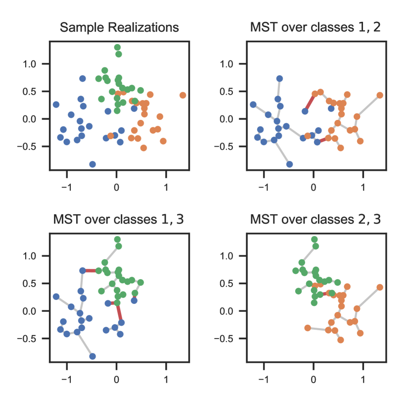
    ninj:=ninj(𝐗)assignsubscriptsubscript𝑛𝑖subscript𝑛𝑗subscriptsubscript𝑛𝑖subscript𝑛𝑗𝐗\mathfrak{R}_{n_{i}n_{j}}:=\mathfrak{R}_{n_{i}n_{j}}(\mathbf{X}) is the number of dichotomous edges in a Euclidean minimal spanning tree (MST) spanning the samples in the pairwise union of samples with labels i𝑖i and j𝑗j , 𝐗(i)𝐗(j)𝕊(i)𝕊(j)superscript𝐗𝑖superscript𝐗𝑗superscript𝕊𝑖superscript𝕊𝑗\mathbf{X}^{(i)}\cup\mathbf{X}^{(j)}\in\mathbb{S}^{(i)}\cup\mathbb{S}^{(j)}, where 𝐗(k)={(𝐱i,yi)}i=1,Yi=knsuperscript𝐗𝑘superscriptsubscriptsubscript𝐱𝑖subscript𝑦𝑖formulae-sequence𝑖1subscript𝑌𝑖𝑘𝑛\mathbf{X}^{(k)}=\{(\mathbf{x}_{i},y_{i})\}_{i=1,Y_{i}=k}^{n}. A dichotomous edge is an edge that connects a sample from class i𝑖i to a sample from class j𝑗j. The pairwise FR statistic ninjsubscriptsubscript𝑛𝑖subscript𝑛𝑗\mathfrak{R}_{n_{i}n_{j}} for three classes is illustrated in Fig 1.

  • 2.

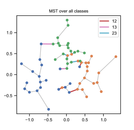
    ni,nj(ij):=ni,nj(ij)(𝐗)assignsubscriptsuperscript𝑖𝑗subscript𝑛𝑖subscript𝑛𝑗subscriptsuperscript𝑖𝑗subscript𝑛𝑖subscript𝑛𝑗𝐗\mathfrak{R}^{(ij)}_{n_{i},n_{j}}:=\mathfrak{R}^{(ij)}_{n_{i},n_{j}}(\mathbf{X}) is the number of dichotomous edges connecting a sample from class i𝑖i to a sample from class j𝑗j in the global MST constructed on all samples with all classes 1,2,m12𝑚1,2\ldots,m i.e. k=1m{(𝐱i,yi)}i=1,yi=knsuperscriptsubscript𝑘1𝑚superscriptsubscriptsubscript𝐱𝑖subscript𝑦𝑖formulae-sequence𝑖1subscript𝑦𝑖𝑘𝑛\bigcup\limits_{k=1}^{m}\{(\mathbf{x}_{i},y_{i})\}_{i=1,y_{i}=k}^{n} or 𝐗(1)𝐗(2)𝐗(m)𝕊(1)𝕊(2)𝕊(m)superscript𝐗1superscript𝐗2superscript𝐗𝑚superscript𝕊1superscript𝕊2superscript𝕊𝑚\mathbf{X}^{(1)}\cup\mathbf{X}^{(2)}\cup\dots\cup\mathbf{X}^{(m)}\in\mathbb{S}^{(1)}\cup\mathbb{S}^{(2)}\cup\dots\mathbb{S}^{(m)} where 𝐗(k)={(𝐱i,yi)}i=1,yi=knsuperscript𝐗𝑘superscriptsubscriptsubscript𝐱𝑖subscript𝑦𝑖formulae-sequence𝑖1subscript𝑦𝑖𝑘𝑛\mathbf{X}^{(k)}=\{(\mathbf{x}_{i},y_{i})\}_{i=1,y_{i}=k}^{n}, k=1,,m𝑘1𝑚k=1,\ldots,m. Fig 2 represents the generalized FR statistic for three classes.

Using the theory in [10] and [9], the estimator ni,njsubscriptsubscript𝑛𝑖subscript𝑛𝑗\mathfrak{R}_{n_{i},n_{j}} is a statistically consistent estimator of the pairwise HP-bound for classifying class i𝑖i vs. class j𝑗j. This yields an estimate of the bounds (11) on multi-class BER, requiring the construction of (m2)binomial𝑚2m\choose 2 MSTs spanning all distinct pairs of label classes. The next theorem implies that ni,nj(ij)subscriptsuperscript𝑖𝑗subscript𝑛𝑖subscript𝑛𝑗\mathfrak{R}^{(ij)}_{n_{i},n_{j}} can be used to estimate the tighter bound on multi-class BER given in Theorem 1 using only a single global MST.
Refer to caption
Figure 1: Estimating ni,njsubscriptsubscript𝑛𝑖subscript𝑛𝑗\mathfrak{R}_{n_{i},n_{j}} for three classes. A set of m(m1)/2𝑚𝑚12m(m-1)/2 Euclidean MSTs are computed for each unordered pair of classes {(i,j)}i>jsubscript𝑖𝑗𝑖𝑗\{(i,j)\}_{i>j}, and then the dichotomous edges (in red) are counted to find ni,njsubscriptsubscript𝑛𝑖subscript𝑛𝑗\mathfrak{R}_{n_{i},n_{j}}.
Refer to caption
Figure 2: Estimating ni,nj(ij)subscriptsuperscript𝑖𝑗subscript𝑛𝑖subscript𝑛𝑗\mathfrak{R}^{(ij)}_{n_{i},n_{j}} for three classes. A single MST is constructed over all classes i=1,2,3𝑖123i=1,2,3 of points. For each (i,j)𝑖𝑗(i,j), count the edges connecting points from classes i𝑖i and j𝑗j. These edges are shown in 3 different colors each corresponding to the three types of pairs (i,j)=(1,2),(2,3),(1,3)𝑖𝑗122313(i,j)=(1,2),(2,3),(1,3).
Theorem 4

Let 𝐗={(𝐱i,yi)}i=1n𝐗superscriptsubscriptsubscript𝐱𝑖subscript𝑦𝑖𝑖1𝑛\mathbf{X}=\{(\mathbf{x}_{i},y_{i})\}_{i=1}^{n} be an i.i.d. m𝑚m-class labeled sample and nk=i=1nI(yi=k)subscript𝑛𝑘superscriptsubscript𝑖1𝑛𝐼subscript𝑦𝑖𝑘n_{k}=\sum_{i=1}^{n}I(y_{i}=k), be the cardinality of samples with label k𝑘k. For distinct classes i,j𝑖𝑗i,j let i,j=1,,mformulae-sequence𝑖𝑗1𝑚i,j=1,\dots,m, ni,njsubscript𝑛𝑖subscript𝑛𝑗n_{i},n_{j}\rightarrow\infty, n𝑛n\rightarrow\infty such that ni/npisubscript𝑛𝑖𝑛subscript𝑝𝑖n_{i}/n\rightarrow p_{i} and nj/npjsubscript𝑛𝑗𝑛subscript𝑝𝑗n_{j}/n\rightarrow p_{j}. Then

ni,nj(ij)(𝐗)2nδijm(a.s.)subscriptsuperscript𝑖𝑗subscript𝑛𝑖subscript𝑛𝑗𝐗2𝑛subscriptsuperscript𝛿𝑚𝑖𝑗(a.s.)\displaystyle\frac{\mathfrak{R}^{(ij)}_{n_{i},n_{j}}(\mathbf{X})}{2n}\displaystyle\longrightarrow\delta^{m}_{ij}\;\;\;\;\hbox{(a.s.)} (20)

The proof of Theorem 4 is given in Appendix G.

V Simulation Study

Here we illustrate the proposed method for learning bounds on Bayes error rate (BER). Section V-A focuses on numerical comparison of the upper bounds in (8), (12), (14) and lower bounds in (8), (13), (15). Section V-B focuses on the empirical estimation of these bounds, including a comparison of runtime.
Refer to caption
Refer to caption
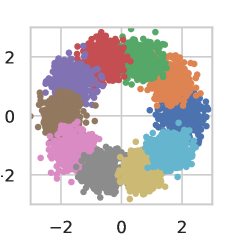
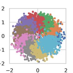
Figure 3: Example of generated data for experiments. The data on the left has 10 classes whose means are arranged around a circle with mean parameter μ=1𝜇1\mu=1. The data on the right has 10 classes, with mean parameter μ=2𝜇2\mu=2. In both cases, σ2=0.1superscript𝜎20.1\sigma^{2}=0.1, and both plots show a sample of 5000 data points.
Refer to caption
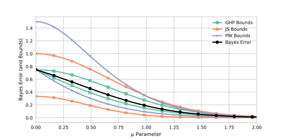
Figure 4: Bounds on the Bayes error for m=4𝑚4m=4 and uniform priors. We note that even for a relatively small number of classes, the proposed new GHP upper and lower bound are much tighter than the competitors. For this experiment, σ2=0.3superscript𝜎20.3\sigma^{2}=0.3.

For each of the following simulations, data is generated in the following way: given m𝑚m classes with priors p1,p2,,pmsubscript𝑝1subscript𝑝2subscript𝑝𝑚p_{1},p_{2},\ldots,p_{m}, the class conditional distributions are mean shifted bivariate normal: fi𝒩(μi,σ2I)similar-tosubscript𝑓𝑖𝒩subscript𝜇𝑖superscript𝜎2𝐼f_{i}\sim\mathcal{N}(\mu_{i},\sigma^{2}I). The means μisubscript𝜇𝑖\mu_{i} are arranged uniformly around the circumference of a circle of radius μ𝜇\mu:

μi=[μcos(2πim),μsin(2πim)].subscript𝜇𝑖𝜇2𝜋𝑖𝑚𝜇2𝜋𝑖𝑚\mu_{i}=\left[\mu\cos\left(2\pi\frac{i}{m}\right),\mu\sin\left(2\pi\frac{i}{m}\right)\right].

Fig. 3 shows two examples for 5000 points and 10 classes and σ2=0.1superscript𝜎20.1\sigma^{2}=0.1, with the left plot having mean parameter μ=0.7𝜇0.7\mu=0.7, and the right plot setting μ=2𝜇2\mu=2. Unless stated otherwise, the feature dimension is d=2𝑑2d=2.

Note that throughout this section, we compute Bayes error rate using Monte Carlo method. Specifically, we rewrite ϵmsuperscriptitalic-ϵ𝑚\epsilon^{m} in terms of expectation 𝔼𝐗subscript𝔼𝐗\mathbb{E}_{\mathbf{X}} i.e.

ϵm=𝔼𝐗[1maxi=1,,mp(i|𝐱)],superscriptitalic-ϵ𝑚subscript𝔼𝐗delimited-[]1subscript𝑖1𝑚𝑝conditional𝑖𝐱\displaystyle\epsilon^{m}=\displaystyle\mathbb{E}_{\mathbf{X}}\Big{[}1-\max\limits_{i=1,\dots,m}p(i|\mathbf{x})\Big{]}, (21)

In addition, we know that p(i|𝐱)=fi(𝐱)pi/fm(𝐱)𝑝conditional𝑖𝐱subscript𝑓𝑖𝐱subscript𝑝𝑖superscript𝑓𝑚𝐱p(i|\mathbf{x})=f_{i}(\mathbf{x})p_{i}/f^{m}(\mathbf{x}) and fi𝒩(μi,σ2I)similar-tosubscript𝑓𝑖𝒩subscript𝜇𝑖superscript𝜎2𝐼f_{i}\sim\mathcal{N}(\mu_{i},\sigma^{2}I). Therefore we generate sample from fmsuperscript𝑓𝑚f^{m} distribution and compute the RHS in (21) for the generated points, then we take the average to compute true BER.

V-A Comparison of bounds

We first explore how the difficulty of the classification problem affects the bounds. Fig. 4 shows upper and lower bounds of the Bayes error rate for each type of bound as a function of the mean parameter μ𝜇\mu. Here, the number of classes m𝑚m is 4. Note that when μ𝜇\mu is smaller and the classes are poorly separated (creating a harder classification problem), both the Jensen-Shannon (JS) and pairwise (PW) upper bounds perform poorly and become trivial, exceeding one. However, for relatively small m𝑚m, the pairwise lower bound remains fairly tight. The proposed GHP bounds are uniformly better than either the JS or PW bounds, as predicted by the theory. Further, note that the proposed bound is tight around the actual Bayes error rate (BER). Finally, as μ𝜇\mu grows and the classes become well separated, the JS and PW bounds become tighter to the Bayes error. In light of Theorem 1, this makes sense for the pairwise bounds, as well separated classes cause the pairwise Henze-Penrose divergence and the GHP integral to become equivalent.

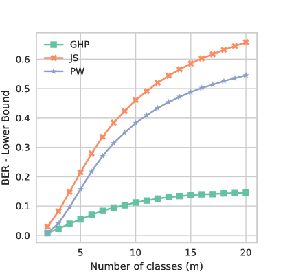
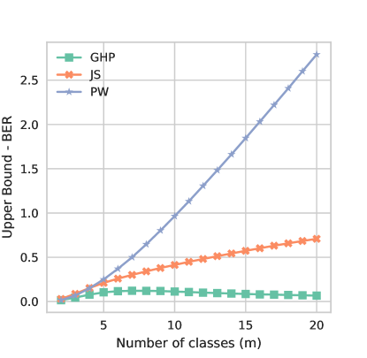
The difference between the bounds and the BER, called the tightness of the bound as a function of m𝑚m is shown in Fig. 5 and Fig. 6 for upper bounds and lower bounds, respectively. Fig. 5 highlights our proposed GHP bound’s ability to stay close to the BER, even as the class size continues to increase. In comparison, both the JS and pairwise upper bounds continue to drift farther away from the Bayes error. Fig. 6 shows a similar effectiveness in the proposed lower bound, although both the JS and pairwise bounds have better behavior than in Fig. 5, due to the lower bounds being guaranteed to be greater than or equal to 0.
Refer to caption
Figure 5: Tightness of upper bound vs. m𝑚m, where tightness is quantified as the difference between the upper bound and the true BER. This experiment was performed for μ=1𝜇1\mu=1. The pairwise upper bound quickly becomes useless as m𝑚m increases. The JS bound performs slightly better, but only our proposed GHP upper bound stays close to the Bayes error.
Refer to caption
Figure 6: Tightness of lower bound vs. m𝑚m, defined as the difference between the BER and the lower bound. This experiment was performed for μ=1𝜇1\mu=1. In the proposed GHP bound, there is a slight decrease in tightness as m𝑚m increases. However, it is much smaller in comparison with the pairwise and JS bound.

V-B Statistical consistency and runtime

This section illustrates the improvement in both statistical accuracy and runtime performance of the proposed generalized HP (GHP) approach as compared to the JS and pairwise HP (PW) methods of [2] and [1].

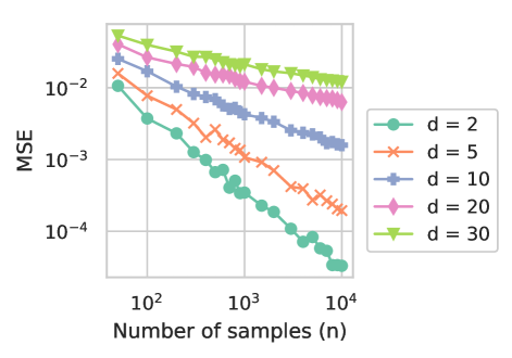
Fig. 7 Shows the MSE between the estimated and true upper bound as a function of the number of samples n𝑛n, for different feature dimensions d𝑑d. The behavior of the lower bound convergence has analogous behavior and is not shown. Note that as d𝑑d increases, the MSE grows, illustrating the well known curse of dimensionality for high dimensional datasets.
Refer to caption
Figure 7: Convergence in MSE of MST estimate of the proposed GHP upper bound to the true upper bound on BER. The simulation parameters were as in Fig. 3 for μ=0.7𝜇0.7\mu=0.7 and σ2=0.1superscript𝜎20.1\sigma^{2}=0.1, and the results were averaged over 100 trials. For d>2𝑑2d>2, d2𝑑2d-2 dimensions had zero mean with Gaussian noise having variance 0.1.

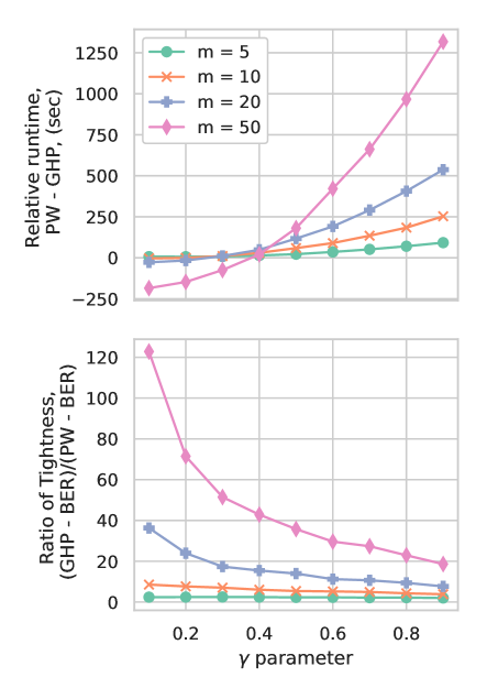
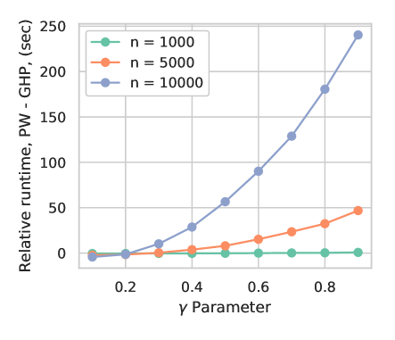
Figs. 8 and 9 show the relative runtime of the proposed method in comparison with the pairwise HP method. For each of these figures, we introduce a parameter γ𝛾\gamma, which controls the prior class imbalance in the problem. For a particular γ𝛾\gamma and number of classes m𝑚m, we create priors p1=γ,p2=p3==pm=(1γ)/(m1)formulae-sequencesubscript𝑝1𝛾subscript𝑝2subscript𝑝3subscript𝑝𝑚1𝛾𝑚1p_{1}=\gamma,p_{2}=p_{3}=\ldots=p_{m}=(1-\gamma)/(m-1). For γ=1/m𝛾1𝑚\gamma=1/m, all class probabilities are the same; there is no imbalance. A larger class imbalance will cause the pairwise estimation procedure to perform many large MST calculations, which significantly increases the runtime of the algorithm. Fig. 8 shows the relative runtime (pairwise - proposed method) as a function of γ𝛾\gamma, for different m𝑚m, along with the ratio of tightness of GHP compared with PW for the upper bound of the BER. Here, we set n=10000,μ=1,σ2=0.3.formulae-sequence𝑛10000formulae-sequence𝜇1superscript𝜎20.3n=10000,\mu=1,\sigma^{2}=0.3. Observe that for large number of classes and small class imbalance γ𝛾\gamma, the pairwise method is slightly faster but, in this regime PW yields a useless bound that is overly loose - the proposed GHP bound is over 120 times tighter than the pairwise bound in this case. As γ𝛾\gamma grows, we see significant relative speedup of the proposed GHP method relative to the other methods. From Fig. 11 it is evident that, while the PW bound has faster computation time in the regime of small γ𝛾\gamma (graph in bottom panel), it is very loose in this small γ𝛾\gamma regime (graph in top panel).

Refer to caption
Figure 8: Relative runtime of pairwise and proposed GHP algorithm vs. class imbalance parameter γ𝛾\gamma, and ratio of tightness of GHP compared with PW, where tightness is defined by the upper bound minus the BER. For large class imbalance (large γ𝛾\gamma), and large m𝑚m, the proposed GHP method achieves significant speedup, while for small class imbalance, the PW bound becomes overly loose.

Fig 9 shows the relative runtime as a function of γ𝛾\gamma, for different sample sizes n𝑛n, with m=10,μ=1,formulae-sequence𝑚10𝜇1m=10,\mu=1, and σ2=0.3superscript𝜎20.3\sigma^{2}=0.3. Similarly to Fig. 8, the greatest speedup occurs when n𝑛n and γ𝛾\gamma are large.

Refer to caption
Figure 9: Relative runtime of pairwise and proposed GHP algorithm vs. class imbalance parameter γ𝛾\gamma. For large γ𝛾\gamma, and large sample size n𝑛n, the proposed method achieves significant speedup.

VI Real Data Experiments

VI-A Using Bounds as Feature Extraction Quality

We utilize our proposed bounds to explore feature generation for the MNIST dataset. The MNIST dataset consists of grey-scale thumbnails, 28 x 28 pixels, of hand-written digits 0 - 9. It consists of a training set of 60,000 examples, and a test set of 10,000 examples. The digits have been size-normalized and centered in a fixed-size image. MNIST has been well studied in the literature, and is known to have a low error-rate. To illustrate the utility of the proposed BER bound learning approach, we estimate the Bayes error rate bounds as a function of feature dimension. Specifically, we focus on PCA and a simple autoencoder. The validity of the proposed lower bound is demonstrated by comparison to the accuracy of three types of classifiers: the K-NN classifier, linear SVM, and a random forest classifier.

Table I: Bounds on the Bayes Error and Classifier Test Error Rates for different feature sets.
Bayes Error Bounds and Error Rates for MNIST Feature Sets
Features lower bound upper bound Linear SVM K-NN, K=3 Rand. For.
PCA-4 0.247 0.427 0.449 0.392 0.370
PCA-8 0.070 0.135 0.241 0.107 0.129
PCA-16 0.029 0.058 0.166 0.037 0.077
PCA-32 0.020 0.040 0.113 0.026 0.073
Autoencoder-4 0.290 0.486 0.662 0.442 0.412
Autoencoder-8 0.097 0.184 0.317 0.144 0.155
Autoencoder-16 0.041 0.082 0.213 0.058 0.099
Autoencoder-32 0.026 0.052 0.144 0.032 0.086

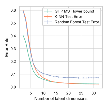
The PCA results are shown in Fig. 10. Plotted are the estimated lower bound for the BER and the test error rates of the 3-NN and Random Forest classifier versus the number of principal components used. As expected, the test errors of both classifiers are greater than the lower bound for Bayes error. Further, it is evident that no more than 20 latent dimensions are needed in order to minimize the lower bound, which is confirmed by the behavior of the test errors of the classifiers implemented.
Refer to caption
Figure 10: Number of latent dimension for PCA vs. error rates and estimated lower bound. The k-NN classifier test error (orange curve) approaching the proposed lower bound (green curve) as the number of latent dimensions increases beyond 15, establishing that the k-NN comes close to achieving optimal performance.

Table I shows Bayes error bounds and error rates for the MNIST feature sets. Autoencoder-X or PCA-X are feature sets that use X latent dimensions or X principal components, respectively. The autoencoder is a 1-layer autoencoder, and trained using Adagrad. Interestingly, we see that PCA-32 feature set outperforms autoencoder-32. More layers or a convolutional model could assist the autoencoder in achieving lower bounds and test error rates.

VI-B Application to CNN Network

Another application of the proposed GHP bounds is to explore the layer-by-layer behavior of neural networks. The cumulative effects on classification performance of the layers can be analyzed by evaluating the proposed bounds at each intermediate layer output. In order to compare similar numbers of features, auxiliary layers — in this case a ReLu and Softmax layer — are added after each intermediate layer that mimic the final two layers in the network. Figure 11 shows a graphical depiction of the architecture. We utilize convolutional and max pooling layers, and test image datasets using this framework.

Refer to caption
Figure 11: Convolutional neural network architecture. We utilize 3 convolutional and max-pooling layers, along with two dense layers at the end, as well as in the auxiliary layers. The auxiliary layers are used to be able to compare the evolution of layer-by-layer classification bounds for different CNN architectures using our proposed multiclass Bayes error estimator. Each convolutional layer has 16 channels.

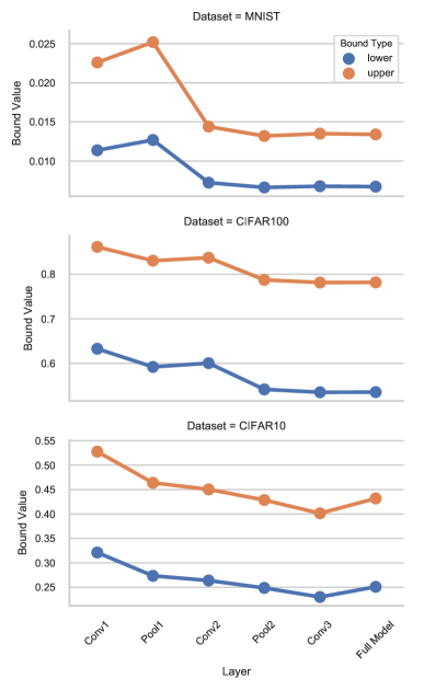
The training proceeds as follows. The main pipeline is trained, and then these layers are frozen. Using these frozen layers, the auxiliary layers are then trained. Each part of the training used AdaGrad. Finally, feature output is taken at each endpoint for the auxiliary layers, and the bounds are subsequently calculated. Each layer was initialized using standard random Normal variables, and the training was done for 25 runs of the total dataset in question. Three datasets are utilized in this fashion: MNIST, CIFAR10, and CIFAR100. The results are shown in Figure 12.
Refer to caption
Figure 12: Performance bounds on the neural network, layer by layer. Most additional convolutional layer improves the performance of the overall network. Further, max-pooling does not significantly reduce the performance, as expected.

We note that, as expected, additional convolutional layers improves the performance of the overall neural net. Further, we see that max-pooling does not significantly affect the performance overall as measured by the proposed bounds, even though it is a downsampling operation. We further see that the bounds are able to distinguish between easy classification datasets such as MNIST, and more challenging problems such as CIFAR100.

VII Conclusion

In this paper, a new bound on the Bayes error rate of multiclass classification was introduced. It was established by theory and simulation that the proposed bound is tighter than both the pairwise Henze-Penrose bound and the generalized Jenson-Shannon bound. Furthermore, a fast and efficient empirical estimator was presented that allows one to learn the bound from training data without the need for density estimation. The estimation method is based on the global minimal spanning tree that spans all labeled features over feature space, allowing for a more computationally tractable approach than the standard practice of summing estimates of pairwise BERs. The statistical complexity and statistical rates of convergence of the multiclass estimator would be useful for predicting the number of samples required to attain a specified accuracy of estimation of the proposed multiclass Bayes error bound. This is important area for future work. The proposed bound learning method was illustrated on the MNIST dataset.

Appendix A Proofs of Main Theorems

Here we first provide further discussion on (6) and (7) and then prove Theorems 1-4. Throughout this section, we use notations δijsubscript𝛿𝑖𝑗\delta_{ij} and δijmsuperscriptsubscript𝛿𝑖𝑗𝑚\delta_{ij}^{m} for FR and generalized FR test statistic, as defined in the paper. D𝐷D represents the HP divergence and f(m)(𝐱)superscript𝑓𝑚𝐱f^{(m)}(\mathbf{x}) is the marginal distribution of random vector 𝐗𝐗\mathbf{X}; 𝔼𝔼\mathbb{E} stands for expectation.

A-A Discussion on (6) and (7)

The relation (6) can be easily derived. Here we provide the proof of relation (7). It can be seen that there exists a constant C1subscript𝐶1C_{1} depending on the pisubscript𝑝𝑖p_{i} and pjsubscript𝑝𝑗p_{j} such that for every fisubscript𝑓𝑖f_{i} and fjsubscript𝑓𝑗f_{j}

fi(𝐱)fj(𝐱)C1(pifi(𝐱)+pjfj(𝐱))2.subscript𝑓𝑖𝐱subscript𝑓𝑗𝐱subscript𝐶1superscriptsubscript𝑝𝑖subscript𝑓𝑖𝐱subscript𝑝𝑗subscript𝑓𝑗𝐱2f_{i}(\mathbf{x})f_{j}(\mathbf{x})\leq C_{1}\left(p_{i}f_{i}(\mathbf{x})+p_{j}f_{j}(\mathbf{x})\right)^{2}. (22)

Set

gij(𝐱):=(pifi(𝐱)+pjfj(𝐱))ki,jpkfk(𝐱)/f(m)(𝐱).assignsubscript𝑔𝑖𝑗𝐱subscript𝑝𝑖subscript𝑓𝑖𝐱subscript𝑝𝑗subscript𝑓𝑗𝐱subscript𝑘𝑖𝑗subscript𝑝𝑘subscript𝑓𝑘𝐱superscript𝑓𝑚𝐱g_{ij}(\mathbf{x}):=\displaystyle\left(p_{i}f_{i}(\mathbf{x})+p_{j}f_{j}(\mathbf{x})\right)\displaystyle\sum\limits_{k\neq i,j}p_{k}f_{k}(\mathbf{x})\big{/}f^{(m)}(\mathbf{x}). (23)

The inequality (22) is equivalent to

0fi(𝐱)fj(𝐱)(1pifi(𝐱)+pjfj(𝐱)1f(m)(𝐱))C1gij(𝐱).0subscript𝑓𝑖𝐱subscript𝑓𝑗𝐱1subscript𝑝𝑖subscript𝑓𝑖𝐱subscript𝑝𝑗subscript𝑓𝑗𝐱1superscript𝑓𝑚𝐱subscript𝐶1subscript𝑔𝑖𝑗𝐱0\leq f_{i}(\mathbf{x})f_{j}(\mathbf{x})\left(\displaystyle\frac{1}{p_{i}f_{i}(\mathbf{x})+p_{j}f_{j}(\mathbf{x})}-\frac{1}{f^{(m)}(\mathbf{x})}\right)\leq C_{1}\;g_{ij}(\mathbf{x}). (24)

Therefore

fi(𝐱)fj(𝐱)pifi(𝐱)+pjfj(𝐱)d𝐱fi(𝐱)fj(𝐱)f(m)(𝐱)d𝐱+C1(g𝑖𝑗(𝐱)d𝐱)subscript𝑓𝑖𝐱subscript𝑓𝑗𝐱subscript𝑝𝑖subscript𝑓𝑖𝐱subscript𝑝𝑗subscript𝑓𝑗𝐱differential-d𝐱subscript𝑓𝑖𝐱subscript𝑓𝑗𝐱superscript𝑓𝑚𝐱differential-d𝐱subscript𝐶1subscript𝑔𝑖𝑗𝐱differential-d𝐱\begin{array}[]{l}\displaystyle\int\displaystyle\frac{f_{i}(\mathbf{x})f_{j}(\mathbf{x})}{p_{i}f_{i}(\mathbf{x})+p_{j}f_{j}(\mathbf{x})}\rm{d}\mathbf{x}\leq{\it\displaystyle\int{\it\displaystyle\frac{f_{i}(\mathbf{x})f_{j}(\mathbf{x})}{f^{(m)}(\mathbf{x})}\rm{d}\mathbf{x}}+C_{1}\Big{(}\displaystyle\int g_{ij}(\mathbf{x})\;\rm{d}\mathbf{x}\Big{)}}\end{array} (25)

On the other hand, we have

D(p~ijfi+p~jifj,ki,jp~kijfk)=11(pi+pj)ri,jprgij(𝐱)d𝐱,𝐷subscript~𝑝𝑖𝑗subscript𝑓𝑖subscript~𝑝𝑗𝑖subscript𝑓𝑗subscript𝑘𝑖𝑗superscriptsubscript~𝑝𝑘𝑖𝑗subscript𝑓𝑘absent11subscript𝑝𝑖subscript𝑝𝑗subscript𝑟𝑖𝑗subscript𝑝𝑟subscript𝑔𝑖𝑗𝐱differential-d𝐱\begin{array}[]{l}D\Big{(}\widetilde{p}_{ij}f_{i}+\widetilde{p}_{ji}f_{j},\displaystyle\sum\limits_{k\neq i,j}\widetilde{p}_{k}^{ij}f_{k}\Big{)}=\\ \qquad\qquad 1-\displaystyle\frac{1}{(p_{i}+p_{j})\displaystyle\sum\limits_{r\neq i,j}p_{r}}\displaystyle\int g_{ij}(\mathbf{x})\;\rm{d}\mathbf{x},\end{array} (26)

where p~ijsubscript~𝑝𝑖𝑗\widetilde{p}_{ij} and p~jisubscript~𝑝𝑗𝑖\widetilde{p}_{ji} are as before and p~kij=pk/ri,jprsuperscriptsubscript~𝑝𝑘𝑖𝑗subscript𝑝𝑘subscript𝑟𝑖𝑗subscript𝑝𝑟\widetilde{p}_{k}^{ij}=p_{k}\big{/}\displaystyle\sum\limits_{r\neq i,j}p_{r}. Hence,

gij(𝐱)d𝐱=C2{1D(p~𝑖𝑗fi+p~𝑗𝑖fj,ki,jp~k𝑖𝑗fk)}.subscript𝑔𝑖𝑗𝐱differential-d𝐱subscriptC21𝐷subscript~𝑝𝑖𝑗subscript𝑓𝑖subscript~𝑝𝑗𝑖subscript𝑓𝑗subscript𝑘𝑖𝑗superscriptsubscript~𝑝𝑘𝑖𝑗subscript𝑓𝑘\int g_{ij}(\mathbf{x})\;\rm{d}\mathbf{x}=C_{2}{\it\Big{\{}1-D\Big{(}\widetilde{p}_{ij}f_{i}+\widetilde{p}_{ji}f_{j},\displaystyle\sum\limits_{k\neq i,j}\widetilde{p}_{k}^{ij}f_{k}\Big{)}\Big{\}}}. (27)

where C2subscript𝐶2C_{2} is a constant depending on priors p1,p2,pmsubscript𝑝1subscript𝑝2subscript𝑝𝑚p_{1},p_{2},\dots p_{m}. This together with (25) implies that there exists a constant C𝐶C depending only on priors p1,p2,,pmsubscript𝑝1subscript𝑝2subscript𝑝𝑚p_{1},p_{2},\dots,p_{m} such that

fi(𝐱)fj(𝐱)pifi(𝐱)+pjfj(𝐱)d𝐱fi(𝐱)fj(𝐱)f(m)(𝐱)d𝐱+C(1D(p~ijfi+p~jifj,ki,jp~kijfk)),subscript𝑓𝑖𝐱subscript𝑓𝑗𝐱subscript𝑝𝑖subscript𝑓𝑖𝐱subscript𝑝𝑗subscript𝑓𝑗𝐱differential-d𝐱subscript𝑓𝑖𝐱subscript𝑓𝑗𝐱superscript𝑓𝑚𝐱differential-d𝐱missing-subexpression𝐶1𝐷subscript~𝑝𝑖𝑗subscript𝑓𝑖subscript~𝑝𝑗𝑖subscript𝑓𝑗subscript𝑘𝑖𝑗superscriptsubscript~𝑝𝑘𝑖𝑗subscript𝑓𝑘\begin{array}[]{l}\displaystyle\int\displaystyle\frac{f_{i}(\mathbf{x})f_{j}(\mathbf{x})}{p_{i}f_{i}(\mathbf{x})+p_{j}f_{j}(\mathbf{x})}\rm{d}\mathbf{x}\leq{\it\displaystyle\int\displaystyle\frac{f_{i}(\mathbf{x})f_{j}(\mathbf{x})}{f^{(m)}(\mathbf{x})}\rm{d}\mathbf{x}}\\ \\ \qquad\qquad+C\Big{(}1-D\Big{(}\widetilde{p}_{ij}f_{i}+\widetilde{p}_{ji}f_{j},\displaystyle\sum\limits_{k\neq i,j}\widetilde{p}_{k}^{ij}f_{k}\Big{)}\Big{)},\end{array} (28)

By recalling HPijsubscriptHP𝑖𝑗{\rm HP}_{ij} (4) and GHPijmsubscriptsuperscriptGHP𝑚𝑖𝑗{\rm GHP}^{m}_{ij} (5) we conclude the result.

A-B Theorem 1

To derive the inequality in (14), first we need to prove the following lemma:

Lemma 1

Let a1,a2,,amsubscript𝑎1subscript𝑎2subscript𝑎𝑚a_{1},a_{2},\dots,a_{m} be a probability distribution on m𝑚m classes so that i=1mai=1superscriptsubscript𝑖1𝑚subscript𝑎𝑖1\displaystyle\sum\limits_{i=1}^{m}a_{i}=1. Then

1maxiai2i=1m1j=i+1maiaj.1subscript𝑖subscript𝑎𝑖2superscriptsubscript𝑖1𝑚1superscriptsubscript𝑗𝑖1𝑚subscript𝑎𝑖subscript𝑎𝑗1-\max\limits_{i}a_{i}\leq 2\displaystyle\sum\limits_{i=1}^{m-1}\sum\limits_{j=i+1}^{m}a_{i}a_{j}. (29)
Proof:

Assume, without loss of generality, that the aisubscript𝑎𝑖a_{i} have been reordered in such a way that amsubscript𝑎𝑚a_{m} is the largest. So it is sufficient to prove that

1am2i=1m1j=i+1maiaj.1subscript𝑎𝑚2superscriptsubscript𝑖1𝑚1superscriptsubscript𝑗𝑖1𝑚subscript𝑎𝑖subscript𝑎𝑗1-a_{m}\leq 2\displaystyle\sum\limits_{i=1}^{m-1}\sum\limits_{j=i+1}^{m}a_{i}a_{j}. (30)

Since i=1mai=1superscriptsubscript𝑖1𝑚subscript𝑎𝑖1\displaystyle\sum\limits_{i=1}^{m}a_{i}=1 then

1am=i=1m1ai=i=1m1j=1maiaj.1subscript𝑎𝑚superscriptsubscript𝑖1𝑚1subscript𝑎𝑖superscriptsubscript𝑖1𝑚1superscriptsubscript𝑗1𝑚subscript𝑎𝑖subscript𝑎𝑗1-a_{m}=\displaystyle\sum\limits_{i=1}^{m-1}a_{i}=\displaystyle\sum\limits_{i=1}^{m-1}\sum\limits_{j=1}^{m}a_{i}a_{j}.

Therefore we need to show that

i=1m1j=1maiaj2i=1m1j=i+1maiaj.superscriptsubscript𝑖1𝑚1superscriptsubscript𝑗1𝑚subscript𝑎𝑖subscript𝑎𝑗2superscriptsubscript𝑖1𝑚1superscriptsubscript𝑗𝑖1𝑚subscript𝑎𝑖subscript𝑎𝑗\displaystyle\sum\limits_{i=1}^{m-1}\sum\limits_{j=1}^{m}a_{i}a_{j}\leq 2\displaystyle\sum\limits_{i=1}^{m-1}\sum\limits_{j=i+1}^{m}a_{i}a_{j}. (31)

The LHS in (31) is

i=1m1j=1maiaj=2i=1m2j=i+1m1aiaj+i=1m1aiam+i=1m1ai2.superscriptsubscript𝑖1𝑚1superscriptsubscript𝑗1𝑚subscript𝑎𝑖subscript𝑎𝑗2superscriptsubscript𝑖1𝑚2superscriptsubscript𝑗𝑖1𝑚1subscript𝑎𝑖subscript𝑎𝑗superscriptsubscript𝑖1𝑚1subscript𝑎𝑖subscript𝑎𝑚superscriptsubscript𝑖1𝑚1superscriptsubscript𝑎𝑖2\displaystyle\sum\limits_{i=1}^{m-1}\sum\limits_{j=1}^{m}a_{i}a_{j}=2\displaystyle\sum\limits_{i=1}^{m-2}\sum\limits_{j=i+1}^{m-1}a_{i}a_{j}+\sum\limits_{i=1}^{m-1}a_{i}a_{m}+\sum\limits_{i=1}^{m-1}a_{i}^{2}. (32)

And the RHS in (31) is written as

2i=1m1j=i+1maiaj=2i=1m2j=i+1m1aiaj+2i=1m1aiam.2superscriptsubscript𝑖1𝑚1superscriptsubscript𝑗𝑖1𝑚subscript𝑎𝑖subscript𝑎𝑗2superscriptsubscript𝑖1𝑚2superscriptsubscript𝑗𝑖1𝑚1subscript𝑎𝑖subscript𝑎𝑗2superscriptsubscript𝑖1𝑚1subscript𝑎𝑖subscript𝑎𝑚2\displaystyle\sum\limits_{i=1}^{m-1}\sum\limits_{j=i+1}^{m}a_{i}a_{j}=2\displaystyle\sum\limits_{i=1}^{m-2}\sum\limits_{j=i+1}^{m-1}a_{i}a_{j}+2\displaystyle\sum\limits_{i=1}^{m-1}a_{i}a_{m}. (33)

Recalling our assumption that amsubscript𝑎𝑚a_{m} is the largest we have

i=1m1ai2i=1m1aiam.superscriptsubscript𝑖1𝑚1superscriptsubscript𝑎𝑖2superscriptsubscript𝑖1𝑚1subscript𝑎𝑖subscript𝑎𝑚\displaystyle\sum\limits_{i=1}^{m-1}a_{i}^{2}\leq\displaystyle\sum\limits_{i=1}^{m-1}a_{i}a_{m}. (34)

This implies that (32)(33)3233(\ref{eq2:lemma1})\leq(\ref{eq3:lemma1}). This concludes (31) and proves our Lemma. ∎

Going back to prove upper bound (14) in Theorem 1, let p1f1(𝐱),p2f2(𝐱),,pmfm(𝐱)subscript𝑝1subscript𝑓1𝐱subscript𝑝2subscript𝑓2𝐱subscript𝑝𝑚subscript𝑓𝑚𝐱p_{1}f_{1}(\mathbf{x}),p_{2}f_{2}(\mathbf{x}),\dots,p_{m}f_{m}(\mathbf{x}) be joint probabilities of 𝐱𝐱\mathbf{x} and i𝑖i. And denote p(i|𝐱):=P(y=i|𝐱)assign𝑝conditional𝑖𝐱𝑃𝑦conditional𝑖𝐱p(i|\mathbf{x}):=P(y=i|\mathbf{x}) where variable y{1,2,,m}𝑦12𝑚y\in\{1,2,\dots,m\} is class label with priors pisubscript𝑝𝑖p_{i}. The BER for m𝑚m classes is given by

ϵm=1max{p1f1(𝐱),,pmfm(𝐱)}d𝐱=𝔼𝐗[1maxi=1,,mp(i|𝐱)],superscriptitalic-ϵ𝑚1subscript𝑝1subscript𝑓1𝐱subscript𝑝𝑚subscript𝑓𝑚𝐱differential-d𝐱missing-subexpressionabsentsubscript𝔼𝐗delimited-[]1subscript𝑖1𝑚𝑝conditional𝑖𝐱missing-subexpression\begin{array}[]{cl}\epsilon^{m}=1-\displaystyle\int\max\big{\{}p_{1}f_{1}(\mathbf{x}),\dots,p_{m}f_{m}(\mathbf{x})\big{\}}\rm{d}\mathbf{x}\\ =\mathbb{E}_{\mathbf{X}}\Big{[}1-\max\limits_{i=1,\dots,m}p(i|\mathbf{x})\Big{]},\end{array} (35)

Moreover the marginal density for random vector 𝐗𝐗\mathbf{X} is

f𝐗(𝐱)=i=1mpifi(𝐱)=f(m)(𝐱),subscript𝑓𝐗𝐱superscriptsubscript𝑖1𝑚subscript𝑝𝑖subscript𝑓𝑖𝐱superscript𝑓𝑚𝐱f_{\mathbf{X}}(\mathbf{x})=\displaystyle\sum\limits_{i=1}^{m}p_{i}f_{i}(\mathbf{x})=f^{(m)}(\mathbf{x}),

And

pipjfi(𝐱)fj(𝐱)f(m)(𝐱)d𝐱=(pifi(𝐱)fm(𝐱))(pjfj(𝐱)f(m)(𝐱))f(m)(𝐱)d𝐱=p(i|𝐱)p(j|𝐱)f(m)(𝐱)d𝐱=𝔼𝐗[p(i|𝐗)p(j|𝐗)].subscript𝑝𝑖subscript𝑝𝑗subscript𝑓𝑖𝐱subscript𝑓𝑗𝐱superscript𝑓𝑚𝐱differential-d𝐱subscript𝑝𝑖subscript𝑓𝑖𝐱superscript𝑓𝑚𝐱subscript𝑝𝑗subscript𝑓𝑗𝐱superscript𝑓𝑚𝐱superscript𝑓𝑚𝐱differential-d𝐱missing-subexpressionabsent𝑝conditional𝑖𝐱𝑝conditional𝑗𝐱superscript𝑓𝑚𝐱differential-d𝐱subscript𝔼𝐗delimited-[]𝑝conditional𝑖𝐗𝑝conditional𝑗𝐗\begin{array}[]{l}\displaystyle{\int}\frac{p_{i}p_{j}f_{i}(\mathbf{x})f_{j}(\mathbf{x})}{f^{(m)}(\mathbf{x})}{\rm d}\mathbf{x}=\displaystyle{\int}\left(\frac{p_{i}f_{i}(\mathbf{x})}{f^{m}(\mathbf{x})}\right)\left(\frac{p_{j}f_{j}(\mathbf{x})}{f^{(m)}(\mathbf{x})}\right)f^{(m)}(\mathbf{x})\rm{d}\mathbf{x}\\ \\ \qquad\quad=\displaystyle{\int}p(i|\mathbf{x})p(j|\mathbf{x})f^{(m)}(\mathbf{x}){\rm d}\mathbf{x}=\mathbb{E}_{\mathbf{X}}\left[p(i|\mathbf{X})p(j|\mathbf{X})\right].\end{array} (36)

Therefore (14) turns into the following claim:

𝔼𝐗[1maxi=1,,mp(i|𝐱)]𝔼𝐗[2i=1m1j=i+1mp(i|𝐗)p(j|𝐗)].subscript𝔼𝐗delimited-[]1subscript𝑖1𝑚𝑝conditional𝑖𝐱subscript𝔼𝐗delimited-[]2superscriptsubscript𝑖1𝑚1superscriptsubscript𝑗𝑖1𝑚𝑝conditional𝑖𝐗𝑝conditional𝑗𝐗\displaystyle\mathbb{E}_{\mathbf{X}}\Big{[}1-\max\limits_{i=1,\dots,m}p(i|\mathbf{x})\Big{]}\leq\mathbb{E}_{\mathbf{X}}\left[2\displaystyle\sum\limits_{i=1}^{m-1}\sum\limits_{j=i+1}^{m}p(i|\mathbf{X})p(j|\mathbf{X})\right]. (37)

We know that i=1mp(i|𝐱)=1superscriptsubscript𝑖1𝑚𝑝conditional𝑖𝐱1\displaystyle\sum\limits_{i=1}^{m}p(i|\mathbf{x})=1. Using Lemma 1 where aisubscript𝑎𝑖a_{i} represents p(i|𝐱)𝑝conditional𝑖𝐱p(i|\mathbf{x}) we have

1maxi=1,,mp(i|𝐱)2i=1m1j=i+1mp(i|𝐗)p(j|𝐗).1subscript𝑖1𝑚𝑝conditional𝑖𝐱2superscriptsubscript𝑖1𝑚1superscriptsubscript𝑗𝑖1𝑚𝑝conditional𝑖𝐗𝑝conditional𝑗𝐗\displaystyle 1-\max\limits_{i=1,\dots,m}p(i|\mathbf{x})\leq 2\displaystyle\sum\limits_{i=1}^{m-1}\sum\limits_{j=i+1}^{m}p(i|\mathbf{X})p(j|\mathbf{X}). (38)

Hence, we prove the inequality (37) and consequently our claim (14).

Next we prove the lower bound (15). The following lemma is required:

Lemma 2

For all a1,a2,,amsubscript𝑎1subscript𝑎2subscript𝑎𝑚a_{1},a_{2},...,a_{m} such that i=1mai=1superscriptsubscript𝑖1𝑚subscript𝑎𝑖1\displaystyle\sum_{i=1}^{m}a_{i}=1, we have the following:

m1m[1(12mm1i=1m1j=i+1maiaj)1/2]1maxiai.𝑚1𝑚delimited-[]1superscript12𝑚𝑚1superscriptsubscript𝑖1𝑚1superscriptsubscript𝑗𝑖1𝑚subscript𝑎𝑖subscript𝑎𝑗121subscript𝑖subscript𝑎𝑖\frac{m-1}{m}\left[1-\left(1-2\frac{m}{m-1}\sum_{i=1}^{m-1}\sum_{j=i+1}^{m}a_{i}a_{j}\right)^{1/2}\right]\leq 1-\max_{i}a_{i}. (39)
Proof:

After some algebra, we rewrite the inequality in the following form:

m(maxiai)22maxiaim2(m1)b,𝑚superscriptsubscript𝑖subscript𝑎𝑖22subscript𝑖subscript𝑎𝑖𝑚2𝑚1𝑏m(\max_{i}a_{i})^{2}-2\max_{i}a_{i}\leq m-2-(m-1)b,

where b=2i=1m1j=i+1maiaj.𝑏2superscriptsubscript𝑖1𝑚1superscriptsubscript𝑗𝑖1𝑚subscript𝑎𝑖subscript𝑎𝑗b=\displaystyle 2\sum_{i=1}^{m-1}\sum_{j=i+1}^{m}a_{i}a_{j}. Without loss of generality, we can assume that the aisubscript𝑎𝑖a_{i}s are ordered, so that amsubscript𝑎𝑚a_{m} is the largest. Then we have that maxiai=1i=1m1ai.subscript𝑖subscript𝑎𝑖1superscriptsubscript𝑖1𝑚1subscript𝑎𝑖\max_{i}a_{i}=1-\displaystyle\sum_{i=1}^{m-1}a_{i}.

Using this equality on the left side, expanding the square, and subtracting m2𝑚2m-2 from both sides, we have:

m(i=1m1ai)2(2m1)i=1m1ai(m1)b.𝑚superscriptsuperscriptsubscript𝑖1𝑚1subscript𝑎𝑖22𝑚1superscriptsubscript𝑖1𝑚1subscript𝑎𝑖𝑚1𝑏m(\sum_{i=1}^{m-1}a_{i})^{2}-(2m-1)\sum_{i=1}^{m-1}a_{i}\leq-(m-1)b. (40)

Expanding terms once again:

i=1m1j=i+1maiaj=i=1m2j=i+1m1aiaj+i=1m1aiam,superscriptsubscript𝑖1𝑚1superscriptsubscript𝑗𝑖1𝑚subscript𝑎𝑖subscript𝑎𝑗superscriptsubscript𝑖1𝑚2superscriptsubscript𝑗𝑖1𝑚1subscript𝑎𝑖subscript𝑎𝑗superscriptsubscript𝑖1𝑚1subscript𝑎𝑖subscript𝑎𝑚\sum_{i=1}^{m-1}\sum_{j=i+1}^{m}a_{i}a_{j}=\sum_{i=1}^{m-2}\sum_{j=i+1}^{m-1}a_{i}a_{j}+\sum_{i=1}^{m-1}a_{i}a_{m}, (41)

and collecting like terms:

mi=1m1ai2+(4m2)i=1m2j=i+1m1aiaj(2m1)i=1m1ai2(m1)i=1m1aiam𝑚superscriptsubscript𝑖1𝑚1superscriptsubscript𝑎𝑖24𝑚2superscriptsubscript𝑖1𝑚2superscriptsubscript𝑗𝑖1𝑚1subscript𝑎𝑖subscript𝑎𝑗2𝑚1superscriptsubscript𝑖1𝑚1subscript𝑎𝑖missing-subexpressionabsent2𝑚1superscriptsubscript𝑖1𝑚1subscript𝑎𝑖subscript𝑎𝑚\begin{array}[]{l}\displaystyle m\sum_{i=1}^{m-1}a_{i}^{2}+(4m-2)\sum_{i=1}^{m-2}\sum_{j=i+1}^{m-1}a_{i}a_{j}-(2m-1)\sum_{i=1}^{m-1}a_{i}\\ \\ \qquad\qquad\leq-\displaystyle 2(m-1)\sum_{i=1}^{m-1}a_{i}a_{m}\end{array} (42)

We note, that since i=1mai=1superscriptsubscript𝑖1𝑚subscript𝑎𝑖1\sum_{i=1}^{m}a_{i}=1, we have the following:

i=1m1ai=i=1m1j=1maiaj=2i=1m2j=i+1m1aiaj+i=1m1aiam+i=1m1ai2.superscriptsubscript𝑖1𝑚1subscript𝑎𝑖superscriptsubscript𝑖1𝑚1superscriptsubscript𝑗1𝑚subscript𝑎𝑖subscript𝑎𝑗2superscriptsubscript𝑖1𝑚2superscriptsubscript𝑗𝑖1𝑚1subscript𝑎𝑖subscript𝑎𝑗superscriptsubscript𝑖1𝑚1subscript𝑎𝑖subscript𝑎𝑚superscriptsubscript𝑖1𝑚1superscriptsubscript𝑎𝑖2\sum_{i=1}^{m-1}a_{i}=\sum_{i=1}^{m-1}\sum_{j=1}^{m}a_{i}a_{j}=2\sum_{i=1}^{m-2}\sum_{j=i+1}^{m-1}a_{i}a_{j}+\sum_{i=1}^{m-1}a_{i}a_{m}+\sum_{i=1}^{m-1}a_{i}^{2}.

Plugging in once more:

(1m)i=1m1ai2(2m1)i=1m1aiam2(m1)i=1m1aiam,1𝑚superscriptsubscript𝑖1𝑚1superscriptsubscript𝑎𝑖22𝑚1superscriptsubscript𝑖1𝑚1subscript𝑎𝑖subscript𝑎𝑚2𝑚1superscriptsubscript𝑖1𝑚1subscript𝑎𝑖subscript𝑎𝑚(1-m)\sum_{i=1}^{m-1}a_{i}^{2}-(2m-1)\sum_{i=1}^{m-1}a_{i}a_{m}\leq-2(m-1)\sum_{i=1}^{m-1}a_{i}a_{m},

or equivalently:

(1m)i=1m1ai2i=1m1aiam0.1𝑚superscriptsubscript𝑖1𝑚1superscriptsubscript𝑎𝑖2superscriptsubscript𝑖1𝑚1subscript𝑎𝑖subscript𝑎𝑚0(1-m)\sum_{i=1}^{m-1}a_{i}^{2}-\sum_{i=1}^{m-1}a_{i}a_{m}\leq 0.

Note that since am=maxiaisubscript𝑎𝑚subscript𝑖subscript𝑎𝑖a_{m}=\max_{i}a_{i}, i=1m1aiami=1m1ai2superscriptsubscript𝑖1𝑚1subscript𝑎𝑖subscript𝑎𝑚superscriptsubscript𝑖1𝑚1superscriptsubscript𝑎𝑖2\displaystyle\sum_{i=1}^{m-1}a_{i}a_{m}\geq\displaystyle\sum_{i=1}^{m-1}a_{i}^{2}, so that

(1m)i=1m1ai2i=1m1aiammi=1m1ai20,1𝑚superscriptsubscript𝑖1𝑚1superscriptsubscript𝑎𝑖2superscriptsubscript𝑖1𝑚1subscript𝑎𝑖subscript𝑎𝑚𝑚superscriptsubscript𝑖1𝑚1superscriptsubscript𝑎𝑖20(1-m)\sum_{i=1}^{m-1}a_{i}^{2}-\sum_{i=1}^{m-1}a_{i}a_{m}\leq-m\sum_{i=1}^{m-1}a_{i}^{2}\leq 0,

since i=1m1ai20superscriptsubscript𝑖1𝑚1superscriptsubscript𝑎𝑖20\displaystyle\sum_{i=1}^{m-1}a_{i}^{2}\geq 0. ∎

Now to prove (15), let p1f1(𝐱),p2f2(𝐱),,pmfm(𝐱)subscript𝑝1subscript𝑓1𝐱subscript𝑝2subscript𝑓2𝐱subscript𝑝𝑚subscript𝑓𝑚𝐱p_{1}f_{1}(\mathbf{x}),p_{2}f_{2}(\mathbf{x}),\dots,p_{m}f_{m}(\mathbf{x}) be joint probabilities of 𝐱𝐱\mathbf{x} and i𝑖i. And denote p(i|𝐱):=P(y=i|𝐱)assign𝑝conditional𝑖𝐱𝑃𝑦conditional𝑖𝐱p(i|\mathbf{x}):=P(y=i|\mathbf{x}) where variable y{1,2,,m}𝑦12𝑚y\in\{1,2,\dots,m\} is class label with priors pisubscript𝑝𝑖p_{i}. By taking the expectation from both sides of (39) when ai=p(i|𝐱)subscript𝑎𝑖𝑝conditional𝑖𝐱a_{i}=p(i|\mathbf{x}), we have

𝔼𝐗[1maxip(i|𝐱)]m1m[1𝔼𝐗(12mm1i=1m1j=i+1mp(i|𝐱)p(j|𝐱))1/2],subscript𝔼𝐗delimited-[]1subscript𝑖𝑝conditional𝑖𝐱absent𝑚1𝑚delimited-[]1subscript𝔼𝐗superscript12𝑚𝑚1superscriptsubscript𝑖1𝑚1superscriptsubscript𝑗𝑖1𝑚𝑝conditional𝑖𝐱𝑝conditional𝑗𝐱12\begin{array}[]{l}\displaystyle\mathbb{E}_{\mathbf{X}}[1-\max_{i}p(i|\mathbf{x})]\\ \quad\geq\displaystyle\frac{m-1}{m}\left[1-\mathbb{E}_{\mathbf{X}}\left(1-2\frac{m}{m-1}\sum_{i=1}^{m-1}\sum_{j=i+1}^{m}p(i|\mathbf{x})p(j|\mathbf{x})\right)^{1/2}\right],\end{array} (43)

Further, since ϕ(𝐱)=𝐱italic-ϕ𝐱𝐱\phi(\mathbf{x})=\sqrt{\mathbf{x}} is a concave function, by applying Jensen inequality the RHS in (43) is lower bounded by

m1m[1(12mm1𝔼𝐗[i=1m1j=i+1mp(i|𝐱)p(j|𝐱)])1/2],𝑚1𝑚delimited-[]1superscript12𝑚𝑚1subscript𝔼𝐗delimited-[]superscriptsubscript𝑖1𝑚1superscriptsubscript𝑗𝑖1𝑚𝑝conditional𝑖𝐱𝑝conditional𝑗𝐱12\displaystyle\frac{m-1}{m}\left[1-\left(1-2\frac{m}{m-1}\mathbb{E}_{\mathbf{X}}\left[\sum_{i=1}^{m-1}\sum_{j=i+1}^{m}p(i|\mathbf{x})p(j|\mathbf{x})\right]\right)^{1/2}\right], (44)

And we know that

𝔼𝐗[p(i|𝐱)p(j|𝐱)]=δijm,subscript𝔼𝐗delimited-[]𝑝conditional𝑖𝐱𝑝conditional𝑗𝐱subscriptsuperscript𝛿𝑚𝑖𝑗\mathbb{E}_{\mathbf{X}}\left[p(i|\mathbf{x})p(j|\mathbf{x})\right]=\delta^{m}_{ij},

and

𝔼𝐗[1maxip(i|𝐱)]=ϵm,subscript𝔼𝐗delimited-[]1subscript𝑖𝑝conditional𝑖𝐱superscriptitalic-ϵ𝑚\mathbb{E}_{\mathbf{X}}[1-\max_{i}p(i|\mathbf{x})]=\epsilon^{m},

then this proves our proposed lower bound in (15).

A-C Theorem 2

To derive (16), the following lemma is required to be proved:

Lemma 3

Let a1,a2,,amsubscript𝑎1subscript𝑎2subscript𝑎𝑚a_{1},a_{2},\dots,a_{m} be probability distributions on m𝑚m classes so i=1mai=1superscriptsubscript𝑖1𝑚subscript𝑎𝑖1\displaystyle\sum\limits_{i=1}^{m}a_{i}=1. Then, for m3𝑚3m\geq 3 and log basis 222, we have

2i=1m1j=i+1maiaj12i=1mailogai.2superscriptsubscript𝑖1𝑚1superscriptsubscript𝑗𝑖1𝑚subscript𝑎𝑖subscript𝑎𝑗12superscriptsubscript𝑖1𝑚subscript𝑎𝑖subscript𝑎𝑖2\displaystyle\sum_{i=1}^{m-1}\sum_{j=i+1}^{m}a_{i}a_{j}\leq-\displaystyle\frac{1}{2}\sum_{i=1}^{m}a_{i}\log a_{i}. (45)
Proof:

The claim in (45) can be rewritten as

4i=1m1j=i+1maiaji=1mailog1ai,4superscriptsubscript𝑖1𝑚1superscriptsubscript𝑗𝑖1𝑚subscript𝑎𝑖subscript𝑎𝑗superscriptsubscript𝑖1𝑚subscript𝑎𝑖1subscript𝑎𝑖4\displaystyle\sum_{i=1}^{m-1}\sum_{j=i+1}^{m}a_{i}a_{j}\leq\displaystyle\sum_{i=1}^{m}a_{i}\log\displaystyle\frac{1}{a_{i}}, (46)

where 0ai10subscript𝑎𝑖10\leq a_{i}\leq 1. In addition we have

4i=1m1j=i+1maiaj=4i=1m2j=i+1m1aiaj+4i=1m1aiam,4superscriptsubscript𝑖1𝑚1superscriptsubscript𝑗𝑖1𝑚subscript𝑎𝑖subscript𝑎𝑗4superscriptsubscript𝑖1𝑚2superscriptsubscript𝑗𝑖1𝑚1subscript𝑎𝑖subscript𝑎𝑗4superscriptsubscript𝑖1𝑚1subscript𝑎𝑖subscript𝑎𝑚4\displaystyle\sum\limits_{i=1}^{m-1}\sum\limits_{j=i+1}^{m}a_{i}a_{j}=4\displaystyle\sum\limits_{i=1}^{m-2}\sum\limits_{j=i+1}^{m-1}a_{i}a_{j}+4\displaystyle\sum\limits_{i=1}^{m-1}a_{i}a_{m}, (47)

and

i=1m1aii=1m1aiami=1m1ai2=2i=1m2j=i+1m1aiaj.superscriptsubscript𝑖1𝑚1subscript𝑎𝑖superscriptsubscript𝑖1𝑚1subscript𝑎𝑖subscript𝑎𝑚superscriptsubscript𝑖1𝑚1superscriptsubscript𝑎𝑖22superscriptsubscript𝑖1𝑚2superscriptsubscript𝑗𝑖1𝑚1subscript𝑎𝑖subscript𝑎𝑗\sum_{i=1}^{m-1}a_{i}-\sum_{i=1}^{m-1}a_{i}a_{m}-\sum_{i=1}^{m-1}a_{i}^{2}=2\sum_{i=1}^{m-2}\sum_{j=i+1}^{m-1}a_{i}a_{j}. (48)

Combining (47) and (48), we have

4i=1m1j=i+1maiaj=2i=1m1ai+2i=1m1aiam2i=1m1ai2=2(1am2)2i=1m1ai2.4superscriptsubscript𝑖1𝑚1superscriptsubscript𝑗𝑖1𝑚subscript𝑎𝑖subscript𝑎𝑗2superscriptsubscript𝑖1𝑚1subscript𝑎𝑖2superscriptsubscript𝑖1𝑚1subscript𝑎𝑖subscript𝑎𝑚2superscriptsubscript𝑖1𝑚1superscriptsubscript𝑎𝑖2missing-subexpression21superscriptsubscript𝑎𝑚22superscriptsubscript𝑖1𝑚1superscriptsubscript𝑎𝑖2\begin{array}[]{ccl}4\displaystyle\sum\limits_{i=1}^{m-1}\sum\limits_{j=i+1}^{m}a_{i}a_{j}&=&\displaystyle 2\sum_{i=1}^{m-1}a_{i}+2\sum_{i=1}^{m-1}a_{i}a_{m}-2\sum_{i=1}^{m-1}a_{i}^{2}\\ &=&\displaystyle 2(1-a_{m}^{2})-2\sum_{i=1}^{m-1}a_{i}^{2}.\end{array} (49)

Hence we need to show that

2(1am2)2i=1m1ai2i=1mailog1ai.21superscriptsubscript𝑎𝑚22superscriptsubscript𝑖1𝑚1superscriptsubscript𝑎𝑖2superscriptsubscript𝑖1𝑚subscript𝑎𝑖1subscript𝑎𝑖\displaystyle 2(1-a_{m}^{2})-2\sum_{i=1}^{m-1}a_{i}^{2}\leq\displaystyle\sum_{i=1}^{m}a_{i}\log\displaystyle\frac{1}{a_{i}}. (50)

Equivalently

22i=1mai2i=1mailog1ai.22superscriptsubscript𝑖1𝑚superscriptsubscript𝑎𝑖2superscriptsubscript𝑖1𝑚subscript𝑎𝑖1subscript𝑎𝑖2-2\sum_{i=1}^{m}a_{i}^{2}\leq\displaystyle\sum_{i=1}^{m}a_{i}\log\displaystyle\frac{1}{a_{i}}. (51)

Or

g(m):=i=1mai(22ai+logai)0.assign𝑔𝑚superscriptsubscript𝑖1𝑚subscript𝑎𝑖22subscript𝑎𝑖subscript𝑎𝑖0g(m):=\sum_{i=1}^{m}a_{i}(2-2a_{i}+\log a_{i})\leq 0. (52)

Since for ai1/2subscript𝑎𝑖12a_{i}\leq 1/2 the function ai(22ai+logai)subscript𝑎𝑖22subscript𝑎𝑖subscript𝑎𝑖a_{i}\big{(}2-2a_{i}+\log a_{i}\big{)} is negative and we know that i=1mai=1superscriptsubscript𝑖1𝑚subscript𝑎𝑖1\displaystyle\sum_{i=1}^{m}a_{i}=1, therefore g(m)𝑔𝑚g(m) is a decreasing function in m𝑚m i.e. g(m)g(3)𝑔𝑚𝑔3g(m)\leq g(3) for m3𝑚3m\geq 3. And it can be easily checked that g(3)0𝑔30g(3)\leq 0. Hence the proof is completed.

Now, Following arguments in [2], one can check that

12(H(p)JS(f1,f2,,fm))=12𝔼𝐗[i=1mp(i|𝐗)logp(i|𝐗)].12𝐻𝑝𝐽𝑆subscript𝑓1subscript𝑓2subscript𝑓𝑚12subscript𝔼𝐗delimited-[]superscriptsubscript𝑖1𝑚𝑝conditional𝑖𝐗𝑝conditional𝑖𝐗\displaystyle\frac{1}{2}\big{(}H(p)-JS(f_{1},f_{2},\dots,f_{m})\big{)}=-\displaystyle\frac{1}{2}\mathbb{E}_{\mathbf{X}}\left[\sum_{i=1}^{m}p(i|\mathbf{X})\log p(i|\mathbf{X})\right]. (53)

Further, in Theorem 1, we derived

2i=1m1j=i+1mδijm=𝔼𝐗[2i=1m1j=i+1mp(i|𝐗)p(j|𝐗)],2superscriptsubscript𝑖1𝑚1superscriptsubscript𝑗𝑖1𝑚subscriptsuperscript𝛿𝑚𝑖𝑗subscript𝔼𝐗delimited-[]2superscriptsubscript𝑖1𝑚1superscriptsubscript𝑗𝑖1𝑚𝑝conditional𝑖𝐗𝑝conditional𝑗𝐗2\sum\limits_{i=1}^{m-1}\sum\limits_{j=i+1}^{m}\delta^{m}_{ij}=\mathbb{E}_{\mathbf{X}}\left[2\displaystyle\sum\limits_{i=1}^{m-1}\sum\limits_{j=i+1}^{m}p(i|\mathbf{X})p(j|\mathbf{X})\right], (54)

such that i=1mp(i|𝐱)=1superscriptsubscript𝑖1𝑚𝑝conditional𝑖𝐱1\displaystyle\sum\limits_{i=1}^{m}p(i|\mathbf{x})=1. Using Lemma 3, where again ai=p(i|𝐱)subscript𝑎𝑖𝑝conditional𝑖𝐱a_{i}=p(i|\mathbf{x}), we have

2i=1m1j=i+1mp(i|𝐗)p(j|𝐗)12i=1mp(i|𝐗)logp(i|𝐗).2superscriptsubscript𝑖1𝑚1superscriptsubscript𝑗𝑖1𝑚𝑝conditional𝑖𝐗𝑝conditional𝑗𝐗12superscriptsubscript𝑖1𝑚𝑝conditional𝑖𝐗𝑝conditional𝑖𝐗2\displaystyle\sum\limits_{i=1}^{m-1}\sum\limits_{j=i+1}^{m}p(i|\mathbf{X})p(j|\mathbf{X})\leq-\displaystyle\frac{1}{2}\sum_{i=1}^{m}p(i|\mathbf{X})\log p(i|\mathbf{X}). (55)

Taking expectation from both sides of (55) proves our claim in (16).

Next, we prove the lower bound in (17). Similar to Appendices B and C let p(i|𝐱)𝑝conditional𝑖𝐱p(i|\mathbf{x}) be the posterior probabilities. Therefore we can rewrite (17) in terms of p(i|𝐱)𝑝conditional𝑖𝐱p(i|\mathbf{x}) as

m1m[1(12mm1𝔼𝐗[i=1m1j=i+1mp(i|𝐱)p(j|𝐱)])1/2]14(m1)(𝔼𝐗[i=1mp(i|𝐱)logp(i|𝐱)])2.𝑚1𝑚delimited-[]1superscript12𝑚𝑚1subscript𝔼𝐗delimited-[]superscriptsubscript𝑖1𝑚1superscriptsubscript𝑗𝑖1𝑚𝑝conditional𝑖𝐱𝑝conditional𝑗𝐱12missing-subexpressionabsent14𝑚1superscriptsubscript𝔼𝐗delimited-[]superscriptsubscript𝑖1𝑚𝑝conditional𝑖𝐱𝑝conditional𝑖𝐱2\begin{array}[]{l}\displaystyle\frac{m-1}{m}\left[1-\left(1-2\frac{m}{m-1}\mathbb{E}_{\mathbf{X}}\left[\sum_{i=1}^{m-1}\sum_{j=i+1}^{m}p(i|\mathbf{x})p(j|\mathbf{x})\right]\right)^{1/2}\right]\\ \\ \qquad\quad\geq\displaystyle\frac{1}{4(m-1)}\displaystyle\left(\mathbb{E}_{\mathbf{X}}\left[\sum_{i=1}^{m}p(i|\mathbf{x})\log p(i|\mathbf{x})\right]\right)^{2}.\end{array} (56)

Analogous to other proofs, let ai=p(i|𝐱)subscript𝑎𝑖𝑝conditional𝑖𝐱a_{i}=p(i|\mathbf{x}) and to shorten the formula set

A(𝐱)=12mm1[i=1m1j=i+1maiaj],𝐴𝐱12𝑚𝑚1delimited-[]superscriptsubscript𝑖1𝑚1superscriptsubscript𝑗𝑖1𝑚subscript𝑎𝑖subscript𝑎𝑗A(\mathbf{x})=1-2\frac{m}{m-1}\left[\sum_{i=1}^{m-1}\sum_{j=i+1}^{m}a_{i}a_{j}\right],

therefore (56) can be rewritten as

m1m[1𝔼𝐗[A(𝐗)]]14(m1)(𝔼𝐗[i=1mailogai])2.𝑚1𝑚delimited-[]1subscript𝔼𝐗delimited-[]𝐴𝐗14𝑚1superscriptsubscript𝔼𝐗delimited-[]superscriptsubscript𝑖1𝑚subscript𝑎𝑖subscript𝑎𝑖2\displaystyle\frac{m-1}{m}\left[1-\sqrt{\mathbb{E}_{\mathbf{X}}[A(\mathbf{X})]}\right]\geq\displaystyle\frac{1}{4(m-1)}\left(\mathbb{E}_{\mathbf{X}}\left[\sum\limits_{i=1}^{m}a_{i}\log a_{i}\right]\right)^{2}. (57)

Equivalently

[1𝔼𝐗[A(𝐗)]]m4(m1)2(𝔼𝐗[i=1mailogai])2.delimited-[]1subscript𝔼𝐗delimited-[]𝐴𝐗𝑚4superscript𝑚12superscriptsubscript𝔼𝐗delimited-[]superscriptsubscript𝑖1𝑚subscript𝑎𝑖subscript𝑎𝑖2\displaystyle\left[1-\sqrt{\mathbb{E}_{\mathbf{X}}[A(\mathbf{X})]}\right]\geq\displaystyle\frac{m}{4(m-1)^{2}}\left(\mathbb{E}_{\mathbf{X}}\left[\sum\limits_{i=1}^{m}a_{i}\log a_{i}\right]\right)^{2}. (58)

Multiple the both sides of (56) in 1+𝔼𝐗[A(𝐗)]1subscript𝔼𝐗delimited-[]𝐴𝐗1+\sqrt{\mathbb{E}_{\mathbf{X}}[A(\mathbf{X})]}:

[1𝔼𝐗[A(𝐗)]]m4(m1)2(𝔼𝐗[i=1mailogai])2(1+𝔼𝐗[A(𝐗)]).delimited-[]1subscript𝔼𝐗delimited-[]𝐴𝐗absent𝑚4superscript𝑚12superscriptsubscript𝔼𝐗delimited-[]superscriptsubscript𝑖1𝑚subscript𝑎𝑖subscript𝑎𝑖21subscript𝔼𝐗delimited-[]𝐴𝐗\begin{array}[]{l}\displaystyle\left[1-\mathbb{E}_{\mathbf{X}}[A(\mathbf{X})]\right]\\ \qquad\geq\displaystyle\frac{m}{4(m-1)^{2}}\left(\mathbb{E}_{\mathbf{X}}\left[\sum\limits_{i=1}^{m}a_{i}\log a_{i}\right]\right)^{2}\left(1+\sqrt{\mathbb{E}_{\mathbf{X}}[A(\mathbf{X})]}\right).\end{array} (59)

And we have

1𝔼𝐗[A(𝐗)]=2mm1𝔼𝐗[i=1m1j=i+1maiaj].1subscript𝔼𝐗delimited-[]𝐴𝐗2𝑚𝑚1subscript𝔼𝐗delimited-[]superscriptsubscript𝑖1𝑚1superscriptsubscript𝑗𝑖1𝑚subscript𝑎𝑖subscript𝑎𝑗1-\mathbb{E}_{\mathbf{X}}[A(\mathbf{X})]=2\displaystyle\frac{m}{m-1}\mathbb{E}_{\mathbf{X}}\left[\sum_{i=1}^{m-1}\sum_{j=i+1}^{m}a_{i}a_{j}\right].

And since 𝔼𝐗[A(𝐗)]1subscript𝔼𝐗delimited-[]𝐴𝐗1\sqrt{\mathbb{E}_{\mathbf{X}}[A(\mathbf{X})]}\leq 1 then 1+𝔼𝐗[A(𝐗)]21subscript𝔼𝐗delimited-[]𝐴𝐗21+\sqrt{\mathbb{E}_{\mathbf{X}}[A(\mathbf{X})]}\leq 2, so it is sufficient to prove that

𝔼𝐗[i=1m1j=i+1maiaj]14(m1)(𝔼𝐗[i=1mailogai])2.subscript𝔼𝐗delimited-[]superscriptsubscript𝑖1𝑚1superscriptsubscript𝑗𝑖1𝑚subscript𝑎𝑖subscript𝑎𝑗14𝑚1superscriptsubscript𝔼𝐗delimited-[]superscriptsubscript𝑖1𝑚subscript𝑎𝑖subscript𝑎𝑖2\mathbb{E}_{\mathbf{X}}\left[\sum_{i=1}^{m-1}\sum_{j=i+1}^{m}a_{i}a_{j}\right]\geq\displaystyle\frac{1}{4(m-1)}\left(\mathbb{E}_{\mathbf{X}}\left[\sum\limits_{i=1}^{m}a_{i}\log a_{i}\right]\right)^{2}. (60)

On the other hand we know that by using Jensen inequality

(𝔼𝐗[i=1mailogai])2𝔼𝐗[i=1mailogai]2,superscriptsubscript𝔼𝐗delimited-[]superscriptsubscript𝑖1𝑚subscript𝑎𝑖subscript𝑎𝑖2subscript𝔼𝐗superscriptdelimited-[]superscriptsubscript𝑖1𝑚subscript𝑎𝑖subscript𝑎𝑖2\left(\mathbb{E}_{\mathbf{X}}\left[\sum\limits_{i=1}^{m}a_{i}\log a_{i}\right]\right)^{2}\leq\mathbb{E}_{\mathbf{X}}\left[\sum\limits_{i=1}^{m}a_{i}\log a_{i}\right]^{2},

so we only need to show that

i=1m1j=i+1maiaj14(m1)[i=1mailogai]2.superscriptsubscript𝑖1𝑚1superscriptsubscript𝑗𝑖1𝑚subscript𝑎𝑖subscript𝑎𝑗14𝑚1superscriptdelimited-[]superscriptsubscript𝑖1𝑚subscript𝑎𝑖subscript𝑎𝑖2\sum_{i=1}^{m-1}\sum_{j=i+1}^{m}a_{i}a_{j}\geq\displaystyle\frac{1}{4(m-1)}\left[\sum\limits_{i=1}^{m}a_{i}\log a_{i}\right]^{2}. (61)

Or

4(m1)i=1m1j=i+1maiaj[i=1mailogai]2.4𝑚1superscriptsubscript𝑖1𝑚1superscriptsubscript𝑗𝑖1𝑚subscript𝑎𝑖subscript𝑎𝑗superscriptdelimited-[]superscriptsubscript𝑖1𝑚subscript𝑎𝑖subscript𝑎𝑖24(m-1)\sum_{i=1}^{m-1}\sum_{j=i+1}^{m}a_{i}a_{j}\geq\displaystyle\left[\sum\limits_{i=1}^{m}a_{i}\log a_{i}\right]^{2}. (62)

Recalling (49) in Appendix A-C this is equivalent to

2(m1)(1i=1mai2)[i=1mailogai]2.2𝑚11superscriptsubscript𝑖1𝑚superscriptsubscript𝑎𝑖2superscriptdelimited-[]superscriptsubscript𝑖1𝑚subscript𝑎𝑖subscript𝑎𝑖22(m-1)\left(1-\sum\limits_{i=1}^{m}a_{i}^{2}\right)\geq\left[\sum\limits_{i=1}^{m}a_{i}\log a_{i}\right]^{2}. (63)

Now let g(m)𝑔𝑚g(m) be

2(m1)(1i=1mai2)[i=1mailogai]2,2𝑚11superscriptsubscript𝑖1𝑚superscriptsubscript𝑎𝑖2superscriptdelimited-[]superscriptsubscript𝑖1𝑚subscript𝑎𝑖subscript𝑎𝑖22(m-1)\left(1-\sum\limits_{i=1}^{m}a_{i}^{2}\right)-\left[\sum\limits_{i=1}^{m}a_{i}\log a_{i}\right]^{2},

this is non-negative when m=3𝑚3m=3, g(3)0𝑔30g(3)\geq 0. In addition g𝑔g is an increasing function in m𝑚m i.e. g(m)g(3)𝑔𝑚𝑔3g(m)\geq g(3). Therefore following similar arguments as showing (52) the proof of (17) is completed.

A-D Theorem 3

Recalling the pairwise bound (8), the multi-class classification Bayes error HP bound is given as

ϵm2i=1m1j=i+1mδij.superscriptitalic-ϵ𝑚2superscriptsubscript𝑖1𝑚1superscriptsubscript𝑗𝑖1𝑚subscript𝛿𝑖𝑗\epsilon^{m}\leq 2\displaystyle\sum\limits_{i=1}^{m-1}\sum\limits_{j=i+1}^{m}\delta_{ij}. (64)

Since δijmδijsuperscriptsubscript𝛿𝑖𝑗𝑚subscript𝛿𝑖𝑗\delta_{ij}^{m}\leq\delta_{ij}, our proposed bound (14) is tighter than (64). This implies (18).

To derive (19), let us first focus on up~ijsubscript𝑢subscript~𝑝𝑖𝑗u_{\tilde{p}_{ij}}:

up~ij=4p~ijp~jiDp~ij(fi,fj)+(p~ijp~ji)2=14pipjpi+pjfi(𝐱)fj(𝐱)pifi(𝐱)+pjfj(𝐱)d𝐱=14pi+pjpifi(𝐱)pjfj(𝐱)/(fm(𝐱))2(pifi(𝐱)+pjfj(𝐱))/fm(𝐱)fm(𝐱)d𝐱=14pi+pj𝔼𝐗[aiajai+aj],subscript𝑢subscript~𝑝𝑖𝑗4subscript~𝑝𝑖𝑗subscript~𝑝𝑗𝑖subscript𝐷subscript~𝑝𝑖𝑗subscript𝑓𝑖subscript𝑓𝑗superscriptsubscript~𝑝𝑖𝑗subscript~𝑝𝑗𝑖2missing-subexpressionmissing-subexpressionmissing-subexpressionmissing-subexpression14subscript𝑝𝑖subscript𝑝𝑗subscript𝑝𝑖subscript𝑝𝑗subscript𝑓𝑖𝐱subscript𝑓𝑗𝐱subscript𝑝𝑖subscript𝑓𝑖𝐱subscript𝑝𝑗subscript𝑓𝑗𝐱differential-d𝐱missing-subexpressionmissing-subexpressionmissing-subexpressionmissing-subexpression14subscript𝑝𝑖subscript𝑝𝑗subscript𝑝𝑖subscript𝑓𝑖𝐱subscript𝑝𝑗subscript𝑓𝑗𝐱superscriptsuperscript𝑓𝑚𝐱2subscript𝑝𝑖subscript𝑓𝑖𝐱subscript𝑝𝑗subscript𝑓𝑗𝐱superscript𝑓𝑚𝐱superscript𝑓𝑚𝐱differential-d𝐱missing-subexpressionmissing-subexpressionmissing-subexpressionmissing-subexpression14subscript𝑝𝑖subscript𝑝𝑗subscript𝔼𝐗delimited-[]subscript𝑎𝑖subscript𝑎𝑗subscript𝑎𝑖subscript𝑎𝑗\begin{array}[]{ccl}u_{\tilde{p}_{ij}}&=&\displaystyle 4\widetilde{p}_{ij}\widetilde{p}_{ji}\;D_{\widetilde{p}_{ij}}(f_{i},f_{j})+(\widetilde{p}_{ij}-\widetilde{p}_{ji})^{2}\\ \\ &=&1-\displaystyle\frac{4p_{i}p_{j}}{p_{i}+p_{j}}\int\frac{f_{i}(\mathbf{x})f_{j}(\mathbf{x})}{p_{i}f_{i}(\mathbf{x})+p_{j}f_{j}(\mathbf{x})}\;\rm{d}\mathbf{x}\\ \\ &=&1-\displaystyle\frac{4}{p_{i}+p_{j}}\int\frac{p_{i}f_{i}(\mathbf{x})p_{j}f_{j}(\mathbf{x})/(f^{m}(\mathbf{x}))^{2}}{\big{(}p_{i}f_{i}(\mathbf{x})+p_{j}f_{j}(\mathbf{x})\big{)}/f^{m}(\mathbf{x})}f^{m}(\mathbf{x})\;\rm{d}\mathbf{x}\\ \\ &=&1-\displaystyle\frac{4}{p_{i}+p_{j}}\mathbb{E}_{\mathbf{X}}\left[\frac{a_{i}a_{j}}{a_{i}+a_{j}}\right],\end{array} (65)

where ai=P(i|𝐱)=pifi/f(m)subscript𝑎𝑖𝑃conditional𝑖𝐱subscript𝑝𝑖subscript𝑓𝑖superscript𝑓𝑚a_{i}=P(i|\mathbf{x})=p_{i}f_{i}/f^{(m)}. Therefore the RHS in (19) can be written as

1mi=1m1j=i+1m(pi+pj)[114pi+pj𝔼𝐗[aiajai+aj]].1𝑚superscriptsubscript𝑖1𝑚1superscriptsubscript𝑗𝑖1𝑚subscript𝑝𝑖subscript𝑝𝑗delimited-[]114subscript𝑝𝑖subscript𝑝𝑗subscript𝔼𝐗delimited-[]subscript𝑎𝑖subscript𝑎𝑗subscript𝑎𝑖subscript𝑎𝑗\displaystyle\frac{1}{m}\displaystyle\sum\limits_{i=1}^{m-1}\sum\limits_{j=i+1}^{m}(p_{i}+p_{j})\left[\displaystyle 1-\sqrt{1-\displaystyle\frac{4}{p_{i}+p_{j}}\mathbb{E}_{\mathbf{X}}\left[\frac{a_{i}a_{j}}{a_{i}+a_{j}}\right]}\right]. (66)

Furthermore the LHS in (19) can be rewrite in terms of aisubscript𝑎𝑖a_{i} and ajsubscript𝑎𝑗a_{j} as

m1m[1(12mm1𝔼𝐗[i=1m1j=i+1maiaj])1/2].𝑚1𝑚delimited-[]1superscript12𝑚𝑚1subscript𝔼𝐗delimited-[]superscriptsubscript𝑖1𝑚1superscriptsubscript𝑗𝑖1𝑚subscript𝑎𝑖subscript𝑎𝑗12\displaystyle\frac{m-1}{m}\left[1-\left(1-2\frac{m}{m-1}\mathbb{E}_{\mathbf{X}}\left[\sum_{i=1}^{m-1}\sum_{j=i+1}^{m}a_{i}a_{j}\right]\right)^{1/2}\right]. (67)

Note that since impi=1superscriptsubscript𝑖𝑚subscript𝑝𝑖1\displaystyle\sum\limits_{i}^{m}p_{i}=1, we have i=1m1j=i+1m(pi+pj)=m1superscriptsubscript𝑖1𝑚1superscriptsubscript𝑗𝑖1𝑚subscript𝑝𝑖subscript𝑝𝑗𝑚1\displaystyle\sum\limits_{i=1}^{m-1}\sum\limits_{j=i+1}^{m}(p_{i}+p_{j})=m-1, so that it is sufficient to show that

i=1m1j=i+1m((pi+pj)24(pi+pj)𝔼𝐗[aiajai+aj])1/2(m1)(12mm1𝔼𝐗[i=1m1j=i+1maiaj])1/2.superscriptsubscript𝑖1𝑚1superscriptsubscript𝑗𝑖1𝑚superscriptsuperscriptsubscript𝑝𝑖subscript𝑝𝑗24subscript𝑝𝑖subscript𝑝𝑗subscript𝔼𝐗delimited-[]subscript𝑎𝑖subscript𝑎𝑗subscript𝑎𝑖subscript𝑎𝑗12missing-subexpressionabsent𝑚1superscript12𝑚𝑚1subscript𝔼𝐗delimited-[]superscriptsubscript𝑖1𝑚1superscriptsubscript𝑗𝑖1𝑚subscript𝑎𝑖subscript𝑎𝑗12\begin{array}[]{l}\displaystyle\displaystyle\sum\limits_{i=1}^{m-1}\sum\limits_{j=i+1}^{m}\displaystyle\left((p_{i}+p_{j})^{2}-\displaystyle 4(p_{i}+p_{j})\mathbb{E}_{\mathbf{X}}\left[\frac{a_{i}a_{j}}{a_{i}+a_{j}}\right]\right)^{1/2}\\ \\ \qquad\geq\displaystyle(m-1)\left(1-2\frac{m}{m-1}\mathbb{E}_{\mathbf{X}}\left[\sum_{i=1}^{m-1}\sum_{j=i+1}^{m}a_{i}a_{j}\right]\right)^{1/2}.\end{array} (68)

In addition we have

i=1m1j=i+1m()1/2(i=1m1j=i+1m)1/2,superscriptsubscript𝑖1𝑚1superscriptsubscript𝑗𝑖1𝑚superscript12superscriptsuperscriptsubscript𝑖1𝑚1superscriptsubscript𝑗𝑖1𝑚12\displaystyle\sum\limits_{i=1}^{m-1}\sum\limits_{j=i+1}^{m}(...)^{1/2}\geq\left(\displaystyle\sum\limits_{i=1}^{m-1}\sum\limits_{j=i+1}^{m}...\right)^{1/2}, (69)

then from (68), we need to prove that

i=1m1j=i+1m(pi+pj)24i=1m1j=i+1m(pi+pj)[aiajai+aj](m1)22m(m1)i=1m1j=i+1maiaj.=(m1)i=1m1j=i+1m(pi+pj)2m(m1)i=1m1j=i+1maiaj.superscriptsubscript𝑖1𝑚1superscriptsubscript𝑗𝑖1𝑚superscriptsubscript𝑝𝑖subscript𝑝𝑗24superscriptsubscript𝑖1𝑚1superscriptsubscript𝑗𝑖1𝑚subscript𝑝𝑖subscript𝑝𝑗delimited-[]subscript𝑎𝑖subscript𝑎𝑗subscript𝑎𝑖subscript𝑎𝑗missing-subexpressionabsentsuperscript𝑚122𝑚𝑚1superscriptsubscript𝑖1𝑚1superscriptsubscript𝑗𝑖1𝑚subscript𝑎𝑖subscript𝑎𝑗missing-subexpressionabsent𝑚1superscriptsubscript𝑖1𝑚1superscriptsubscript𝑗𝑖1𝑚subscript𝑝𝑖subscript𝑝𝑗2𝑚𝑚1superscriptsubscript𝑖1𝑚1superscriptsubscript𝑗𝑖1𝑚subscript𝑎𝑖subscript𝑎𝑗\begin{array}[]{l}\displaystyle\sum\limits_{i=1}^{m-1}\sum\limits_{j=i+1}^{m}\displaystyle(p_{i}+p_{j})^{2}-\displaystyle 4\displaystyle\sum\limits_{i=1}^{m-1}\sum\limits_{j=i+1}^{m}(p_{i}+p_{j})\left[\frac{a_{i}a_{j}}{a_{i}+a_{j}}\right]\\ \\ \qquad\geq\displaystyle(m-1)^{2}-2m(m-1)\sum_{i=1}^{m-1}\sum_{j=i+1}^{m}a_{i}a_{j}.\\ \\ \qquad=\displaystyle(m-1)\displaystyle\sum\limits_{i=1}^{m-1}\sum\limits_{j=i+1}^{m}\displaystyle(p_{i}+p_{j})-2m(m-1)\sum_{i=1}^{m-1}\sum_{j=i+1}^{m}a_{i}a_{j}.\end{array} (70)

The following inequality implies (70)

(pi+pj)4[aiajai+aj]m12m(m1)pi+pjaiaj.subscript𝑝𝑖subscript𝑝𝑗4delimited-[]subscript𝑎𝑖subscript𝑎𝑗subscript𝑎𝑖subscript𝑎𝑗𝑚12𝑚𝑚1subscript𝑝𝑖subscript𝑝𝑗subscript𝑎𝑖subscript𝑎𝑗(p_{i}+p_{j})-4\left[\frac{a_{i}a_{j}}{a_{i}+a_{j}}\right]\geq m-1-\displaystyle\frac{2m(m-1)}{p_{i}+p_{j}}\;a_{i}a_{j}. (71)

We know that pi+pj(0,1)subscript𝑝𝑖subscript𝑝𝑗01p_{i}+p_{j}\in(0,1) and ai+aj(0,1)subscript𝑎𝑖subscript𝑎𝑗01a_{i}+a_{j}\in(0,1) and since l=1mpl=1superscriptsubscript𝑙1𝑚subscript𝑝𝑙1\displaystyle\sum_{l=1}^{m}p_{l}=1 and l=1mal=1superscriptsubscript𝑙1𝑚subscript𝑎𝑙1\displaystyle\sum_{l=1}^{m}a_{l}=1. One can check that for m2𝑚2m\geq 2 the inequality (71) holds true. This proves our initial claim in (19).

A-E Proposition 1

By assuming the equality of the bound, we can reduce to the following equality:

i=1m1j=i+1mpipjfi(𝐱)fj(𝐱)(1pifi(𝐱)+pjfj(𝐱)1fm(𝐱))d𝐱=0.superscriptsubscript𝑖1𝑚1superscriptsubscript𝑗𝑖1𝑚subscript𝑝𝑖subscript𝑝𝑗subscript𝑓𝑖𝐱subscript𝑓𝑗𝐱1subscript𝑝𝑖subscript𝑓𝑖𝐱subscript𝑝𝑗subscript𝑓𝑗𝐱1superscript𝑓𝑚𝐱d𝐱0\sum_{i=1}^{m-1}\sum_{j=i+1}^{m}p_{i}p_{j}\int f_{i}(\mathbf{x})f_{j}(\mathbf{x})\left(\frac{1}{p_{i}f_{i}(\mathbf{x})+p_{j}f_{j}(\mathbf{x})}-\frac{1}{f^{m}(\mathbf{x})}\right)\text{d}\mathbf{x}=0.

The above equality implies that either m=2𝑚2m=2 or for m>2𝑚2m>2 (𝕊i𝕊(j))(ki,j𝕊(k))=superscript𝕊𝑖superscript𝕊𝑗subscript𝑘𝑖𝑗superscript𝕊𝑘(\mathbb{S}^{i}\cup\mathbb{S}^{(j)})\cap(\cup_{k\neq i,j}\mathbb{S}^{(k)})=\emptyset. Assume that m>2𝑚2m>2. Note that the summands are always non-negative, due to the fact that fm(𝐱)pifi(𝐱)+pjfj(𝐱)superscript𝑓𝑚𝐱subscript𝑝𝑖subscript𝑓𝑖𝐱subscript𝑝𝑗subscript𝑓𝑗𝐱f^{m}(\mathbf{x})\geq p_{i}f_{i}(\mathbf{x})+p_{j}f_{j}(\mathbf{x}). Therefore, in order for the equality to hold, each summand must equal 0, that is:

fi(𝐱)fj(𝐱)(1pifi(𝐱)+pjfj(𝐱)1fm(𝐱))d𝐱=0.subscript𝑓𝑖𝐱subscript𝑓𝑗𝐱1subscript𝑝𝑖subscript𝑓𝑖𝐱subscript𝑝𝑗subscript𝑓𝑗𝐱1superscript𝑓𝑚𝐱d𝐱0\int f_{i}(\mathbf{x})f_{j}(\mathbf{x})\left(\frac{1}{p_{i}f_{i}(\mathbf{x})+p_{j}f_{j}(\mathbf{x})}-\frac{1}{f^{m}(\mathbf{x})}\right)\text{d}\mathbf{x}=0.

Equivalently

fi(𝐱)fj(𝐱)(ki,jpkfkfm(𝐱)(pifi(𝐱)+pjfj(𝐱)))d𝐱=0.subscript𝑓𝑖𝐱subscript𝑓𝑗𝐱subscript𝑘𝑖𝑗subscript𝑝𝑘subscript𝑓𝑘superscript𝑓𝑚𝐱subscript𝑝𝑖subscript𝑓𝑖𝐱subscript𝑝𝑗subscript𝑓𝑗𝐱d𝐱0\int f_{i}(\mathbf{x})f_{j}(\mathbf{x})\left(\frac{\displaystyle\sum\limits_{k\neq i,j}p_{k}f_{k}}{f^{m}(\mathbf{x})\left(p_{i}f_{i}(\mathbf{x})+p_{j}f_{j}(\mathbf{x})\right)}\right)\text{d}\mathbf{x}=0.

This can only occur when fi(𝐱)subscript𝑓𝑖𝐱f_{i}(\mathbf{x}) or(and) fj(𝐱)subscript𝑓𝑗𝐱f_{j}(\mathbf{x}) is 0 whenever fk>0subscript𝑓𝑘0f_{k}>0 for any ki,j𝑘𝑖𝑗k\neq i,j, or equivalently: (𝕊i𝕊(j))(ki,j𝕊(k))=superscript𝕊𝑖superscript𝕊𝑗subscript𝑘𝑖𝑗superscript𝕊𝑘(\mathbb{S}^{i}\cup\mathbb{S}^{(j)})\cap(\cup_{k\neq i,j}\mathbb{S}^{(k)})=\emptyset.

A-F Proposition 2

By assuming the equality of the bound and following arguments in Subsection D, we reduce to the following equality:

i=1m1j=i+1m((pi+pj)24(pi+pj)δij)1/2=(m1)(12mm1i=1m1j=i+1mδijm)1/2.superscriptsubscript𝑖1𝑚1superscriptsubscript𝑗𝑖1𝑚superscriptsuperscriptsubscript𝑝𝑖subscript𝑝𝑗24subscript𝑝𝑖subscript𝑝𝑗subscript𝛿𝑖𝑗12missing-subexpressionabsent𝑚1superscript12𝑚𝑚1superscriptsubscript𝑖1𝑚1superscriptsubscript𝑗𝑖1𝑚subscriptsuperscript𝛿𝑚𝑖𝑗12\begin{array}[]{l}\displaystyle\displaystyle\sum\limits_{i=1}^{m-1}\sum\limits_{j=i+1}^{m}\displaystyle\left((p_{i}+p_{j})^{2}-\displaystyle 4(p_{i}+p_{j})\;\delta_{ij}\right)^{1/2}\\ \\ \qquad=\displaystyle(m-1)\left(1-2\frac{m}{m-1}\sum_{i=1}^{m-1}\sum_{j=i+1}^{m}\delta^{m}_{ij}\right)^{1/2}.\end{array} (72)

We know that equality occurs in (69) iff m=2𝑚2m=2. Hence (72) turns into

i=1m1j=i+1m(pi+pj)[(pi+pj)4δij]=i=1m1j=i+1m(pi+pj)[(m1)2m(m1)pi+pjδijm].superscriptsubscript𝑖1𝑚1superscriptsubscript𝑗𝑖1𝑚subscript𝑝𝑖subscript𝑝𝑗delimited-[]subscript𝑝𝑖subscript𝑝𝑗4subscript𝛿𝑖𝑗missing-subexpressionabsentsuperscriptsubscript𝑖1𝑚1superscriptsubscript𝑗𝑖1𝑚subscript𝑝𝑖subscript𝑝𝑗delimited-[]𝑚12𝑚𝑚1subscript𝑝𝑖subscript𝑝𝑗subscriptsuperscript𝛿𝑚𝑖𝑗\begin{array}[]{l}\displaystyle\displaystyle\sum\limits_{i=1}^{m-1}\sum\limits_{j=i+1}^{m}\displaystyle(p_{i}+p_{j})\left[(p_{i}+p_{j})-\displaystyle 4\;\delta_{ij}\right]\\ \\ \qquad=\displaystyle\displaystyle\sum\limits_{i=1}^{m-1}\sum\limits_{j=i+1}^{m}\displaystyle(p_{i}+p_{j})\left[(m-1)-\frac{2m(m-1)}{p_{i}+p_{j}}\delta^{m}_{ij}\right].\end{array} (73)

This implies that

i=1m1j=i+1m(pi+pj)[(pi+pj)4δij(m1)+2m(m1)pi+pjδijm]=0.\begin{array}[]{l}\displaystyle\displaystyle\sum\limits_{i=1}^{m-1}\sum\limits_{j=i+1}^{m}\displaystyle(p_{i}+p_{j})\Big{[}(p_{i}+p_{j})-\displaystyle 4\;\delta_{ij}\\ \\ \qquad\qquad-(m-1)+\displaystyle\frac{2m(m-1)}{p_{i}+p_{j}}\;\delta^{m}_{ij}\Big{]}=0.\end{array} (74)

Note that the summands are always non-negative, due to the arguments in the proof of Theorem 3. Therefore, assuming the equality of the bound reduces to

(pi+pj)4δij(m1)+2m(m1)pi+pjδijm=0.subscript𝑝𝑖subscript𝑝𝑗4subscript𝛿𝑖𝑗𝑚12𝑚𝑚1subscript𝑝𝑖subscript𝑝𝑗subscriptsuperscript𝛿𝑚𝑖𝑗0(p_{i}+p_{j})-\displaystyle 4\;\delta_{ij}-(m-1)+\displaystyle\frac{2m(m-1)}{p_{i}+p_{j}}\;\delta^{m}_{ij}=0. (75)

This equality holds iff m=2𝑚2m=2. The necessary condition is trivial to infer, we discuss the sufficient condition that is if 75 holds then m=2𝑚2m=2. Assume m2𝑚2m\neq 2 or equivalently m>2𝑚2m>2 then we show that the LHS of (75) is positive. The condition that the LHS of (75) is greater than one is equivalent to:

2m(pi+pj)δijm4m1δij>1(pi+pj)m1.2𝑚subscript𝑝𝑖subscript𝑝𝑗subscriptsuperscript𝛿𝑚𝑖𝑗4𝑚1subscript𝛿𝑖𝑗1subscript𝑝𝑖subscript𝑝𝑗𝑚1\displaystyle\frac{2m}{(p_{i}+p_{j})}\;\delta^{m}_{ij}-\displaystyle\frac{4}{m-1}\;\delta_{ij}>1-\frac{(p_{i}+p_{j})}{m-1}.

We know that 0<(pi+pj)m1<10subscript𝑝𝑖subscript𝑝𝑗𝑚110<\displaystyle\frac{(p_{i}+p_{j})}{m-1}<1 therefore it is sufficient to show that for m>2𝑚2m>2,

2m(pi+pj)δijm4m1δij>1.2𝑚subscript𝑝𝑖subscript𝑝𝑗subscriptsuperscript𝛿𝑚𝑖𝑗4𝑚1subscript𝛿𝑖𝑗1\displaystyle\frac{2m}{(p_{i}+p_{j})}\;\delta^{m}_{ij}-\displaystyle\frac{4}{m-1}\;\delta_{ij}>1.

Furthermore since (pi+pj)(0,1)subscript𝑝𝑖subscript𝑝𝑗01(p_{i}+p_{j})\in(0,1), it is sufficient to show the following inequality:

2mδijm4m1δij>1.2𝑚subscriptsuperscript𝛿𝑚𝑖𝑗4𝑚1subscript𝛿𝑖𝑗1\displaystyle 2m\;\delta^{m}_{ij}-\displaystyle\frac{4}{m-1}\;\delta_{ij}>1. (76)

Now for small m>2𝑚2m>2 one may assume that δijmδijsubscriptsuperscript𝛿𝑚𝑖𝑗subscript𝛿𝑖𝑗\delta^{m}_{ij}\eqsim\delta_{ij} and since 2m4m1>12𝑚4𝑚11\displaystyle 2m-\displaystyle\frac{4}{m-1}>1 for all m>2𝑚2m>2 we then conclude the proof. For large m𝑚m such that δijmδijmuch-less-thansubscriptsuperscript𝛿𝑚𝑖𝑗subscript𝛿𝑖𝑗\delta^{m}_{ij}\ll\delta_{ij} and 2m4m1much-greater-than2𝑚4𝑚12m\gg\displaystyle\frac{4}{m-1} hence (76) holds true and the proof is completed.

A-G Theorem 4

Let 𝐗={(𝐱i,yi)}i=1n𝐗superscriptsubscriptsubscript𝐱𝑖subscript𝑦𝑖𝑖1𝑛\mathbf{X}=\{(\mathbf{x}_{i},y_{i})\}_{i=1}^{n} be an i.i.d. m𝑚m-multiclass labeled sample. Let Nnksubscript𝑁subscript𝑛𝑘N_{n_{k}} be Poisson variables with mean nk=i=1nI(yi=k)subscript𝑛𝑘superscriptsubscript𝑖1𝑛𝐼subscript𝑦𝑖𝑘n_{k}=\displaystyle\sum_{i=1}^{n}I(y_{i}=k), for k=1,,m𝑘1𝑚k=1,\dots,m and independent of one another and of 𝐗(k)={(𝐱i,yi)}i=1,yi=knsuperscript𝐗𝑘superscriptsubscriptsubscript𝐱𝑖subscript𝑦𝑖formulae-sequence𝑖1subscript𝑦𝑖𝑘𝑛\mathbf{X}^{(k)}=\{(\mathbf{x}_{i},y_{i})\}_{i=1,y_{i}=k}^{n}. Now let 𝐗¯(k)={(𝐱i,yi)}i=1,yi=kNnksuperscript¯𝐗𝑘superscriptsubscriptsubscript𝐱𝑖subscript𝑦𝑖formulae-sequence𝑖1subscript𝑦𝑖𝑘subscript𝑁subscript𝑛𝑘\overline{\mathbf{X}}^{(k)}=\{(\mathbf{x}_{i},y_{i})\}_{i=1,y_{i}=k}^{N_{n_{k}}}, k=1,,m𝑘1𝑚k=1,\ldots,m be the Poisson process with FR statistic ¯ni,nj(ij)subscriptsuperscript¯𝑖𝑗subscript𝑛𝑖subscript𝑛𝑗\overline{\mathfrak{R}}^{(ij)}_{n_{i},n_{j}} defined in Section IV and constructed by global MST over k=1m𝐗¯(k)=k=1m{(𝐱i,yi)}i=1,yi=kNnksuperscriptsubscript𝑘1𝑚superscript¯𝐗𝑘superscriptsubscript𝑘1𝑚superscriptsubscriptsubscript𝐱𝑖subscript𝑦𝑖formulae-sequence𝑖1subscript𝑦𝑖𝑘subscript𝑁subscript𝑛𝑘\bigcup\limits_{k=1}^{m}\overline{\mathbf{X}}^{(k)}=\bigcup\limits_{k=1}^{m}\{(\mathbf{x}_{i},y_{i})\}_{i=1,y_{i}=k}^{N_{n_{k}}}. Following the arguments in [10] one yields that

n1𝔼|¯ni,nj(ij)ni,nj(ij)|0,superscript𝑛1𝔼subscriptsuperscript¯𝑖𝑗subscript𝑛𝑖subscript𝑛𝑗subscriptsuperscript𝑖𝑗subscript𝑛𝑖subscript𝑛𝑗0n^{-1}\mathbb{E}\left|\overline{\mathfrak{R}}^{(ij)}_{n_{i},n_{j}}-\mathfrak{R}^{(ij)}_{n_{i},n_{j}}\right|\rightarrow 0,

because of

|¯ni,nj(ij)ni,nj(ij)|cd(k=1m|Nnknk|),subscriptsuperscript¯𝑖𝑗subscript𝑛𝑖subscript𝑛𝑗subscriptsuperscript𝑖𝑗subscript𝑛𝑖subscript𝑛𝑗subscript𝑐𝑑superscriptsubscript𝑘1𝑚subscript𝑁subscript𝑛𝑘subscript𝑛𝑘\Big{|}\overline{\mathfrak{R}}^{(ij)}_{n_{i},n_{j}}-\mathfrak{R}^{(ij)}_{n_{i},n_{j}}\Big{|}\leq c_{d}\left(\displaystyle\sum\limits_{k=1}^{m}\big{|}N_{n_{k}}-n_{k}\big{|}\right),

where cdsubscript𝑐𝑑c_{d} is the largest possible degree of any vertex in global MST over k=1m𝐗(k)superscriptsubscript𝑘1𝑚superscript𝐗𝑘\bigcup\limits_{k=1}^{m}\mathbf{X}^{(k)}, 𝐗(k)={(𝐱i,yi)}i=1,yi=knsuperscript𝐗𝑘superscriptsubscriptsubscript𝐱𝑖subscript𝑦𝑖formulae-sequence𝑖1subscript𝑦𝑖𝑘𝑛\mathbf{X}^{(k)}=\{(\mathbf{x}_{i},y_{i})\}_{i=1,y_{i}=k}^{n}. Hence it remains to prove that

𝔼[¯ni,nj(ij)]2nδijm.𝔼delimited-[]subscriptsuperscript¯𝑖𝑗subscript𝑛𝑖subscript𝑛𝑗2𝑛superscriptsubscript𝛿𝑖𝑗𝑚\displaystyle\frac{\mathbb{E}\left[\overline{\mathfrak{R}}^{(ij)}_{n_{i},n_{j}}\right]}{2n}\rightarrow\delta_{ij}^{m}. (77)

For n1m:=(n1,,nm)assignsuperscriptsubscript𝑛1𝑚subscript𝑛1subscript𝑛𝑚n_{1}^{m}:=(n_{1},\dots,n_{m}) let 𝐙1n1m,𝐙2n1m,superscriptsubscript𝐙1superscriptsubscript𝑛1𝑚superscriptsubscript𝐙2superscriptsubscript𝑛1𝑚\mathbf{Z}_{1}^{n_{1}^{m}},\mathbf{Z}_{2}^{n_{1}^{m}},\dots be independent vectors with common densities gn(m)(𝐱)=k=1mnkfk(𝐱)/nsubscriptsuperscript𝑔𝑚𝑛𝐱superscriptsubscript𝑘1𝑚subscript𝑛𝑘subscript𝑓𝑘𝐱𝑛g^{(m)}_{n}(\mathbf{x})=\displaystyle\sum\limits_{k=1}^{m}n_{k}f_{k}(\mathbf{x})/n. Next let Knsubscript𝐾𝑛K_{n} be an independent Poisson variable with mean n𝑛n. Consider 𝐙n={𝐙1n1m,𝐙2n1m,,𝐙Knn1m}subscript𝐙𝑛superscriptsubscript𝐙1superscriptsubscript𝑛1𝑚superscriptsubscript𝐙2superscriptsubscript𝑛1𝑚superscriptsubscript𝐙subscript𝐾𝑛superscriptsubscript𝑛1𝑚\mathbf{Z}_{n}=\left\{\mathbf{Z}_{1}^{n_{1}^{m}},\mathbf{Z}_{2}^{n_{1}^{m}},\dots,\mathbf{Z}_{K_{n}}^{n_{1}^{m}}\right\} a nonhomogeneous Poisson process of rate k=1mnkfk(𝐱)superscriptsubscript𝑘1𝑚subscript𝑛𝑘subscript𝑓𝑘𝐱\displaystyle\sum\limits_{k=1}^{m}n_{k}f_{k}(\mathbf{x}). Assign a mark from the set {1,2,,m}12𝑚\{1,2,\dots,m\} to each point of 𝐙nsubscript𝐙𝑛\mathbf{Z}_{n}. A point at 𝐱𝐱\mathbf{x}, independently of other points, being assigned the mark s𝑠s with probability nsfs/(k=1mnkfk(𝐱))subscript𝑛𝑠subscript𝑓𝑠superscriptsubscript𝑘1𝑚subscript𝑛𝑘subscript𝑓𝑘𝐱n_{s}f_{s}\big{/}(\displaystyle\sum\limits_{k=1}^{m}n_{k}f_{k}(\mathbf{x})), for t=1,,m𝑡1𝑚t=1,\dots,m. Let 𝐗~ns(s)subscriptsuperscript~𝐗𝑠subscript𝑛𝑠\widetilde{\mathbf{X}}^{(s)}_{n_{s}} denotes the set of points in 𝐙nsubscript𝐙𝑛\mathbf{Z}_{n} with mark s𝑠s for s=1,2,,m𝑠12𝑚s=1,2,\dots,m i.e. 𝐗~ns(s)={(𝐙i,yi)}i=1,yi=snssubscriptsuperscript~𝐗𝑠subscript𝑛𝑠superscriptsubscriptsubscript𝐙𝑖subscript𝑦𝑖formulae-sequence𝑖1subscript𝑦𝑖𝑠subscript𝑛𝑠\widetilde{\mathbf{X}}^{(s)}_{n_{s}}=\{(\mathbf{Z}_{i},y_{i})\}_{i=1,y_{i}=s}^{n_{s}}. Introduce ~ni,nj(ij)subscriptsuperscript~𝑖𝑗subscript𝑛𝑖subscript𝑛𝑗\widetilde{\mathfrak{R}}^{(ij)}_{n_{i},n_{j}} as the FR statistics for data set 𝐗~n1(1)𝐗~n2(2)𝐗~nm(m)subscriptsuperscript~𝐗1subscript𝑛1subscriptsuperscript~𝐗2subscript𝑛2subscriptsuperscript~𝐗𝑚subscript𝑛𝑚\widetilde{\mathbf{X}}^{(1)}_{n_{1}}\cup\widetilde{\mathbf{X}}^{(2)}_{n_{2}}\cup\dots\cup\widetilde{\mathbf{X}}^{(m)}_{n_{m}}, applying the global MST and counting edges connecting a point with mark i𝑖i to a point with mark j𝑗j. Using the marking theorem 𝐗~ns(s)subscriptsuperscript~𝐗𝑠subscript𝑛𝑠\widetilde{\mathbf{X}}^{(s)}_{n_{s}}, for all s=1,,m𝑠1𝑚s=1,\dots,m are independent Poisson process with the same distribution as 𝐗¯(s)superscript¯𝐗𝑠\overline{\mathbf{X}}^{(s)}. Therefore we prove (77) for ~ni,nj(ij)subscriptsuperscript~𝑖𝑗subscript𝑛𝑖subscript𝑛𝑗\widetilde{\mathfrak{R}}^{(ij)}_{n_{i},n_{j}}, see [10], once again. Given points of 𝐙nsubscript𝐙𝑛\mathbf{Z}_{n} at 𝐱𝐱\mathbf{x} and 𝐳𝐳\mathbf{z}, the probability that they have marks i𝑖i and j𝑗j

Wni,nj(m)(𝐱,𝐳):=nifi(𝐱)njfj(𝐳)+njfj(𝐱)nifi(𝐳)(k=1mnkfk(𝐱))(k=1mnkfk(𝐳)).assignsubscriptsuperscript𝑊𝑚subscript𝑛𝑖subscript𝑛𝑗𝐱𝐳subscript𝑛𝑖subscript𝑓𝑖𝐱subscript𝑛𝑗subscript𝑓𝑗𝐳subscript𝑛𝑗subscript𝑓𝑗𝐱subscript𝑛𝑖subscript𝑓𝑖𝐳superscriptsubscript𝑘1𝑚subscript𝑛𝑘subscript𝑓𝑘𝐱superscriptsubscript𝑘1𝑚subscript𝑛𝑘subscript𝑓𝑘𝐳W^{(m)}_{n_{i},n_{j}}(\mathbf{x},\mathbf{z}):=\displaystyle\frac{n_{i}f_{i}(\mathbf{x})n_{j}f_{j}(\mathbf{z})+n_{j}f_{j}(\mathbf{x})n_{i}f_{i}(\mathbf{z})}{\left(\displaystyle\sum\limits_{k=1}^{m}n_{k}f_{k}(\mathbf{x})\right)\left(\displaystyle\sum\limits_{k=1}^{m}n_{k}f_{k}(\mathbf{z})\right)}.

Then for 1i<jm1𝑖𝑗𝑚1\leq i<j\leq m

𝔼[~ni,nj(ij)|𝐙n]= 1t<lKnWni,nj(m)(𝐙tn1m,𝐙ln1m)×𝟏{(𝐙tn1m,𝐙ln1m)𝔉(𝐙n)},𝔼delimited-[]conditionalsubscriptsuperscript~𝑖𝑗subscript𝑛𝑖subscript𝑛𝑗subscript𝐙𝑛absentsubscript1𝑡𝑙subscript𝐾𝑛subscriptsuperscript𝑊𝑚subscript𝑛𝑖subscript𝑛𝑗subscriptsuperscript𝐙superscriptsubscript𝑛1𝑚𝑡subscriptsuperscript𝐙superscriptsubscript𝑛1𝑚𝑙1subscriptsuperscript𝐙superscriptsubscript𝑛1𝑚𝑡subscriptsuperscript𝐙superscriptsubscript𝑛1𝑚𝑙𝔉subscript𝐙𝑛\begin{array}[]{l}\mathbb{E}\left[\widetilde{\mathfrak{R}}^{(ij)}_{n_{i},n_{j}}|\mathbf{Z}_{n}\right]\\ \quad=\displaystyle\mathop{\sum\sum}_{\ 1\leq t<l\leq K_{n}}W^{(m)}_{n_{i},n_{j}}(\mathbf{Z}^{n_{1}^{m}}_{t},\mathbf{Z}^{n_{1}^{m}}_{l})\times\mathbf{1}\big{\{}(\mathbf{Z}^{n_{1}^{m}}_{t},\mathbf{Z}^{n_{1}^{m}}_{l})\in\mathfrak{F}(\mathbf{Z}_{n})\big{\}},\end{array} (78)

here 𝔉(𝐙n)𝔉subscript𝐙𝑛\mathfrak{F}(\mathbf{Z}_{n}) represents the global MST over nodes in 𝐙nsubscript𝐙𝑛\mathbf{Z}_{n}. Hence, we have

𝔼[~ni,nj(ij)|𝐙n,]= 1t<lKnWni,nj(m)(𝐙tn1m,𝐙ln1m)𝟏{(𝐙tn1m,𝐙ln1m)𝔉(𝐙n)}.\begin{array}[]{l}\mathbb{E}\left[\widetilde{\mathfrak{R}}^{(ij)}_{n_{i},n_{j}}|\mathbf{Z}_{n},\right]\\ \quad=\displaystyle\mathop{\sum\sum}_{\ 1\leq t<l\leq K_{n}}W^{(m)}_{n_{i},n_{j}}(\mathbf{Z}^{n_{1}^{m}}_{t},\mathbf{Z}^{n_{1}^{m}}_{l})\mathbf{1}\big{\{}(\mathbf{Z}^{n_{1}^{m}}_{t},\mathbf{Z}^{n_{1}^{m}}_{l})\in\mathfrak{F}(\mathbf{Z}_{n})\big{\}}.\end{array}

Further, set

W(m)(𝐱,𝐳):=pipj(fi(𝐱)fj(𝐳)+fj(𝐱)fi(𝐳))(k=1mpkfk(𝐱))(k=1mpkfk(𝐳)).assignsuperscript𝑊𝑚𝐱𝐳subscript𝑝𝑖subscript𝑝𝑗subscript𝑓𝑖𝐱subscript𝑓𝑗𝐳subscript𝑓𝑗𝐱subscript𝑓𝑖𝐳superscriptsubscript𝑘1𝑚subscript𝑝𝑘subscript𝑓𝑘𝐱superscriptsubscript𝑘1𝑚subscript𝑝𝑘subscript𝑓𝑘𝐳W^{(m)}(\mathbf{x},\mathbf{z}):=\displaystyle\frac{p_{i}p_{j}\big{(}f_{i}(\mathbf{x})f_{j}(\mathbf{z})+f_{j}(\mathbf{x})f_{i}(\mathbf{z})\big{)}}{\left(\displaystyle\sum\limits_{k=1}^{m}p_{k}f_{k}(\mathbf{x})\right)\left(\displaystyle\sum\limits_{k=1}^{m}p_{k}f_{k}(\mathbf{z})\right)}.

One can check that Wni,nj(m)W(m)subscriptsuperscript𝑊𝑚subscript𝑛𝑖subscript𝑛𝑗superscript𝑊𝑚W^{(m)}_{n_{i},n_{j}}\rightarrow W^{(m)} and they range in [0,1]01[0,1]. Next by taking expectation from (78), we can write

𝔼[~ni,nj(ij)]=𝔼 1t<lKnW(m)(𝐙tn1m,𝐙ln1m)𝟏{(𝐙tn1m,𝐙ln1m)𝔉(𝐙n)}+o(n).𝔼delimited-[]subscriptsuperscript~𝑖𝑗subscript𝑛𝑖subscript𝑛𝑗absent𝔼subscript1𝑡𝑙subscript𝐾𝑛superscript𝑊𝑚subscriptsuperscript𝐙superscriptsubscript𝑛1𝑚𝑡subscriptsuperscript𝐙superscriptsubscript𝑛1𝑚𝑙1subscriptsuperscript𝐙superscriptsubscript𝑛1𝑚𝑡subscriptsuperscript𝐙superscriptsubscript𝑛1𝑚𝑙𝔉subscript𝐙𝑛𝑜𝑛\begin{array}[]{l}\displaystyle\mathbb{E}\left[\widetilde{\mathfrak{R}}^{(ij)}_{n_{i},n_{j}}\right]\\ =\displaystyle\mathbb{E}\mathop{\sum\sum}_{\ 1\leq t<l\leq K_{n}}W^{(m)}(\mathbf{Z}^{n_{1}^{m}}_{t},\mathbf{Z}^{n_{1}^{m}}_{l})\mathbf{1}\big{\{}(\mathbf{Z}^{n_{1}^{m}}_{t},\mathbf{Z}^{n_{1}^{m}}_{l})\in\mathfrak{F}(\mathbf{Z}_{n})\big{\}}\\ \qquad\qquad+o(n).\end{array} (79)

By taking into account the non-Poisson process 𝐙n={𝐙1n1m,𝐙2n1m,,𝐙nn1m}subscriptsuperscript𝐙𝑛subscriptsuperscript𝐙superscriptsubscript𝑛1𝑚1subscriptsuperscript𝐙superscriptsubscript𝑛1𝑚2subscriptsuperscript𝐙superscriptsubscript𝑛1𝑚𝑛\mathbf{Z}^{\prime}_{n}=\left\{{\mathbf{Z}}^{n_{1}^{m}}_{1},{\mathbf{Z}}^{n_{1}^{m}}_{2},\dots,{\mathbf{Z}}^{n_{1}^{m}}_{{n}}\right\} and the fact that 𝔼[|k=1mNnkn|]=o(n)𝔼delimited-[]superscriptsubscript𝑘1𝑚subscript𝑁subscript𝑛𝑘𝑛𝑜𝑛\mathbb{E}\big{[}\big{|}\displaystyle\sum\limits_{k=1}^{m}N_{n_{k}}-n\big{|}\big{]}=o(n), one yields:

𝔼[~ni,nj(ij)]=𝔼 1t<lnW(m)(𝐙tn1m,𝐙ln1m)𝟏{(𝐙tn1m,𝐙ln1m)𝔉(𝐙n)}+o(n).𝔼delimited-[]subscriptsuperscript~𝑖𝑗subscript𝑛𝑖subscript𝑛𝑗absent𝔼subscript1𝑡𝑙𝑛superscript𝑊𝑚subscriptsuperscript𝐙superscriptsubscript𝑛1𝑚𝑡subscriptsuperscript𝐙superscriptsubscript𝑛1𝑚𝑙1subscriptsuperscript𝐙superscriptsubscript𝑛1𝑚𝑡subscriptsuperscript𝐙superscriptsubscript𝑛1𝑚𝑙𝔉subscriptsuperscript𝐙𝑛𝑜𝑛\begin{array}[]{l}\displaystyle\mathbb{E}\left[\widetilde{\mathfrak{R}}^{(ij)}_{n_{i},n_{j}}\right]\\ \qquad=\displaystyle\mathbb{E}\mathop{\sum\sum}_{\ 1\leq t<l\leq n}W^{(m)}(\mathbf{Z}^{n_{1}^{m}}_{t},\mathbf{Z}^{n_{1}^{m}}_{l})\mathbf{1}\big{\{}(\mathbf{Z}^{n_{1}^{m}}_{t},\mathbf{Z}^{n_{1}^{m}}_{l})\in\mathfrak{F}(\mathbf{Z}^{\prime}_{n})\big{\}}\\ \qquad\qquad\qquad+o(n).\end{array} (80)

Also, we can write that gn(m)(𝐱)g(m)(𝐱)subscriptsuperscript𝑔𝑚𝑛𝐱superscript𝑔𝑚𝐱g^{(m)}_{n}(\mathbf{x})\rightarrow g^{(m)}(\mathbf{x}) where g(m)(𝐱)=k=1mpkfk(𝐱)superscript𝑔𝑚𝐱superscriptsubscript𝑘1𝑚subscript𝑝𝑘subscript𝑓𝑘𝐱g^{(m)}(\mathbf{x})=\displaystyle\sum\limits_{k=1}^{m}p_{k}f_{k}(\mathbf{x}). Consequently by proposition 1 in [10], we have

𝔼[~ni,nj(ij)]nW(m)(𝐱,𝐱)g(m)(𝐱)d𝐱=2pipjfi(𝐱)fj(𝐱)k=1mpkfk(𝐱)d𝐱.𝔼delimited-[]subscriptsuperscript~𝑖𝑗subscript𝑛𝑖subscript𝑛𝑗𝑛superscript𝑊𝑚𝐱𝐱superscript𝑔𝑚𝐱differential-d𝐱missing-subexpressionabsent2subscript𝑝𝑖subscript𝑝𝑗subscript𝑓𝑖𝐱subscript𝑓𝑗𝐱superscriptsubscript𝑘1𝑚subscript𝑝𝑘subscript𝑓𝑘𝐱differential-d𝐱\begin{array}[]{l}\displaystyle\frac{\mathbb{E}\left[\widetilde{\mathfrak{R}}^{(ij)}_{n_{i},n_{j}}\right]}{n}\rightarrow\int W^{(m)}(\mathbf{x},\mathbf{x})g^{(m)}(\mathbf{x})\rm{d}\mathbf{x}\\ \\ \qquad\qquad\qquad=2\displaystyle\int\displaystyle\frac{p_{i}p_{j}f_{i}(\mathbf{x})f_{j}(\mathbf{x})}{\displaystyle\sum\limits_{k=1}^{m}p_{k}f_{k}(\mathbf{x})}\rm{d}\mathbf{x}.\end{array}

This completes the proof.

References

  • [1] A. Wisler, V. Berisha, D. Wei, K. Ramamurthy, and A. Spanias, “Empirically-estimable multi-class classification bounds,” in IEEE International Conference on Acoustics, Speech and Signal Processing (ICASSP), 2016.
  • [2] J. Lin, “Divergence measures based on the shannon entropy,” IEEE Transactions on Information Theory, vol. 37, no. 1, pp. 145–151, 1991.
  • [3] P. K. Chan and S. J. Stolfo, “Meta-learning for multistrategy and parallel learning,” in in Proc. 2nd. Int. Workshop on Multi-strategy Learning, pp. 150–165.
  • [4] A. Prodromidis, P. Chan, and S. Stolfo, “Meta-learning in distributed data mining systems: Issues and approaches,” Advances in distributed and parallel knowledge discovery, vol. 3, pp. 81–114, 2000.
  • [5] G. Carneiro and N. Vasconcelos, “Minimum bayes error features for visual recognition by sequential feature selection and extraction,” in Proceedings. The 2nd Canadian Conference on, pp. 253–260.
  • [6] A. Gupta, B. Eysenbach, Ch. Finn, and S. Levine, “Unsupervised meta-learning for reinforcement learning,” in Under review as a conference paper at ICLR 2019, available at arXiv:1806.04640, 2018.
  • [7] T. P. Xie, N. Nasrabadi, and A. O. Hero, “Learning to classify with possible sensor failure,” IEEE Transactions on Signal Processing, vol. 65.
  • [8] H. Chernoff, “A measure of asymptotic efficiency for tests of a hypothesis based on the sum of observations,” Ann. Math. Stat., vol. 23, pp. 493–507, 1952.
  • [9] V. Berisha, A. Wisler, A.O. Hero, and Andreas Spanias, “Empirically estimable classification bounds based on a nonparametric divergence measure,” IEEE Trans. on Signal Process., vol. 64, no. 3, pp. 580–591, 2016.
  • [10] N. Henze and M.D. Penrose, “On the multivariate runs test,” Ann. Statist., vol. 27, no. 1, pp. 290–298, 1999.
  • [11] S. Yasaei Sekeh, B. Oselio, and A. O. Hero, “Multi-class bayes error estimation with a global minimal spanning tree,” in 56th Allerton Conference on Communication, Control, and Computing, 2018.
  • [12] J. H. Friedman and L. C. Rafsky, “Multivariate generalizations of the wald-wolfowitz and smirnov two-sample tests,” Ann. Statist., pp. 697–717, 1979.
  • [13] T. Lissack and K.S. Fu, “Error estimation in pattern recognition via lαsubscript𝑙𝛼l_{\alpha}-distance between posterior density functions,” IEEE Transactions on Information Theory, vol. 22, no. 1, pp. 34–45, 1976.
  • [14] F.D. Garber and A. Djouadi, “Bounds on the bayes classification error based on pairwise risk functions,” IEEE Transactions on Pattern Analysis and Machine Intelligence, vol. 10, no. 2, pp. 281–288, 1988.
  • [15] T. Kailath, “The divergence and bhattacharyya distance in signal selection,” IEEE Trans. Communications Technology, vol. COM-15, pp. 52–60, 1967.
  • [16] C.R. Rao and T.K. Nayak, “Cross entropy, dissimilarity measures, and characterizations of quadratic entropy,” IEEE Trans. Inform. Theory, vol. IT-31, no. 5, pp. 589–593, 1985.
  • [17] C.R. Rao, “Diversity and dissimilarity coefficients: A unified approach,” Theoretical Population Biol., vol. 21, pp. 24–43, 1982.
  • [18] K.R. Moon and A.O. Hero, “Ensemble estimation of multivariate f𝑓f-divergence,” in IEEE International Symposium on Information Theory (ISIT), 2014, pp. 356–360.
  • [19] K.R Moon, K. Sricharan, K. Greenewald, and A.O. Hero, “Improving convergence of divergence functional ensemble estimators,” in IEEE International Symposium on Information Theory (ISIT), 2016, pp. 1133–1137.
  • [20] K.R Moon, K. Sricharan, K. Greenewald, and A.O. Hero, “Nonparametric ensemble estimation of distributional functionals,” arXiv preprint: 1601.06884v2, 2016.
  • [21] K.R. Moon and A.O. Hero, “Multivariate f𝑓f-divergence estimation with confidence,” in Advances in Neural Information Processing Systems, 2014, pp. 2420–2428.
  • [22] A. Nguyen, J. Wainwright, and M. I. Jordan, “Estimating divergence functionals and the likelihood ratio by convex risk minimization,” IEEE Transactions on Information Theory, vol. 56, no. 11, pp. 5847–5861, 2010.
  • [23] N. Henze, “A multivariate two-sample test based on the number of nearest neighbor type coincidences,” The Annals of Statistics, pp. 772–783, 1988.
  • [24] K.R. Moon, M. Noshad, S. Yasaei Sekeh, and A.O. Hero, “Information theoretic structure learning with confidence,” in in Proc. IEEE Int. Conf. Acoust Speech Signal Process, 2017.
  • [25] M. Noshad and A.O. Hero, “Scalable hash-based estimation of divergence measures,” Conference on Artificial Intelligence and Statistics (AISTATS), Lazerote Spain. Available as arXiv preprint arXiv:1801.00398, 2018.
  • [26] S. Yasaei Sekeh, B. Oselio, and A.O. Hero, “A dimension-independent discriminant between distributions,” in proc. IEEE Int. Conf. on Image Processing (ICASSP), 2018.
  • [27] V. Berisha and A.O. Hero, “Empirical non-parametric estimation of the fisher information,” IEEE Signal Process. Lett., vol. 22, no. 7, pp. 988–992, 2015.
  • [28] I. Csiszár and P.C. Shields, “Information theory and statistics: A tutorial,” J. Royal Statist. Soc. Ser. B (Methodology.), vol. 1, no. 4, pp. 417–528, 2004.
  • [29] S. Ali and S.D. Silvey, “A general class of coefficients of divergence of one distribution from another,” J. Royal Statist. Soc. Ser. B (Methodology.), pp. 131–142, 1966.
  • [30] T. Morimoto, “Markov processes and the h-theorem,” J. Phys. Soc. Jpn., vol. 18, no. 3, pp. 328–331, 1963.
  • [31] M. Noshad, K.R. Moon, S. Yasaei Sekeh, and A.O. Hero, “Direct estimation of information divergence using nearest neighbor ratios,” in IEEE International Symposium on Information Theory (ISIT), 2017.
  • [32] A.O. Hero, B. Ma, O.J.J. Michel, and J. Gorman, “Applications of entropic spanning graphs,” IEEE Signal Processing Magazine, vol. 19.