Baryogenesis from the Berry phase

Abstract

The spontaneous baryogenesis scenario explains how a baryon asymmetry can develop while baryon violating interactions are still in thermal equilibrium. However, generation of the chemical potential from the derivative coupling is dubious since the chemical potential may not appear after the Legendre transformation. The geometric phase (Pancharatnam-Berry phase) results from the geometrical properties of the parameter space of the Hamiltonian, which is calculated from the Berry connection. In this paper, using the formalism of the Berry phase, we show that the chemical potential defined by the Berry connection is consistent with the Legendre transformation. The framework of the Berry phase is useful in explaining the mathematical background of the spontaneous baryogenesis and also in calculating the asymmetry of the nonthermal particle production in time-dependent backgrounds. Using the formalism, we show that the mechanism can be extended to more complex situations.

I Introduction

Quantum mechanics is distinguishable from the classical counterpart by the phase factor, which explains many characteristic phenomena of the quantum theory. Among those, the Aharonov-Bohm(AB) effectAharonov:1959fk illuminates the importance of the geometric phase in quantum mechanics. It explains why an interference pattern can appear even though a magnetic field is confined in a solenoid and put away from the orbit. The phase originating from the geometry is called the Pancharatnam-Berry phase or the Berry phase in shortBerry:1984jv ; Pancharatnam:1956 . Suppose that the normalized state $\ket{\psi(t)}\in{\cal H}$ obeys the Schrödinger equationAharonov:1987gg ,

$$i\hbar\frac{d}{dt}\ket{\psi(t)} = H(t)\ket{\psi(t)},$$ (1)

where $\ket{\psi(\tau)}=e^{i\phi}\ket{\psi(0)}$ for an interval $[0,\tau]$. If we define $\ket{\tilde{\psi}(t)}=e^{-if(t)}\ket{\psi(t)}$ such that $f(\tau)-f(0)=\phi$, we find $\ket{\tilde{\psi}(t)}=\ket{\tilde{\psi}(0)}$, but the Schrödinger equation for the new field becomes

$$i\hbar\frac{d}{dt}\ket{\tilde{\psi}(t)} = H(t)\ket{\tilde{\psi}(t)}+\hbar\frac{df}{dt}\ket{\tilde{\psi}(t)},$$ (2)

where the last term gives the Berry connection. To understand the nonadiabatic contribution from the state mixing, consider a slowly varying $H(t)$ with $H(t)\ket{n(t)}=E_{n}(t)\ket{n(t)}$ and write

$$\ket{\psi(t)} = \sum_{n}a_{n}(t)e^{-\frac{i}{\hbar}\int E_{n}dt}\ket{n(t)}.$$ (3)

Then we have

$$\dot{a}_{m} = -a_{m}\bra{m}\frac{d}{dt}\ket{m}$$ (4)

$$-\sum_{n\neq m}a_{n}\frac{\bra{m}\dot{H}\ket{n}}{E_{n}-E_{m}}e^{-\frac{i}{\hbar}\int(E_{m}-E_{n})dt},$$

where the second term is negligible (by definition) in the adiabatic limit, since the adiabatic limit is defined for the evolution without transition between states. The phase coming from the first term is the conventional Berry phase, which may appear both in the adiabatic and the nonadiabatic evolutions. If the phase appears from the state mixing, it is called the nonadiabatic Berry phase. In contrast to the conventional Berry phase, the nonadiabatic Berry phase does not appear in the adiabatic limit. We hope there is no confusion between the “Berry phase in a nonadiabatic evolution” and “the nonadiabatic Berry phase”. They have different origins.

As we explain later, the first term (the Berry connection) gives the chemical potential when the spontaneous baryogenesis scenario is considered in the formalism of the Berry phase. However, since the Berry connection vanishes in the adiabatic limit (although its integral may not vanish in a topological background), the evolution has to be nonadiabatic in order to generate a sensible chemical potential. When we consider the spontaneous baryogenesis scenario, the second term (or the higher terms) gives the particle production due to the time-dependent background.

To show our idea in a simple model, we start with the Schrödinger equation for the state $\psi_{0}^{t}\equiv(K^{0},\bar{K}^{0})$, which is written as

$$i\frac{d}{dt}\psi_{0} = H\psi_{0},$$

$$\left(\begin{array}[]{cc}H_{11}&H_{12}\\ H_{21}&H_{21}\end{array}\right) = \left(\begin{array}[]{cc}M&\Delta\\ \Delta^{*}&M\end{array}\right).$$ (9)

Here $K^{0}$ and $\bar{K}^{0}$ represent the matter and the antimatter states of a singlet, and $\Delta\equiv|\Delta|e^{i\theta}$. As far as the parameters are both homogeneous in space and static in time, one can always find the Hamiltonian with real $\Delta$ ($\theta=0$), using the rotation of the states. In that case, the effective theory does not depend explicitly on $\theta$, and the Hamiltonian is given by

$$H^{R}=\left(\begin{array}[]{cc}M&|\Delta|\\ |\Delta|&M\end{array}\right).$$ (12)

The rotation (redefinition) of a field is commonly used in removing phase factors in the theory. Here, such a “trivial” transformation is being used in a time-dependent background. One may claim that this is a gauge transformation without the gauge symmetry.

If $\theta$ is time dependent, one cannot neglect the time dependence of the transformation matrix. The rotation can be written using the unitary matrix $U_{\theta}$, which we define

$$\psi^{R} \equiv U_{\theta}^{-1}\psi_{0},$$

$$U_{\theta} \equiv \left(\begin{array}[]{cc}e^{i\theta(t)/2}&0\\ 0&e^{-i\theta(t)/2}\end{array}\right).$$ (15)

Then, the Schrödinger equation for the state $\psi^{R}$ is written as

$$i\frac{d}{dt}\psi^{R} = \left(H^{R}-iU_{\theta}^{-1}\dot{U}_{\theta}\right)\psi^{R}.$$ (16)

The original (“trivial”) transformation is a global transformation and gives nothing from the left-hand side. On the other hand, since we have introduced the time dependence, the transformation is a local transformation and gives the additional contribution from the time derivative, which is called the Berry connection.

Note that $\psi^{R}$ is not the eigenstate of the Hamiltonian. In this model, the eigenstate can be written as

$$\psi^{E} = U_{1}^{-1}\psi^{R}=U_{1}^{-1}U_{\theta}^{-1}\psi_{0},$$ (17)

where

$$U_{1} \equiv \frac{1}{\sqrt{2}}\left(\begin{array}[]{cc}1&1\\ -1&1\end{array}\right).$$ (20)

The eigenstate $\psi^{E}$ is the true eigenstate of the Hamiltonian only when $U_{1}^{-1}U_{\theta}^{-1}$ is not time dependent. Therefore, we sometimes denote $\psi^{E}$ with the double quotation marks (“eigenstate”) in the time-dependent background.

Formally, the equivalence class of state vectors or “projective Hilbert space” is defined using an arbitrary function $U$ as $\{U^{-1}\psi_{0}\}$, and an equivalence class of Hamiltonians is $\{U^{-1}HU-iU^{-1}(\partial_{t}U)\}$Aharonov:1987gg ; Samuel:1988zz . These are defining different representations of the identical Schrödinger equation. Note that the Berry connection depends on the choice of the state vector. Although $U^{-1}HU=H$ is true for the Abelian model, a non-Abelian extension is possible, in which one has to consider $U^{-1}HU\neq H$. In this case, the Hamiltonian is not invariant under the transformation, but (therefore) it can be used to remove the phase parameter of the Hamiltonian during the time-dependent background.

The Berry phase is defined by the integral of the Berry connection along the orbit. If the Berry phase is defined for a cyclic process starting from $t=0$ and ends at $t=T$, the Hamiltonian at $t=0$ and $t=T$ must coincide. Since the process considered in this paper is not a cyclic process, the definition of the Berry connection can be ambiguous. To avoid such ambiguity, we are always choosing the state, which removes the time-dependent phase in the Hamiltonian. In the above argument, instead of considering the cyclic process, $U$ has been chosen to keep the phase parameter of $H^{R}$ unchanged along the classical orbit. In this paper, we sometimes call this specific transformation “the Berry transformation”. This is not a common terminology since the Berry phase is usually defined using the cyclic process. In this paper, the Berry connection is defined using the transformation.

One will find that the mechanism is similar to the spontaneous baryogenesis scenarioCohen:1987vi ; Cohen:1988kt ; Cohen:1990it ; Dine:1990fj , in which the effective chemical potential is coming from the derivative coupling of the Nambu-Goldstone boson, not from the Berry connection. We will discuss the discrepancy in Sec. IV. Here, we have at least three reasons to consider the Berry phase in the spontaneous baryogenesis scenario. The primary reason is the consistency between the Lagrangian and the Hamiltonian formalisms. (See Sec. IV.) Second, the formalism based on the Berry phase is free from the spontaneous symmetry breaking. As we will see in Sec. II, the origin of the chemical potential may not be the Nambu-Goldstone boson. Therefore, there is a hope that baryogenesis with the Berry phase is giving a natural extension of the scenario, i.e, “not a spontaneous” baryogenesis in which there is no Nambu-Goldstone boson and the symmetry is explicitly violated. Third, using the formalism based on the Berry phase, one can see the mathematical structure of the model. In addition to the conventional chemical potential, the nonadiabatic Berry phase may appear..

Normally, when one discusses the nonadiabatic effect for the Berry phase, his (her) motivation would be to calculate the Berry and the nonadiabatic Berry phases. However, our present discussion is not for the calculation of the Berry phase in a cyclic process, but for finding the sources of the asymmetry in time-dependent backgrounds. We hope there is no misdirection in our arguments.

In the next section, using simple setups, we are going to discuss why the formalism of the Berry phase can be used to understand the scenario of the spontaneous baryogenesis. Then, we will consider some extension of the scenario, to solve more complex situations.

II Effective chemical potential and the Berry phase

In the early Universe, a field can be placed away from its true minimum. Then the field starts to roll down on the potential during the evolution of the Universe, and it starts to oscillate around the minimum. Sometimes, the trajectory of the oscillation is not a straight line passing through the minimum, but an oval form, since a CP violating interaction may introduce angular rotation of the fieldAffleck-Dine . One can also imagine that the symmetry breaking occurs at a high energy scale and the effective action is written using a quasi Nambu-Goldstone boson (axion). These are the standard realization of the field rotation.

Below, we are going to explain the basic idea using the kaonlike model. From the Schrödinger equation (I), we find for $\psi^{R}$;

$$i\frac{d}{dt}\psi^{R} = (H^{R}-iU_{\theta}^{-1}\dot{U}_{\theta})\psi^{R},$$

$$H^{R} = \left(\begin{array}[]{cc}M&|\Delta|\\ |\Delta|&M\end{array}\right),$$ (23)

$$iU_{\theta}^{-1}\dot{U}_{\theta} = \frac{1}{2}\left(\begin{array}[]{cc}\dot{\theta}&0\\ 0&-\dot{\theta}\end{array}\right),$$ (26)

where $\mu\equiv\dot{\theta}/2$ can be regarded as an effective chemical potential. Here, we defined $\theta$ as $\Delta\equiv|\Delta|e^{i\theta}$. From these equations, the relation between the effective chemical potential and the Berry connection is very clear.

Above, we have calculated the Berry connection with respect to $\psi^{R}$, but one will soon find that $\psi^{R}$ is not the eigenstate of the equation. Of course, a similar discussion can be applied to the eigenstate, but the appearance of the chemical potential is not obvious. Below, we will show what happens if one chooses the eigenstate for the discussion.

If $\theta$ does not depend on time, one can calculate the eigenstate, which is given by

$$\psi^{E}\equiv\left(\psi^{E(+)},\psi^{E(-)}\right)^{t},$$

$$\psi^{E(\pm)}\equiv\left(\pm\frac{e^{i\theta/2}}{\sqrt{2}}K^{0}+\frac{e^{-i\theta/2}}{\sqrt{2}}\bar{K}^{0}\right).$$ (27)

On the other hand, if $\theta$ is time dependent, one has to introduce the Berry connection to the Schrödinger equation, which becomes

$$i\frac{d}{dt}\psi^{E} = (H^{E}-iU^{-1}\dot{U})\psi^{E},$$

$$H^{E} = \left(\begin{array}[]{cc}M+|\Delta|&0\\ 0&M-|\Delta|\end{array}\right),$$ (30)

$$iU^{-1}\dot{U} = \frac{1}{2}\left(\begin{array}[]{cc}0&\dot{\theta}\\ \dot{\theta}&0\end{array}\right),$$ (33)

Obviously, the “eigenstate” $\psi^{E}$ is no longer the true eigenstate of the Schrödinger equation because of the mixing caused by the Berry connection. Also, unlike the calculation based on $\psi^{R}$, it seems difficult to understand that the Berry connection works like an effective chemical potential. This is the reason why we consider $\psi^{R}$ instead of using $\psi^{E}$.

In the past, the effective chemical potential has been studied in particle cosmology in various ways. Spontaneous baryogenesis scenario uses higher-dimensional operators such asCohen:1987vi ; Cohen:1988kt ; Cohen:1990it ; Dine:1990fj

$${\cal O}_{h}=-\frac{\partial_{\mu}\varphi}{M_{*}}J^{\mu}_{B},$$ (34)

where $\varphi$ is a scalar field and $J^{\mu}_{B}$ is the baryon current. Similarly, one can calculate the effective chemical potential using the effective Lagrangian for the Nambu-Goldstone bosonDine:1981rt ; Dolgov:1994zq . On the other hand, in our case, since the Berry connection is defined for the parameter on the classical orbit, the chemical potential has to be defined for the parameter, not for the field. This point is crucial when we consider the Legendre transformation. The underlying problem of the derivative coupling has been discussed by Arbuzova et al. in Ref.Arbuzova:2016qfh and by Dasgupta et al. in Ref.Dasgupta:2018eha . We will discuss this issue in Sec. IV.

It is easy to show that the chemical potential in the Hamiltonian can bias the particle number densities in the thermal equilibrium. In that sense, the appearance of the chemical potential in the Hamiltonian explains the asymmetry in the thermal equilibrium.

II.1 The Berry transformation in the Lagrangian

Before moving forward, it will be useful to show explicitly the relation between the chemical potential and the Berry phase in the Lagrangian. We start with the Hamiltonian

$$H=H_{0}-\mu J^{0},$$ (35)

where $J^{0}$ is the net number of particles. Here, we consider $H_{0}$ as a simple Hamiltonian given by a complex scalar $\chi$ and its conjugate momentum $\pi^{*}\equiv\partial\mathcal{L}/\partial\dot{\chi}$ as

$$H_{0}=\int d^{3}x\left(\pi^{*}\pi+\chi^{*}\omega^{2}\chi+V(\chi)\right)$$ (36)

where $\omega^{2}\equiv-\nabla^{2}+m^{2}$ and $V$ is a potential. On the other hand, since $J^{0}$ is $U(1)$ Noether charge, this is derived from the original Lagrangian as

$$J^{0} = \int d^{3}x\>i\left(\chi^{*}\frac{\partial\mathcal{L}}{\partial\dot{\chi}^{*}}-\frac{\partial\mathcal{L}}{\partial\dot{\chi}}\chi\right)$$ (37)

$$= \int d^{3}x\>i(\chi^{*}\pi-\pi^{*}\chi).$$

Using Eqs.(36), (37) and the Heisenberg equation

$$i\dot{\chi} = [\chi,H]$$ (38)

$$= i(\pi+i\mu\chi),$$

one can derive the original Lagrangian as

$$\int d^{3}x\mathcal{L} = \int d^{3}x(\pi^{*}\dot{\chi}+\dot{\chi}^{*}\pi)-H$$ (39)

$$= \int d^{3}x\left(|\dot{\chi}-i\mu\chi|^{2}-\chi^{*}\omega^{2}\chi-V(\chi)\right).$$

Therefore, the representation of the chemical potential in the Lagrangian is similar to a gauge field $A_{0}$.

Note that the replacement $\dot{\chi}\rightarrow\dot{\chi}-i\mu\chi$ is equivalent to

$$\chi\rightarrow\tilde{\chi}\equiv\chi e^{-i\theta(t)},\quad\theta(t)\equiv\int^{t}dt^{\prime}\mu(t^{\prime}).$$ (41)

Applying this replacement to Eq.(39), the Lagrangian becomes

$$\mathcal{L}=|\partial\tilde{\chi}|^{2}-m^{2}|\tilde{\chi}|^{2}-V(\tilde{\chi}e^{i\theta}).$$ (42)

This Lagrangian does not have the effective chemical potential, but some interaction (e.g, $V\sim\chi^{n}+H.c.$) could not be invariant under this replacement. If the Lagrangian contains such interaction, the $e^{i\theta(t)}$ dependence will remain. Note that in Eq.(26), we obtained the chemical potential using the unitary matrix $U_{\theta}$, which is defined to remove the complex phases in the Hamiltonian. In this sense, the inverse process (from Eq.(42) to Eq.(39)) is equivalent to the procedure from Eq.(9) to Eq.(26). In this respect, the phase $\theta(t)$ used above can be regarded as the Berry phase, and also the chemical potential

$$\mu=i\left[e^{-i\theta}\right]^{-1}\cdot\partial_{t}\left[e^{-i\theta}\right]$$ (43)

can be regarded as the Berry connection associated with the transformation in Eq. (41).

II.2 Particle production with a time-dependent background

As a useful toy model, we first consider a time-dependent background for a complex scalar field and calculate the perturbative particle production, then examine the sources of the asymmetry.

We start with a complex scalar field $\chi$ with the time-dependent massDolgov:1996qq

$${\cal L}_{int} = F(t)\chi^{*}\chi.$$ (44)

We take $F(t)\rightarrow 0$ in the past and expand

$$\chi=\int\frac{d^{3}p}{2\omega(2\pi)^{3}}\left[a_{\mathbf{k}}e^{-i\omega t}+b^{\dagger}_{-\mathbf{k}}e^{+i\omega t}\right]e^{i\mathbf{k}\cdot\mathbf{x}}.$$ (45)

At later times, we define

$$\chi=\int\frac{d^{3}p}{2\omega(2\pi)^{3}}\left[a_{\mathbf{k}}f_{k}(t)+b^{\dagger}_{-\mathbf{k}}g^{*}_{k}(t)\right]e^{i\mathbf{k}\cdot\mathbf{x}},$$ (46)

which gives the equation of motion

$$\left[\partial_{t}^{2}+\mathbf{k^{2}}+m^{2}\right]f_{k}(t)=-F(t)f_{k}(t).$$ (47)

Expanding $f_{k}=f_{k}^{0}+f_{k}^{1}$ and $g_{k}=g_{k}^{0}+g_{k}^{1}$ for $f_{k}^{0}=e^{-i\omega t}$ and $g_{k}^{0}=e^{-i\omega t}$, we find

$$\left[\partial_{t}^{2}+\mathbf{k^{2}}+m^{2}\right]f_{k}^{1}=-F(t)e^{-i\omega t}.$$ (48)

The conventional Green’s function method gives

$$f_{k}^{1} = \int\frac{d\omega^{\prime}}{2\pi}\frac{\tilde{F}(\omega^{\prime}-\omega)}{\omega^{\prime 2}-\omega^{2}}e^{-i\omega^{\prime}t},$$ (49)

where $\omega^{\prime}$ is coming from the time derivative of $f^{1}_{k}(t)$ and the Fourier transformations are defined as

$$\tilde{F}(\omega)\equiv\int dtF(t)e^{i\omega t}$$

$$\tilde{F}^{*}(\omega)\equiv\int dtF(t)^{*}e^{i\omega t}.$$ (50)

The pole at $\omega^{\prime}=-\omega$ introduces $e^{+i\omega t}$ in $f_{k}^{1}$, which gives

$$f_{k} = \alpha_{k}^{f}e^{-i\omega t}+\beta_{k}^{f*}e^{i\omega t},$$ (51)

where

$$\beta_{k}^{f}=i\frac{\tilde{F}(2\omega)^{*}}{2\omega}.$$ (52)

Considering the Bogoliubov transformation, one will find that the particle and the antiparticle numbers are given by

$$N_{k} = |\beta^{f}_{k}|^{2}$$

$$\bar{N}_{k} = |\beta^{g}_{k}|^{2},$$ (53)

which explains why particles are produced in the time-dependent background. Obviously, in this case the source of the asymmetry is

$$\left|\frac{\tilde{F}(-2\omega)^{*}}{2\omega}\right|^{2}\neq\left|\frac{\tilde{F}(-2\omega)}{2\omega}\right|^{2},$$ (54)

which shows that the above model does not generate the asymmetry.

To introduce the bias, we introduce

$${\cal L}_{int} = G(t)\chi\chi+G(t)^{*}\chi^{*}\chi^{*}.$$ (55)

Using the method given in Ref.Dolgov:1996qq , one can calculate the number densities from the amplitudes

$$A = \bra{k_{1},k_{2}}i\int d^{4}xG(t)\chi\chi\ket{0}$$ (56)

$$= i(2\pi)^{3}\delta^{3}(\mathbf{k}_{1}+\mathbf{k}_{2})\int dtG(t)e^{i(\omega_{1}+\omega_{2})}$$

$$= i(2\pi)^{3}\delta^{3}(\mathbf{k}_{1}+\mathbf{k}_{2})\tilde{G}(\omega_{1}+\omega_{2})$$

$$\bar{A} = \bra{k_{1},k_{2}}i\int d^{4}xG(t)^{*}\chi^{*}\chi^{*}\ket{0}$$ (57)

$$= i(2\pi)^{3}\delta^{3}(\mathbf{k}_{1}+\mathbf{k}_{2})\tilde{G}^{*}(\omega_{1}+\omega_{2}),$$

which gives

$$n = \int\frac{d^{3}k}{(2\pi)^{3}}\frac{|\tilde{G}(2\omega)|^{2}}{4\omega}$$

$$\bar{n} = \int\frac{d^{3}k}{(2\pi)^{3}}\frac{|\tilde{G}(2\omega)^{*}|^{2}}{4\omega}.$$ (58)

In this case, $n-\bar{n}\neq 0$ is possible. More specifically, the model discussed in Ref.Dolgov:1996qq generates the interference between terms. This is possible when multiple sources are introduced in $G(t)$. The simplest example in this direction is given by Eq.(74), which will be discussed in Sec. III.

Let us see the origin of the asymmetry in the light of the chemical potential and the Berry connection, not in terms of the interference between terms. To find the origin of the asymmetry, consider a constant (or a slowly varying) chemical potential to define

$$G(t)=G_{r}e^{i\mu t},$$ (59)

where $G_{r}(t)$ is real. Then, from the amplitudes we find

$$A = i(2\pi)^{3}\delta^{3}(\mathbf{k}_{1}+\mathbf{k}_{2})\int dtG_{r}(t)e^{i(\omega_{1}+\omega_{2}+\mu)}$$ (60)

$$= i(2\pi)^{3}\delta^{3}(\mathbf{k}_{1}+\mathbf{k}_{2})\tilde{G}_{r}(\omega_{1}+\omega_{2}+\mu)$$

$$\bar{A} = i(2\pi)^{3}\delta^{3}(\mathbf{k}_{1}+\mathbf{k}_{2})\tilde{G}_{r}(\omega_{1}+\omega_{2}-\mu),$$ (61)

In this case, the source of the asymmetry is

$$\left|\frac{\tilde{G_{r}}(2\omega+\mu)}{2\omega}\right|^{2}\neq\left|\frac{\tilde{G_{r}}(2\omega-\mu)}{2\omega}\right|^{2},$$ (62)

which is realized by $\mu\neq 0$.

Note that in the above case the nonadiabatic Berry phase may also appear since the particle production in the above argument is due to the nonadiabatic transition between states. The phase may not be important in the perturbative calculation discussed above, but it could be important in the nonperturbative limitKayanuma:1994 . In this paper, as a hint to understanding the topic, we will show an interesting example in which the perturbative expansion does not show the asymmetry while the nonperturbative calculation shows the asymmetry in the time-dependent background. (See Sec. III.1 and III.5.) This topic has to be studied in more detail using resurgent methods Delabaere:1999 ; Dorigoni:2014hea .

Normally, the Berry phase is not defined specifically for the spontaneous violation of a symmetry. A naive expectation is that the formalism based on the Berry phase may be used in wider circumstances than the Nambu-Goldstone effective action. To show how it works, we consider the simplest extension in the following, to show that neither the spontaneous symmetry breaking nor the derivative coupling is needed for generating the effective chemical potential. The model will be used also for the nonequilibrium particle production in Sec. III.

II.3 A small extension from the simple rotation

We consider a simple example given by

$$\Delta=\Lambda+ge^{i\hat{\theta}}\varphi,$$ (63)

where $\varphi$ is a “real” scalar field and $\Lambda,g$ are real constant parameters. $\hat{\theta}$ defines the direction of the motion. Here, we consider a case with $e^{i\hat{\theta}}=i$ for simplicity. Note that there is no $U(1)$ symmetry in this model, and the real field $\varphi$ does not have a phase. However, if one defines

$$\Delta\equiv|\Delta|e^{i\theta},$$ (64)

one can recover the argument of the Berry connection. The chemical potential is calculated as

$$\mu = \dot{\theta}=\frac{d}{dt}\arctan{\frac{g\varphi}{\Lambda}}$$ (65)

$$= \frac{g\dot{\varphi}\Lambda}{\Lambda^{2}+g^{2}\varphi^{2}}.$$

Figure 1 shows the straight motion with $\Delta(t)=\Lambda+ig\varphi(t)$ (in the left), which is compared with the rotational oscillation with $\Delta(t)=|\Delta|e^{i\theta(t)}$ (in the right). Note that we are not using $\varphi$ in the derivative coupling.

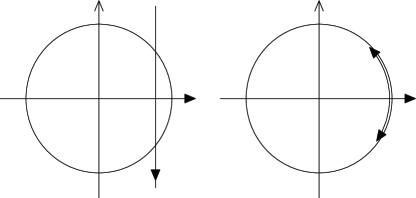
Figure 1: A straight motion with $m_{R}=\Lambda+ig\varphi$ is shown in the left, and the rotational oscillation with $m_{R}=|m_{R}|e^{i\theta(t)}$ is shown in the right.

III Particle production due to the background oscillations

Our next topic is the nonequilibrium particle production in a more realistic scenario. To compare our results with the conventional spontaneous baryogenesis, we first review the calculation given in Ref.Dolgov:1996qq . They have considered the Lagrangian density

$${\cal L} = \partial_{\mu}\Phi^{*}\partial^{\mu}\Phi-V(\Phi^{*}\Phi)$$ (66)

$$+i\bar{Q}(i\gamma^{\mu}\partial_{\mu}-m_{Q})Q+\bar{L}(i\gamma^{\mu}\partial_{\mu}-m_{L})L$$

$$+\left(g\Phi\bar{Q}L+H.c.\right),$$

which has the $U(1)$ symmetry corresponding to baryon number

$$\Phi\rightarrow e^{i\alpha}\Phi, Q\rightarrow e^{-i\alpha}Q, L\rightarrow L.$$ (67)

Defining $\langle\Phi\rangle=fe^{i\theta}/\sqrt{2}$, one obtains an effective Lagrangian density

$${\cal L} = \frac{f^{2}}{2}\partial_{\mu}\theta\partial^{\mu}\theta$$ (68)

$$+i\bar{Q}(i\gamma^{\mu}\partial_{\mu}-m_{Q})Q+\bar{L}(i\gamma^{\mu}\partial_{\mu}-m_{L})L$$

$$+\left(\frac{ge^{i\theta}}{\sqrt{2}}f\bar{Q}L+H.c.\right).$$

$\theta$ in the above Lagrangian is the Nambu-Goldstone boson. Considering the rotation

$$Q\rightarrow e^{-i\alpha}Q, L\rightarrow L, \theta\rightarrow\theta+\alpha$$ (69)

and assigning $\alpha=-\theta$, the Lagrangian gives

$${\cal L} = \frac{f^{2}}{2}\partial_{\mu}\theta\partial^{\mu}\theta$$ (70)

$$+i\bar{Q}(i\gamma^{\mu}\partial_{\mu}-m_{Q})Q+\bar{L}(i\gamma^{\mu}\partial_{\mu}-m_{L})L$$

$$+\left(\frac{g}{\sqrt{2}}f\bar{Q}L+H.c.\right)+\partial_{\mu}\theta J^{\mu},$$

where $J^{\mu}=\bar{Q}\gamma^{\mu}Q$.

In the above, we have followed Ref.Dolgov:1996qq and rotated $Q$ to remove the phase. However, one will soon find that the assignment of the rotation is not unique. Actually, if one rotates the fields as

$$Q\rightarrow e^{i\alpha^{\prime}(x)}Q, L\rightarrow e^{i\alpha^{\prime}(x)}L,$$ (71)

the phases in the interaction remain the same. On the other hand, one will find that

$$\mathcal{L}_{\rm add}=-\partial_{\mu}\alpha^{\prime}\cdot(\bar{Q}\gamma^{\mu}Q+\bar{L}\gamma^{\mu}L)$$ (72)

appears. This term is related to the (global) $U(1)_{B+L}$ in the original Lagrangian. Choosing $\partial_{t}\alpha^{\prime}\neq 0$, the chemical potential appears for the net $B+L$ number. Therefore, if the task is just to remove the phase in the interaction, the definition of the rotation (and of course the chemical potential) has the ambiguity. This is not a surprise. If one can use the relation $(n_{Q}-\bar{n}_{Q})+(n_{L}-\bar{n}_{L})=0$, one can always rewrite the chemical potential as $\mu(n_{Q}-\bar{n}_{Q})\rightarrow\frac{\mu}{2}(n_{Q}-\bar{n}_{Q})-\frac{\mu}{2}(n_{L}-\bar{n}_{L})$, where $\mu$ is $Q$’s chemical potential. In the thermal equilibrium, the chemical potential has to balance.

Besides the symmetry discussed above, the Lagrangian is symmetric under the exchange $\{L\leftrightarrow Q,\Phi\leftrightarrow\Phi^{*}\}$. Assuming that the Berry transformation respects this symmetry, the transformation has to be $Q\rightarrow e^{i\theta/2}Q$ and $L\rightarrow e^{-i\theta/2}L$ without ambiguity.

Using the calculation in Sec. II.2, we can calculate the asymmetries, which appear both for $Q$ and $L$ with the opposite signs.

The above arguments seem to be suggesting that the assignment $Q\rightarrow e^{i\theta/2}Q,\quad L\rightarrow e^{-i\theta/2}L$ is more natural. On the other hand, if one assumes that the coefficients are determined by the $U(1)$ symmetry given by Eq.(67), and claims that the chemical potential is appearing form the derivative coupling of the Nambu-Goldstone boson of the broken symmetry, the assignment seems to be unique.

Now consider the particle production in the time-dependent and nonequilibrium background. The production can be biased by the oscillation given by

$$\Phi(t) = fe^{i\theta(t)},$$

$$\theta(t) = \theta_{i}e^{-\Gamma t/2}\cos{m_{\theta}t}.$$ (73)

Expanding $\theta$ for small $\theta$ as

$$e^{i\theta(t)}=1+i\theta(t)-\theta(t)^{2}/2,$$ (74)

one will findDolgov:1996qq

$$\Delta n_{Q}\equiv n_{Q}-\bar{n}_{Q} = \frac{g^{2}}{16\pi}m_{\theta}f^{2}\theta_{i}^{3}.$$ (75)

Note, however, that the above expansion of $e^{i\theta}$ already ruins the original symmetry. Is the violation of the symmetry crucial for the asymmetry? We will solve this problem in Sec. III.4 using the formalism of the Berry phase.

III.1 Small extension and the perturbative expansion

To check the validity of the above calculation in wider circumstances, let us remove the condition

$$\Phi(t) = fe^{i\theta(t)},$$ (76)

and consider the interaction replaced by

$$g\Phi(t) \rightarrow \Lambda+g\varphi(t),$$ (77)

where $\Lambda$ is real but $g$ is a complex constant, and $\varphi(t)$ is a time-dependent real scalar field. Later, we will discuss the nonperturbative particle production, but in this section we are confined to the perturbative expansion. As is shown in Ref.Dolgov:1996qq , the average number density $n$ of particle(or antiparticle) pairs produced by the decay of a homogeneous classical scalar field can be calculated as

$$\Delta n_{Q} = \frac{1}{\pi^{2}}\int d\omega\omega^{2}\left|\int^{\infty}_{-\infty}dte^{2i\omega t}(\Lambda+g\varphi)\right|^{2}$$ (78)

$$-\frac{1}{\pi^{2}}\int d\omega\omega^{2}\left|\int^{\infty}_{-\infty}dte^{2i\omega t}(\Lambda+g^{*}\varphi)\right|^{2},$$

where $2\omega=p_{a}^{0}+p_{b}^{0}$ is for the particle pair $a$ and $b$.

Using $g=g_{R}+ig_{I}$, one can expand $(\Lambda+g\varphi)$ as

$$(\Lambda+g\varphi) = \Lambda+ig_{I}\varphi+g_{R}\varphi.$$ (79)

The cross term that may give a nonzero contribution to the baryon asymmetry is

$$\Delta n_{Q} = \frac{2}{\pi^{2}}\int d\omega\omega^{2}\left[if_{I}f^{*}_{R}+h.c.\right],$$

$$f_{I} = \int^{\infty}_{-\infty}dte^{2i\omega t}g_{I}\varphi(t)$$

$$f_{R} = \int^{\infty}_{-\infty}dte^{2i\omega t}g_{R}\varphi(t).$$ (80)

Here we assume that the oscillation starts at $t=0$ and $\varphi(t)$ is given by

$$\varphi(t) = \varphi_{i}e^{-\Gamma t/2}\cos{mt},$$ (81)

where $\Gamma$ and $m$ are a decay rate and a mass of $\varphi$ field. We can calculate the integral, which is given by

$$f_{I(R)} = \frac{g_{I(R)}\theta_{i}}{4i\omega}\left[\frac{-\Gamma/2+im}{-\Gamma/2+im+2i\omega}\right.$$ (82)

$$+\left.\frac{-\Gamma/2-im}{-\Gamma/2-im+2i\omega}\right].$$

Since $[if_{I}f_{R}^{*}+H.c]=0$ is obvious in this case, the final result becomes

$$\Delta n_{Q} = 0,$$ (83)

which suggests that there is no asymmetry generation. We already know that in the conventional baryogenesis scenario one has to consider multiple (quantum) corrections to generate the required interference. We can see that the same thing is happening in this perturbative calculation. (On the other hand, the same interaction can generate the asymmetry in the nonperturbative limit. We will discuss this issue in Sec. III.5 for the Majorana fermions.)

III.2 Higher terms for the perturbative expansion

To avoid the cancellation, or to introduce interference between multiple contributions, one can introduce higher terms. For instance, one can introduce

$$g\Phi(t) \rightarrow \Lambda+g_{1}\varphi+g_{2}\frac{\varphi^{2}}{M_{*}},$$ (84)

where both $g_{1}$ and $g_{2}$ are complex. Note that this is no longer giving the approximation of the rotational oscillation. In the simplest case, $m_{R}$ can be written as

$$g\Phi(t) \rightarrow \Lambda+i\lambda_{1}\varphi-\frac{\lambda_{2}}{2}\frac{\varphi^{2}}{M_{*}},$$ (85)

where $\lambda_{i}$ is a real constant. Following the calculation in Ref.Dolgov:1996qq , we find the asymmetry given by

$$n_{\nu}-\bar{n}_{\nu} = \frac{1}{16\pi}m\Lambda^{2}\left(\frac{\lambda_{1}\lambda_{2}\varphi_{i}^{3}}{\Lambda^{2}M_{*}}\right)$$ (86)

$$= \frac{\lambda_{1}\lambda_{2}}{16\pi}mM_{*}^{2}\left(\frac{\varphi_{i}}{M_{*}}\right)^{3}.$$

Although the above calculations are useful for understanding the origin of the asymmetry, the model is a trivial extension of Ref.Dolgov:1996qq . The only difference is that the terms are not approximating the rotation.

In the followings, we will consider the Dirac and the Majorana fermions and examine the origin of the asymmetry in the nonperturbative particle production.

III.3 The Dirac mass for the nonperturbative calculation

Usually, the Dirac mass is defined to be real since the redefinition of the field can remove the phase. However, if the Dirac mass is time dependent, the Berry connection appears. Let us introduce the complex Dirac mass, which is rotating with $m_{D}(t)\equiv M_{D}e^{i\theta(t)}$. The phase can be removed by defining the Berry transformation for the left and the right-handed fermions. In the equation of motion, $\dot{\theta}\neq 0$ introduces asymmetry of the helicity for each (matter and antimatter) state, but we will show that there is no asymmetry in the total number densities. Since the asymmetry is due to the violation of the time-reversal symmetry by the background, our expectation is that the asymmetry is due to the shifts of the “events” of the particle production.

To show that our expectation is correct, we start with a simple example. Since the basic idea of the fermionic preheating has already been discussed in Refs.Dolgov:1989us ; Greene:1998nh ; Chung:1999ve ; Peloso:2000hy , we are going to follow the notations of Ref.Peloso:2000hy . The new ingredient of our calculation is the complex Dirac mass

$$m_{D}(t) = i\Lambda+g\varphi(t),$$ (87)

where $g$ is real. Note that we are not considering a simple circular rotation but a straight motion, whose orbit is (slightly) shifted from the origin and introduces significant $\dot{\theta}\neq 0$ when it passes near the origin. Considering the decomposition

$$\psi = \int\frac{d^{3}k}{(2\pi)^{3}}e^{-i\bm{k}\cdot\bm{x}}\sum_{s}\left[u^{s}_{\bm{k}}(t)a^{s}_{\bm{k}}+v^{s}_{\bm{k}}(t)b^{s\dagger}_{-\bm{k}}\right]$$ (88)

for the Dirac equation

$$(i\not{\partial}-m_{D})\psi = 0,$$ (89)

one will find

$$\dot{u}_{\pm} = iku_{\mp}\mp im_{D}u_{\pm},$$ (90)

which can be decoupled into

$$\ddot{u}_{\pm}+\left[\omega^{2}\pm i\dot{m}_{D}\right]u_{\pm},$$ (91)

where $\omega(t)^{2}=k^{2}+|m_{D}|^{2}$. Let us consider the evolution equation near the bottom, $\varphi(t_{*})=0$. If we write

$$\varphi(t) \simeq \dot{\varphi}_{*}(t-t_{*}),$$ (92)

where $\dot{\varphi}_{*}$ is a constant defined at $t=t_{*}$, the equation of motion gives

$$\ddot{u}_{\pm}+\left[k^{2}+|i\Lambda+g\dot{\varphi}_{*}(t-t_{*})|^{2}\pm ig\dot{\varphi}_{*}\right]u_{\pm}=0.$$ (93)

Obviously, the above Dirac mass $m_{D}(t)$ does not introduce a new parameter, which might distinguish $u_{\pm}$. Therefore, the above simplest extension does not introduce asymmetry during the particle production. This result reminds us of the perturbative production considered in the model of $Q$ and $L$.

To introduce the asymmetry, we consider the higher term, which is given by

$$m_{D}(t) = i\Lambda+g_{1}\varphi+ig_{2}\frac{\varphi^{2}}{M_{*}},$$ (94)

where $\Lambda,g_{1},g_{2}$ are taken to be real. Then the equation of motion gives

$$\ddot{u}_{\pm}+\left[k^{2}+\left|i\Lambda+g_{1}\dot{\varphi}_{*}(t-t_{*})+ig_{2}\frac{\dot{\varphi}^{2}}{M_{*}}(t-t_{*})^{2}\right|^{2}\right.$$

$$\left.\pm\left(ig_{1}\dot{\varphi}_{*}-2g_{2}\frac{\dot{\varphi}^{2}}{M_{*}}(t-t_{*})\right)\right]u_{\pm}=0.$$ (95)

Note that the asymmetry appears in the real part in the bracket. Introducing new parameters

$$A \equiv \dot{\varphi}^{2}\left(g_{1}^{2}+2g_{2}\frac{\Lambda}{M_{*}}\right)$$

$$B \equiv \dot{\varphi}^{2}\left(\frac{g_{2}}{M_{*}}\right),$$ (96)

and disregarding $(t-t_{*})^{4}$ near $t=t_{*}$, one can rewrite the equation as

$$\ddot{u}_{\pm}+\left[k^{2}+\Lambda^{2}+A(t-t_{*})^{2}\mp 2B(t-t_{*})\pm ig_{1}\dot{\varphi}_{*}\right]u_{\pm}=0.$$

Defining $t_{\pm}\equiv t_{*}\pm B/A$ and

$$\omega_{\pm}^{2} \equiv k^{2}+\Lambda^{2}-B^{2}/A+A(t-t_{\pm})^{2}>0,$$ (98)

we have

$$\ddot{u}_{\pm}+\left[\omega_{\pm}^{2}\pm ig\dot{\varphi}_{*}\right]u_{\pm}=0.$$ (99)

Now the calculation of the number densities is straightforward; the above equation is almost identical to the standard equationPeloso:2000hy , except for the helicity-dependent $\omega_{+}\neq\omega_{-}$. The split of $t_{*}$ into $t_{\pm}$ ($t_{+}>t_{*}>t_{-}$) means that the production of $u_{-}$ begins earlier than $u_{+}$. This is due to the modification of the real part in the bracket in Eq.(III.3). Although the nonadiabatic areas are partially overlapping, as is shown in Fig.2, it is possible to expect that the (earlier) production of $u_{-}$ is so significant that it reduces $\dot{\varphi}$ before the (later) production of $u_{+}$. In this case, one has to define $\varphi(t)_{\pm}\simeq\dot{\varphi}_{\pm}(t-t_{\pm})$ for each $u_{\pm}$. In the most significant case, where one can assume that almost all the states in the Fermi sphere are occupied, $(|\dot{\varphi}_{+}|<|\dot{\varphi}_{-}|)$ determines the asymmetry of the maximum $|\bm{k}|$ of each Fermi sphere.

For the antimatter state, the decoupled equation(91) has $\dot{m}_{D}^{*}$ instead of $\dot{m}_{D}$. Therefore, we find $t_{\pm}\equiv t_{*}\mp B/A$ for the antimatter, which is opposite to the matter, and gives $n_{\pm}=\bar{n}_{\mp}$. In total, there is no asymmetry because $n_{+}+\bar{n}_{+}=n_{-}+\bar{n}_{-}$ is always satisfied, even though $n_{+}\neq n_{-}$ and $\bar{n}_{+}\neq\bar{n}_{-}$ are possible in this case.

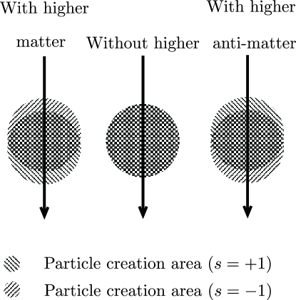
Figure 2: Particle creation area (nonadiabatic area) for $m_{D}=i\Lambda+g\varphi(t)$ is shown in the middle. In both sides, matter and antimatter creation for $m_{R}=i\Lambda+g_{1}\varphi+ig_{2}\frac{\varphi^{2}}{M_{*}}$ is shown. In the left, $s=-1$ creation starts earlier than $s=+1$, while in the right, $s=+1$ creation starts earlier than $s=-1$.

To conclude the particle production due to the Dirac mass, there is no total asymmetry even if the higher terms are introduced. The asymmetry of the helicity appears for each (matter and antimatter) state because the event of the particle production splits. Similarly, the matter-antimatter asymmetry appears for each helicity state. However, these partial asymmetries do not cause generation of the total asymmetry.

To avoid the cancellation of the asymmetries, which has been seen for the Dirac mass, we will consider the Majorana fermion in the followings. Note that unlike the Dirac fermion, decoupling of the equations is not well-defined at the massless point. First, we consider the rotational oscillation and compare the perturbative and the non-perturbative particle production. Then we examine the nonrotational motion. We will show that unlike the previous models the asymmetry can be generated without introducing the higher terms.

III.4 Majorana fermion for the rotational oscillation

In this section, we consider simple oscillation of $\theta$ for the Majorana fermion mass. Using $\Psi^{t}_{R}\equiv(\psi_{R},\psi_{L}^{c})$, one can write the Majorana mass term as

$${\cal L}_{m} = \bar{\Psi}_{R}\left(\begin{array}[]{cc}0&m_{R}\\ m_{R}^{*}&0\end{array}\right)\Psi_{R},$$ (102)

where we consider $m_{R}(t)=M_{R}e^{i\theta(t)}$. Remember that in Sec. III.2, we have calculated the asymmetry using the expansion $e^{i\theta}=1+i\theta+...$. However, the problem is that the expansion is obviously violating the original symmetry of the rotation. To solve this problem, we calculated the asymmetry generation using the Berry transformation. The calculational details are shown in Appendix A. The calculation uses the Yang-Feldman formalism and the Berry transformation. Thanks to the Berry transformation, we do not have to use the expansion $e^{i\theta(t)}=[1+i\theta-\theta^{2}/2+...]$. Our result shows that the asymmetry appears from the third order of the perturbative expansion. Taking the limit $m_{\theta}\gg|m_{\xi}|\gg\Gamma$, our result gives the previous calculation, which is given by

$$n_{\nu}-\bar{n}_{\nu} \sim \frac{1}{4\pi}|m_{R}|^{2}m_{\theta}\theta_{i}^{3},$$ (103)

where $\theta_{i}$ is an initial phase of the mass. This result is similar to (75) if one regards $|m_{R}|$ as $gf$, which is a mixing mass term between $Q$ and $L$ in (70). Note that our calculation takes into the poles shifted by $\Gamma$.

To understand more about the sources of the asymmetry, we will consider the non-perturbative effect (tunneling) using another schematic calculation. We use the Lagrangian given by

$${\cal L} = \bar{\psi}_{R}i\bar{\sigma}^{\mu}\partial_{\mu}\psi_{R}+\left(m_{R}\bar{\psi_{L}^{c}}\psi_{R}+m_{R}^{*}\bar{\psi_{R}}\psi_{L}^{c}\right).$$ (104)

The equation of motion is

$$(i\partial_{t}-i\bm{\sigma}\cdot\bm{\partial})\psi_{R} = -m_{R}^{*}\psi_{L}^{c}.$$ (105)

We expand

$$(\psi_{R})_{\alpha} = \int\frac{d^{3}k}{(2\pi)^{3}}e^{i\mathbf{k\cdot x}}\sum_{s=\pm}(e^{s}_{\bm{k}})_{\alpha}$$ (106)

$$\times\left[u^{s}_{k}(x^{0})a^{s}_{\bm{k}}+sv^{s}_{\bm{k}}(x^{0})a_{-\bm{k}}^{s\dagger}\right],$$

where $e_{\mathbf{k}}^{s}$ is the eigenstate of the helicity operator, which gives

$$-k^{i}\bar{\sigma}^{i}e_{\mathbf{k}}^{s}=s|\mathbf{k}|\bar{\sigma}^{0}e_{\mathbf{k}}^{s}.\qquad(s=\pm)$$ (107)

Substituting this expansion into the equation of motion, we find

$$(i\partial_{t}+s|\bm{k}|)u^{s}_{\bm{k}}=sm_{R}^{*}v^{s}_{\bm{k}},$$

$$(i\partial_{t}+s|\bm{k}|)v^{s*}_{\bm{k}}=-sm_{R}^{*}u^{s*}_{\bm{k}}.$$ (108)

Unlike the Dirac fermions, the coefficients of the mixing terms (in the right-hand side) are depending on time. Therefore, to decouple the equations, one has to remove the time dependence. After removing the time dependence using the Berry transformation, one will find the chemical potential and the constant Majorana mass. The equations can be solved by using the conventional decoupling. Here, we are not going to decouple the equations.

This equation can be written as

$$i\frac{d}{dt}\Psi = H\Psi,$$

$$\left(\begin{array}[]{cc}H_{11}&H_{12}\\ H_{21}&H_{21}\end{array}\right) = \left(\begin{array}[]{cc}-s|\bm{k}|&sm_{R}^{*}(t)\\ sm_{R}(t)&s|\bm{k}|\end{array}\right),$$ (113)

where $\Psi^{t}\equiv(v^{s}_{\bm{k}},u^{s}_{\bm{k}})$. For the simple rotational oscillation, we consider

$$m_{R}(t)=M_{R}e^{i\theta(t)}, \theta(t)=\theta_{0}\cos m_{\theta}t.$$ (114)

After the Berry transformation, we find

$$i\frac{d}{dt}\psi^{R} = \hat{H}^{R}\psi^{R},$$

$$\hat{H}^{R} = \left(\begin{array}[]{cc}-s|\bm{k}|+\frac{\theta_{0}m_{\theta}}{2}\sin m_{\theta}t&sM_{R}\\ sM_{R}&s|\bm{k}|-\frac{\theta_{0}m_{\theta}}{2}\sin m_{\theta}t\end{array}\right).$$ (117)

The above equation reminds us of the Landau-Zener tunnelingZener:1932ws .

Figure 3: The top figure shows the original Landau-Zener tunneling. Eq.(121) for $s=\pm$ is shown in the bottom. There is the shift of the oscillation due to the sign of the helicity. The tunneling occurs when $-s|\bm{k}|+\frac{\theta_{0}^{s(i)}m_{\theta}}{2}\sin m_{\theta}t_{\bm{k}}^{s(i)}=0$. From the picture, we can find the relation $t_{\bm{k}}^{+(i)}\simeq t_{\bm{k}}^{-(i)}+\frac{\pi}{m_{\theta}}$, which is exact when the amplitude does not change with time.

Following Ref.Zener:1932ws , we can define

$$\left(\begin{array}[]{cc}\epsilon_{1}&\epsilon_{12}\\ \epsilon_{21}&\epsilon_{2}\end{array}\right)$$ (121)

$$= \left(\begin{array}[]{cc}-s|\bm{k}|+\frac{\theta_{0}m_{\theta}}{2}\sin m_{\theta}t&sM_{R}\\ sM_{R}&s|\bm{k}|-\frac{\theta_{0}m_{\theta}}{2}\sin m_{\theta}t\end{array}\right),$$ (124)

which is shown in Fig.3 together with the original Landau-Zener tunneling. The probability of the translation at each crossing point is given by

$${\cal P}_{\bm{k}}^{s(i)} \simeq e^{-\pi p^{s(i)}_{\bm{k}}},$$

$$p_{\bm{k}}^{s(i)} \equiv \frac{M_{R}^{2}}{\left|\frac{\theta_{0}^{s(i)}m_{\theta}^{2}}{2}\cos m_{\theta}t_{\bm{k}}^{s(i)}\right|},$$ (125)

where $t_{\bm{k}}^{s(i)}$ for the ith event is defined by

$$-s|\bm{k}|+\frac{\theta_{0}^{s(i)}m_{\theta}}{2}\sin m_{\theta}t_{\bm{k}}^{s(i)} = 0.$$ (126)

Substituting Eq.(126) into Eq.(III.4), we find

$$p_{\bm{k}}^{s(i)} \equiv \frac{2M_{R}^{2}}{m_{\theta}^{2}\theta_{0}^{s(i)}}\left(1-\frac{4|\bm{k}|^{2}}{m_{\theta}^{2}(\theta_{0}^{s(i)})^{2}}\right)^{-1/2},$$ (127)

where $|\bm{k}|<\theta_{0}^{s(i)}m_{\theta}/2$ is required for the tunneling. Using the conventional Bogoliubov transformation, the total number density can be calculated as

$$n^{s}_{\bm{k}} \simeq \sum_{i}{\cal P}_{\bm{k}}^{s(i)},$$ (128)

where particles are assumed to decay before the next particle production. One can verify that the above result is consistent with Refs.Peloso:2000hy ; Adshead:2015kza , in which the Landau-Zener tunneling has not been used for the calculation. Since $m_{\theta}$ is the mass of $\theta$ appearing in $m_{R}=M_{R}e^{i\theta}$, the limit $M_{R}\ll m_{\theta}$ is unlikely in this model. Note also that the equation becomes singular in the limit $M_{R}\rightarrow 0$ (See Ref.Zener:1932ws ).

Let us temporarily assume that the amplitude $\theta_{0}$ is constant within a cycle. Then, one can see that the same particle creation is occurring for each helicity state, but they do not happen simultaneously. From Fig.3, one can see that the particle creation is delayed for the helicity state $s=-1$, and the delay is just a half of the oscillation time.

When the amplitude decreases with time, the delay is approximately given by $\Delta t\simeq\frac{\pi}{m_{\theta}}$. Then, if the amplitude behaves like $\propto e^{-\Gamma t}$, the amplitude $\theta_{0}^{s(i)}$ defined for the ith event can be expressed as

$$\theta_{0}^{-(i)} \simeq e^{-\Gamma\Delta t}\theta_{0}^{+(i)}.$$ (129)

In this case, the origin of the asymmetry is $\theta_{0}^{-(i)}\neq\theta_{0}^{+(i)}$, which directly biases $p_{\bm{k}}^{s(i)}$ in Eq.(127). Therefore, we can clearly understand that the time-dependent amplitude is the source of the asymmetry in this case.

From Eq.(127), one can see that $p_{\bm{k}}^{s(i)}$ can be approximated as a constant within $|\bm{k}|<k_{Max}^{(i)}\equiv\theta_{0}^{s(i)}m_{\theta}/2$. If one assumes $p_{\bm{k}}^{s(i)}\sim 1$ within $|\bm{k}|<k_{Max}$, the asymmetry becomes

$$n_{+}^{(i)}-n^{(i)}_{-} \propto (k^{(i)}_{Max})^{2}\frac{dk^{(i)}_{Max}}{d\theta_{0}^{+}}d\theta_{0}^{+}$$ (130)

$$\sim m_{\theta}^{2}\Gamma(\theta_{0}^{+(i)})^{3},$$

where we expanded

$$\theta_{0}^{-(i)} \simeq \left(1-\frac{\pi\Gamma}{m_{\theta}}\right)\theta_{0}^{+(i)}.$$ (131)

Here, we assumed that $\Gamma\propto m_{\theta}$ and $\Gamma\Delta t\simeq\frac{\pi\Gamma}{m_{\theta}}\ll 1$.

III.5 Majorana Fermions for the simplest extension

Instead of considering the rotational motion, we are going to introduce the Majorana mass given by

$$m_{R}(t) = i\Lambda+g\varphi(t),$$ (132)

where (just for simplicity) both $\Lambda$ and $g$ are taken to be real. Previously, we have seen that the above extension (without higher terms) does not generate the asymmetry for the perturbative calculation.

In this section, using the non-perturbative calculation, we will show that the above extension can generate the asymmetry. We consider significant particle production, which is realized when the oscillation starts with $|\Lambda/g\varphi|\ll 1$. Again, we use the Lagrangian given by Eq.(104). To decouple the equation of motion (III.4) for $\dot{m}_{R}\neq 0$, we rewrite the equation as

$$(m_{R}^{*})^{-1}(i\partial_{t}+s|\bm{k}|)u^{s}_{\bm{k}}=sv^{s}_{\bm{k}},$$ (133)

and obtain

$$(-i\partial_{t}+s|\bm{k}|)\left[(m_{R}^{*})^{-1}(i\partial_{t}+s|\bm{k}|)u^{s}_{\bm{k}}\right]$$ (134)

$$= \left[\frac{\partial_{t}^{2}+|\bm{k}|^{2}}{m_{R}^{*}}+i\frac{\dot{m}_{R}^{*}}{m_{R}^{*2}}(i\partial_{t}+s|\bm{k}|)\right]u^{s}_{\bm{k}}$$

$$= -m_{R}u^{s}_{\bm{k}}.$$

Therefore, one obtains the decoupled equation

$$\left[\partial_{t}^{2}-\frac{\dot{m}_{R}^{*}}{m_{R}^{*}}\partial_{t}+|\bm{k}|^{2}+is|\bm{k}|\frac{\dot{m}_{R}^{*}}{m_{R}^{*}}\right]u^{s}_{\bm{k}} = -|m_{R}|^{2}u^{s}_{\bm{k}}.$$

Substituting

$$u_{\bm{k}}^{s} = e^{\int\frac{\dot{m}_{R}^{*}}{2m_{R}^{*}}dt}U_{\bm{k}}^{s},$$ (136)

we find

$$\ddot{U}_{\bm{k}}^{s}+\left[\dot{\left(\frac{\dot{m}_{R}^{*}}{m_{R}^{*}}\right)}-\frac{1}{4}\left(\frac{\dot{m}_{R}^{*}}{m_{R}^{*}}\right)^{2}+|\bm{k}|^{2}+|m_{R}|^{2}+is|\bm{k}|\frac{\dot{m}_{R}^{*}}{m_{R}^{*}}\right]U$$ (137)

$$=0$$ .

From this equation, one can immediately understand that the asymmetric particle production is possible in this case. If we define $v\equiv g\dot{\phi}(t_{*})$, $g\varphi(t)=v(t-t_{*})$ near the bottom of the oscillation, we have

$$\frac{\dot{m}_{R}^{*}}{m_{R}^{*}}\simeq\frac{v}{i\Lambda}, \dot{\left(\frac{\dot{m}_{R}^{*}}{m_{R}^{*}}\right)}\simeq\frac{v^{2}}{\Lambda^{2}}$$ (138)

Then, for $t_{*}=0$, we can write the equation as

$$\ddot{U}_{\bm{k}}^{s}+\left[\frac{5}{4}\frac{v^{2}}{\Lambda^{2}}+|\bm{k}|^{2}+\Lambda^{2}+v^{2}t^{2}+s|\bm{k}|\left(\frac{v}{\Lambda}\right)\right]U = 0.$$

Defining

$$|\bm{\hat{}}{k}^{s}| \equiv |\bm{k}|+\frac{s}{2}\frac{v}{\Lambda},$$ (140)

we obtain

$$\ddot{U}_{\bm{k}}^{s}+\left[|\bm{\hat{}}{k}^{s}|^{2}+m_{eff}^{2}(t)\right]U = 0,$$ (141)

where

$$m_{eff}^{2}(t)\equiv\frac{v^{2}}{\Lambda^{2}}+\Lambda^{2}+v^{2}t^{2}.$$ (142)

Therefore, when $\Lambda^{2}\ll v$, particle production is not significant near the bottom. The simplest assumption, which justifies the significant particle production, is $\Lambda\sim v^{1/2}$. The equation is almost the same as the conventional preheating, except for the helicity-dependent $|\bm{\hat{}}{k}^{s}|^{2}$. We can conclude that the asymmetry is due to the split of $|\bm{\hat{}}{k}^{s}|^{2}$. During the particle production, it shifts the radius of the Fermi sphere of each helicity state.

Unlike the perturbative expansion discussed in Sec. III.1, our non-perturbative calculation gives the asymmetry. Basically, the perturbative expansions and the non-perturbative effects (such as the tunnelings) will give different contributions. These are expected to be unified in the resurgence theoryDelabaere:1999 ; Dorigoni:2014hea . Since the basic equations are written in ordinary differential equations (ODEs), one can use the resurgence of ODEs, which has already been solved in the mathematical side. The task is to identify the origin of the asymmetry in the framework of the resurgence. Note that $i\Lambda\rightarrow-i\Lambda$ flips the asymmetry and there is a singularity at $\Lambda=0$. The relation will be revealed in our next paper.

III.6 Comment on a more ambitious approach: Multifield extension and the Cabibbo-Kobayashi-Maskawa matrix

In the above models, the source of the phase is designed to be very simple. The phase in the off-diagonal element determines the Berry phase, and there is the obvious correspondence between them. We have also seen that a simple extension of the scenario (i.e, $\Delta=\Lambda+ig\varphi$) can be used to generate the effective chemical potential. In this case, there is no obvious correspondence between the Berry phase and the phases of the “fundamental” parameters $\Lambda,g$, and $\varphi$. However, generation of the effective chemical potential is very clear in the light of the Berry transformation.

In the above models, all phases in the Hamiltonian can be removed by the field rotation, which we called “the Berry transformation.” Now our question is very simple. “What happens if the fields are multiplied and the Berry transformation has to be given by a complex function of the original parameters?”

One can examine the above idea in the three-family fermion model. One can introduce the flavor index $i=1,2,3$ and write

$${\cal L} = i\bar{Q}_{i}(i\gamma^{\mu}\partial_{\mu}-m_{Q}^{ij})Q_{j}+\bar{L}_{i}(i\gamma^{\mu}\partial_{\mu}-m_{L}^{ij})L_{j}$$ (143)

$$+\left(f^{ij}\bar{Q}_{i}L_{j}+H.c.\right),$$

where $m_{Q},m_{L}$ can be diagonalized by unitary transformations where $\hat{Q}_{i}=(U_{Q}^{\dagger})^{ij}Q_{j},\hat{L}_{i}=(U_{L}^{\dagger})^{ij}L_{j}$. Then the interaction is written as

$${\cal L}_{int} = \left((U_{Q}^{\dagger}fU_{L})^{ij}\bar{\hat{Q}}_{i}\hat{L}_{j}+H.c.\right).$$ (144)

Now the CP phase appearing in the matrix $V^{ij}\equiv(U_{Q}^{\dagger}fU_{L})^{ij}$ is quite similar to the famous Cabibbo-Kobayashi-Maskawa matrix in the standard model. Unlike the naive $2\times 2$ matrix models we have considered previously, the phases in $V^{ij}$ are not simply determined by the complex phases of the original parameters of the Lagrangian. (To avoid confusions, note that we have considered only the single flavor for the Q-L model. $2\times 2$ matrix was considered for the kaonlike models and the Majorana fermions, but the matrix was for the matter and the antimatter, not for the flavor.) The phases in $V^{ij}$ are given by the functions of all the original parameters. Therefore, even if the time-dependent motion does not accompany any rotation of the original complex parameter, the motion may introduce time-dependent phases in $V^{ij}$, which can eventually introduce the chemical potential in the Hamiltonian through the Berry connection. Note that usually the phases in $V^{ij}$ are removed by the field rotations and only a CP phase (Kobayashi-Maskawa CP phase) remains.

The minimal multifield extension that realizes the above idea is given by a complex scalar field couples to a real scalar field. Consider the following Lagrangian;

$${\cal L} = |\partial_{\mu}\phi|^{2}-m_{\phi}^{2}|\phi|^{2}$$ (145)

$$+\frac{1}{2}(\partial_{\mu}\eta)^{2}-\frac{1}{2}m_{\eta}^{2}\eta^{2}$$

$$-\frac{1}{2}(\epsilon\phi^{2}+H.c.)-(g\phi+H.c)\eta,$$

where $\phi$ is a complex scalar and $\eta$ is a real scalar. Here, $\epsilon$, $g$ are complex coupling constants. Note that in this case the complex phases of $\epsilon$ and $g$ are not removed simultaneously by the field rotation. Therefore, at least one complex phase will remain “after” the field rotation. The equations of motion are given by

$$\ddot{\Psi}^{R}+\Omega^{2}\Psi^{R}=0$$ (146)

where

$$\Psi^{R}\equiv\left(\begin{array}[]{cc}\phi\\ \phi^{\dagger}\\ \eta\end{array}\right),\quad\Omega^{2}\equiv\left(\begin{array}[]{ccc}\omega_{\phi}^{2}&\epsilon_{R}&g^{*}\\ \epsilon_{R}&\omega_{\phi}^{2}&g\\ g&g^{*}&\omega_{\eta}^{2}\end{array}\right).$$ (147)

Here, $\epsilon_{R}$ is set real but $g$ is still a complex parameter. Note that we have already used the field rotation of $\phi$ to have $\epsilon_{R}$. To diagonalize the matrix using a unitary matrix $U$, one has to calculate eigenvectors of the matrix $\Omega^{2}$. Because $\Omega^{2}$ has a complex element, the unitary matrix must also have complex elements. Here, the key idea is that the unitary matrix can be decomposed using (real) rotation and complex matricesKobayashi:1973fv , which are sometimes denoted as $U_{12},U_{13},U_{23}$ and $U_{\theta_{i}}$. Since the particle production occurs for the eigenstates, one has to consider $\Psi^{E}$, which is given by the transformation using $U_{12},U_{13},U_{23}$ and $U_{\theta_{i}}$. In Ref.Enomoto:2017rvc , we have shown that the “eigenstates” are preserving matter-antimatter asymmetry but they are mixed by the Berry connection. In this case, the phases in the Berry transformation are functions of $\omega_{\phi},\epsilon_{R},\omega_{\eta}$ and $g$. Therefore, in this model, one can expect that a time-dependent $\omega_{\phi}$ can generate matter-antimatter asymmetry, since it may change the phase parameter as $\dot{\theta}_{i}=\dot{\omega}_{\phi}(\partial\theta_{i}/\partial\omega_{\phi})$. Note that $\omega_{\phi}$ itself does not have a phase, which is similar to the simple extension discussed in Sec. II.3. The analytic relation between the chemical potential and $\dot{\omega}_{\phi}$ has a very lengthy form, since it uses the eigenvectors of the $3\times 3$ matrix $\Omega^{2}$. In Ref.Enomoto:2017rvc , we showed a numerical calculation to show that the matter-antimatter asymmetry is generated in this model. Viewing with the “eigenstates”($\Psi^{E}$), the Berry connection causes mixing between “eigenstates” accompanied by the CP phase, which is time dependent, to generate the interference between states.

IV The Berry phase and the Legendre transformation

The chemical potential may cause a problem in the Legendre transformation if it is explained by the derivative coupling of a field in motion. The reason is very simple. If the chemical potential is introduced using the derivative of the field $\phi$, the Lagrangian density acquires the term

$${\cal L}_{c} = (\partial_{\mu}\phi)J^{\mu}_{\phi},$$ (148)

which shifts the conjugate momentum given by

$$\pi = \frac{\partial{\cal L}}{\partial\dot{\phi}}.$$ (149)

Since the corresponding part of the Hamiltonian density is

$${\cal H}_{c} = \pi\dot{\phi}-{\cal L}_{c},$$ (150)

the chemical potential disappears from the Hamiltonian. The problem has been discussed in Refs.Arbuzova:2016qfh ; Dasgupta:2018eha .

In this section, we are going to show a more transparent consistency relation between the Berry connection and the Legendre transformation. It is easy to see that the chemical potential defined using the Berry connection appears in the Hamiltonian (after the Legendre transformation) in the expected form. Note also that the Berry transformation and the Legendre transformation obviously commute. We start with the LagrangianArbuzova:2016qfh :

$${\cal L} = g^{\mu\nu}\partial_{\mu}\Phi^{*}\partial_{\nu}\Phi-V(\Phi^{*}\Phi)+\bar{Q}(i\gamma^{\mu}\partial_{\mu}-m_{Q})Q$$

$$+\bar{L}(i\gamma^{\mu}\partial_{\mu}-m_{L})L+{\cal L}_{int}(\Phi,Q,L)$$

$${\cal L}_{int} = \frac{\sqrt{2}}{m_{X}^{2}}\frac{\Phi}{f}\left(\bar{L}\gamma_{\mu}Q\right)\left(\bar{Q}^{c}\gamma_{\mu}Q\right)+H.c.$$ (151)

Let us consider the Berry transformation. We define

$$Q_{E}\equiv U^{-1}Q$$ , (152)

where the Berry transformation is defined by $U(\alpha)=e^{-i\alpha/3}$ with an arbitrary parameter $\alpha$. Inserting $UU^{-1}=1$ in front of $Q$, one will find

$${\cal L} = g^{\mu\nu}\partial_{\mu}\Phi^{*}\partial_{\nu}\Phi-V(\Phi^{*}\Phi)$$

$$+\bar{Q}_{E}(i\gamma^{\mu}\partial_{\mu}-m_{Q})Q_{E}+\bar{L}(i\gamma^{\mu}\partial_{\mu}-m_{L})L$$

$$+{\cal L}_{int}(\Phi,Q_{E},L)+{\cal L}_{chem}$$

$${\cal L}_{int} = \frac{\sqrt{2}}{m_{X}^{2}}\frac{\Phi e^{-i\alpha}}{f}\left(\bar{L}\gamma_{\mu}Q_{E}\right)\left(\bar{Q}_{E}^{c}\gamma_{\mu}Q_{E}\right)+H.c,$$

$${\cal L}_{chem} = (\partial_{\mu}\alpha)J^{\mu}.$$ (153)

where $J_{\mu}=(1/3)\bar{Q}_{E}\gamma_{\mu}Q_{E}$ is the baryon current. Consider the classical rotational motion of the field $\Phi\equiv fe^{i\theta}$. On the orbit of the rotational motion, the phase of $\Phi e^{-i\alpha}=fe^{i(\theta-\alpha)}$ in ${\cal L}_{int}$ can be fixed by choosing the arbitrary parameter $\alpha$. When the parameter $\alpha$ is chosen to make the phase constant on the orbit, $\alpha$ has to be changing along the orbit. In this case, one can see that the classical rotational motion of the field $\Phi$ introduces the effective chemical potential, which is nothing but the Berry connection.

Using the Legendre transformation, one can calculate the Hamiltonian of the system. Since the Berry transformation is nothing but inserting “$1=UU^{-1}$” in front of the field, as we have explained above, the Legendre transformation and the Berry transformation must commute. In the above example, it is obvious that the same chemical potential appears in the Hamiltonian. On the other hand, if one identifies the “parameter” $\alpha$ with the Nambu-Goldstone “field”, these manipulations (Legendre transformation and the Berry transformation) do not commute.

As is already discussed in Sec. III, the phase in ${\cal L}_{int}$ can be fixed by defining the Berry transformations as

$$Q_{E}\equiv e^{is\alpha/3}Q, L_{E}\equiv e^{-i(1-s)\alpha}L$$ (154)

and adjusting the parameter $\alpha$ to cancel the phase in ${\cal L}_{int}$. In light of the Berry phase, there seems to be no obvious reason that one has to choose a priori the specific value $s=1$.

V Conclusions and discussions

In this paper, we examined the spontaneous baryogenesis scenario using the framework of the Berry phase. In this approach, the chemical potential is not the derivative coupling of the Nambu-Goldstone boson but the Berry connection defined for the “Berry transformation”. In this paper, the “Berry transformation” is defined specifically for the transformation, which removes the phase in the Hamiltonian during the evolution.

The merit of this approach is the obvious consistency between the Hamiltonian and the Lagrangian formalisms. The Berry transformation commutes with the Legendre transformation, and the chemical potential in the thermal equilibrium is obvious in this approach.

Then, using the Berry transformation as a useful tool for the calculation, we examined the asymmetry generation during the particle production in time-dependent backgrounds. In the framework of the Berry phase, the chemical potential is given by the Berry connection associated with the conventional Berry phase. The conventional Berry phase may appear both in the adiabatic and in the nonadiabatic evolutions. On the other hand, the particle production in the time-dependent background is caused by the transition between states. In the framework of the Berry phase, this can introduce the nonadiabatic Berry phase, which appears only in the nonadiabatic evolution and vanishes in the adiabatic limit. In this paper, we compared the perturbative and the non-perturbative calculations. Our speculation is that the asymmetry in the non-perturbative particle production can be explained by the resurgence theoryDelabaere:1999 ; Dorigoni:2014hea .

Besides the discrepancy between the perturbative and the non-perturbative calculations, we also examined the effect of the expansion $e^{i\theta}=[1+i\theta-\theta^{2}/2+...]$, which is explicitly violating the original symmetry. In our calculation, the Berry transformation is very useful since it enabled us to calculate the asymmetry without using the above expansion.

For the rotational oscillation of the time-dependent Majorana mass term, we calculated the non-perturbative particle production using the Landau-Zener tunneling. In this case, the non-perturbative calculation is explicitly defined for the tunneling process and the source of the asymmetry is the split of the tunneling.

The model can also be extended to multifield models, in which the Berry phases are complex functions of the original parameters. Although the parameter dependence of the CP phase becomes very complicated compared with the original spontaneous baryogenesis scenario, theoretically one can decompose the unitary matrix in the simpler form to find that $\dot{U}_{\theta_{i}}\neq 0$ is the source of the matter-antimatter asymmetry.

From the results, we found that the Berry phase and the Berry connection are giving a natural framework of the spontaneous baryogenesis scenario. The asymmetry of perturbative and non-perturbative particle production will be understood in the resurgence theory. Although in this paper we have considered only a time-dependent parameter, one can also consider a “space”-dependent parameter as the source of the Berry connection, which may appear on topological defects such as walls and strings.

VI Acknowledgments

SE is supported by the Heising-Simons Foundation grant No 2015-109, and by JSPS KAKENHI Grant Numbers JP18H03708, JP17H01131.

Appendix A Net number for Majorana fermion

In this section, we derive the formula (103) which is the net number density induced by the varying phase of the mass. At first we start with the following Lagrangian:

$$\mathcal{L} = \frac{1}{2}f^{2}(\partial\theta)^{2}-\frac{1}{2}m_{\theta}^{2}f^{2}\theta^{2}+\xi^{\dagger}i\bar{\sigma}^{\mu}\partial_{\mu}\xi$$ (155)

$$\quad-\frac{1}{2}|m_{\xi}|e^{i\theta(t)}\xi\xi-\frac{1}{2}|m_{\xi}|e^{-i\theta(t)}\xi^{\dagger}\xi^{\dagger}$$

where $\theta=\theta(t)$ is a real $c$-number field, $\xi$ is a two-component spinor field, and $f$ is a constant. Next, we remove the phase of the mass by taking $\xi_{E}\equiv e^{i\theta/2}\xi$. Then the Lagrangian becomes to

$$\mathcal{L} = \frac{1}{2}f^{2}(\partial\theta)^{2}-\frac{1}{2}m_{\theta}^{2}f^{2}\theta^{2}+\xi_{E}^{\dagger}i\bar{\sigma}^{\mu}\partial_{\mu}\xi_{E}$$

$$\quad-\frac{1}{2}|m_{\xi}|\xi_{E}\xi_{E}-\frac{1}{2}|m_{\xi}|\xi^{\dagger}_{E}\xi^{\dagger}_{E}+\frac{1}{2}\partial_{\mu}\theta\cdot\xi_{E}^{\dagger}\bar{\sigma}^{\mu}\xi_{E}.$$

Although the phase in the mass term disappears, note that there appears the additional term associated with $\partial_{\mu}\theta$ which corresponds to a part of the chemical potential. From this Lagrangian, the equations of motion are given by

$$0 = i\bar{\sigma}^{\mu}\partial_{\mu}\xi_{E}-|m|\xi^{\dagger}_{E}+\frac{1}{2}\partial_{\mu}\theta\cdot\bar{\sigma}^{\mu}\xi_{E}$$ (157)

$$0 = i\sigma^{\mu}\partial_{\mu}\xi^{\dagger}_{E}-|m|\xi_{E}-\frac{1}{2}\partial_{\mu}\theta\cdot\sigma^{\mu}\xi_{E}^{\dagger}$$ (158)

$$0 = f^{2}\partial^{2}\theta+\frac{1}{2}\partial_{\mu}\left(\xi_{E}^{\dagger}\bar{\sigma}^{\mu}\xi_{E}\right)+f^{2}m_{\theta}^{2}\theta$$ (159)

Instead of using (159), we use an approximated equation

$$\ddot{\theta}+\Gamma\dot{\theta}+m_{\theta}^{2}\theta=0$$ (160)

where $\Gamma$ is a decay rate of $\theta$. (157) and (158) are equivalent.

Using these equations of motion, we will calculate the number density with Yang-Feldman formalism where the operator field is represented by an asymptotic filed and Green function.

A.1 Yang-Feldman equation

The formal solution called as Yang-Feldman equation for Eq.(157) and (158) are given by

$$\left(\begin{array}[]{c}\xi_{E}(x)\\ \xi_{E}^{\dagger}(x)\end{array}\right) = \left(\begin{array}[]{c}\xi_{E}^{\rm in}(x)\\ \xi_{E}^{{\rm in}\dagger}(x)\end{array}\right)$$ (168)

$$-\int d^{4}y\>G_{xy}^{\rm in}\left(\begin{array}[]{c}-\frac{1}{2}\dot{\theta}(y^{0})\cdot\bar{\sigma}^{0}\xi_{E}(y)\\ \frac{1}{2}\dot{\theta}(y^{0})\cdot\sigma^{0}\xi_{E}^{\dagger}(y)\end{array}\right)$$

where $\xi_{E}^{\rm in}$ is an asymptotic field which is defined at $x^{0}=t^{\rm in}$ and satisfies

$$0 = i\bar{\sigma}^{\mu}\partial_{\mu}\xi_{E}^{\rm in}-|m|\xi^{{\rm in}\dagger}_{E},$$ (170)

$$0 = i\sigma^{\mu}\partial_{\mu}\xi^{{\rm in}\dagger}_{E}-|m|\xi_{E}^{\rm in}.$$ (171)

Since $\xi_{E}^{\rm in}$ is same to a free field, we can expand it to

$$(\xi_{E}^{\rm in})_{\alpha}(x) = \int\frac{d^{3}k}{(2\pi)^{3}}e^{i\mathbf{k\cdot x}}\sum_{s=\pm}(e_{\mathbf{k}}^{s})_{\alpha}\tilde{\xi}_{\mathbf{k}}^{s}(x^{0})$$ (172)

$$\tilde{\xi}_{\mathbf{k}}^{s}(x^{0}) \equiv u_{k}^{s}(x^{0})a_{\mathbf{k}}^{s}+se^{-i\rho_{\mathbf{k}}}v_{k}^{s*}(x^{0})a_{-\mathbf{k}}^{s\dagger}$$ (173)

where $e_{\mathbf{k}}^{s}$ is an eigenvector for helicity state which is defined by

$$-k^{i}\bar{\sigma}^{i}e_{\mathbf{k}}^{s}=s|\mathbf{k}|\bar{\sigma}^{0}e_{\mathbf{k}}^{s}.\qquad(s=\pm)$$ (174)

In this paper we choose a representation satisfying (174) as

$$(e_{\mathbf{k}}^{s})_{1} = \sqrt{\frac{1}{2}\left(1+\frac{sk^{3}}{|\mathbf{k}|}\right)},$$ (175)

$$(e_{\mathbf{k}}^{s})_{2} = se^{i\rho_{\mathbf{k}}}\sqrt{\frac{1}{2}\left(1-\frac{sk^{3}}{|\mathbf{k}|}\right)},$$ (176)

$$e^{i\rho_{\mathbf{k}}} \equiv \frac{k^{1}+ik^{2}}{\sqrt{(k^{1})^{2}+(k^{2})^{2}}}.$$ (177)

Then the eigenvector satisfies following relations:

$$e_{\mathbf{k}}^{s\dagger}\bar{\sigma}^{0}e_{\mathbf{k}}^{r}=e_{\mathbf{k}}^{s}\sigma^{0}e_{\mathbf{k}}^{r\dagger}=\delta^{sr},$$ (178)

$$(e_{-\mathbf{k}}^{s\dagger})^{\dot{\alpha}}=-se^{-i\rho_{\mathbf{k}}}(\bar{\sigma}^{0}e_{\mathbf{k}}^{s})^{\dot{\alpha}},$$ (179)

$$(e_{\mathbf{k}}^{s})_{\alpha}(e_{\mathbf{k}}^{s\dagger})_{\dot{\alpha}} = \frac{1}{2}\left(\sigma^{0}+\frac{sk^{i}}{|\mathbf{k}|}\sigma^{i}\right)_{\alpha\dot{\alpha}}\quad(\text{no sum for }s)$$

$$(e_{\mathbf{k}}^{s\dagger})^{\dot{\alpha}}(e_{\mathbf{k}}^{s})^{\alpha} = \frac{1}{2}\left(\bar{\sigma}^{0}+\frac{sk^{i}}{|\mathbf{k}|}\bar{\sigma}^{i}\right)^{\dot{\alpha}\alpha}\quad(\text{no sum for }s)$$

In Eqs.(173), $a_{\mathbf{k}}^{s}$ ($a_{-\mathbf{k}}^{s\dagger}$) is an annihilation (a creation) operator satisfying

$$\{a_{\mathbf{k}}^{s},a_{\mathbf{k}^{\prime}}^{s^{\prime}\dagger}\}=(2\pi)^{3}\delta(\mathbf{k}-\mathbf{k}^{\prime}),\quad(\text{others})=0,$$ (182)

and $u_{k}^{s}$, $v_{k}^{s*}$ are time-dependent parts of wave functions whose solutions for zero particle state is given by

$$u_{k}^{s}(x^{0}) = \sqrt{\frac{1}{2}\left(1-\frac{s|\mathbf{k}|}{\omega_{k}}\right)}e^{-i\omega_{k}x^{0}}$$ (183)

$$v_{k}^{s*}(x^{0}) = \sqrt{\frac{1}{2}\left(1+\frac{s|\mathbf{k}|}{\omega_{k}}\right)}e^{+i\omega_{k}x^{0}}$$ (184)

$$\omega_{k} \equiv \sqrt{|\mathbf{k}|^{2}+|m_{\xi}|^{2}}.$$ (185)

Moreover, in (LABEL:eq:YF_eq),

$$G_{xy}^{\rm in} \equiv i\left(\theta(x^{0}-y^{0})-\theta(t^{\rm in}-y^{0})\right)$$ (193)

$$\times\left(\begin{array}[]{cc}\{\xi_{E}^{\rm in}(x),\xi_{E}^{{\rm in}\dagger}(y)\}&\{\xi_{E}^{\rm in}(x),\xi_{E}^{\rm in}(y)\}\\ \{\xi_{E}^{{\rm in}\dagger}(x),\xi_{E}^{{\rm in}\dagger}(y)\}&\{\xi_{E}^{{\rm in}\dagger}(x),\xi_{E}^{\rm in}(y)\}\end{array}\right)$$

$$= i\left(\theta(x^{0}-y^{0})-\theta(t^{\rm in}-y^{0})\right)$$

$$\times\int\frac{d^{3}k}{(2\pi)^{3}}e^{i\mathbf{k}\cdot(\mathbf{x-y})}\sum_{s}$$

$$\times\left(\begin{array}[]{cc}e_{\mathbf{k}}^{s}&\\ &\bar{\sigma}^{0}e_{\mathbf{k}}^{s}\end{array}\right)F_{k}^{s}(x^{0})F_{k}^{s\dagger}(y^{0})\left(\begin{array}[]{cc}e_{\mathbf{k}}^{s\dagger}&\\ &e_{\mathbf{k}}^{s\dagger}\bar{\sigma}^{0}\end{array}\right),$$

where

$$F_{k}^{s}\equiv\left(\begin{array}[]{cc}u_{k}^{s}&-v_{k}^{s*}\\ v_{k}^{s}&u_{k}^{s*}\end{array}\right),$$ (195)

is a (retarded) Green function from $y^{0}=t^{\rm in}$ to $x^{0}$. Using a notation

$$\tilde{G}_{xy}\equiv G_{xy}^{\rm in}\cdot\frac{1}{2}\dot{\theta}(y^{0})\left(\begin{array}[]{cc}-\bar{\sigma}^{0}&\\ &\sigma^{0}\end{array}\right),$$ (196)

then we can obtain a perturbative solution of (LABEL:eq:YF_eq) as

$$\left(\begin{array}[]{c}\xi_{E}(x)\\ \xi_{E}^{\dagger}(x)\end{array}\right) = \left(\begin{array}[]{c}\xi_{E}^{\rm in}(x)\\ \xi_{E}^{{\rm in}\dagger}(x)\end{array}\right)-\int d^{4}y\>\tilde{G}_{xy}\left(\begin{array}[]{c}\xi_{E}(y)\\ \xi_{E}^{\dagger}(y)\end{array}\right)$$ (203)

$$= \int d^{4}y[1+\tilde{G}]_{xy}^{-1}\left(\begin{array}[]{c}\xi_{E}^{\rm in}(y)\\ \xi_{E}^{{\rm in}\dagger}(y)\end{array}\right)$$ (209)

$$= \int d^{4}y\left(\delta^{4}(x-y)-\tilde{G}_{xy}\right.$$

$$\quad\left.+\int d^{4}z\tilde{G}_{xz}\tilde{G}_{zy}+\cdots\right)\left(\begin{array}[]{c}\xi_{E}^{\rm in}(y)\\ \xi_{E}^{{\rm in}\dagger}(y)\end{array}\right).$$

A.2 Net number density

The number density operator for each helicity can be shown as

$$\hat{n}^{s} = \int\frac{d^{3}k}{(2\pi)^{3}}\left[\left(1-\frac{s|\mathbf{k}|}{\omega_{k}}\right)\tilde{\Xi}_{\mathbf{k}}^{s\dagger}\tilde{\Xi}_{\mathbf{k}}^{s}+\left(1+\frac{s|\mathbf{k}|}{\omega_{k}}\right)\tilde{\Xi}_{\mathbf{-k}}^{s}\tilde{\Xi}_{\mathbf{-k}}^{s\dagger}\right.$$ (211)

$$\left.\qquad-\frac{|m|}{\omega_{k}}\left(se^{+i\rho_{\mathbf{k}}}\tilde{\Xi}_{\mathbf{-k}}^{s}\tilde{\Xi}_{\mathbf{k}}^{s}+\cdot se^{-i\rho_{\mathbf{k}}}\tilde{\Xi}_{\mathbf{k}}^{s\dagger}\tilde{\Xi}_{\mathbf{-k}}^{s\dagger}\right)\right]$$

where $\tilde{\Xi}_{\mathbf{k}}^{s}$ is a Fourier transformed operator of $\xi_{E}(x)$ defined by

$$\xi_{E}=\int\frac{d^{3}k}{(2\pi)^{3}}\sum_{s}e_{\mathbf{k}}^{s}\tilde{\Xi}_{\mathbf{k}}^{s}.$$ (212)

Note that the representation of (211) is corresponding to [(kinetic energy) $-$ (vacuum energy)]/(1 particle energy).

The net number density of the Majorana fermion can be defined by the difference of helicity. Using (211) and (212), the net number density by the field operator $\xi_{E}$ is given by

$$n_{\rm net}\>\equiv\>n^{+}-n^{-}$$ (217)

$$=\frac{1}{V}\int d^{3}xd^{3}y\frac{d^{3}k}{(2\pi)^{3}}e^{i\mathbf{k\cdot(x-y)}}$$

$$\quad\times\frac{1}{2}\langle 0|\left[-\xi_{E}^{\dagger}(t,\mathbf{x})\left(\frac{|\mathbf{k}|}{\omega_{k}}\bar{\sigma}^{0}+\frac{k^{i}}{|\mathbf{k}|}\bar{\sigma}^{i}\right)\xi_{E}(t,\mathbf{y})\right.$$

$$\qquad\qquad+\xi_{E}(t,\mathbf{x})\left(\frac{|\mathbf{k}|}{\omega_{k}}\sigma^{0}+\frac{k^{i}}{|\mathbf{k}|}\sigma^{i}\right)\xi_{E}^{\dagger}(t,\mathbf{y})$$

$$\qquad\qquad-\frac{|m_{\xi}|}{\omega_{k}}\xi_{E}(t,\mathbf{x})\frac{k^{i}}{|\mathbf{k}|}\sigma^{0}\bar{\sigma}^{i}\xi_{E}(t,\mathbf{y})$$

$$\left.\qquad\qquad+\frac{|m_{\xi}|}{\omega_{k}}\xi_{E}^{\dagger}(t,\mathbf{x})\frac{k^{i}}{|\mathbf{k}|}\bar{\sigma}^{0}\sigma^{i}\xi_{E}^{\dagger}(t,\mathbf{y})\right]|0\rangle$$

$$=\frac{1}{V}\int d^{3}xd^{3}y\frac{d^{3}k}{(2\pi)^{3}}e^{i\mathbf{k\cdot(x-y)}}$$

$$\quad\times\frac{1}{2}\langle 0|\left(\begin{array}[]{cc}\xi_{E}^{\dagger}(t,\mathbf{x})&\xi_{E}(t,\mathbf{x})\end{array}\right)S_{k}\left(\begin{array}[]{c}\xi_{E}(t,\mathbf{y})\\ \xi_{E}^{\dagger}(t,\mathbf{y})\end{array}\right)|0\rangle$$

(218)

where we used a notation

$$S_{k}\equiv\left(\begin{array}[]{cc}-\frac{|\mathbf{k}|}{\omega_{k}}\bar{\sigma}^{0}-\frac{k^{i}}{|\mathbf{k}|}\bar{\sigma}^{i}&\frac{|m_{\xi}|}{\omega_{k}}\frac{k^{i}}{|\mathbf{k}|}\bar{\sigma}^{0}\sigma^{i}\\ -\frac{|m_{\xi}|}{\omega_{k}}\frac{k^{i}}{|\mathbf{k}|}\sigma^{0}\bar{\sigma}^{i}&\frac{|\mathbf{k}|}{\omega_{k}}\sigma^{0}+\frac{k^{i}}{|\mathbf{k}|}\sigma^{i}\end{array}\right).$$ (219)

Substituting (LABEL:eq:YF_expand) into the above result, then one can evaluate the net number density perturbatively in order of the Green function as

$$n_{\rm net} = \frac{1}{V}\int d^{3}xd^{3}y\frac{d^{3}k}{(2\pi)^{3}}e^{i\mathbf{k\cdot(x-y)}}\int d^{4}zd^{4}w$$ (225)

$$\quad\times\frac{1}{2}\langle 0|\left(\begin{array}[]{cc}\xi_{E}^{{\rm in}\dagger}(z)&\xi_{E}^{\rm in}(z)\end{array}\right)$$

$$\qquad\qquad\times([1+\tilde{G}]^{-1}_{xz})^{\dagger}S_{k}[1+\tilde{G}]^{-1}_{yw}$$

$$\qquad\qquad\times\left(\begin{array}[]{c}\xi_{E}^{\rm in}(w)\\ \xi_{E}^{{\rm in}\dagger}(w)\end{array}\right)|0\rangle_{x^{0}=y^{0}=t}$$

$$= \frac{1}{V}\int d^{3}xd^{3}y\frac{d^{3}k}{(2\pi)^{3}}e^{i\mathbf{k\cdot(x-y)}}\int d^{4}zd^{4}w$$

$$\quad\times\frac{1}{2}\langle 0|\Psi_{z}^{\dagger}$$

$$\qquad\quad\times\left[({\rm 0th})+({\rm 1st})+({\rm 2nd})+({\rm 3rd})+\cdots\right]$$

$$\qquad\quad\times\Psi_{w}|0\rangle_{x^{0}=y^{0}=t}$$

where

$$\Psi_{z} \equiv \left(\begin{array}[]{c}\xi_{E}^{\rm in}(z)\\ \xi_{E}^{{\rm in}\dagger}(z)\end{array}\right),$$ (228)

$$({\rm 0th}) \equiv \delta^{4}(x-z)S_{k}\delta^{4}(y-w),$$ (229)

$$({\rm 1st}) \equiv -([\tilde{G}]_{xz})^{\dagger}S_{k}\delta^{4}(y-w)-\delta^{4}(x-z)S_{k}\tilde{G}_{yw}$$

$$({\rm 2nd}) \equiv ([\tilde{G}\tilde{G}]_{xz})^{\dagger}S_{k}\delta^{4}(y-w)+(\tilde{G}_{xz})^{\dagger}S_{k}\tilde{G}_{yw}$$

$$+\delta^{4}(x-z)S_{k}[\tilde{G}\tilde{G}]_{yw}$$

$$({\rm 3rd}) \equiv -([\tilde{G}\tilde{G}\tilde{G}]_{xz})^{\dagger}S_{k}\delta^{4}(y-w)-([\tilde{G}\tilde{G}]_{xz})^{\dagger}S_{k}\tilde{G}_{yw}$$

$$-(\tilde{G}_{xz})^{\dagger}S_{k}[\tilde{G}\tilde{G}]_{yw}-\delta^{4}(x-z)S_{k}[\tilde{G}\tilde{G}\tilde{G}]_{yw}.$$

In the following, we will show that the contributions from the zeroth, the first and the second order vanishes and the leading contribution appears from the third order.

A.2.1 0th order

At the zeroth order, we just consider with (229) in (225). Then

$$(n_{\rm net})_{0{\rm th}}$$ (233)

$$=\frac{1}{V}\int d^{3}xd^{3}y\frac{d^{3}k}{(2\pi)^{3}}e^{i\mathbf{k\cdot(x-y)}}\cdot\frac{1}{2}\langle 0|\Psi_{x}^{\dagger}S_{k}\Psi_{y}|0\rangle_{x^{0}=y^{0}=t}$$

$$=\int\frac{d^{3}k}{(2\pi)^{3}}\sum_{s}\frac{1}{2}\left(\begin{array}[]{cc}v_{k}^{s}(t)&u_{k}^{s}(t)\end{array}\right)\left(\begin{array}[]{cc}e_{\mathbf{k}}^{s\dagger}&\\ &-e_{\mathbf{k}}^{s\dagger}\bar{\sigma}^{0}\end{array}\right)$$ (237)

$$\qquad\times S_{k}\left(\begin{array}[]{cc}e_{\mathbf{k}}^{s}&\\ &-\bar{\sigma}^{0}e_{\mathbf{k}}^{s}\end{array}\right)\left(\begin{array}[]{c}v_{k}^{s*}(t)\\ u_{k}^{s*}(t)\end{array}\right).$$ (242)

$$=\int\frac{d^{3}k}{(2\pi)^{3}}\sum_{s}\frac{1}{2}\left(\begin{array}[]{cc}v_{k}^{s}(t)&u_{k}^{s}(t)\end{array}\right)$$ (244)

$$\qquad\times s\left(\begin{array}[]{cc}1-\frac{s|\mathbf{k}|}{\omega_{k}}&\frac{|m_{\xi}|}{\omega_{k}}\\ -\frac{|m_{\xi}|}{\omega_{k}}&1+\frac{s|\mathbf{k}|}{\omega_{k}}\end{array}\right)\left(\begin{array}[]{c}v_{k}^{s*}(t)\\ u_{k}^{s*}(t)\end{array}\right)$$ (249)

$$=\int\frac{d^{3}k}{(2\pi)^{3}}\sum_{s}\frac{s}{2}\left[\left(1-\frac{s|\mathbf{k}|}{\omega_{k}}\right)|v_{k}^{s}|^{2}+\frac{|m_{\xi}|}{\omega_{k}}v_{k}^{s}u_{k}^{s*}\right.$$

$$\qquad\left.-\frac{|m_{\xi}|}{\omega_{k}}u_{k}^{s}v_{k}^{s*}+\left(1+\frac{s|\mathbf{k}|}{\omega_{k}}\right)|u_{k}^{s}|^{2}\right]$$

$$=0.$$ (250)

A.2.2 1st order

The first order of (225) with (LABEL:eq:s_first) can be calculated as

$$(n_{\rm net})_{1{\rm st}}$$

$$=\frac{1}{V}\int d^{3}xd^{3}y\frac{d^{3}k}{(2\pi)^{3}}\int d^{4}z$$

$$\quad\times\frac{1}{2}\left[-e^{i\mathbf{k\cdot(x-y)}}\langle 0|\Psi_{x}^{\dagger}S_{k}\tilde{G}_{yz}\Psi_{z}|0\rangle_{x^{0}=y^{0}=t}+(H.c.)\right]$$

$$=\int\frac{d^{3}k}{(2\pi)^{3}}\left[-\int_{t^{\rm in}}^{t}dt^{\prime}\frac{i}{2}\dot{\theta}(t^{\prime})\sum_{s}\frac{1}{2}\right.$$

$$\qquad\times\left(\begin{array}[]{cc}v_{k}^{s}(t)&u_{k}^{s}(t)\end{array}\right)\left(\begin{array}[]{cc}e_{\mathbf{k}}^{s\dagger}&\\ &-e_{\mathbf{k}}^{s\dagger}\bar{\sigma}^{0}\end{array}\right)S_{k}$$ (254)

$$\qquad\times\left(\begin{array}[]{cc}e_{\mathbf{k}}^{s}&\\ &\bar{\sigma}^{0}e_{\mathbf{k}}^{s}\end{array}\right)F_{k}^{s}(t)F_{k}^{s\dagger}(t^{\prime})\left(\begin{array}[]{cc}-e_{\mathbf{k}}^{s\dagger}\bar{\sigma}^{0}&\\ &e_{\mathbf{k}}^{s\dagger}\end{array}\right)$$ (259)

$$\qquad\times\left.\left(\begin{array}[]{cc}e_{\mathbf{k}}^{s}&\\ &-\bar{\sigma}^{0}e_{\mathbf{k}}^{s}\end{array}\right)\left(\begin{array}[]{c}v_{k}^{s*}(t^{\prime})\\ u_{k}^{s*}(t^{\prime})\end{array}\right)+(H.c.)\right].$$ (264)

$$=\int\frac{d^{3}k}{(2\pi)^{3}}\left[-\int_{t^{\rm in}}^{t}dt^{\prime}\frac{i}{2}\dot{\theta}(t^{\prime})\sum_{s}\frac{1}{2}\right.$$

$$\qquad\times\left(\begin{array}[]{cc}v_{k}^{s}(t)&u_{k}^{s}(t)\end{array}\right)s\left(\begin{array}[]{cc}1-\frac{s|\mathbf{k}|}{\omega_{k}}&\frac{|m_{\xi}|}{\omega_{k}}\\ -\frac{|m_{\xi}|}{\omega_{k}}&-1-\frac{s|\mathbf{k}|}{\omega_{k}}\end{array}\right)F_{k}^{s}(t)$$ (268)

$$\qquad\left.\times F_{k}^{s\dagger}(t^{\prime})\cdot(-1)\cdot\left(\begin{array}[]{c}v_{k}^{s*}(t^{\prime})\\ u_{k}^{s*}(t^{\prime})\end{array}\right)+(H.c.)\right].$$ (271)

Note that one can show

$$\left(\begin{array}[]{cc}v_{k}^{s}(t)&u_{k}^{s}(t)\end{array}\right)\left(\begin{array}[]{cc}1-\frac{s|\mathbf{k}|}{\omega_{k}}&\frac{|m_{\xi}|}{\omega_{k}}\\ -\frac{|m_{\xi}|}{\omega_{k}}&-1-\frac{s|\mathbf{k}|}{\omega_{k}}\end{array}\right)F_{k}^{s}(t)$$ (275)

$$=\left(\begin{array}[]{cc}0&0\end{array}\right),$$ (277)

thus

$$(n_{\rm net})_{1{\rm st}}=0.$$ (278)

Especially, the fact (277) indicates

$$\langle 0|\Psi_{x}^{\dagger}S_{k}G_{yz}\times\cdots|0\rangle=0$$ (279)

and its Hermite conjugate is also same. In order to obtain nonzero terms, we need additional Green function between $\Psi_{x}^{\dagger}$ and $S_{k}$.

A.2.3 2nd order

Taking into account (279), the survival term in (LABEL:eq:s_second) is only the second term $(\tilde{G}_{xz})^{\dagger}S_{k}\tilde{G}_{yz}$. Thus the second order of (225) is

$$(n_{\rm net})_{2{\rm nd}}$$

$$=\frac{1}{V}\int d^{3}xd^{3}y\frac{d^{3}k}{(2\pi)^{3}}\int d^{4}z_{1}d^{4}z_{2}$$

$$\quad\times\frac{1}{2}\langle 0|e^{i\mathbf{k\cdot(x-y)}}\Psi_{z_{1}}^{\dagger}[\tilde{G}_{xz_{1}}]^{\dagger}S_{k}\tilde{G}_{yz_{2}}\Psi_{z_{2}}|0\rangle_{x^{0}=y^{0}=t}$$

$$=\int\frac{d^{3}k}{(2\pi)^{3}}\int_{t^{\rm in}}^{t}dt_{1}\int_{t^{\rm in}}^{t}dt_{2}\frac{1}{4}\dot{\theta}(t_{1})\dot{\theta}(t_{2})\sum_{s}\frac{1}{2}$$

$$\quad\times\left(\begin{array}[]{cc}v_{k}^{s}(t_{1})&u_{k}^{s}(t_{1})\end{array}\right)\left(\begin{array}[]{cc}e_{\mathbf{k}}^{s\dagger}&\\ &-e_{\mathbf{k}}^{s\dagger}\bar{\sigma}^{0}\end{array}\right)$$ (283)

$$\qquad\times\left(\begin{array}[]{cc}-\bar{\sigma}^{0}e_{\mathbf{k}}^{s}&\\ &e_{\mathbf{k}}^{s}\end{array}\right)F_{k}^{s}(t_{1})F_{k}^{s\dagger}(t)\left(\begin{array}[]{cc}e_{\mathbf{k}}^{s\dagger}&\\ &e_{\mathbf{k}}^{s\dagger}\bar{\sigma}^{0}\end{array}\right)$$ (288)

$$\qquad\times S_{k}\left(\begin{array}[]{cc}e_{\mathbf{k}}^{s}&\\ &\bar{\sigma}^{0}e_{\mathbf{k}}^{s}\end{array}\right)F_{k}^{s}(t)F_{k}^{s\dagger}(t_{2})\left(\begin{array}[]{cc}-e_{\mathbf{k}}^{s\dagger}\bar{\sigma}^{0}&\\ &e_{\mathbf{k}}^{s\dagger}\end{array}\right)$$ (293)

$$\qquad\times\left(\begin{array}[]{cc}e_{\mathbf{k}}^{s}&\\ &-\bar{\sigma}^{0}e_{\mathbf{k}}^{s}\end{array}\right)\left(\begin{array}[]{c}v_{k}^{s*}(t_{2})\\ u_{k}^{s*}(t_{2})\end{array}\right)$$ (298)

$$=\int\frac{d^{3}k}{(2\pi)^{3}}\int_{t^{\rm in}}^{t}dt_{1}\int_{t^{\rm in}}^{t}dt_{2}\frac{1}{4}\dot{\theta}(t_{1})\dot{\theta}(t_{2})\sum_{s}\frac{1}{2}$$

$$\quad\times\left(\begin{array}[]{cc}v_{k}^{s}(t_{1})&u_{k}^{s}(t_{1})\end{array}\right)F_{k}^{s}(t_{1})$$ (300)

$$\qquad\times F_{k}^{s\dagger}(t)\cdot s\left(\begin{array}[]{cc}1-\frac{s|\mathbf{k}|}{\omega_{k}}&\frac{|m_{\xi}|}{\omega_{k}}\\ \frac{|m_{\xi}|}{\omega_{k}}&1+\frac{s|\mathbf{k}|}{\omega_{k}}\end{array}\right)F_{k}^{s}(t)$$ (303)

$$\qquad\times F_{k}^{s\dagger}(t_{2})\left(\begin{array}[]{c}v_{k}^{s*}(t_{2})\\ u_{k}^{s*}(t_{2})\end{array}\right)$$ (306)

$$=\int\frac{d^{3}k}{(2\pi)^{3}}\int_{t^{\rm in}}^{t}dt_{1}\int_{t^{\rm in}}^{t}dt_{2}\frac{1}{4}\dot{\theta}(t_{1})\dot{\theta}(t_{2})\sum_{s}\frac{1}{2}$$

$$\quad\times\left(\begin{array}[]{cc}v_{k}^{s}(t_{1})&u_{k}^{s}(t_{1})\end{array}\right)F_{k}^{s}(t_{1})$$ (308)

$$\qquad\times s\left(\begin{array}[]{cc}2&\\ &0\end{array}\right)\cdot F_{k}^{s\dagger}(t_{2})\left(\begin{array}[]{c}v_{k}^{s*}(t_{2})\\ u_{k}^{s*}(t_{2})\end{array}\right)$$ (313)

$$=\int\frac{d^{3}k}{(2\pi)^{3}}\int_{t^{\rm in}}^{t}dt_{1}\int_{t^{\rm in}}^{t}dt_{2}\frac{1}{4}\dot{\theta}(t_{1})\dot{\theta}(t_{2})$$

$$\quad\times\sum_{s}s\cdot u_{k}^{s}(t_{1})v_{k}^{s}(t_{1})\cdot u_{k}^{s*}(t_{2})v_{k}^{s*}(t_{2})$$

$$=0.$$ (314)

Therefore, the second order also cannot affect the asymmetry.

A.2.4 3rd order

Taking into account (279), the survival terms in (LABEL:eq:s_third) are $([\tilde{G}\tilde{G}]_{xz})^{\dagger}S_{k}\tilde{G}_{yw}$. Thus the contribution to the net number from the third order is

$$(n_{\rm net})_{3{\rm rd}}$$

$$=\frac{1}{V}\int d^{3}xd^{3}y\frac{d^{3}k}{(2\pi)^{3}}\int d^{4}z_{1}d^{4}z_{2}d^{4}z_{3}$$

$$\quad\times\frac{1}{2}\langle 0|\left[-e^{i\mathbf{k\cdot(x-y)}}\Psi_{z_{1}}^{\dagger}[G_{xz_{1}}]^{\dagger}\right.$$

$$\qquad\qquad\left.\times S_{k}G_{yz_{2}}G_{z_{2}z_{3}}\Psi_{z_{3}}+(H.c.)\right]|0\rangle$$

$$=\int\frac{d^{3}k}{(2\pi)^{3}}\left[-\int_{t^{\rm in}}^{t}dt_{1}\int_{t^{\rm in}}^{t}dt_{2}\int_{t^{\rm in}}^{t_{2}}dt_{3}\frac{i}{8}\dot{\theta}(t_{1})\dot{\theta}(t_{2})\dot{\theta}(t_{3})\right.$$

$$\quad\times\sum_{s}\frac{1}{2}\left(\begin{array}[]{cc}v_{k}^{s}(t_{1})&u_{k}^{s}(t_{1})\end{array}\right)\left(\begin{array}[]{cc}e_{\mathbf{k}}^{s\dagger}&\\ &-e_{\mathbf{k}}^{s\dagger}\bar{\sigma}^{0}\end{array}\right)$$ (318)

$$\qquad\times\left(\begin{array}[]{cc}-\bar{\sigma}^{0}e_{\mathbf{k}}^{s}&\\ &e_{\mathbf{k}}^{s}\end{array}\right)F_{k}^{s}(t_{1})F_{k}^{s\dagger}(t)\left(\begin{array}[]{cc}e_{\mathbf{k}}^{s\dagger}&\\ &e_{\mathbf{k}}^{s\dagger}\bar{\sigma}^{0}\end{array}\right)$$ (323)

$$\qquad\times S_{k}\left(\begin{array}[]{cc}e_{\mathbf{k}}^{s}&\\ &\bar{\sigma}^{0}e_{\mathbf{k}}^{s}\end{array}\right)F_{k}^{s}(t)F_{k}^{s\dagger}(t_{2})\left(\begin{array}[]{cc}-e_{\mathbf{k}}^{s\dagger}\bar{\sigma}^{0}&\\ &e_{\mathbf{k}}^{s\dagger}\end{array}\right)$$ (328)

$$\qquad\times\left(\begin{array}[]{cc}e_{\mathbf{k}}^{s}&\\ &\bar{\sigma}^{0}e_{\mathbf{k}}^{s}\end{array}\right)F_{k}^{s}(t_{2})F_{k}^{s\dagger}(t_{3})\left(\begin{array}[]{cc}-e_{\mathbf{k}}^{s\dagger}\bar{\sigma}^{0}&\\ &e_{\mathbf{k}}^{s\dagger}\end{array}\right)$$ (333)

$$\qquad\left.\times\left(\begin{array}[]{cc}e_{\mathbf{k}}^{s}&\\ &-\bar{\sigma}^{0}e_{\mathbf{k}}^{s}\end{array}\right)\left(\begin{array}[]{c}v_{k}^{s*}(t_{3})\\ u_{k}^{s*}(t_{3})\end{array}\right)+(H.c.)\right]$$ (338)

$$=\int\frac{d^{3}k}{(2\pi)^{3}}\left[-\int_{t^{\rm in}}^{t}dt_{1}\int_{t^{\rm in}}^{t}dt_{2}\int_{t^{\rm in}}^{t_{2}}dt_{3}\frac{i}{8}\dot{\theta}(t_{1})\dot{\theta}(t_{2})\dot{\theta}(t_{3})\right.$$

$$\quad\times\sum_{s}\frac{1}{2}\left(\begin{array}[]{cc}v_{k}^{s}(t_{1})&u_{k}^{s}(t_{1})\end{array}\right)F_{k}^{s}(t_{1})\cdot s\left(\begin{array}[]{cc}2&\\ &0\end{array}\right)$$ (342)

$$\qquad\times F_{k}^{s\dagger}(t_{2})\left(\begin{array}[]{cc}-1&\\ &1\end{array}\right)F_{k}^{s}(t_{2})$$ (345)

$$\qquad\left.\times F_{k}^{s\dagger}(t_{3})\left(\begin{array}[]{c}v_{k}^{s*}(t_{3})\\ u_{k}^{s*}(t_{3})\end{array}\right)+(H.c.)\right]$$ (348)

$$=\int\frac{d^{3}k}{(2\pi)^{3}}\left[-\int_{t^{\rm in}}^{t}dt_{1}\int_{t^{\rm in}}^{t}dt_{2}\int_{t^{\rm in}}^{t_{2}}dt_{3}\frac{i}{8}\dot{\theta}(t_{1})\dot{\theta}(t_{2})\dot{\theta}(t_{3})\right.$$

$$\quad\times\sum_{s}s\cdot 2u_{k}^{s}(t_{1})v_{k}^{s}(t_{1})$$

$$\qquad\times\left(-(|u_{k}^{s}(t_{2})|^{2}-|v_{k}^{s}(t_{2})|^{2})\cdot 2u_{k}^{s*}(t_{3})v_{k}^{s*}(t_{3})\right.$$

$$\qquad\left.\left.+2u_{k}^{s*}(t_{2})v_{k}^{s*}(t_{2})\cdot(|u_{k}^{s}(t_{3})|^{2}-|v_{k}^{s}(t_{3})|^{2})\right)+(H.c.)\right]$$

$$=\int\frac{d^{3}k}{(2\pi)^{3}}\int_{t^{\rm in}}^{t}dt_{1}\int_{t^{\rm in}}^{t}dt_{2}\int_{t^{\rm in}}^{t_{2}}dt_{3}\frac{i}{8}\dot{\theta}(t_{1})\dot{\theta}(t_{2})\dot{\theta}(t_{3})$$

$$\quad\times 2\frac{|\mathbf{k}|}{\omega_{k}}\frac{|m_{\xi}|^{2}}{\omega_{k}^{2}}e^{-2i\omega_{k}t_{1}}\left(e^{+2i\omega_{k}t_{2}}-e^{+2i\omega_{k}t_{3}}\right)+(H.c.)$$

In order to evaluate the time integral, we choose $t^{\rm in}=0$ and assume the initial and final condition of $\theta(t)$ as

$$\theta(t^{\rm in})\equiv\theta_{i},\quad\theta(t\rightarrow\infty)=0,$$ (350)

$$\dot{\theta}(t^{\rm in})=\dot{\theta}(t\rightarrow\infty)=0.$$ (351)

Then each time integral with (160) gives

$$\int_{0}^{t}dt^{\prime}\dot{\theta}(t^{\prime})e^{+2i\omega t^{\prime}}$$

$$=-\frac{1}{4\omega_{k}^{2}-m_{\theta}^{2}+2i\omega_{k}\Gamma}$$

$$\quad\times\left[2i\omega_{k}\dot{\theta}(t)e^{2i\omega t}+m_{\theta}^{2}\left(\theta(t)e^{2i\omega t}-\theta_{i}\right)\right],$$ (352)

$$\int_{0}^{\infty}dt^{\prime}\dot{\theta}^{2}(t^{\prime})e^{+2i\omega t^{\prime}}$$

$$=\frac{m_{\theta}^{4}}{2(2i\omega_{k}-\Gamma)(\omega_{k}^{2}-m_{\theta}^{2}+i\omega_{k}\Gamma)}\theta_{i}^{2},$$ (353)

$$\int_{0}^{\infty}dt^{\prime}\theta(t^{\prime})\dot{\theta}(t^{\prime})e^{+2i\omega t^{\prime}}$$

$$=\frac{m_{\theta}^{2}(i\omega_{k}-\Gamma)}{2(2i\omega_{k}-\Gamma)(\omega_{k}^{2}-m_{\theta}^{2}+i\omega_{k}\Gamma)}\theta_{i}^{2}.$$ (354)

Applying these formulae to (A.2.4), finally we can obtain

$$(n_{\rm net})_{3{\rm rd}} = \int\frac{d^{3}k}{(2\pi)^{3}}\frac{|\mathbf{k}|}{\omega_{k}}\frac{|m_{\xi}|^{2}}{\omega_{k}^{2}}\frac{1}{2}\omega_{k}m_{\theta}^{6}\Gamma\theta_{i}^{3}$$ (355)

$$\quad\times\frac{1}{(4\omega_{k}^{2}-m_{\theta}^{2})^{2}+4\omega_{k}^{2}\Gamma^{2}}$$

$$\quad\times\frac{1}{(\omega_{k}^{2}-m_{\theta}^{2})^{2}+\omega_{k}^{2}\Gamma^{2}}\frac{7\omega_{k}^{2}-m_{\theta}^{2}+\Gamma^{2}}{\omega_{k}^{2}+\Gamma^{2}}$$

$$\sim \frac{1}{4\pi}|m_{\xi}|^{2}m_{\theta}\theta_{i}^{3},$$

where we used an assumption $m_{\theta}\gg|m_{\xi}|\gg\Gamma$ and the narrow width approximation

$$\frac{1}{(\omega^{2}-m_{\theta}^{2})^{2}+m_{\theta}^{2}\Gamma^{2}}\sim\frac{\pi}{m_{\theta}\Gamma}\delta(\omega^{2}-m_{\theta}^{2}).$$ (356)

Thus the nonzero term of the mean net number appears at the third order.

Appendix B Bias in the eigenstates

The asymmetry can be seen as the biased mixing in the eigenstates. In this section, we are going to review basic strategies in this direction.

B.1 Quantum corrections

It would be useful to remember how the bias appears from the loop corrections. Although many fields are required for the quantum correction, which is not explicitly discussed in this paper, the correction is symbolically given by a Hermite matrix $\Gamma$, which modifies the Hamiltonian as $H\rightarrow H-i\Gamma$. As the result, the correction to the Hamiltonian is anti-Hermite ($\sim i\Gamma$), where $\Gamma$ is given by

$$\Gamma = \left(\begin{array}[]{cc}\Gamma_{d}&\Gamma_{\Delta}\\ (\Gamma_{\Delta})^{*}&\Gamma_{d}\end{array}\right).$$ (359)

Note that the correction ($i\Gamma$) is (1) anti-Hermite, and (2) the imaginary part of the off-diagonal elements ($\Im\left[\Gamma_{\Delta}\right])$ are important for the bias. The real part of $\Gamma_{\Delta}$ may appear at the tree level, but it does not cause the matter-antimatter asymmetry. To see the matter-antimatter asymmetry (bias) in the eigenstates, it is useful to calculate eigenvectors of the matrix given by

$$\left(\begin{array}[]{cc}H_{11}&H_{12}\\ H_{21}&H_{21}\end{array}\right) = \left(\begin{array}[]{cc}M&\Delta-i\Gamma_{\Delta}\\ \Delta-i\Gamma_{\Delta}^{*}&M\end{array}\right).$$ (364)

Here the diagonal element $\Gamma_{d}$ is absorbed into $M$ for simplicity. For this model, the eigenvectors are written as

$$\left(\pm\frac{r}{\sqrt{1+|r|^{2}}},\frac{1}{\sqrt{1+|r|^{2}}}\right),$$ (365)

where $r\equiv\sqrt{\frac{\Delta-i\Gamma_{\Delta}}{\Delta^{*}-i\Gamma_{\Delta}^{*}}}$. The eigenvectors are biased when $|r|\neq 1$. This parameter is commonly used to measure the CP violation in a kaon. The biases are the same for both eigenstates, which suggests that these eigenstates are generating the same bias. This is the crucial difference from the chemical potential. The eigenvalues are $M\pm\sqrt{(\Delta-i\Gamma_{\Delta})(\Delta-i\Gamma_{\Delta}^{*})}$. Note that the above arguments are based on the system with the kaon, where many other fields are implicitly assumed to generate the quantum correction.

B.2 The Chemical potential (in the limit of $\dot{\mu}\simeq 0$)

Similar bias can be introduced by the chemical potential. Of course, the statistical bias is obvious in the thermal background (as far as the chemical potential appears in the Hamiltonian), but the thermal equilibrium is not considered here. Here, the particle production is assumed to be nonthermal, and the decay of the particle is assumed to be much slower than the mixings. Initially, the chemical potential is supposed to be a constant (i.e, the Berry connection gives a Hermite and time-independent contribution). More simply, one may think that the particle production proceeds with the pure eigenstates. Later in Sec. III, we will consider the opposite case, in which the particle production cannot be explained by the eigenstates.

At the beginning of this section, we have explained that $\dot{\theta}\neq 0$ can introduce the correction, which becomes

$$i\frac{d}{dt}\psi^{R} = (H^{R}-\gamma_{G})\psi^{R},$$

$$H^{R} = \left(\begin{array}[]{cc}M&|\Delta|\\ |\Delta|&M\end{array}\right),$$ (368)

$$\gamma_{G} = \left(\begin{array}[]{cc}\mu&0\\ 0&-\mu\end{array}\right).$$ (371)

Unlike the quantum correction discussed above, the geometric correction caused by $\dot{\theta}\neq 0$ is (1) Hermite, and (2) diagonal elements determine the bias. Here we are comparing $i\Gamma$ with $\gamma_{G}$.

To see the matter-antimatter asymmetry (bias) in the eigenstates, it is useful to calculate eigenvectors of the matrix given by

$$\left(\begin{array}[]{cc}H_{11}&H_{12}\\ H_{21}&H_{21}\end{array}\right) = \left(\begin{array}[]{cc}M+\mu&|\Delta|\\ |\Delta|&M-\mu\end{array}\right).$$ (376)

Choosing a parameter $p\equiv\mu/|\Delta|$, the eigenvalues are written as $M\pm|\Delta|\sqrt{1+p^{2}}$, and their eigenvectors are given by

$$\left(\pm\sqrt{\sqrt{1+p^{2}}\pm p},\sqrt{\sqrt{1+p^{2}}\mp p}\right).$$ (377)

One can see that the matter-antimatter bias is appearing in the eigenstates, but there are significant differences from the quantum corrections.

B.3 Majorana Fermions

The above arguments for the matter-antimatter bias can be applied to the Majorana fermions. In the past, the one-loop correction for the wave function mixing of singlet (Majorana) neutrinos has been calculated in Refs.Covi:1996wh ; Flanz:1996fb ; Rangarajan:1999kt . We are not reviewing the calculation here, but the result is quite similar to the kaon quantum correction we have mentioned above. For the quantum correction, the bias in the eigenstates appears in the same manner as the bosonic field.

Let us consider the bias caused by the chemical potential. Our calculation for the chemical potential can be applied straightforwardly to the Majorana fermion. We introduce the Majorana mass given by

$${\cal L}_{m} = \left(m_{R}\bar{\psi_{L}^{c}}\psi_{R}+m_{R}^{*}\bar{\psi_{R}}\psi_{L}^{c}\right),$$ (378)

where $m_{R}$ is the Majorana mass for the singlet Right-handed Fermion. Note that in our notation, $(\psi_{R})^{c}=\psi_{L}^{c}$ and $(\psi_{L})^{c}=\psi_{R}^{c}$. Using $\Psi^{t}_{R}\equiv(\psi_{R},\psi_{L}^{c})$, one can write

$${\cal L}_{m} = \bar{\Psi}_{R}\left(\begin{array}[]{cc}0&m_{R}\\ m_{R}^{*}&0\end{array}\right)\Psi_{R}.$$ (381)

For a static and homogeneous background, the eigenstates are $\psi^{E}_{\pm}=\psi_{R}\pm\psi_{L}^{c}$, which satisfies the Majorana condition $(\psi^{E}_{\pm})^{c}=\pm\psi^{E}_{\pm}$. On the other hand, if the Majorana mass is given by $m_{R}=|m_{R}|e^{i\theta(t)}$, the Berry connection, which gives the effective chemical potential, introduces mixing between the eigenstates, and thus the “eigenstates” $\psi^{E}_{\pm}$ are no longer the true eigenstates. Now the situation is the same as the bosonic scenario. One can choose $m_{R}=|m_{R}|e^{i\theta(t)}$ to find the chemical potential $\mu\equiv\dot{\theta}$ in the matrix,

$${\cal L}_{m} = \bar{\Psi}_{R}\left(\begin{array}[]{cc}\mu&m_{R}\\ m_{R}^{*}&-\mu\end{array}\right)\Psi_{R}.$$ (384)

On the other hand, if one considers the “eigenstates” of the mass matrix, one will find

$${\cal L}_{m} = \bar{\Psi}^{E}\left(\begin{array}[]{cc}|m_{R}|&0\\ 0&-|m_{R}|\end{array}\right)\Psi^{E}$$ (387)

and the Berry connection

$$iU^{-1}\dot{U} = \frac{1}{2}\left(\begin{array}[]{cc}&\dot{\theta}\\ \dot{\theta}&\end{array}\right).$$ (390)

Since we are choosing $\Psi^{R}$ for the calculation, the eigenvalues of the matrix are written as $\pm|m_{R}|\sqrt{1+p^{2}}$, where we defined $p\equiv\mu/|m_{R}|$, and their eigenvectors are given by

$$\left(p\pm\sqrt{1+p^{2}},1\right),$$ (391)

which is biased when $p\neq 0$. In this case, however, the bias in the eigenstates may cancel with each other. This cancellation is exact when (1) $\dot{\mu}=0$ and (2) the production and the decay rates are indistinguishable. (Note that bosons are distinguishable when $M\neq 0$ and $\Delta\neq 0$.) On the other hand, since the mixing rates of the CP-even and CP-odd states are different, one can expect that the decay rates of these eigenstates could be different in a phenomenological situation. Moreover, these “eigenstates” are not the true eigenstates when $\dot{\mu}\neq 0$.

One can introduce the Dirac mass $m_{D}$ to extend the model. Temporarily, we assume that $|m_{R}|$ is constant but $m_{R}$ is given by $m_{R}=|m_{R}|e^{i2\mu t}$. Using $\Psi^{t}_{0}\equiv(\psi_{L},\psi_{R}^{c},\psi_{R},\psi_{L}^{c})$, one can write

$${\cal L}_{m} = \bar{\Psi}_{0}\left(\begin{array}[]{cccc}0&0&m_{D}&0\\ 0&0&0&m_{D}\\ m_{D}&0&0&m_{R}\\ 0&m_{D}&m_{R}^{*}&0\end{array}\right)\Psi_{0}.$$ (396)

Then, we find the chemical potential,

$${\cal L}_{m} = \bar{\Psi}^{R}\left(\begin{array}[]{cccc}\mu&0&m_{D}&0\\ 0&-\mu&0&m_{D}\\ m_{D}&0&\mu&|m_{R}|\\ 0&m_{D}&|m_{R}|&-\mu\end{array}\right)\Psi^{R},$$ (401)

where $\Psi_{R}=U_{\theta}\Psi_{0}$ and $U_{\theta}={\rm diag}(e^{i\mu t},e^{-i\mu t},e^{i\mu t},e^{-i\mu t})$. If the Dirac mass is absent ($m_{D}=0$), one will recover the simplest scenario

$${\cal L}_{m} = \bar{\Psi}^{R}\left(\begin{array}[]{cccc}0&0&0&0\\ 0&0&0&0\\ 0&0&\mu&|m_{R}|\\ 0&0&|m_{R}|&-\mu\end{array}\right)\Psi^{R},$$ (406)

where $U_{\theta}$ is $U_{\theta}={\rm diag}(0,0,e^{i\mu t},e^{-i\mu t})$.

If $|m_{R}|$ is not constant but varies with time, the eigenstates can be written as

$$\Psi^{E} = U_{1}^{-1}\Psi^{R}=U_{1}^{-1}U_{\theta}^{-1}\Psi_{0}\equiv U^{-1}\Psi_{0},$$ (407)

where not only $U_{\theta}$ but also $U_{1}$ could be time dependent. Then for the “eigenstate” $\Psi^{E}$, the nonadiabatic Berry phase gives the contribution

$$iU^{-1}\dot{U} = iU_{1}^{-1}(U_{\theta}^{-1}\dot{U}_{\theta})U_{1}+iU_{1}^{-1}\dot{U}_{1},$$ (408)

which causes mixing between eigenstates.

Note that the above arguments are not valid when the chemical potential is changing fast.

References

• (1) Y. Aharonov and D. Bohm, “Significance of electromagnetic potentials in the quantum theory,” Phys. Rev.  115 (1959) 485.
• (2) M. V. Berry, “Quantal phase factors accompanying adiabatic changes,” Proc. Roy. Soc. Lond. A 392 (1984) 45.
• (3) S. Pancharatnam, Proc. Indian Acad. Sci. A 44 (1956) 247.
• (4) Y. Aharonov and J. Anandan, “Phase Change During a Cyclic Quantum Evolution,” Phys. Rev. Lett.  58 (1987) 1593.
• (5) Y. Kayanuma, “Role of phase coherence in the transition dynamics of a periodically driven two-level system” Phys. Rev. A 50 (1994) 843
• (6) J. Samuel and R. Bhandari, “General Setting for Berry’s Phase,” Phys. Rev. Lett.  60 (1988) 2339.
• (7) A. G. Cohen and D. B. Kaplan, “Thermodynamic Generation of the Baryon Asymmetry,” Phys. Lett. B 199 (1987) 251.
• (8) A. G. Cohen and D. B. Kaplan, “Spontaneous Baryogenesis,” Nucl. Phys. B 308 (1988) 913.
• (9) M. Dine, P. Huet, R. L. Singleton, Jr and L. Susskind, “Creating the baryon asymmetry at the electroweak phase transition,” Phys. Lett. B 257 (1991) 351.
• (10) A. G. Cohen, D. B. Kaplan and A. E. Nelson, “Baryogenesis at the weak phase transition,” Nucl. Phys. B 349 (1991) 727.
• (11) I. Affleck and M. Dine, “A New Mechanism for Baryogenesis,” Nucl. Phys. B 249, 361 (1985).
• (12) M. Dine, W. Fischler and M. Srednicki, “A Simple Solution to the Strong CP Problem with a Harmless Axion,” Phys. Lett.  104B (1981) 199.
• (13) M. J. Moore and G. E. Stedman, “Adiabatic and nonadiabatic Berry phases for two-level atoms” Phys. Rev. A 45 (1992) 513
• (14) T. Oka and H. Aoki, “Dielectric Breakdown in a Mott Insulator: Many-body Schwinger-Landau-Zener Mechanism studied with a Generalized Bethe Ansatz,” Phys. Rev. B 81 (2010) 033103
• (15) A. Dolgov and K. Freese, “Calculation of particle production by Nambu Goldstone bosons with application to inflation reheating and baryogenesis,” Phys. Rev. D 51 (1995) 2693
• (16) S. Enomoto and T. Matsuda, “Asymmetric Preheating,” arXiv:1707.05310 [hep-ph].
• (17) L. Covi, E. Roulet and F. Vissani, “CP violating decays in leptogenesis scenarios,” Phys. Lett. B 384 (1996) 169
• (18) M. Flanz, E. A. Paschos, U. Sarkar and J. Weiss, “Baryogenesis through mixing of heavy Majorana neutrinos,” Phys. Lett. B 389 (1996) 693
• (19) R. Rangarajan and H. Mishra, “Leptogenesis with heavy Majorana neutrinos revisited,” Phys. Rev. D 61 (2000) 043509
• (20) A. Dolgov, K. Freese, R. Rangarajan and M. Srednicki, “Baryogenesis during reheating in natural inflation and comments on spontaneous baryogenesis,” Phys. Rev. D 56 (1997) 6155 [hep-ph/9610405].
• (21) P. B. Greene and L. Kofman, “Preheating of fermions,” Phys. Lett. B 448 (1999) 6
• (22) D. J. H. Chung, E. W. Kolb, A. Riotto and I. I. Tkachev, “Probing Planckian physics: Resonant production of particles during inflation and features in the primordial power spectrum,” Phys. Rev. D 62 (2000) 043508
• (23) A. D. Dolgov and D. P. Kirilova, Sov. J. Nucl. Phys.  51, 172 (1990) [Yad. Fiz.  51, 273 (1990)].
• (24) M. Peloso and L. Sorbo, “Preheating of massive fermions after inflation: Analytical results,” JHEP 0005 (2000) 016
• (25) M. Kobayashi and T. Maskawa, “CP Violation in the Renormalizable Theory of Weak Interaction,” Prog. Theor. Phys.  49, 652 (1973).
• (26) E. V. Arbuzova, A. D. Dolgov and V. A. Novikov, “General properties and kinetics of spontaneous baryogenesis,” Phys. Rev. D 94 (2016) no.12, 123501
• (27) A. Dasgupta, R. K. Jain and R. Rangarajan, “Effective chemical potential in spontaneous baryogenesis,” Phys. Rev. D 98 (2018) no.8, 083527
• (28) L. Pearce, L. Yang, A. Kusenko and M. Peloso, “Leptogenesis via neutrino production during Higgs condensate relaxation,” Phys. Rev. D 92 (2015) no.2, 023509
• (29) C. Zener, “Nonadiabatic crossing of energy levels,” Proc. Roy. Soc. Lond. A 137 (1932) 696.
• (30) P. Adshead and E. I. Sfakianakis, “Fermion production during and after axion inflation,” JCAP 1511 (2015) 021
• (31) E. Delabaere and F. Pham, “Resurgent methods in semi-classical asymptotics, Ann. Inst. H. Poincare, 71(1999),1-94.
• (32) D. Dorigoni, “An Introduction to Resurgence, Trans-Series and Alien Calculus,” arXiv:1411.3585 [hep-th].