FermiSurfer: Fermi-surface viewer providing multiple representation schemes

Abstract

FermiSurfer is a newly developed Fermi-surface viewer designed to facilitate the understanding of the physical properties of metals. It can display the Fermi surfaces of a material, color plots of arbitrary $k$-dependent quantities, the Fermi surface at arbitrary cross sections (Fermi lines), cross- or parallel- eye three-dimensional stereogram views, nodal lines, extremal orbits, and highlight the occupied or empty side of the Fermi surface. In addition, various first-principles software packages can produce input for FermiSurfer. This paper explains how to use FermiSurfer and demonstrates its usefulness by investigating the origin of the anisotropic superconductivity of YNi₂B₂C.

PROGRAM SUMMARY

Program Title: FermiSurfer
Licensing provisions: MIT
Programming language: C
Nature of problem: The anisotropy of quantities on Fermi surfaces (the character of orbitals, etc.) strongly affects electronic properties, such as superconductivity or thermoelectricity, in metals. Observing the anisotropy, however, remains difficult. Thus, a graphical tool that can elucidate how quantities vary over complicated Fermi surfaces is highly desirable.
Solution method: FermiSurfer [1] uses the tetrahedron method [2] to compute Fermi surfaces. The French-curve interpolation [3] is used to display smooth Fermi surfaces.
Additional comments including Restrictions and Unusual features : The parallel- and cross- eye stereograms are available to enhance the visibility of complicated Fermi surfaces. This program works on any operating system, such as Linux, UNIX, macOS, and Windows, in which OpenGL library [4] is installed.

1 Introduction

The Fermi surface is called “the face of metal” [5] and strongly affects the properties of metals because it is the most active region in reciprocal space. The shape of the Fermi surface affects the oscillation of physical quantities that lead, for example, to the de Haas–van Alphen effect and the Shubnikov–de Haas effect [6]. Almost-parallel Fermi surfaces cause anomalies in the response functions at the corresponding wave vector (i.e., the nesting vector) [7]. Alkali metals have a spherical Fermi surface, and the electrons in these metals behave as a nearly free electrons. Conversely, the Fermi surfaces of cuprates are almost two dimensional and some of them are strongly nested [8]. MgB₂ [9] has both two- and three-dimensional Fermi surfaces, with significantly different superconducting gaps at each surface [10, 11, 12].

By using software such as XCrysDen [13], Fermi surfaces may be displayed as unicolor isosurfaces to reflect the single-electron energy and we can find the nesting vector. However, because these plots show only the shape of the Fermi surface, their information content is limited. To obtain more information requires the ability to plot arbitrary $k$-dependent quantities on Fermi surfaces, where $k$ is a Bloch wave vector. Although VESTA [14], which is a program for visualizing the crystalline structure and charge density of materials, can draw such plots, a VESTA Fermi-surface plot especially for multiband systems involves a complicated procedure. Also, VESTA cannot display the first Brillouin zone.

To address this situation, we developed a program called “FermiSurfer” [1] to display arbitrary $k$-dependent quantities on the Fermi surface of a given material. In addition, FermiSurfer can plot the cross-section of Fermi surfaces, stereograms, extremal orbits and nodal lines of $k$-dependent quantities. The program reads a simple input file that can be generated by arbitrary software and is distributed through the MIT X consortium license, so it can be used and included in all software such as Winmostar [15]. For example, the first-principles software packages, Quantum ESPRESSO [16] (the plane-wave- and pseudopotential-based code) and Superconducting-Toolkit [17] based on the density functional theory for superconductors [18], can both generate files readable by FermiSurfer. This paper provides an introduction to FermiSurfer. To begin, Sec. 2 explains the method used by the program, and then Sec. 3 shows how to install it. Section 4 discusses the input-file format, Sec. 5 shows how to use its functions, and Section 6 shows an example of how FermiSurfer may be used in a study and, finally, Sec. 7 concludes and summarizes.

2 Method

In this section we explain the tetrahedron method to compute the fragment of the Fermi surfaces from the grid data of the orbital energy $\varepsilon_{k}$. We also explain the interpolation method to smooth the displayed Fermi surfaces. In this section we suppress the band index.

2.1 Tetrahedron method applied to patches

To draw a Fermi surface with the tetrahedron method [2], FermiSurfer first reads the orbital energy $\varepsilon_{k}$ and any $k$-dependent quantity $X_{k}$ on a uniform $k$ grid. The Brillouin zone is then separated into cells, with each cell cut into six tetrahedra [Fig. 1(a)], and $\varepsilon_{k}$ and $X_{k}$ are linearly interpolated to analytically compute triangular isosurface fragments. Next, in each tetrahedron, we cut out one or two triangles where $\varepsilon_{k}=\varepsilon_{\rm F}$ and evaluate $X_{i}^{\rm tri}$ ($i=1,2,3$) at the corners of each triangle:

$$X_{i}^{\rm tri}=\sum_{j=1}^{4}F_{ij}(\varepsilon_{1},\cdots,\varepsilon_{4},\varepsilon_{\rm F})X_{j},$$ (1)

where $\varepsilon_{1},\cdots,\varepsilon_{4}$ and $X_{1},\cdots,X_{4}$ are the orbital energy and $k$-dependent quantity at each corner of the tetrahedron, respectively. $F_{ij}$ is calculated as follows [$a_{ij}\equiv(\varepsilon_{i}-\varepsilon_{j})/(\varepsilon_{\rm F}-\varepsilon_{j})$. we assume $\varepsilon_{1}\leq\varepsilon_{2}\leq\varepsilon_{3}\leq\varepsilon_{4}$]:

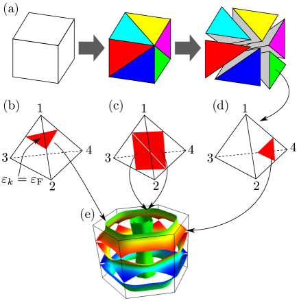
Figure 1: (a) A cell of uniform $k$-point grid is cut into six tetrahedra. Dividing a tetrahedron for (b) $\varepsilon_{1}\leq\varepsilon_{\rm F}\leq\varepsilon_{2}$, (c) $\varepsilon_{2}\leq\varepsilon_{\rm F}\leq\varepsilon_{3}$, (d) $\varepsilon_{3}\leq\varepsilon_{\rm F}\leq\varepsilon_{4}$. (e) Triangular patches are combined into Fermi surfaces.

• When $\varepsilon_{1}\leq\varepsilon_{\rm F}\leq\varepsilon_{2}\leq\varepsilon_{3}\leq\varepsilon_{4}$ [Fig. 1(b)],

  $$F =\begin{pmatrix}a_{12}&a_{21}&0&0\\ a_{13}&0&a_{31}&0\\ a_{14}&0&0&a_{41}\end{pmatrix}$$ (2)

• When $\varepsilon_{1}\leq\varepsilon_{2}\leq\varepsilon_{\rm F}\leq\varepsilon_{3}\leq\varepsilon_{4}$ [Fig. 1(c)],

  $$F =\begin{pmatrix}a_{13}&0&a_{31}&0\\ a_{14}&0&0&a_{41}\\ 0&a_{24}&0&a_{42}\end{pmatrix}$$ (3)

  $$F =\begin{pmatrix}a_{13}&0&a_{31}&0\\ 0&a_{23}&a_{32}&0\\ 0&a_{24}&0&a_{42}\end{pmatrix}$$ (4)

• When $\varepsilon_{1}\leq\varepsilon_{2}\leq\varepsilon_{3}\leq\varepsilon_{\rm F}\leq\varepsilon_{4}$ [Fig. 1(d)],

  $$F =\begin{pmatrix}a_{14}&0&0&a_{41}\\ a_{13}&a_{24}&0&a_{42}\\ a_{12}&0&a_{34}&a_{43}\end{pmatrix}$$ (5)

We compute the $k$ points and $X_{k}$ at the corner of each triangular patch as shown above then paint each patch with colors linearly interpolated from those at the corner. The normal vector for simulating the lighting conditions is obtained from the Fermi velocity computed by using the central-difference method. Finally these triangular patches are combined into Fermi surfaces [Fig. 1(e)].

2.2 French-curve interpolation

To smooth the Fermi surfaces for display, we interpolate the energy $\varepsilon_{k}$ and the $k$-dependent quantity $X_{nk}$ into a $k$ grid that is denser than that of the input. Because of band crossing, the spline, Fourier, and polynomial interpolations are not appropriate for this purpose; oscillation occurs even at points far from the band-crossing point where the energy band has a kink. Although the disentangled Wannier interpolation [19] is one of the most accurate methods to interpolate band structure, this method requires additional information (i.e. Bloch functions) and care with the parameters (energy window and projectors), so FermiSurfer has difficultly doing this interpolation automatically. Therefore, we use a simple French-curve interpolation [3], which requires only the original function itself and is robust against kinks in the band structures because of its compact formula. By using the French-curve interpolation, we obtain the interpolated function ${\tilde{f}}(x)$ in $x=[0,1]$ from the original function at four points [$f(-1)$, $f(0)$, $f(1)$, and $f(2)$] as follows:

$${\tilde{f}}(x)=a_{-1}(x)f(-1)+a_{0}(x)f(0)+a_{1}(x)f(1)+a_{2}(x)f(2),$$ (6)

where

$$a_{-1}(x) =-\frac{x(1-x)^{2}}{2},$$

$$a_{0}(x) =\left\{(1-x)^{2}+3x(1-x)+\frac{x^{2}}{2}\right\}(1-x),$$

$$a_{1}(x) =\left\{x^{2}+3(1-x)x+\frac{(1-x)^{2}}{2}\right\}x,$$

$$a_{2}(x) =-\frac{x^{2}(1-x)}{2}.$$ (7)

This interpolated function ${\tilde{f}}(x)$ satisfies ${\tilde{f}}(0)=f(0)$, ${\tilde{f}}(1)=f(1)$, ${\tilde{f}}^{\prime}(0)=\{f(1)-f(-1)\}/2$ and ${\tilde{f}}^{\prime}(1)=\{f(2)-f(0)\}/2$ and depends only on these four points. Therefore, the effect of the kink structure at the band-crossing point is confined to the vicinity of that point. We can easily extend Eq. (6) into the three dimensional case as follows:

$${\tilde{f}}(x,y,z)=\sum_{l=-1}^{2}\sum_{m=-1}^{2}\sum_{n=-1}^{2}a_{l}(x)a_{m}(y)a_{n}(z)f(l,m,n).$$ (8)

3 Installation

This section explains the procedure for installing FermiSurfer.

3.1 Executable file for Windows

The FermiSurfer package contains the source code, sample input files, documents, and the binary file bin/fermisurfer.exe for Windows. Therefore, it does not need to be built for Windows. The necessary dynamic link library files are also included.

3.2 Build by hand

For UNIX, Linux, and macOS, FermiSurfer has to be built manually. Since FermiSurfer uses the OpenGL [4] library and the OpenGL Utility Toolkit (GLUT), these libraries first have to be installed as follows:
For Debian and Ubuntu

$ sudo apt-get install freeglut3-dev

For Red Hat Enterprise Linux and CentOS

$ sudo yum install freeglut-devel.x86_64

For macOS, these libraries can be installed as part of the Xcode utility.

FermiSurfer can be built and installed by using

$ ./configure
$ make
$ make install

The binary files src/fermisurfer and src/bxsf2frmsf are then generated and copied into the directory /usr/local/bin/.

4 Input file

This section introduces the format of the FermiSurfer input file and gives examples of source code in Fortran and C to generate such a file. Also, we introduce the interface between FermiSurfer and other programs.

4.1 Input-file format

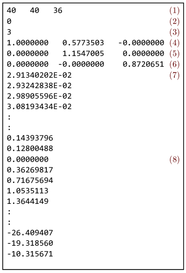
Figure 2: (Color online) Example of input file. The content labeled by line numbers in parentheses is explained in the main text. These labels do not appear in the actual input file.

To compute the Fermi surfaces with a color plot of a $k$-dependent quantity, FermiSurfer requires the number of $k$ points in three directions, the reciprocal-lattice vectors, the number of bands, the orbital energy $\varepsilon_{nk}$ where $n$ is the band index, and any $k$-dependent quantity $X_{nk}$ (e.g. the superconducting gap). The quantities $\varepsilon_{nk}$ and $X_{nk}$ are input as grid data.

Figure 2 shows an example input file called mgb2_vfz.frmsf that is contained in the FermiSurfer package. Each component of this file may be described as follows:

1. The number of $k$-grid points along each reciprocal-lattice vector;

2. Specify the type of $k$ grid (available values are 0, 1, or 2). The $k$ grid is represented as follows:

   $${\boldsymbol{k}}_{i,j,l}=x_{1i}{\boldsymbol{b}}_{1}+x_{2j}{\boldsymbol{b}}_{2}+x_{3l}{\boldsymbol{b}}_{3},$$ (9)

   where $i=1,\cdots N_{1}$, $j=1,\cdots N_{2}$, $l=1\cdots N_{3}$, and $N_{1},N_{2},N_{3}$ are the number of $k$ in the direction of each reciprocal-lattice vector. Each switch corresponds to the following $x_{\alpha i}$:

   • 0: $x_{\alpha i}=(2i-1-N_{\alpha})/(2N_{\alpha})$ (i.e., the Monkhorst-Pack grid)

   • 1: $x_{\alpha i}=(i-1)/N_{\alpha}$

   • 2: $x_{\alpha i}=(2i-1)/(2N_{\alpha})$

3. The number of bands

4. Reciprocal lattice vector 1

5. Reciprocal lattice vector 2

6. Reciprocal lattice vector 3

7. The orbital energy $\varepsilon_{nk}$. By default, FermiSurfer assumes that the Fermi energy is zero. We can shift the Fermi energy by using the menu “Shift Fermi Energy”, which is described in Sec. 5.3.

8. $k$-dependent quantity $X_{nk}$

Figures 3 and 4 show the source code in Fortran and the C, respectively, which generate this input file.

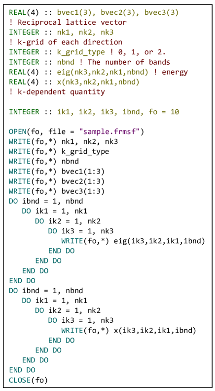
Figure 3: (Color online) Example of the Fortran source code to generate input file.

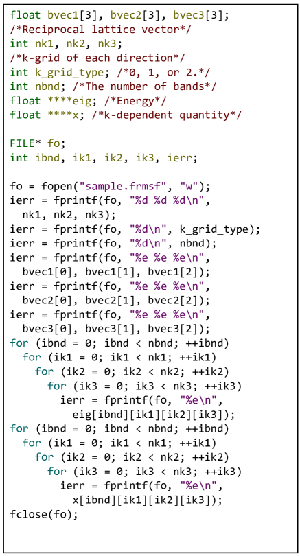
Figure 4: (Color online) Example of C source code to generate input file.

4.2 Converting BXSF files

Input files for FermiSurfer can be generated from a XCrysDen input file [13] (i.e., from the bxsf format) by using the utility program “bxsf2frmsf”, which is included in the FermiSurfer package.

4.3 Generating input file with other programs

There are two first-principles program packages, Quantum ESPRESSO [16] and Superconducting-Toolkit (SCTK) [17], that can output files compatible with FermiSurfer. Quantum ESPRESSO is a first-principles software package which bases its calculations on plane waves and pseudopotentials. Since version 6.2, this package can generate files containing the Fermi velocity and the atomic orbital character on Fermi surfaces. The Fermi velocity on the Fermi surface affects the conductivity and other properties, so knowledge of the anisotropy of this velocity is important for things such as the thermoelectric materials. Moreover, when the contributions from each atomic orbital vary on the Fermi surface, various quantities become anisotropic.

SCTK is a software package based on the density functional theory for superconductors (SCDFT) [18]. By using SCTK, we can compute the superconducting gap $\Delta_{nk}$ and the transition temperature, and generate files for displaying the superconducting gap with FermiSurfer. This is done as a postprocess after obtaining the gap function by self-consistently solving the gap equation of SCDFT. SCTK can also compute the electron-phonon renormalization and the screened Coulomb potential that can be displayed as color plots on Fermi surfaces. In Sec. 6, we show an example of study which is performed by using these programs together with FermiSurfer.

5 Usage and functions

5.1 Launch

For Linux, UNIX, or macOS, the executable file is launched as follows:

  $ fermisurfer mgb2_vfz.frmsf

A space is required between the command and the name of the input file (the sample input file mgb2_vfz.frmsf contains $z$ elements of the Fermi velocity in MgB₂).

For Windows, we launch FermiSurfer by right-clicking on the input file, choosing “Open With …”, and selecting the binary file fermisurfer.exe.

5.2 Appearance

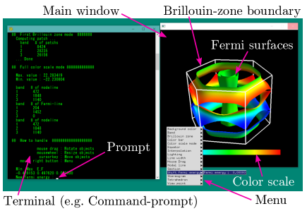
Figure 5: (Color online) Main view of FermiSurfer application.

Figure 5 shows the appearance of FermiSurfer during execution. It uses two windows (the main window and the terminal window): The main window displays the Fermi surface, the Brillouin-zone boundary, and the color scale. A pop-up menu appears upon right-clicking anywhere in the main window. It is also possible to rotate, resize, and translate the objects by dragging with the mouse, using the mouse wheel, and using the cursor keys, respectively. Information about the input data and the figure appear in the terminal window. Some commands in the pop-up menu, such as “Shift Fermi energy”, require input at the prompt in the terminal window.

5.3 Menu

We now explain the commands in the pop-up menu.

Background color

The background (Brillouin zone boundary) color is toggled between black and white (white and black).

Band

Each band can be turned on and off separately. The bands displayed are marked with an “x” in the subcommand of this command.

Brillouin zone

The type of Brillouin zone is either the first Brillouin zone or the primitive Brillouin zone (see Fig. 6). The first Brillouin zone is the region surrounded by the Bragg planes nearest to the ${\rm\Gamma}$ point, whereas the primitive Brillouin zone is a parallelepiped whose edges are the input reciprocal-lattice vectors.

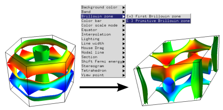
Figure 6: (Color online) The type of Brillouin zone is changed by using the “Brillouin zone” command.

Color bar

This command displays and hides the color scale.

Color scale mode

This command modifies the color scale used to display quantities on the Fermi surface. It has eight subcommands “Auto”, “Manual”, “Unicolor”, “Fermi velocity (Auto)”, “Fermi velocity (Manual)”, “Grayscale (Auto)”, and “Grayscale (Manual)”. The subcommands “Auto” and “Manual” allow the input physical quantity to be plotted in color. “Gray scale (Auto)” and “Gray scale (Manual)” plot the input physical quantity in Gray scale. The “Unicolor” subcommand paints the Fermi surface in a single color. The “Fermi velocity (Auto)” and “Fermi velocity (Manual)” subcommands produce color plots of the Fermi velocity computed internally from the energy bands. Note that “Unicolor”, “Fermi velocity (Auto)”, and “Fermi velocity (Manual)” ignore the input physical quantity. “Auto”, “Fermi velocity (Auto)”, or “Gray scale (Auto)” automatically set the blue and red extremities of the color scale to the minimum and maximum values of the displayed quantity, respectively. Conversely, subcommands “Manual”, “Fermi velocity (Manual)”, and “Gray scale (Manual)” allow the user to set the values for the blue and red extremities of the color scale.

Equator

In experiments such as ultrasonic attenuation [20] and the de Haas–van Alphen oscillation [6], the electronic states situated on lines where the Fermi velocity is orthogonal to a vector (e.g. orientation vector of the magnetic field) dominate the response; these lines are called the extremal orbits. By visualizing quantities such as electron-phonon renormalization on the extremal orbits, we can study the anisotropy appearing in these experiments. Using the “Equator” command, the user can toggle the display of the extremal orbits and modify the vector to be orthogonalized to the Fermi velocity. As an example, Fig. 7 shows the Fermi surfaces of SrVO₃ together with the extremal orbits in the (111) and (110) directions and a color plot of the Fermi velocity. This graphic shows the (110) orbit passes through the region of minimum Fermi velocity, whereas the (111) orbit does not pass through that region.

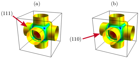
Figure 7: Fermi surfaces of SrVO₃ together with color plot of Fermi velocity. Red, green, and blue indicate the maximum, middle, and minimum Fermi velocity, respectively. Black lines on the Fermi surface indicate the extremal orbits along the (a) (111) direction and (b) (110) direction.

Interpolation

This command smooths the Fermi surface by using the French-curve interpolation (Sec. 2.1). This command modifies the number of extra points that are computed by using the interpolation.

Lighting

The Fermi surface is the interface between the electronically occupied and unoccupied regions. Via three commands, FermiSurfer allows the user to choose which side of the Fermi surface is illuminated: Both sides, the unoccupied side only, or the occupied side only. Figure 8 shows the Fermi surface of H₃S [21, 22] (Im$\bar{3}$m phase) at 150 GPa with only the occupied side illuminated. The results shows the electron pocket at the corner of the Brillouin zone and the hole pockets at the center of the Brillouin zone.

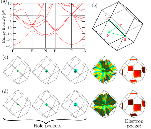
Figure 8: (a) Band structure of H₃S at 150 GPa (Im$\bar{3}$m phase) and $k$-point path for this plot (b), (c) Fermi surfaces of H₃S with both sides illuminate. The color scale gives the absolute value of the Fermi velocity. (d) Fermi surfaces of H₃S with only the occupied side illuminate. The color scale gives the absolute value of the Fermi velocity (red and blue color indicate the maximum and the minimum Fermi velocity, respectively).

Line width

This command modifies the width of the Brillouin-zone boundary, the nodal line, etc.

Mouse drag

This command changes the effect of a mouse-left-drag. The three associated subcommands “Rotate”, “Scale”, and “Translate” rotate objects along the mouse drag, resize objects with an upward or downward drag, and translate objects along the mouse drag, respectively.

Nodal line

This command toggles on and off the line on which the $k$-dependent quantity is zero (i.e., the nodal line).

Section

This command allows the user to display a two-dimensional plot of the Fermi surface from an arbitrary cross section of the Brillouin zone. This command has three subcommands: “Section”, “Modify section”, and “Modify Section (across Gamma)”. The subcommand “Section” toggles on and off the two-dimensional plot of the Fermi surface. The subcommand “Modify Section” and “Modify Section (across Gamma)” allow the user to specify the cross section. With these two subcommands, the user specifies a vector in reciprocal fractional coordinates, and the cross section is vertical to this vector. With the “Modify Section” subcommand, the cross section is perpendicular to the tip of the specified vector [Fig. 9 (a)]. Conversely, the “Modify Section (across Gamma)” subcommand puts the $\Gamma$ point in the cross section [Fig. 9 (c)]. In the latter case, the length of the specified vector is ignored.

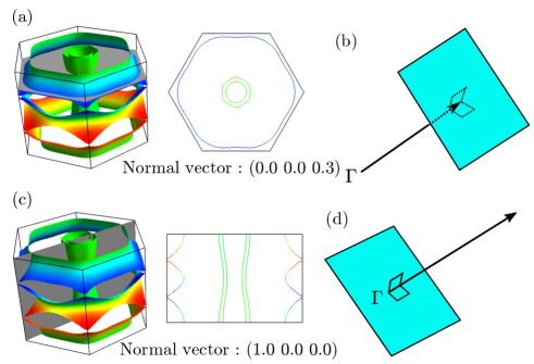
Figure 9: (Color online) (a) Fermi surface on cross section perpendicular to vector (0.0, 0.0, 0.3). (b) Schematic illustration of cross section used in panel (a). (c) Fermi surface on the cross section containing the $\Gamma$ point and perpendicular to vector (1.0, 0.0, 0.0). (d) Schematic illustration of cross section used in panel (c).

Shift Fermi energy

This command shifts the Fermi energy (which is zero by default) to an arbitrary value. This command first displays in the terminal window the current Fermi energy and the minimum and maximum energy in the input file. The user then inputs the new Fermi energy at the prompt in the terminal window, and the new Fermi surface is displayed.

Stereogram

This command toggles on and off the stereogram (parallel eye and cross eye; see Fig. 10). It contains three subcommands: “None”, “Parallel”, and “Cross”. In the default setting “None”, the stereogram is not shown. The “Parallel” and “Cross” subcommands display a parallel- and cross-eye stereogram, respectively.

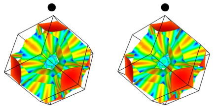
Figure 10: (Color online) Parallel-eye stereogram of Fermi surface of H₃S at 150 GPa (Im$\bar{3}$m phase) together with color plot of Fermi velocity.

Tetrahedron

This command allows the user to change the direction in which a tetrahedra is cut from a cell [Fig. 1 (a)].

Viewpoint

This command changes the viewpoint. It has three subcommands, “Scale”, “Position”, and “Rotation”, which allow the user to change the size, position, and orientation of objects, respectively. For each subcommand, the current value is first displayed, then the user is prompted to input a new value in the terminal window.

6 Examples

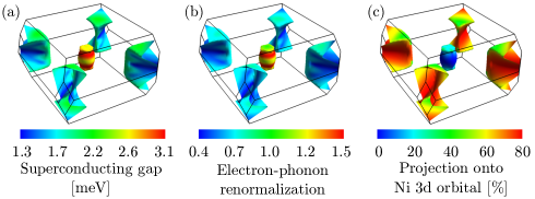
Figure 11: (Color online) Part of Fermi surface of YNi₂B₂C together with color plots of (a) superconducting gap, (b) electron-phonon renormalization, and (c) Ni 3d character.

This section discusses the use of FermiSurfer to investigate the anisotropic superconductivity in YNi₂B₂C [23, 24]. Although this material is a conventional phonon-mediated superconductor, it has highly anisotropic superconducting gaps [25, 26, 27, 28]. Figure 11(a) shows the superconducting gap computed with SCTK [17]. Small-gap (large-gap) regions appear at the corners (center) of the Brillouin zone. The same tendency appears in the color plot of the electron-phonon renormalization [Fig. 11(b)]

$$\lambda_{nk}=\sum_{q\nu n^{\prime}}\frac{2}{\omega_{q\nu}}|g_{nkn^{\prime}k+q}^{q\nu}|^{2}\delta(\varepsilon_{n^{\prime}k+q}-\varepsilon_{\rm F}),$$ (10)

where $\omega_{q\nu}$ is the phonon frequency for wave number $q$ and branch $\nu$, $\varepsilon_{nk}$ is the Kohn–Sham eigenvalue for wave number $k$ and band index $n$, $g_{nkn^{\prime}k+q}^{q\nu}$ is the electron-phonon vertex between Kohn–Sham orbitals $(n,k)$, $(n^{\prime},k+q)$ and the phonon $(\nu,q)$. Therefore, the anisotropy of the superconducting gaps comes from the anisotropy of the electron-phonon interaction. The origin of the anisotropy of the electron-phonon interaction is traced as follows: Figure 11 (c) shows the projection of the Kohn–Sham orbitals onto the Ni 3d orbitals,

$$\sum_{\tau={\rm Ni}1,{\rm Ni}2}|\langle\varphi_{nk}|\phi_{\tau,n=3,l=2,m}\rangle|^{2},$$ (11)

where $\varphi_{nk}$ is the Kohn–Sham orbital for the wave number $k$ and band index $n$, and $\phi_{\tau nlm}$ is the atomic orbital whose principal, angular momentum, and azimuthal quantum numbers are $n,l,m$, respectively. Based on this and the previous figures, we see that locations of strong Ni 3d correspond to small electron-phonon interaction, and vice versa. Further study [17] indicates that the Ni 3d state, which is localized around Ni atoms strongly screens this electron-phonon interaction. In contrast with YNi₂B₂C, MgB₂ [9] exhibits a separated multiband superconductivity [10, 11, 12], so continuous multiband superconductivity occurs in this material because of the variation of the hybridization on the Fermi surface.

7 Summary

We present herein FermiSurfer, which is a Fermi-surface viewer designed to facilitate an intuitive understanding of electronic states in metals. FermiSurfer reads the orbital energy $\varepsilon_{nk}$ and an arbitrary $k$-dependent quantity $X_{nk}$, and displays the corresponding Fermi surface color coded to indicate the value of the given quantity on the Fermi surface. Furthermore, FermiSurfer can display stereograms, nodal lines of the given quantity, cross section of the Fermi surface at any plane, and illuminate either the occupied or unoccupied side of the Fermi surface. Various first-principles software packages can generate data files readable by FermiSurfer, several examples of which are used to demonstrate the benefit of using FermiSurfer.

This work was supported by Building of Consortia for the Development of Human Resources in Science and Technology and Priority Issue (creation of new functional devices and high-performance materials to support next-generation industries) to be tackled by using Post ‘K’ Computer from the MEXT of Japan. A part of the numerical calculations in this paper were done on the supercomputer in ISSP at the University of Tokyo. The authors would like to thank Enago (www.enago.jp) for the English language review.

References

- [1] FermiSurfer Web page [online, cited http://fermisurfer.osdn.jp/].
- [2] A. Doi, A. Koide, An efficient method of triangulating equi-valued surfaces by using tetrahedral cells, IEICE TRANSACTIONS on Information and Systems 74 (1991) 214.
- [3] H. Akima, A new method of interpolation and smooth curve fitting based on local procedures, J. ACM 17 (1970) 589. doi:https://doi.org/10.1145/321607.321609.
- [4] OpenGL - The Industry Standard for High Performance Graphics [online, cited https://www.opengl.org/].
- [5] I. M. Lifshitz, M. I. Kaganov, Geometric concepts in the theory of metals, in: M. Springford (Ed.), Electrons at the Fermi Surface, Cambridge University Press, 1980, p. 4.
- [6] C. Kittel, Introduction to Solid State Physics, Wiley, 2004.
- [7] S. K. Chan, V. Heine, Spin density wave and soft phonon mode from nesting Fermi surfaces, Journal of Physics F: Metal Physics 3 (1973) 795. doi:https://doi.org/10.1088/0305-4608/3/4/022.
- [8] W. E. Pickett, Electronic structure of the high-temperature oxide superconductors, Rev. Mod. Phys. 61 (1989) 433. doi:https://doi.org/10.1103/RevModPhys.61.433.
- [9] J. Nagamatsu, N. Nakagawa, T. Muranaka, Y. Zenitani, J. Akimitsu, Superconductivity at 39 K in magnesium diboride, Nature (London) 410 (2001) 63. doi:https://doi.org/10.1038/35065039.
- [10] M. Iavarone, G. Karapetrov, A. E. Koshelev, W. K. Kwok, G. W. Crabtree, D. G. Hinks, W. N. Kang, E.-M. Choi, H. J. Kim, H.-J. Kim, S. I. Lee, Two-band superconductivity in , Phys. Rev. Lett. 89 (2002) 187002. doi:https://doi.org/10.1103/PhysRevLett.89.187002.
- [11] H. Choi, D. Roundy, H. Sun, M. Cohen, S. Louie, The origin of the anomalous superconducting properties of MgB2, Nature (London) 418 (2002) 758. doi:https://doi.org/10.1038/nature00898.
- [12] H. J. Choi, D. Roundy, H. Sun, M. L. Cohen, S. G. Louie, First-principles calculation of the superconducting transition in within the anisotropic Eliashberg formalism, Phys. Rev. B 66 (2002) 020513. doi:https://doi.org/10.1103/PhysRevB.66.020513.
- [13] A. Kokalj, Computer graphics and graphical user interfaces as tools in simulations of matter at the atomic scale, Computational Materials Science 28 (2003) 155, proceedings of the Symposium on Software Development for Process and Materials Design. doi:https://doi.org/10.1016/S0927-0256(03)00104-6.
- [14] K. Momma, F. Izumi, VESTA3 for three-dimensional visualization of crystal, volumetric and morphology data, Journal of Applied Crystallography 44 (2011) 1272. doi:{https://doi.org/10.1107/S0021889811038970}.
- [15] Winmostar [online, cited https://winmostar.com/en/].
- [16] P. Giannozzi, O. Andreussi, T. Brumme, O. Bunau, M. B. Nardelli, M. Calandra, R. Car, C. Cavazzoni, D. Ceresoli, M. Cococcioni, N. Colonna, I. Carnimeo, A. D. Corso, S. de Gironcoli, P. Delugas, R. A. D. Jr, A. Ferretti, A. Floris, G. Fratesi, G. Fugallo, R. Gebauer, U. Gerstmann, F. Giustino, T. Gorni, J. Jia, M. Kawamura, H.-Y. Ko, A. Kokalj, E. E. Küçükbenli, M. Lazzeri, M. Marsili, N. Marzari, F. Mauri, N. L. Nguyen, H.-V. Nguyen, A. O. de-la Roza, L. Paulatto, S. Poncé, D. Rocca, R. Sabatini, B. Santra, M. Schlipf, A. P. Seitsonen, A. Smogunov, I. Timrov, T. Thonhauser, P. Umari, N. Vast, X. Wu, S. Baroni, Advanced capabilities for materials modelling with Q uantum ESPRESSO, Journal of Physics: Condensed Matter 29 (2017) 465901. doi:http://doi.org/10.1088/1361-648X/aa8f79.
- [17] M. Kawamura, R. Akashi, S. Tsuneyuki, Anisotropic superconducting gaps in : A first-principles investigation, Phys. Rev. B 95 (2017) 054506. doi:https://doi.org/10.1103/PhysRevB.95.054506.
- [18] M. Lüders, M. A. L. Marques, N. N. Lathiotakis, A. Floris, G. Profeta, L. Fast, A. Continenza, S. Massidda, E. K. U. Gross, Ab initio theory of superconductivity. I. Density functional formalism and approximate functionals, Phys. Rev. B 72 (2005) 024545. doi:https://doi.org/10.1103/PhysRevB.72.024545.
- [19] I. Souza, N. Marzari, D. Vanderbilt, Maximally localized Wannier functions for entangled energy bands, Phys. Rev. B 65 (2001) 035109. doi:https://doi.org/10.1103/PhysRevB.65.035109.
- [20] J. Schrieffer, Theory Of Superconductivity, Advanced Books Classics, Avalon Publishing, 1983.
- [21] A. Drozdov, M. Eremets, I. Troyan, V. Ksenofontov, S. Shylin, Conventional superconductivity at 203 kelvin at high pressures in the sulfur hydride system, Nature 525 (2015) 73. doi:https://doi.org/10.1038/nature14964.
- [22] D. Duan, Y. Liu, F. Tian, D. Li, X. Huang, Z. Zhao, H. Yu, B. Liu, W. Tian, T. Cui, Pressure-induced metallization of dense (H 2 S) 2 H 2 with high-T c superconductivity, Scientific reports 4 (2014) 6968. doi:https://doi.org/10.1038/srep06968.
- [23] C. Mazumdar, R. Nagarajan, C. Godart, L. Gupta, M. Latroche, S. Dhar, C. Levy-Clement, B. Padalia, R. Vijayaraghavan, Superconductivity at 12 K in Y-Ni-B system, Solid State Communications 87 (1993) 413. doi:https://doi.org/10.1016/0038-1098(93)90788-O.
- [24] R. Cava, H. Takagi, H. Zandbergen, J. Krajewski, W. Peck, T. Siegrist, B. Batlogg, R. Vandover, R. Felder, K. Mizuhashi, J. Lee, H. Eisaki, S. Uchida, Superconductivity in the quaternary intermetallic compounds LnNi2B2C, Nature(London) 367 (1994) 252. doi:https://doi.org/10.1038/367252a0.
- [25] P. Martínez-Samper, H. Suderow, S. Vieira, J. Brison, N. Luchier, P. Lejay, P. Canfield, Phonon-mediated anisotropic superconductivity in the Y and Lu nickel borocarbides, Phys. Rev. B 67 (2003) 014526. doi:https://doi.org/10.1103/PhysRevB.67.014526.
- [26] T. Watanabe, M. Nohara, T. Hanaguri, H. Takagi, Anisotropy of the Superconducting Gap of the Borocarbide Superconductor with Ultrasonic Attenuation, Phys. Rev. Lett. 92 (2004) 147002. doi:https://doi.org/10.1103/PhysRevLett.92.147002.
- [27] K. Izawa, K. Kamata, Y. Nakajima, Y. Matsuda, T. Watanabe, M. Nohara, H. Takagi, P. Thalmeier, K. Maki, Gap Function with Point Nodes in Borocarbide Superconductor , Phys. Rev. Lett. 89 (2002) 137006. doi:https://doi.org/10.1103/PhysRevLett.89.137006.
- [28] T. Baba, T. Yokoya, S. Tsuda, T. Watanabe, M. Nohara, H. Takagi, T. Oguchi, S. Shin, Angle-resolved photoemission observation of the superconducting-gap minimum and its relation to the nesting vector in the phonon-mediated superconductor , Phys. Rev. B 81 (2010) 180509. doi:https://doi.org/10.1103/PhysRevB.81.180509.