Ground state phases and quantum criticalities of one-dimensional Peierls model with spin-dependent sign-alternating potentials

Abstract

We consider a one-dimensional commensurate Peierls insulator in the presence of spin-dependent sign-alternating potentials. In a continuum description, the latter supply the fermions with spin-dependent ”relativistic” masses $m_{\uparrow,\downarrow}$. The ground-state phase diagram describes three gapped phases: the CDW and SDW-like band insulator phases sandwiched by a ”mixed” phase in which the CDW and SDW superstructures coexist with a nonzero spontaneous dimerization (SD). The critical lines separating the massive phases belong to the Ising universality class. The Ising criticality is accompanied by the Kohn anomaly in the renormalized phonon spectrum. We derive a Ginzburg criterion which specifies a narrow region around the critical point where quantum fluctuations play a dominant role, rendering the adiabatic (or mean-field) approximation inapplicable.

A full account of quantum effects is achieved in the anti-adiabatic limit where the effective low-energy theory represents a massive version the N=4 Gross-Neveu model. Using Abelian bosonization we demonstrate that the description of the SD phase, including its critical boundaries, is well approximated by a sum of two effective double-frequency sine-Gordon (DSG) models subject to self-consistency conditions that couple the charge and spin sectors. Using the well-known critical properties of the DSG model we obtain the singular parts of the dimerization order parameter and staggered charge and spin susceptibilities near the Ising critical lines. We show that, in the anti-adiabatic limit, on the line $m_{\downarrow}=0$ there exists of a Berezinskii-Kosterlitz-Thouless critical point separating a Luttinger-liquid gapless phase from the spontaneously dimerized one. We also discuss topological excitations of the model carrying fractional charge and spin.

I Introduction

The effects of structural distortions or external symmetry breaking fields on the properties of strongly correlated electron systems have long been the subject of thorough investigations in condensed matter physics. A prototype model to study these effects is the one-dimensional (1D) ionic Hubbard model, which is a repulsive Hubbard chain at 1/2 filling with a staggered scalar potential. This model was originally proposed nagaosa for the description of organic mixed-stack charge-transfer crystals with alternating donor and acceptor molecules; later it has been discussed in the context of ferroelectricity in transition metal oxides egami . In view of the general interest in quantum phase transitions between gapped phases with qualitatively different symmetry properties, the main theoretical question here concerns the nature of the crossover between the Mott Insulator (MI) and Band Insulator (BI) phases, taking place when at a fixed amplitude of the staggered potential the on-site Coulomb repulsion $U$ It has been demonstrated on the basis of field-theoretical arguments FGN1 ; FGN2 that there is no direct transition between the MI and BI ground state phases. In fact, the MI-BI crossover is realized as a sequence of two continuous quantum phase transitions separated by an intermediate, fully gapped, long-range ordered phase characterized by a spontaneous dimerization (SD) (this phase is also called bond-order wave). The MI-SD transition ($U=U_{c2}$) is associated with opening of a spin gap and belongs to the Berezinskii-Kosterlitz-Thouless (BKT) universality class, whereas the SD-BI criticality ($U_{c1}$) occurs in the charge part of the spectrum and is of the quantum Ising type. In spite of some controversy in subsequent results that followed this prediction FGN1 ; FGN2 , the two-transition scenario is now well documented in both analytical and numerical works manmana ; zhang ; dyonis . The renewal of interest in the ionic Hubbard model is caused by its recent realization on optical lattices of ultracold fermionic atoms tarruell ; exp1 ; messer and the attempts to detect the predicted spontaneously dimerized phase sandwiched between the MI and BI states orignac . A SD phase has also been shown to exist in the extended 1/2-filled Hubbard model which includes a nearest-neighbor repulsion between the electrons (the UV model)nakamura ; furu .

In the 1D ionic Hubbard model defined on a rigid lattice, the region where both transitions occur is determined by the single condition that the commensurability gap of the spectrum of the MI and the one-particle gap of the BI are of the same order. As a result, the SD phase occupies a very narrow region in the phase diagram, the fact that complicates its experimental detection. However, it has been pointed out FGN1 ; zhang that inclusion of the electron-phonon interaction moves the Ising and BKT critical boundaries apart, thus removing ambiguities about the nature of the MI-BI crossover. Moreover, if the electron-phonon coupling is strong enough, the MI phase ceases to exist, and the model displays only the SD and BI phases. Thus the ionic Peierls-Hubbard model is more appropriate for a detailed study of quantum phase transitions in 1D systems controlled by a combined effect of electron-electron correlations, sign-alternating potential and electron-phonon coupling.

Spin degrees of freedom play essential role in the formation of strongly correlated phases of electrons in one dimension. Therefore, apart from the ionic staggered potential that acts on the electron charge density, the presence of a staggered magnetic field is also expected to affect the ground state phase diagram of the system. It should be pointed out that including a staggered magnetic field into consideration is not only of a theoretical interest. Experimental realizations of effective internal magnetic fields alternating over an atomic scale in certain quasi-1D compounds have already been reported in the literature dender ; aff-oshi ; ess-tsv ; zheludev . We believe that artificial manufacturing and controllable manipulation of spin-dependent potentials for ultracold atoms on optical lattices (for instance, in systems with mass-imbalanced atomic species) is a feasible task which will be performed before long. Thus it makes sense to study a more representative model of correlated fermions which incorporates staggered potentials depending on the spin projection of the particles.

As a first step in this direction, in this paper we address the role of a spin-dependent sign-alternating potential in the Peierls model Peierls which ignores the direct on-site Coulomb repulsion between the fermions ($U=0$) but accounts for those correlations between the particles which are mediated by electron-phonon coupling. In the context of the Hubbard-Peierls model, such approximation can be justified by the assumption that the phonon-mediated attraction between the electons is stronger than the Coulomb repulsion $U$ (see section III). The model is described by the Hamiltonian

$$H= - \sum_{n,\sigma}\Big{[}t_{0}+\frac{1}{2}(-1)^{n}\hat{\Delta}\Big{]}\left(c^{\dagger}_{n\sigma}c_{n+1,\sigma}+h.c.\right)$$ (1)

$$+ \sum_{n,\sigma}m_{\sigma}(-1)^{n}c^{\dagger}_{n\sigma}c_{n\sigma}+H_{\rm ph},$$

$$H_{\rm ph} = \frac{1}{2g^{2}_{0}}\int\mbox{d}x~{}\Big{[}\frac{1}{\omega^{2}_{0}}\left(\frac{\partial\hat{\Delta}}{\partial t}\right)^{2}+\hat{\Delta}^{2}\Big{]}.$$ (2)

Here $c^{\dagger}_{n\sigma}(c_{n\sigma})$ is the creation (annihilation) operator for an electron on site $n$ with spin projection $\sigma=\uparrow,\downarrow$, $t_{0}$ is the hopping matrix element, and $\hat{\Delta}$ is a real, dispersionless quantum displacement field describing phonon modes with wave vectors close to $q=\pi/a_{0}$ ($a_{0}$ being the lattice spacing). The tight-binding band of the electrons is assumed to be exactly 1/2-filled. The electron-phonon coupling is derived from the first-order modulation of the nearest-neighbor hopping amplitudes due to longitudinal lattice vibrations – the Su-Schrieffer-Heeger (SSH) model SSH ; ssh2 . $g^{2}_{0}$ is the electron-phonon coupling constant. The amplitudes of spin-dependent one-particle potentials $m_{\sigma}$ determine the scalar potential $m_{+}=(m_{\uparrow}+m_{\downarrow})/2$ which supports a site-diagonal CDW ordering, and the staggered magnetic field $m_{-}=(m_{\uparrow}-m_{\downarrow})/2$ which tends to induce a Neel (SDW) alignment of fermionic spins. In the SSH model, the phonon field $\hat{\Delta}$ couples to the electron dimerization operator

$$D_{n,n+1}=\frac{1}{2}(-1)^{n}\sum_{\sigma}\left(c^{\dagger}_{n\sigma}c_{n+1,\sigma}+h.c.\right)~{}~{}~{}$$ (3)

whose expectation value is the SD order parameter.

At $m_{\pm}=0$ and arbitrary nonzero value of $g_{0}$, the SSH model (1) has a doubly degenerate SD ground state and adequately describes structural and electronic properties of the trans-polyacetylene (CH)_x. The charge-spin separated nature of topological soliton excitations is the most celebrated feature of this model SSH ; ssh2 ; braz1 . The case of a scalar staggered potential $m_{+}\neq 0,m_{-}=0$ corresponds to a Peierls insulator with a broken charge conjugation symmetry ns ; it is relevant to the polymer cis-(CH)_x bk ; bkm .

The dimerization field (3) and the staggered electron charge or spin densities, $\rho_{s}(n)=(-1)^{n}\sum_{\sigma}c^{\dagger}_{n\sigma}c_{n\sigma}$ or $\sigma^{z}_{s}(n)=(-1)^{n}\sum_{\sigma}\sigma c^{\dagger}_{n\sigma}c_{n\sigma}$, have different parity propertis. $D_{n,n+1}$ is invariant under link parity transformation $P_{L}~{}(n\to 1-n)$ but changes its sign under site parity $P_{S}~{}(n\to-n),$ whereas for $\rho_{s}(n)$ and $\sigma^{z}_{s}(n)$ the situation is just the opposite. Therefore, starting from the spontaneously dimerized phase of a Peierls Insulator (PI) at $m_{\pm}=0$ and increasing the staggered amplitudes, one could trace a crossover to the BI regime realized as a quantum criticality. Another argument in favor of this scenario is based on the observation that the PI massive phase is an example of a topological insulator shen , whereas the BI described by the Hamiltonian (1) at $\Delta=0$ is not.

We would like to stress here that, as opposed to earlier papers furu , essler-2006 where the electron bond dimerization competing with the site-diagonal CDW potential was assumed to be explicit, everywhere in the present paper we will be dealing with spontaneous dimerization.

In the alternative, Holstein model, which is more appropriate for molecular crystals, the displacement field $\hat{\Delta}$ of the Einstein phonons couples to the staggered part of the electron charge density, $\hat{\Delta}\sum_{n\sigma}(-1)^{n}c^{\dagger}_{n\sigma}c_{n\sigma}$. In such model the role of the staggered potentials is more trivial than in the SSH model (1) because the PI phase itself and the perturbing potentials $m_{\sigma}$ are all $P_{S}$-symmetric. In this case, the staggered potentials simply lift the $\mathbb{Z}_{2}$-degeneracy of the PI state. No phase transitions are expected in this case. We thereby will not consider the Holstein model in what follows.

Throughout this paper we will be concerned with the weak-coupling limit in which all parameters of the microscopic model (1) with the dimension of energy are much less than the bandwidth $4t_{0}$:

$$|\Delta|,|m_{\sigma}|\ll W,~{}~{}~{}~{}\lambda_{0}=2g^{2}_{0}/\pi v_{F}\ll 1$$ (4)

Here $v_{F}=2t_{0}a_{0}$ is the Fermi velocity, $W\sim v_{F}/a_{0}$ is the high-energy cutoff of the electron spectrum, and $\lambda_{0}$ is the dimensionless electron-phonon coupling constant. In this case only electron states close to the right and left Fermi points are important. Being interested in the low-energy properties of the system, in the fermionic part of the Hamiltonian, Eq.(1), one can pass to the continuum limit

$${\cal H}_{f}(x)=\sum_{\sigma}\psi^{\dagger}_{\sigma}(x)\left(-\mbox{i}v_{F}\hat{\tau}_{3}\partial_{x}+\Delta\hat{\tau}_{2}+m_{\sigma}\hat{\tau}_{1}\right)\psi_{\sigma}(x)~{}~{}~{}~{}$$ (5)

Here

$$\psi_{\sigma}(x)=\left(\begin{array}[]{clcr}R_{\sigma}(x)\\ L_{\sigma}(x)\end{array}\right)$$

is a 2-spinor whose components are right and left chiral fermionic fields. The Pauli matrices $\hat{\tau}_{i}~{}(i=1,2,3)$ act in the two-dimensional Dirac-Nambu space. The quantum order parameter field ${\Delta}$ couples to the electron dimerization operator

$$D(x)=\sum_{\sigma}\psi^{\dagger}_{\sigma}(x)\hat{\tau}_{2}\psi_{\sigma}(x)$$ (6)

which is the continuum version of (3).

At $\Delta=0$ ${\cal H}_{f}$ in (5) is a sum of two Dirac models with spin dependent masses $m_{\sigma}$ accounting for external backscattering potentials. This is a BI model. At $m_{\uparrow,\downarrow}=0$ the Hamiltonian (5), with the phonon contribution (2) included, represents the continuum version of the commensurate Peierls model, introduced by Takayama, Lin-Liu and Maki tll (a field-theoretical description of an incommensurate Peierls model was developed earlier in Ref.BD ) and subsequently analyzed in great detail by Fradkin and Hirsch fh1 . A general feature of this model is dynamical generation of an exponentially small spectral gap and two-fold degeneracy of the spontaneously dimerized ground state. The study of the ground-state phase diagram of the model (1), (2) which results from the competition between the external potentials $m_{\sigma}$ and electron-phonon interaction $g^{2}_{0}$ is the main goal of the present paper.

The paper is organized as follows. In sec.2 the model is considered within a semi-classical, adiabatic approximation. We show that, as long as $m_{\uparrow},m_{\downarrow}\neq 0$, there exists a threshold for electron-phonon coupling at which an Ising transition to the spontaneously dimerized phase takes place. Taking into account quantum fluctuations within Random Phase Approximation we demonstrate the existence of a Kohn anomaly in the renormalized phonon spectrum at the critical point. We also derive a Ginzburg criterion which determines the range of applicability of the adiabatic approximation close to the transition point. In sections 3, 4 we discuss the effective low-energy model emerging in the anti-adiabatic limit, which is the case of high-frequency quantum phonons. We bosonize this model in terms of the scalar fields $\Phi_{c}$ and $\Phi_{s}$ describing collective charge and spin excitations. We identify stable minima of the potential $U(\Phi_{c},\Phi_{s})$, which incorporates all perturbations to the Gaussian models of the charge and spin sectors, and trace transformations of these minima as the parameters of the model are varied. Based on this analysis we provide a qualitative ground-state phase diagram of the model (Fig.5). We propose a well justified approximate scheme in which our bosonized model is reduced to a sum of double-frequency (DSG) models in the charge and spin sectors, coupled by self-consistency conditions. Using this picture and the known results on the DSG model we estimate the singular parts of the dimerization order parameter and the staggered charge and spin susceptibilities close to Ising criticalities. We also classify topological excitations of the model, the fractional quantum numbers they carry, and their evolution under the change of the parameters of the model. In sec.5 we consider a special case when a staggered potential is applied to one fermionic spin component only ($m_{\uparrow}\neq 0$, $m_{\downarrow}=0$). By integrating out the massive degrees of freedom we derive the effective bosonized action for the spin-$\downarrow$ fermions and discuss its properties.

The paper contains three appendices. In Appendix A we provide necessary details of Abelian bosonization used in the main text. In Appendix B we analyze stable vacua of the potential of the effective bosonized model appearing in the anti-adiabatic limit (sections 3,4). Appendix C contains technical details relating to the derivation of the effective action in sec.5.

II Adiabatic limit

II.1 Mean-field theory

In this section we adopt the adiabatic approximation in which the $\pi$-phonons are treated semiclassically. In this approach, equivalent to a mean-field theory, quantum fluctuations of the order parameter field ${\Delta}$ are neglected, so $\Delta$ becomes a classical variational parameter whose equilibrium value is found by minimizing the ground state energy of the electron-phononsystem

$$E_{0}(\Delta)=-\sum_{k,\sigma}\sqrt{k^{2}v^{2}_{F}+m_{\sigma}^{2}+\Delta^{2}}+\frac{L\Delta^{2}}{2g^{2}_{0}}$$ (7)

Simple calculations lead to

$${\cal E}(\Delta)\equiv L^{-1}\left[E(\Delta)-E(0)\right]$$

$$=\frac{\Delta^{2}}{2g_{0}^{2}}-\sum_{\sigma}\frac{{\Delta}^{2}+m^{2}_{\sigma}}{2\pi v_{F}}\left(\ln\frac{W}{\sqrt{{\Delta}^{2}+m^{2}_{\sigma}}}+\frac{1}{2}\right)$$ (8)

Minimizing (8) we obtain

$$\Delta\left(1-\frac{\lambda_{0}}{2}\sum_{\sigma}\ln\frac{2W}{\sqrt{{\Delta}^{2}+m^{2}_{\sigma}}}\right)=0$$ (9)

Re-expressing $\lambda_{0}$ in terms of the Peierls gap $\Delta_{0}$, corresponding to the unperturbed case ($m_{\uparrow}=m_{\downarrow}=0$),

$${1}/{\lambda_{0}}=\ln({2W}/{|\Delta_{0}|})$$

we find that in the region $|m_{\uparrow}m_{\downarrow}|<\Delta_{0}^{2}$ Eq.(9) leads to a doubly degenerate nonzero equilibrium solution $\pm\Delta$ satisfying

$$\Delta^{2}=-\frac{m_{\uparrow}^{2}+m^{2}_{\downarrow}}{2}+\sqrt{\frac{(m_{\uparrow}^{2}-m^{2}_{\downarrow})^{2}}{4}+\Delta_{0}^{4}},$$ (10)

whereas at $|m_{\uparrow}m_{\downarrow}|>\Delta_{0}^{2}$ only a trivial solution $\Delta=0$ remains.

Figure 1: Mean-field ground-state phase diagram. The critical lines are determined by the equation $|m_{\uparrow}m_{\downarrow}|=\Delta^{2}_{0}$.

The curves $|m_{\uparrow}m_{\downarrow}|=\Delta_{0}^{2}$ represent critical lines separating the ordered, spontaneously dimerized phase from the disordered phase representing a non-dimerized band insulator (see Fig.1). In the vicinity of these lines we can set

$$|m_{\uparrow}m_{\downarrow}|=\Delta_{0}^{2}(1+\tau),~{}~{}~{}|\tau|\ll 1$$ (11)

Then the ground state energy takes the form of a $\mathbb{Z}_{2}$-symmetric Landau expansion for a classical Ising model

$${\cal E}(\Delta) = \frac{1}{\pi v_{F}}\left(\frac{1}{2}\tau\Delta^{2}+\frac{\Delta^{4}}{4m^{2}_{*}}+\cdots\right),$$ (12)

$$\frac{1}{m^{2}_{*}} = \frac{1}{2}\sum_{\sigma}\frac{1}{m^{2}_{\sigma}}$$ (13)

In special cases $m_{\uparrow}=\pm m_{\downarrow}\equiv m$ corresponding to pure CDW or SDW external potentials the nontrivial solution reduces to $\Delta=\pm\sqrt{\Delta^{2}_{0}-m^{2}}$ and exists if $|m|<|\Delta_{0}|$. The conditions for the onset of SD in the ionic Peierls model ($m_{\uparrow}=m_{\downarrow}\neq 0$) have been discussed earlier in Refs. bk ; bkm .

In the ordered phase ($\Delta\neq 0$), the ground-state average values of the spin-symmetric and antisymmetric parts of the electron dimerization are

$$D_{+} = \sum_{\sigma}\langle D^{\sigma}_{n,n+1}\rangle\simeq\mp\frac{2\Delta}{g^{2}_{0}},$$ (14)

$$D_{-} = \sum_{\sigma}\sigma\langle D^{\sigma}_{n,n+1}\rangle\simeq\pm\frac{\Delta}{\pi v_{F}}\ln\frac{m^{2}_{\uparrow}+\Delta^{2}}{m^{2}_{\downarrow}+\Delta^{2}}$$ (15)

The average staggered parts of the electron density for a given $\sigma$ are given by

$$\rho_{\rm stag}^{\sigma} = \frac{1}{N}\sum_{n}(-1)^{n}\langle c^{\dagger}_{n\sigma}c_{n\sigma}\rangle$$ (16)

$$= -\frac{m_{\sigma}}{\pi v_{F}}\ln\frac{W}{\sqrt{m^{2}_{\sigma}+\Delta^{2}}}$$

Thus, in the presence of spin-anistropic staggered potential, the system displays two gapped phases: a non-dimerized band-insulator phase with site-diagonal charge and spin density waves and a mixed phase with a doubly degenerate ground state, in which a nonzero spontaneous dimerization coexists with the explicit CDW and SDW superstructures. As long as both $m_{\uparrow}$ and $m_{\downarrow}$ are nonzero, there exists a threshold for electron-phonon coupling, $\lambda_{c}=\ln(2W/\sqrt{|m_{\uparrow}m_{\downarrow}|})$, at which an Ising transition to the spontaneously dimerized phase ($\lambda_{0}>\lambda_{c}$) takes place. The case when one of the alternating amplitudes is zero (i.e. one fermionic spin component being massless) will be considered separately in Sec. V.

II.2 Phonon dynamics in RPA. Kohn anomaly and Ginzburg criterion

In the previous subsection we adopted the conventional mean-field approach to derive the Peierls dimerization gap in the one-particle spectrum. A consistent extention of this method to the two-particle level which allows one to include quantum fluctuations above the mean-field solution is the Random Phase Approximation (RPA) applied to the electron dynamical susceptibility and the phonon Green’s function. In doing so we will follow the seminal works by Lee, Rice and Anderson LRA and by Brazovskii and Dzyaloshinskii BD . We will show that close to the mean-field Ising transition the phonon spectrum exhibits a Kohn anomaly – softening of the phonon optical gap at $q=\pi$. Exactly at the critical point the $\pi$-phonons become gapless. We will derive a Ginzburg criterion which establishes the range of applicability of the mean-field (adiabatic) approximation in the vicinity of the transition.

Let us separate the mean-field value of the quantum field $\hat{\Delta}$ and its fluctuation (normal ordered part), $\hat{\Delta}(x,t)=\Delta+\hat{\delta}(x,t)$, $\Delta\equiv\langle\hat{\Delta}(x,t)\rangle.$ The expectation value $\Delta$ enters the mean-field fermionic Hamiltonian

$$H_{f} = \sum_{k\sigma}\psi^{\dagger}_{k\sigma}\hat{\cal H}_{k\sigma}\psi_{k\sigma},~{}~{}\psi_{k\sigma}=\left(\begin{array}[]{clcr}R_{k\sigma}\\ L_{k\sigma}\end{array}\right)$$ (20)

$$\hat{\cal H}_{k\sigma}=kv_{F}\hat{\tau}_{3}+\Delta\hat{\tau}_{2}+m_{\sigma}\hat{\tau}_{3}$$

The remaining, normal ordered part of the electron-phonon interaction

$$:H_{\rm e-ph}:~{}=\int\mbox{d}x~{}\hat{\delta}(x):\hat{D}(x):$$ (21)

accounts for quantum fluctuations of the order parameter field. Introduce the Matsubara Green’s function (GF) of the optical phonon

$${\cal G}(x,\tau)=\langle T_{\tau}:\hat{\Delta}(x,\tau)::\hat{\Delta}(0,0):\rangle$$ (22)

where $T_{\tau}$ is the imaginary-time ordering operator and averaging goes over the ground state of the system. The Fourier transform of this function,

$${\cal G}(q,\omega)=\int\mbox{d}x\int_{-\infty}^{\infty}\mbox{d}\tau~{}{\cal G}(x,\tau)~{}e^{-iqx+i\omega\tau}$$ (23)

satisfies the Dyson equation AGD

$${\cal G}^{-1}(q,\omega)={\cal G}^{-1}_{0}(\omega)-X(q,\omega)$$ (24)

where $X(q,\omega)$ is the exact dynamical dimerization susceptibility (or polarization operator) defined as the Fourier transform of the two-particle GF

$$X(x,\tau)=\langle:\hat{D}(x,\tau)::D(0,0):\rangle$$ (25)

The momentum $q$ is measured from the value $2k_{F}=\pi/a_{0}$. In Eq.(24) ${\cal G}_{0}(\omega)=g^{2}_{0}\omega^{2}_{0}/(\omega^{2}+\omega^{2}_{0})$ is the GF of the bare dispersionless optical phonon. Its spectrum gets renormalized due to quantum polarization effects of the electron subsystem incorporated in $X(q,\omega)$. In the RPA we adopt here, $X(q,\omega)$ is replaced by its value for free massive fermions described by the Hamiltonian (20):

$$X^{(0)}(q,\omega) = -\sum_{\sigma}\int\frac{\mbox{d}k}{2\pi}\int\frac{\mbox{d}\varepsilon}{2\pi}$$ (26)

$$\times {\rm Tr}~{}\{\hat{G}_{\sigma}(k+q,\varepsilon+\omega)\hat{\tau}_{2}\hat{G}_{\sigma}(k,\varepsilon)\hat{\tau}_{2}\},~{}~{}$$

where

$$\hat{G}_{\sigma}(k,\varepsilon)=-\frac{\mbox{i}\varepsilon+kv_{F}\hat{\tau}_{3}+\Delta\hat{\tau}_{2}+m_{\sigma}\hat{\tau}_{1}}{\varepsilon^{2}+k^{2}v^{2}_{F}+\Delta^{2}+m^{2}_{\sigma}},$$ (27)

is the single-fermion 2$\times$2 GF matrix.

Staying within the adiabatic approximation, we will be interested in the phonon dynamics in the low-energy limit: $|\omega|\ll|\Delta|$, $|m_{\sigma}|$. A straightforward calculation shows that in this region

$$X^{(0)}(q,\omega) = \frac{1}{\pi v_{F}}\sum_{\sigma}\Big{[}\ln\frac{2W}{\sqrt{\Delta^{2}+m^{2}_{\sigma}}}-1$$ (28)

$$~{}~{}~{}~{}~{}~{}-~{}\frac{\omega^{2}+q^{2}v^{2}_{F}-4m^{2}_{\sigma}}{4(\Delta^{2}+m^{2}_{\sigma})}\Big{]}~{}~{}~{}~{}$$

Then, in the leading order, taking into account the mean-field equation (9), we obtain

$${\cal G}_{\rm RPA}(q,\omega)=\frac{g^{2}_{0}\omega^{2}_{0}}{\omega^{2}+\Omega^{2}+q^{2}u^{2}}$$ (29)

where

$$\Omega=\Omega_{0}\zeta,~{}~{}~{}~{}u={v_{F}\Omega}/{|\Delta|},$$ (30)

Here $\Omega_{0}=\sqrt{\lambda_{0}}\omega_{0}$ is the optical gap in the standard ($m_{\sigma}=0$) adiabatic Peierls model LRA ; BD . Eq.(29) describes an optical phonon with the renormalized spectral gap $\Omega$ and group velocity $u$. The parameter

$$\zeta=\left[\frac{1}{2}\sum_{\sigma}\frac{\Delta^{2}}{\Delta^{2}+m^{2}_{\sigma}}\right]^{1/2}$$

accounts for the interplay between the order parameter $\Delta$ and staggered amplitudes $m_{\sigma}$ and varies within the interval $0<\zeta<1$. At $m_{\sigma}=0$ $\zeta=1$, and formulas (29),(30) reproduce the well-known results for the fluctuation spectrum of commensurate Peierls systems LRA ; BD . At $\Delta\ll|m_{\sigma}|$, the parameter $\zeta\sim\Delta$. In the limit $\Delta\to 0$ the velocity $u$ remains finite; however the gap $\Omega$ vanishes linearly with $\Delta$. This is a manifestation of the Kohn anomaly in the phonon spectrum signaling the onset of criticality.

Staying in the spontaneously dimerized phase, let us inspect the vicinity of the transition point more closely. In this region, using parametrization (11) with $\tau<0$ and Eq.(10), we find that $\Delta=m_{*}\sqrt{|\tau|}$. So close to the critical point $\zeta=\sqrt{|\tau|}$ the renormalized optical gap vanishes as $\Omega=\Omega_{0}\sqrt{|\tau|}.$ The consistency requirement for the adiabatic approximation assumes relative smallness of quantum fluctuations, i.e. $\langle\hat{\delta}^{2}(0,0)\rangle\ll\Delta^{2}$. Using (29) we obtain

$$\frac{\langle\hat{\delta}^{2}(0,0)\rangle}{\Delta^{2}} = \frac{1}{\Delta^{2}}\int\frac{\mbox{d}q}{2\pi}\int\frac{\mbox{d}\omega}{2\pi}~{}{\cal G}_{RPA}(q,\omega)$$ (31)

$$= \frac{\sqrt{\lambda_{0}}\omega_{0}}{2\Delta\zeta}\ln\left(\frac{2W}{\sqrt{\lambda_{0}}\omega_{0}\zeta}\right)$$

Deep in the ordered phase, i.e. at $\Delta_{0}\gg|m_{\uparrow}m_{\downarrow}|$, when $\Delta\sim\Delta_{0}$, the parameter $\zeta\sim 1$ and (31) reduces to the standard estimate of the ratio $\langle\delta^{2}\rangle/\Delta^{2}$ for a conventional PI. In this case the condition of the applicability of the adiabatic approximation reads $(\Omega_{0}/\Delta_{0})\ln(2W/\Omega_{0})\ll 1$. The situation changes in the vicinity of the phase transition. At $\tau\to 0$

$$\frac{\langle\hat{\delta}^{2}\rangle}{\Delta^{2}}\sim\frac{\Omega_{0}}{m_{*}}\frac{\ln(1/|\tau|)}{|\tau|}$$ (32)

Since $|\tau|\ll 1$, the ratio (32) can be small only in the region

$$1\gg|\tau|\gg{\rm Gi}$$ (33)

where (with the logarithmic accuracy)

$${\rm Gi}\sim\frac{\Omega_{0}}{m_{*}}\ln\frac{m_{*}}{\Omega_{0}}$$ (34)

is the Ginzburg parameter. The inequality (33) only makes sense if ${\rm Gi}\ll 1$, i.e. $\Omega_{0}\ll m_{*}$. If the latter condition is satisfied, (33) represents the Ginzburg criterion for our problem which specifies the range of applicability of the semiclassical adiabatic (or mean-field) approximation near the critical point (see e.g.cardy ). However, inside the narrow region $|\tau|\ll{\rm Gi}\ll 1$ the order parameter field cannot be be treated classically, and quantum fluctuations dominate the dynamics of the system.

Thus one arrives at the important conclusion: while away from criticality the adiabatic approximation is valid as long as $\Omega_{0}\ll|\Delta|,|m_{\sigma}|$, the immediate vicinity of the critical point ($|\tau|\ll{\rm Gi}$) remains beyond the reach of the above semiclassical approach. An adequate route to correctly account for strong quantum fluctuations of the order parameter is the anti-adiabatic approximation which is discussed in detail in the remainder of this paper. In particular, we will show that the classical Ising transition as it is seen from the ”adiabatic distance” (33), transforms to a quantum criticality belonging to the quantum Ising universality class when quantum fluctuations become dominant.

II.3 Topological solitons

We conclude this section by commenting on the fermion quantum numbers of solitons of the field $\Delta(x)$, that is the coordinate dependent solutions that interpolate between the two degenerate vacua $\pm{\Delta}_{*}$ of the potential (8) in the spontaneously dimerized phase:

$$\lim_{x\to\infty}\Delta(x)=\pm{\Delta}_{*},~{}~{}~{}~{}\lim_{x\to-\infty}\Delta(x)=\mp{\Delta}_{*}$$

At $m_{\uparrow}=m_{\downarrow}=0$ the Hamiltonian (5) anticommutes with $\hat{\tau}_{1}$ and, hence, displays a conjugation symmetry $\psi\to\hat{\tau}_{1}\psi$ which takes positive-energy solutions of the Dirac equation into negative-energy ones. As a consequence, in the presence of solitonic background, there exist normalizable, self-conjugate zero-energy solutions of the Dirac equation carrying fractional quantized fermion numbers $q=\pm 1/2$. This was established almost simultaneously in quantum field theory jr and condensed matter physics SSH ; ssh2 ; braz1 . The mass term of the Dirac Hamiltonian breaks the charge conjugation symmetry. As a result, for spinless fermions, the fermion number $q$ is no longer half-integer but depends on the parameters of the Hamiltonian gw ; ns :

$$q=1/2-(1/\pi)\tan^{-1}({m}/{\Delta}_{*}),$$

$m$ being the Dirac mass. Since the Hamiltonian is additive in spin indices, one can use the above result for each fermionic spin component because for both of them the topological background field $\Delta(x)$ is the same. Then one obtains the charge and spin quantum numbers for the topological solitons of the model (1):

$$Q = 1-\frac{1}{\pi}\left[\tan^{-1}\left(\frac{m_{\uparrow}}{\Delta_{*}}\right)+\tan^{-1}\left(\frac{m_{\downarrow}}{\Delta_{*}}\right)\right]$$ (35)

$$S^{z} = -\frac{1}{2\pi}\left[\tan^{-1}\left(\frac{m_{\uparrow}}{\Delta_{*}}\right)-\tan^{-1}\left(\frac{m_{\downarrow}}{\Delta_{*}}\right)\right]$$ (36)

For arbitrary nonzero values of the staggered amplitudes, such that $|m_{\uparrow}|\neq|m_{\downarrow}|$, topological excitations in our model carry both charge and spin which continuously depend on the ratios $m_{\uparrow,\downarrow}/{\Delta}_{*}$. The cases $m_{\uparrow}=\pm m_{\downarrow}$ are special. The former case describes an ionic spin-symmetric PI in which the staggered potential affects only the electron charge density. In such system the solitons carry a nonzero fractional charge, $Q\neq 0$, but are spinless, $S^{z}=0$. The latter case corresponds to a staggered magnetic field affecting only the spin density of the electrons. Accordingly, the solitons carry a nonzero spin, $S^{z}\neq 0$, but are neutral, $Q=0$.

The quantized charge-spin separated quantum numbers of the soliton excitations of the Peierls model SSH ; ssh2 ; braz1 are recovered only in the limit $m_{\uparrow,\downarrow}\to 0$. In this limit, the spin-dependent Dirac masses serve as regulators, and the result ($Q=\pm 1,S^{z}=0$ or $Q=0,S^{z}=\pm 1/2$) depends of the relative sign of the vanishing amplitudes $m_{\uparrow}$ and $m_{\rm\downarrow}$.

III Antiadiabatic limit, quantum phonons. Bozonized Hamiltonian

We now turn to the field-theoretical description of the Peierls model in the the anti-adiabatic limit, in which the phonons are characterized by high frequency, $\omega_{0}\gg|\Delta|,|m_{\sigma}|$. This regime was first considered by Fradkin and Hirsch fh1 . By integrating the phonons out, they derived a purely fermionic effective low-energy action which has the form of a nonchiral N=2 Gross-Neveu (GN) model GN ; witten1 ; shankarwitten ; DHN ; zamo2 with a local four-fermion interaction mediated by the phonons. The staggered potentials appearing in (1) supply the fermions with spin dependent $\gamma^{5}$-masses. The resulting fermionic model is described by the Lagrangian ${\cal L}={\cal L}_{\rm GN}+{\cal L}_{\rm ext}$, where

$${\cal L}_{\rm GN} = \mbox{i}\bar{\psi}_{\alpha}\gamma^{\mu}\partial_{\mu}\psi_{\alpha}+\frac{1}{2}g^{2}_{0}\left(\bar{\psi}_{\alpha}\psi_{\alpha}\right)^{2}$$ (37)

$${\cal L}_{\rm ext} = -\mbox{i}\bar{\psi}_{\alpha}\gamma^{5}\left(m_{+}\delta_{\alpha\beta}+m_{-}\sigma^{3}_{\alpha\beta}\right)\psi_{\beta}$$ (38)

Here $\alpha,\beta$ are the spin indices, $\bar{\psi}=\psi^{\dagger}\gamma^{0}$, and for the Dirac $\gamma$-matrices the following representation is chosen: $\gamma^{0}=\hat{\tau}_{2}$, $\gamma^{1}=\mbox{i}\hat{\tau}_{1}$, $\gamma^{5}=\gamma^{0}\gamma^{1}=\hat{\tau}_{3}$.

III.1 Bosonization of O(4) Gross-Neveu model

For future purposes, using the bosonization method (see e.g. gnt ), we first recapitulate the main findings of Ref.fh1 that follow from the well-known properties of the massless GN model (37). By decoupling each complex fermion into a pair of real fields, one recasts the model (37) as an O(4)-invariant theory of four interacting Majorana fermions

$${\cal H}_{\rm GN}=-\frac{\mbox{i}v_{F}}{2}~{}\xi^{a}\hat{\tau}_{3}\partial_{x}\xi^{a}+\frac{1}{2}g^{2}_{0}\left(\xi^{a}_{R}\cdot\xi^{a}_{L}\right)^{2}$$ (39)

where $\xi^{a}=(\xi^{a})^{\dagger}~{}(a=1,2,3,4)$. Using the bosonization approach, one transforms ${\cal H}_{\rm GN}$ to a direct sum of two weakly perturbed SU(2)₁ Wess-Zumino-Novikov-Witten (WZNW) models (see Appendix A)

$${\cal H}_{\rm GN}={\cal H}_{c}+{\cal H}_{s},~{}~{}~{}{\cal H}_{c,s}={\cal H}^{(c,s)}_{\rm WZNW}+g^{2}_{0}{\bf J}^{c,s}_{R}\cdot{\bf J}^{c,s}_{L},~{}~{}~{}$$ (40)

where ${\bf J}^{c,s}_{R,L}$ are chiral vector currents of the corresponding critical WZNW model (93). The charge-spin separated structure of the Hamiltonian (40) reflects the symmetry group equivalence O(4) $\approx$ SU(2) $\otimes$ SU(2). The theory (40) can be reformulated as a sum of two identical quantum sine-Gordon models for bosonic fields $\Phi_{c}$ and $\Phi_{s}$ (see Eq.(92)):

$${\cal H}(x) = \sum_{a=c,s}{\cal H}_{a}(x),$$ (41)

$${\cal H}_{a}(x) = \frac{v}{2}\left\{\left(1-\frac{g^{2}_{0}}{2\pi v}\right)\Pi^{2}_{a}(x)+\left(1+\frac{g^{2}_{0}}{2\pi v}\right)\left(\partial_{x}\Phi_{a}(x)\right)^{2}\right\}$$ (42)

$$~{}~{}-\frac{g^{2}_{0}}{2(\pi\alpha)^{2}}\cos\sqrt{8\pi}\Phi_{a}(x).~{}~{}~{}~{}$$

All irrelevant corrections to Eq.(42) with the Gaussian scaling dimension 4 and higher are neglected (see however sec.V). In terms of the original fermionic fields $\psi_{\alpha}$, the cosine terms in (42) represent marginally relevant backscattering (spin sector) and Umklapp processes (charge sector). On the Kosterlitz-Thouless phase diagram k , each of the sine-Gordon Hamiltonians flows (in the RG sense) along the SU(2)-symmetric separatrix towards the strong-coupling infrared stable fixed point.

The main feature of the ground state of the GN model (39) is a spontaneous breakdown of the discrete $\gamma^{5}$-symmetry (with the continuous SO(4)-symmetry kept unbroken) and double degeneracy of the ground state. The sum of the Majorana mass bilinears, $\mbox{i}\sum_{a}\xi^{a}_{R}\xi^{a}_{L}\sim\sum_{\alpha}\bar{\psi}_{\alpha}\psi_{\alpha}$, acquires a nonzero vacuum expectation value witten1 ; shankarwitten . The dynamically generated mass

$$m_{c}=m_{s}\equiv{\mathfrak{m}}\simeq\Lambda\exp\left(-\pi v_{/}g^{2}_{0}\right),~{}~{}~{}\Lambda\sim v_{F}/\alpha$$ (43)

coincides with the single-soliton mass of the $\beta^{2}=8\pi$ SG model. In terms of the original complex fermions the symmetry breaking order parameter is just the electron dimerization operator (3) which in the continuum limit has the following bosonic representation (see Appendix A)

$$D~{}\sim\langle{\rm Tr}~{}\bar{\psi}\psi\rangle~{}\sim~{}\cos\sqrt{2\pi}\Phi_{c}\cos\sqrt{2\pi}\Phi_{s}$$ (44)

In the ground state, the fields $\Phi_{c}$ and $\Phi_{s}$ are locked at one of the degenerate minima of the cosine potential in (42)

$$\left(\Phi_{c}\right)_{j_{c}}=\sqrt{\frac{\pi}{2}}~{}j_{c},~{}~{}~{}~{}\left(\Phi_{s}\right)_{j_{s}}=\sqrt{\frac{\pi}{2}}~{}j_{s},$$

$$(j_{c},~{}j_{s}=0,\pm 1,\pm 2,\ldots)$$ (45)

The lattice of the PI vacua (III.1) is shown in Fig. 2(a). Accordingly

$$\langle D\rangle_{j_{c},j_{s}}=D_{0}(-1)^{j_{c}+j_{s}},$$ (46)

where (since the Gaussian scaling dimension of the dimerization operator is $d=1$)

$$D_{0}=|\langle\cos\sqrt{2\pi}\Phi_{c}\rangle\langle\cos\sqrt{2\pi}\Phi_{s}\rangle|=C^{2}{\mathfrak{m}}/\Lambda$$ (47)

where $C$ is a numerical constant calculated in Ref.LZ1 . Eq.(46) demonstrates double degeneracy of the SD ground state: depending on the parity of the sum $j_{c}+j_{s}$, $\langle D\rangle$ takes values $\pm D_{0}$.

The spontaneously dimerized phase of the GN model is a typical example of a strongly correlated state. Contrary to the adiabatic model, a single-fermionic branch of the spectrum of the model (41), (42) is absent. The only elementary excitations are topological quantum solitons of the $\beta^{2}=8\pi$ sine-Gordon model (42), either in the charge or spin sector. They correspond to vacuum-vacuum transitions with $\Delta\Phi_{c,s}=\pm\sqrt{\pi/2}$. These are the transitions between nearest-neighbor sites of the PI vacuum lattice, Fig. 2(a). According to the definitions (86) given in Appendix A, the charge and spin carried by the solitons are defined as

$$Q = \sqrt{\frac{2}{\pi}}\int_{-\infty}^{\infty}\mbox{d}x~{}\partial_{x}\Phi_{c}(x)=\sqrt{\frac{2}{\pi}}\Delta\Phi_{c},$$

$$S^{z} = \frac{1}{\sqrt{2\pi}}\int_{-\infty}^{\infty}\mbox{d}x~{}\partial_{x}\Phi_{s}=\frac{1}{\sqrt{2\pi}}\Delta\Phi_{s}$$ (48)

and hence are equal to $Q=\pm 1$ and $~{}S^{z}=\pm 1/2$, respectively. Thus, the physical picture of a charge-spin separated solitonic spectrum of a commensurate Peierls insulator emerging in the anti-adiabatic limit is qualitatively the same as in the adiabatic model fh1 . In both limits spontaneous dimerization of the system emerges at arbitrarily small electron-phonon coupling. The SU(2) $\times$ SU(2) representation (41), (42) of the O(4) GN model proves efficient: the characterization of the spectrum in terms of the charge-spin separated quantum solitons is in full agreement with the exact result zamo2 ; witten1 that the spectrum of the O(4) GN model only consists of kinks.

III.2 Bosonized form of staggered potentials and Band Insulator vacua

Under the action of staggered one-particle potentials and in the absence of electron-phonon coupling ($g_{0}=0$) the system represents a band insulator with gapped single-particle excitations carrying both the charge and spin quantum numbers. On the other hand, in a PI state single-particle excitations are absent and the whole spectrum is exhausted by collective charge and spin modes described in terms of quantum solitons. To understand the interplay between the phonon induced electron-electron correlations that tend to dimerize the system and sign-alternating potentials that support a BI regime, it is instrumental to have a representation of the staggered potentials in terms of scalar fields $\Phi_{c,s}=(\Phi_{\uparrow}\pm\Phi_{\downarrow})/\sqrt{2}$ describing collective charge and spin modes. Using formulas (A) and (89) of Appendix A, we have

$$\Delta H_{\rm stag} = \sum_{n\sigma}m_{\sigma}(-1)^{n}c^{\dagger}_{n\sigma}c_{n\sigma}\to\int\mbox{d}x~{}{\cal H}_{\rm stag}(x);$$

$${\cal H}_{\rm stag}= - \frac{1}{\pi\alpha}\left(m_{\uparrow}\sin\sqrt{4\pi}\Phi_{\uparrow}+m_{\downarrow}\sin\sqrt{4\pi}\Phi_{\downarrow}\right)$$

$$= - \left(\frac{2m_{+}}{\pi\alpha}\right)\sin\sqrt{2\pi}\Phi_{c}\cos\sqrt{2\pi}\Phi_{s}$$ (49)

$$- \left(\frac{2m_{-}}{\pi\alpha}\right)\cos\sqrt{2\pi}\Phi_{c}\sin\sqrt{2\pi}\Phi_{s}.$$

(we remind that $m_{\pm}=(m_{\uparrow}\pm m_{\downarrow})/2$). We see that, on one hand, the BI Hamiltonian splits into spin-$\uparrow$ and spin-$\downarrow$ independent components, each of them representing the quantum sine-Gordon model for the field $\Phi_{\sigma}$ with the coupling constant $\beta^{2}=4\pi$ (free fermion point). Not surprisingly, no such decomposition is possible in terms of the charge and spin fields $\Phi_{c}$ and $\Phi_{s}$. The vacua of the BI phase are shown in Fig.2(b).

Figure 2: Sets of vacua in PI and BI phases. Notations: $\varphi_{c,s}=\sqrt{2\pi}\Phi_{c,s}$. (a) Lattice of PI vacua. (b) BI vacua, black and open circles correspond to the cases $m_{+}>m_{-}$ and $m_{+}<m_{-}$, respectively.

Without loss of generality everywhere below we will assume that $m_{\pm}>0$. Then from (49) one determines the vacuum values of the fields $\Phi_{c}$ and $\Phi_{s}$:

$$\left(\Phi\right)^{(c)}_{\rm vac}=\sqrt{\frac{\pi}{8}}+\sqrt{\frac{\pi}{2}}n_{c},~{}~{}\left(\Phi\right)^{(s)}_{\rm vac}=\sqrt{\frac{\pi}{2}}n_{s}$$ (50)

at $m_{+}>m_{-}$, and

$$\left(\Phi\right)^{(c)}_{\rm vac}=\sqrt{\frac{\pi}{2}}n_{c},~{}~{}\left(\Phi\right)^{(s)}_{\rm vac}=\sqrt{\frac{\pi}{8}}+\sqrt{\frac{\pi}{2}}n_{s},$$ (51)

at $m_{+}<m_{-}$, with the restriction that the integers $n_{c}$ and $n_{s}$ have the same parity: $n_{c}+n_{s}=0,\pm 2,\pm 4,\ldots$. In such description, fundamental (single-particle) excitations in the noninteracting BI are interpreted as topological excitations of the model (49) associated with the transitions between nearest-neighbor degenerate vacua (50) or (50). These are the transitions with $|\Delta n_{c}|=|\Delta n_{s}|=1$ which yield the charge $Q=\pm 1$ and spin $S^{z}=\pm 1/2$.

IV Anti-adiabatic Peierls model with staggered, spin-dependent potentials

Having overviewed the structure of the vacuum and elementary excitations for the ”pure” PI ($m_{\pm}=0$) and BI ($g_{0}=0$) phases, here we consider the general case with all perturbations to the Gaussian part of the Hamiltonian present. The total bosonized Hamiltonian reads:

$${\cal H}(x) = {\cal H}^{(0)}_{c}+{\cal H}^{(0)}_{s}+U(\Phi_{c},~{}\Phi_{s});$$ (52)

$$U(\Phi_{c},~{}\Phi_{s})= - \frac{g^{2}_{0}}{2(\pi\alpha)^{2}}\left(\cos\sqrt{8\pi}\Phi_{c}+\cos\sqrt{8\pi}\Phi_{s}\right)$$ (53)

$$- \left(\frac{2m_{+}}{\pi\alpha}\right)\sin\sqrt{2\pi}\Phi_{c}\cos\sqrt{2\pi}\Phi_{s}$$

$$- \left(\frac{2m_{-}}{\pi\alpha}\right)\cos\sqrt{2\pi}\Phi_{c}\sin\sqrt{2\pi}\Phi_{s},$$

where ${\cal H}^{(0)}_{c,s}$ are the Hamiltonians of free massless bosons in the charge and spin sectors, given by the first line in Eq.(42). In this section we will study in detail the interplay between the competing marginally relevant GN two-cosine perturbation and strongly relevant staggered potentials and describe the outcome of this competition.

IV.1 Classical vacua

Stable vacua of the potential $U(\Phi_{c},\Phi_{s})$ in Eq.(53) identify massive ground-state phases of the model. A straightforward analysis done in Appendix B reveals the following properties of the potential. In the regions $|m^{2}_{+}-m^{2}_{-}|>\left(g^{2}_{0}/\pi\alpha\right)^{2}$ the degenerate vacua of $U(\Phi_{c},~{}\Phi_{s})$ form a square lattice with periods $\sqrt{\pi/2}$, Fig.2(b). These vacua are not affected by the electron-phonon interaction and coincide with those of the ”pure” band insulator, Eqs. (50),(51). This is the non-dimerized BI phase of the model.

At $|m^{2}_{+}-m^{2}_{-}|<\left(g^{2}_{0}/\pi\alpha\right)^{2}$ the profile of the potential changes. At $m_{\pm}=0$ the SD massive phase has a different set of vacua, Eqs.(III.1), Fig.2(a). As schematically shown in Fig.3, upon increasing the difference $|m^{2}_{+}-m^{2}_{-}|$, symmetrically located pairs of new minima appear and start moving from their neighboring initial PI values towards the nearest BI value. Depending on the ratio $m_{+}/m_{-}$, the trajectories in the $(\Phi_{c},\Phi_{c})$ plane along which the minima of the potential $U$ move split in two groups. The line $\Phi_{c}=\Phi_{s}$ is a separatrix which sets apart the CDW-dominated sector ($m_{+}>m_{-}$) and the SDW-dominated sector ($m_{+}<m_{-}$). In the CDW sector the vacuum values of the charge field move from $\Phi_{c}=0$ and $\sqrt{\pi/2}$ towards the BI value $\Phi_{c}=\sqrt{\pi/8}$ where the two minima merge. The spin field $\Phi_{s}$ stays equal zero at both initial and final points of the trajectory and satisfies the condition $\Phi_{s}<\Phi_{c}$ in between (see Fig.3). The picture in the SDW sector is similar and is obtained from the former case by interchanging $m_{+}\leftrightarrow m_{-}$, $\Phi_{c}\leftrightarrow\Phi_{s}$.

Figure 3: Evolution of the minima of the potential $U(\varphi_{c},\varphi_{s})$ (shown by the asterisks) in the spontaneously dimerized phase $|m^{2}_{+}-m^{2}_{-}|<(g^{2}_{0}/\pi v_{F})$ upon increasing $m_{\pm}$. Notations: $\varphi_{c,s}=\sqrt{2\pi}\Phi_{c,s}$.

Thus, the equations

$$m^{2}_{+}-m^{2}_{-}=\pm\left(\frac{g^{2}_{0}}{\pi\alpha}\right)^{2}$$ (54)

determine classical critical lines separating phases with and without spontaneous dimerization. We will see below that quantum fluctuations significantly modify the equations for the critical curves.

Let us consider the region $|m^{2}_{+}-m^{2}_{-}|<\left(g^{2}_{0}/(\pi\alpha)\right)^{2}$ and inspect the shape of the potential in the vicinity of the critical lines (54). Below we will specialize to the case $m_{+}>m_{-}$. It is convenient to use the $(\Phi_{\uparrow},\Phi_{\downarrow})$ representation of the potential and pass to dimensionless quantities. The details can be found in Appendix B. The potential takes the form (see Eq.(94)):

$${\cal{U}}(x,y) \equiv \left(\frac{\pi\alpha}{g_{0}}\right)^{2}U(\Phi_{\uparrow},\Phi_{\downarrow})~{}~{}~{}$$ (55)

$$= -\cos x\cos y-a\sin x-b\sin y~{}~{}$$

Let us expand ${\cal{U}}(x,y)$ in the vicinity of the point $(x,y)=(\pi/2,\pi/2)$ which is a minimum of ${\cal{U}}$ in the BI phase. For small deviations from this point, $q_{1}=x-\pi/2$, $q_{2}=y-\pi/2$, to the accuracy $O(q^{6})$, we have

$${\cal{U}}(q_{1},q_{2}) = {\cal{U}}(0,0)+\left[\frac{1}{2}\left(aq^{2}_{1}+bq^{2}_{2}\right)-q_{1}q_{2}\right]$$ (56)

$$+ \left[\frac{1}{6}(q^{2}_{1}+q^{2}_{2})q_{1}q_{2}-\frac{1}{24}\left(aq^{4}_{1}+bq^{4}_{2}\right)\right]$$

The quadratic part of ${\cal{U}}$ is diagonalized by an appropriate SO(2) rotation of the vector ${\bf q}=(q_{1},q_{2})$: $\delta{\cal{U}}^{(2)}=\frac{1}{2}\left(\lambda_{1}\eta^{2}_{1}+\lambda_{2}\eta^{2}_{2}\right)$, where $\eta_{1}$ and $\eta_{2}$ are normal coordinates, and

$$\lambda_{1,2}=f_{+}\pm\sqrt{f^{2}_{-}+1},~{}~{}~{}f_{\pm}=(a\pm b)/2=m_{\pm}\pi\alpha/g^{2}_{0}.$$

In the vicinity of the transition point we can use the parametrization $f_{+}=\left(1+\tau/2\right)\cosh\gamma$, $f_{-}=\left(1+\tau/2\right)\sinh\gamma$, so that $f^{2}_{+}-f^{2}_{-}=1+\tau$, where $\gamma>0$ and $|\tau|\ll 1$ such that $\tau>0$ ($\tau<0$) for the BI (PI) phase. So

$$\lambda_{1}=2\cosh\gamma+O(\tau),~{}~{}~{}~{}\lambda_{2}=\frac{\tau}{2\cosh\gamma}$$ (57)

From (57) it follows that the point $(x,y)=(\pi/2,\pi/2)$ is a minimum of the potential at $\tau>0$ (BI phase) and a saddle point at $\tau<0$ (SD phase). The rigidities of the potential around this point in the $\eta_{1}$ and $\eta_{2}$ directions are drastically different: $\eta_{2}$ is a soft direction where the stiffness $\lambda_{2}\sim\tau$ is small, whereas in the orthogonal direction $\eta_{1}$ the stiffness is much larger, $\lambda_{1}\geq 2$. So, in the vicinity of the point $(\pi/2,\pi/2)$, at small deviations from the criticality ($|\tau|\ll 1$) the potential has the shape of a narrow channel along the $\eta_{2}$-direction. For this reason, in the low-energy limit, it is sufficient to consider the effective potential ${\cal{U}}(\eta_{1},\eta_{2})$ only along the ”easy” direction $\eta_{2}$. The resulting expansion of the potential

$${\cal{U}}(\eta_{1},\eta_{2}) \to {\cal{U}}(0,\eta_{2})~{}~{}~{}~{}~{}$$ (58)

$$= {\rm const}~{}+~{}\frac{\tau}{4\cosh\alpha}~{}\eta^{2}_{2}~{}+~{}\frac{1}{8\cosh\alpha}~{}\eta^{4}_{2}~{}~{}~{}$$

reveals its effectively one-dimensional double-well structure which unambiguously indicates the existence of an Ising transition at $\tau=0$.

IV.2 Quantum approach

IV.2.1 Perturbative estimations

Having identified stable vacua of the potential $U(\Phi_{c},\Phi_{s})$, now we turn to a quantum description of the PI-to-BI crossover. According to (III.1), in the unperturbed PI phase ($m_{\pm}=0$) the vacuum values of the fields $\Phi_{c}$ and $\Phi_{s}$ are multiples of $\sqrt{\pi/2}$, so that the averages

$$|\langle\cos\sqrt{2\pi}\Phi_{c,s}(0)\rangle_{0}|=C_{0}({\mathfrak{m}}/\Lambda)^{1/2}\neq 0$$ (59)

(the numerical value of the prefactor $C_{0}$ is calculated in Ref.LZ1 ). Consider the regime $m_{\pm}\ll{\mathfrak{m}}$, in which the staggered fields can be treated as small perturbations. Apparently, perturbative expansions of $\langle\cos\sqrt{2\pi}\Phi_{a}(0)\rangle~{}(a=1,2)$ contain only even powers of the staggered amplitudes $m_{\pm}$:

$$\langle\cos\sqrt{2\pi}\Phi_{c,s}(0)\rangle$$

$$=C_{0}\left({\mathfrak{m}}/{\Lambda}\right)^{1/2}\left[1-C\left({m_{\pm}}/{\mathfrak{m}}\right)^{2}+\cdots\right]$$ (60)

Here $C\sim 1$ is a positive numerical constant. We observe that perturbation theory breaks down at $m_{\pm}\sim{\mathfrak{m}}$, which is roughly the conditions for the Ising criticalities.

IV.2.2 Reduction to coupled double-frequency sine-Gordon models

In the pure PI phase the operators $\cos\sqrt{2\pi}\Phi_{c,s}$ have nonzero expectation values, whereas $\sin\sqrt{2\pi}\Phi_{c,s}$ are short-ranged fluctuating fields with zero averages. Therefore, in the leading order, the staggered potentials in (53) can be replaced by

$${\cal H}_{\rm stag}\to-\left(\frac{2\bar{m}_{+}}{\pi\alpha}\right)\sin\sqrt{2\pi}\Phi_{c}-\left(\frac{2\bar{m}_{-}}{\pi\alpha}\right)\sin\sqrt{2\pi}\Phi_{s}~{}~{}~{}~{}~{}~{}$$ (61)

with

$$\bar{m}_{+}=m_{+}\langle\cos\sqrt{2\pi}\Phi_{s}\rangle,~{}~{}~{}~{}\bar{m}_{-}=m_{-}\langle\cos\sqrt{2\pi}\Phi_{c}\rangle$$ (62)

As a result, the effective Hamiltonian decouples into two quantum double-frequency sine-Gordon (DSG) models

$${\cal H}_{\rm eff}=\sum_{a=c,s}{\cal H}^{(a)}_{\rm DSG},$$ (63)

$${\cal H}^{(a)}_{\rm DSG}={\cal H}^{(a)}_{0}-\eta_{a}\cos\sqrt{8\pi}\Phi_{a}-\zeta_{a}\sin\sqrt{2\pi}\Phi_{a}$$ (64)

$$\eta_{c}=\eta_{s}=\frac{g^{2}_{0}}{2(\pi\alpha)^{2}},~{}~{}\zeta_{c}=\frac{2\bar{m}_{+}}{\pi\alpha},~{}~{}\zeta_{s}=\frac{2\bar{m}_{-}}{\pi\alpha}~{}~{}~{}~{}$$ (65)

The DSG model has been analyzed in detail in Refs. [DM, ,FGN2, ]. It describes an interplay between two relevant perturbations to the Gaussian conformal field theory ${\cal H}^{(a)}_{0}$ with the ratio of their scaling dimensions equal to 4. Because the two perturbations have different parity symmetries and, consequently, the field configurations which minimize one perturbation do not minimize the other, the competition between them produces an Ising quantum critical point DM .

The additive structure of the Hamiltonian (63) might lead to a wrong conclusion that the effective model has a charge-spin separated form and hence should display two independent quantum Ising transitions, one in each sector. In fact, in agreement with the above classical analysis, at a given ratio $m_{+}/m_{-}\neq 1$, there exists only one transition. At the quantum level, the key point is the self-consistency conditions (62) that couple the charge and spin sectors. We will argue now that, in the CDW-like case ($m_{+}>m_{-}$) the Ising transition is described by ${\cal H}^{(c)}_{\rm DSG}$, whereas the criticality in ${\cal H}^{(s)}_{\rm DSG}$ is avoided. In the SDW-like case ($m_{+}<m_{-}$) the situation is just the opposite.

The critical point in the DSG model (64) can be estimated by comparing the mass gaps that would open up if the two perturbations were acting alone. The $\eta_{a}$-term generates the Peierls mass gap ${\mathfrak{m}}$, Eq.(43). The mass gap generated by the $\zeta_{a}$-term scales as $m_{\zeta_{a}}\sim\Lambda\left(\zeta_{a}\alpha/\Lambda\right)^{2/3}.$ So the critical values of the effective staggered amplitudes, $\bar{m}_{\pm}^{*}$, should coincide and be of the order of

$$\bar{m}_{+}^{*}=\bar{m}_{-}^{*}\sim\Lambda\left({\mathfrak{m}}/\Lambda\right)^{3/2}$$ (66)

Exponential smallness of the r.h.s. of (66) shows that quantum fluctuations significantly reduce the critical value of the staggered amplitudes as compared to the classical estimate (54).

If for any bare values of $m_{\pm}$ the transitions in the charge and spin DSG models (64) had occurred independently, then Eqs.(66) and (62) would imply that $m_{+}/m_{-}={\langle\cos\sqrt{2\pi}\Phi_{c}\rangle}/{\langle\cos\sqrt{2\pi}\Phi_{s}\rangle}.$ However, already the perturbative expansions (60) show that the above relation cannot be valid except for the special case $m_{+}=m_{-}$ (see below). Therefore, at a given ratio $m_{+}/m_{-}\neq 1$, there can be only one Ising transition: either in the charge DSG model if $m_{+}>m_{-}$, or in the spin DSG model if $m_{+}<m_{-}$.

It has been shown in Ref.[FGN2, ] that mapping of the DSG model (64) onto a generalized 1D quantum Ashkin-Teller model makes the Ising criticality accessible by non-perturbative means. The lowest-energy sector of the theory is described by a single critical quantum Ising model, i.e. a CFT with central charge $c=1/2$. Using this correspondence, one can find the low-energy projections of the physical fields near the transition. In particular, it has been shown FGN2 that $\cos\sqrt{2\pi}\Phi_{a}\sim\mu$, $\sin\sqrt{2\pi}\Phi_{a}\sim I+\varepsilon$, where $\mu$ and $\varepsilon$ are the disorder field and energy density of the critical Ising model cft , $I$ being the identity operator. Accordingly, the average values of these operators are

$$\langle\cos\sqrt{2\pi}\Phi_{a}\rangle_{\zeta_{a}}\sim\left[\frac{(\zeta_{a}^{*}-\zeta_{a}}{\zeta_{a}^{*}}\right]^{1/8},~{}~{}\zeta_{a}<\zeta_{a}^{*}$$

$$~{}~{}~{}~{}~{}~{}~{}~{}~{}~{}~{}~{}~{}~{}~{}~{}~{}~{}=~{}~{}~{}~{}0,~{}~{}~{}~{}~{}~{}~{}~{}~{}~{}~{}~{}~{}~{}~{}~{}~{}\zeta_{a}>\zeta_{a}^{*}$$ (67)

$$\langle\sin\sqrt{2\pi}\Phi_{a}\rangle_{\zeta_{a}}-\langle\sin\sqrt{2\pi}\Phi_{c}\rangle_{\zeta_{a}^{*}}$$

$$~{}~{}~{}~{}~{}~{}~{}~{}~{}~{}~{}~{}~{}~{}~{}~{}~{}~{}~{}~{}\sim~{}\frac{\zeta_{a}-\zeta_{a}^{*}}{\zeta_{a}^{*}}\ln\frac{\zeta_{a}^{*}}{|\zeta_{a}-\zeta_{a}^{*}|}$$ (68)

So, as follows from (67), at $m_{+}>m_{-}$, in the vicinity of the Ising transition the effective staggered magnetic field $\bar{m}_{-}$ vanishes as $m_{+}\to m^{*}_{+}$, so that the condition ${\bar{m}_{-}}\sim\Lambda({\mathfrak{m}}/\Lambda)^{3/2}$ cannot be satisfied. On approaching the critical point the spin degrees of freedom remain gapped since the DSG Hamiltonian ${\cal H}^{(s)}_{\rm DSG}$ effectively transforms to a SG model. The Ising critical point in the charge DSG model ${\cal H}^{(c)}_{\rm DSG}$ separates the mixed massive phase in with coexisting site-diagonal CDW and SD ($m_{+}<m^{*}+$) from the pure CDW phase where dimerization vanishes ($m_{+}>m^{*}_{+}$).

Close to the transition the dimerization order parameter (44) is proportional to $\langle\cos\sqrt{2\pi}\Phi_{c}\rangle$ and, according to (67), vanishes as

$$\langle D\rangle\sim\Theta(m^{*}_{+}-m_{+})\left(m^{*}_{+}-m_{+}\right)^{1/8}$$ (69)

as $m_{+}\to m_{+}^{*}$. The singular part of the staggered charge
density $\langle\rho_{\rm stag}\rangle$ is proportional to the average $\langle\sin\sqrt{2\pi}\Phi_{c}\rangle$. As follows from (68), it remains continuous across the transition, but its derivative which determines the staggered compressibility of the system, displays a logarithmic singularity:

$$\kappa_{\rm stag}=\partial\langle\rho_{\rm stag}\rangle/\partial m_{+}\sim-\ln|m_{+}-m^{*}_{+}|$$ (70)

Since the staggered potentials break the SU(2)$\times$ SU(2) symmetry of the GN model, on lowering the energy scale in the charge sector the parameters of the Hamiltonian ${\cal H}_{\rm DSG}^{(c)}$, $\zeta_{c}$ and $\eta_{c}$, will undergo renormalization. Moreover, the compactification radius of the field $\Phi_{c}$ (i.e. the Luttinger liquid parameter $K_{c}$ whose unperturbed value is $K^{(0)}_{c}=\beta^{2}/8\pi=1$) will also acquire a (nonuniversal) dependence on $m^{2}_{\pm}$. However, up to $O(m^{2}_{-})$ corrections, the condition $\bar{m}^{*}_{+}\sim\Lambda({\mathfrak{m}}/\Lambda)^{3/2}$ implies that in the region $m_{+}>m_{-}$ the Ising transition occurs at $m_{+}=m^{*}_{+}\sim{\mathfrak{m}}.$ In the SDW-like case, $m_{+}<m_{-}$, the situation is identical to the above scenario with the charge and spin DSG models interchanged. Here the renormalized scalar amplitude $\bar{m}^{*}_{+}$ vanishes at the Ising criticality, and the critical point is determined by the condition $m_{-}=m^{*}_{-}\sim{\mathfrak{m}}.$ Formula (69) still holds with the replacement of $m_{+}$ by $m_{-}$, and the logarithmic singularity at the transition becomes the property of the staggered spin susceptibility of the system:

$$\chi_{\rm stag}=\partial\langle{s}^{z}_{\rm stag}\rangle/\partial m_{-}\sim-\ln|m_{-}-m^{*}_{-}|$$ (71)

A special situation arises when $m_{+}=\pm m_{-}$. This is the case when the staggered potential acts only on fermions with a certain spin projection. This case will be considered in sec.V. Here we only mention that this is the situation when the two DSG models ${\cal H}^{(c)}_{\rm DSG}$ and ${\cal H}^{(s)}_{\rm DSG}$ become identical, implying that the Ising criticality will be reached simultaneously in both sectors. However, the universality class of the critical point will change. The effective low-energy theory will be described in terms of two copies of identical critical quantum Ising models, or equivalently two species of massless Majorana fermions. Since two Majorana fermions can be combined into a single Dirac (i.e. complex) fermion, the original discrete $\mathbb{Z}_{2}\times\mathbb{Z}_{2}$ symmetry gets enlarged to the continuous $U(1)$.

IV.3 Topological excitations with fractional quantum numbers

For the SD (mixed) phase realized at $|m^{2}_{+}-m^{2}_{-}|^{2}<(g^{2}_{0}/\pi\alpha)^{2}$, the set of degenerate vacua of the potential $U(\Phi_{c},\Phi_{s})$ is discussed in detail in Appendix B. In accordance with the double degeneracy of the SD ground state, there exist two sets of minima $\mbox{\boldmath$\varphi$}=(\varphi_{c},\varphi_{s})$ [see Eqs. (99)]:

$$\mbox{\boldmath$\varphi$}^{(1)}_{>}=[\varphi_{+}+\pi n_{c},~{}\varphi_{-}+\pi n_{s}],$$

$$\mbox{\boldmath$\varphi$}^{(2)}_{>}=[-\varphi_{+}+\pi(n_{c}+1),~{}-\varphi_{-}+\pi n_{s}]$$ (72)

at $m_{+}>m_{-}$, and

$$\mbox{\boldmath$\varphi$}^{(1)}_{<}=[\varphi_{-}+\pi n_{c},~{}\varphi_{+}+\pi n_{s}],$$

$$\mbox{\boldmath$\varphi$}^{(2)}_{<}=[-\varphi_{-}+\pi n_{c},~{}-\varphi_{+}+\pi(n_{s}+1)]$$ (73)

at $m_{+}<m_{-}$. In the above formulas $\varphi_{c,s}=\sqrt{2\pi}\Phi_{c,s}$, $\varphi_{\pm}=(x_{0}\pm y_{0})/2$, where $x_{0}$ and $y_{0}$ are given by the expressions (99). The parameters $\varphi_{\pm}$ vary within the interval $(0,\pi/2)$, and the sum of integers $n_{c}$ and $n_{s}$ is constrained to be an even number.

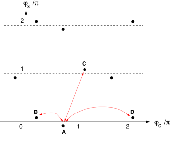
Figure 4: The set of degenerate vacua of the potential $U(\Phi_{c},\Phi_{s})$ in the mixed SD phase at $m_{+}>m_{-}$. The coordinates of the points A,B,C,D are $A=(\pi-\varphi_{+},-\varphi_{-})$, $B=(\varphi_{+},~{}\varphi_{-})$, $C=(\pi+\varphi_{+},~{}\pi-\varphi_{-})$, $D^{(1)}=(2\pi+\varphi_{+},~{}\varphi_{-})$.

The location of the vacua in the CDW-like phase ($m_{+}>m_{-}$) is shown Fig.4. Stable topological excitations represent dimerization kinks which correspond to $\mbox{\boldmath$\varphi$}^{(1)}\leftrightarrow\mbox{\boldmath$\varphi$}^{(2)}$ transitions between nearest vacua. These are of the AB, AC and AD types. The charge $Q$ and spin $S^{z}$ of these excitations, determined by formulas (48), take fractional (non-quantized) values because at any nonzero $m_{+}\neq m_{-}$ the SU(2) $\times$ SU(2) symmetry of the pure PI phase is explicitly broken. The double-well periodic structure of the potential, typical for the DSG model DM , implies the existence of ”short” (AB) and ”long” (AD) kinks carrying the quantum numbers

$$Q_{\mp}=1\mp\frac{2\varphi_{+}}{\pi},~{}~{}~{}S^{z}=\mp\frac{\varphi_{-}}{\pi}$$ (74)

In the limit $\varphi_{\pm}\to 0$ both kinks convert to a spinless soliton of the pure PI model: $Q_{\pm}\to 1$, $S^{z}\to 0$. On approaching the SD-BI transition point ($\varphi_{+}\to\pi/2$, $\varphi_{-}\to 0$) the AD and AB kinks transform to spin-singlet states ($S^{z}_{\pm}=0$) either of two particles (holes), $Q_{+}=2$, or a particle-hole state, $Q_{-}=0$. The AD transition describes an excitation with the spin $S^{z}=1/2$ and the charge $Q={2\varphi_{+}}/{\pi}$, interpolating between a neutral spin-1/2 soliton of the PI and a quasiparticle of the BI. The AD and AC excitations stay massive across the Ising transition. However, at criticality, the short kink AB loses its charge and mass and transforms to a collective gapless excitonic mode (c.f. Ref.FGN1 ).

Comparing (72) and (73) one finds out that the quantum numbers of topological excitations in the SDW-like phase ($m_{+}<m_{-}$) can be deduced from the previous case by using the interchange symmetry $\varphi_{+}\leftrightarrow\varphi_{-}$, $Q\leftrightarrow 2S^{z}$. The analog of the short and long kinks (74) is

$$Q=\pm\frac{2\varphi_{+}}{\pi},~{}~{}~{}S^{z}=\frac{1}{2}\mp\frac{\varphi_{-}}{\pi}$$ (75)

These kinks interpolate between a neutral spin-1/2 soliton of the pure PI model at $\varphi_{\pm}\to 0$ and particle-hole states with the total spin $S=0$ or $1$ at the transition point ($\varphi_{+}\to 0$, $\varphi_{-}\to\pi/2$). There is also an excitation with the charge $Q=1$ and fractional spin $S^{z}={\varphi_{-}}/{\pi}$ which interpolates between a spinless soliton carrying a unit of charge in the pure PI phase and a quasiparticle of the BI insulator. As in the CDW-like phase, here too we find that at the criticality there exists a neutral collective mode that loses its mass and has zero spin.

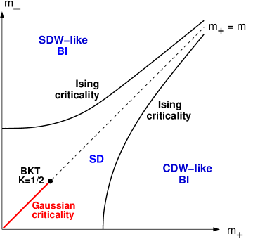
Figure 5: Phase diagram of the model in the anti-adiabatic limit..

V Peierls model in the vicinity of the line ${\bf m_{+}=m_{-}}$

In this section we consider the situation when the amplitudes of the staggered potentials $m_{\uparrow,\downarrow}$ are strongly different, e.g. $m_{\uparrow}\gg m_{\downarrow}.$ As before, it will be still assumed that $0<m_{\uparrow,\downarrow}\ll\Lambda$. The above condition includes the case when the sign-alternating potential is applied to one spin component only, e.g.

$$m_{\downarrow}=0,~{}~{}~{}m_{+}=m_{-}$$ (76)

Let us first consider the case (76) in the adiabatic limit. A nontrivial solution for the order parameter,

$$\Delta^{2}=-\frac{m_{\uparrow}}{2}+\sqrt{\frac{m^{2}_{\uparrow}}{4}+\Delta^{4}_{0}},$$ (77)

indicates the onset of spontaneous dimerization at arbitrarily small electron-phonon coupling $\lambda_{0}$ for any nonzero $m_{\uparrow}$. This fact is entirely due to the existence of a gapless fermionic component (with $\sigma=\uparrow$) and the adiabatic approximation we adopted here. As follows from (77), when the electron-phonon interaction is strong enough, $m_{\uparrow}\ll\Delta_{0}$, the massiveness of the spin-$\uparrow$ fermions is unimportant, and, in the leading order, $\Delta$ is given by the standard expression for a canonical (massless) Peierls model, $\Delta\simeq\Delta_{0}$. For a weak electron-phonon coupling, $m_{\uparrow}\gg\Delta_{0}$, $\Delta$ vanishes at $\Delta_{0}\to 0$ according to the quadratic law $\Delta\simeq\Delta^{2}_{0}/m_{\uparrow}$.

Now we turn to the anti-adiabatic limit of quantum phonons and consider the case $m_{\uparrow}\gg m_{\downarrow}$. Starting from the massive GN model with spin-dependent Dirac masses

$${\cal H} = \sum_{\sigma}\psi^{\dagger}_{\sigma}\left(-\mbox{i}v_{F}\hat{\tau}_{3}\partial_{x}+m_{\sigma}\hat{\tau}_{1}\right)\psi_{\sigma}$$ (78)

$$~{}~{}-~{}\frac{1}{2}g^{2}_{0}\left(\sum_{\sigma}\psi^{\dagger}_{\sigma}\hat{\tau}_{2}\psi_{\sigma}\right)^{2}$$

we will integrate the heavy spin-$\uparrow$ electrons out and derive an effective Hamiltonian describing the low-energy degrees of freedom for the light $\sigma=\downarrow$ electrons.

Apart from the usual Umklapp processes $R^{\dagger}_{\uparrow}R^{\dagger}_{\downarrow}L_{\downarrow}L_{\uparrow}+h.c.\sim\cos\sqrt{8\pi}\Phi_{c}$ involving electrons with opposite spin projections, the interaction in (78) also includes Umklapp scattering of the electrons with the same spin projection:

$$\sum_{\sigma}\left[R^{\dagger}_{\sigma}(x)R^{\dagger}_{\sigma}(x+\alpha)L_{\sigma}(x+\alpha)L_{\sigma}(x)+h.c.\right]$$

$$~{}~{}~{}~{}~{}~{}~{}~{}~{}~{}~{}~{}~{}~{}~{}~{}~{}~{}~{}~{}~{}~{}~{}~{}\sim~{}\sum_{\sigma}\cos\sqrt{16\pi}\Phi_{\sigma}(x)$$ (79)

At the Gaussian ultraviolet fixed point such perturbation has scaling dimension 4 and hence is strongly irrelevant. However, the staggered potentials break the SU(2)$\times$SU(2) symmetry of the GN model and cause renormalization of the compactification radii of the scalar fields. If this renormalization is strong enough, the Umklapp processes (79) may become relevant and thus affect the phase diagram of the system. Such situation is known to exist in a 1D half-filled tight-binding model of spinless fermions with a strong enough nearest-neighbor repulsion (by the Jordan-Wigner correspondence, this is equivalent to a XXZ spin-1/2 chain with exchange anisotropy parameter $J_{z}/J_{x}>1$) giam .

We will assume that $m_{\uparrow}$ is large enough to suppress the Umklapp and forward scattering processes in the spin-$\uparrow$ component. So the ”heavy” subsystem can be treated in terms of free massive fermions with the mass $m_{\uparrow}$. The unperturbed Euclidian action for the spin-$\downarrow$ electrons has the form of a DSG model

$$S^{(0)}_{\downarrow}=\int\mbox{d}^{2}{\bf r}~{}\Big{\{}\frac{1}{2}\left(1+\frac{g^{2}_{0}}{4\pi v_{F}}\right)\left(\mbox{\boldmath$\nabla$}\Phi_{\downarrow}({\bf r})\right)^{2}$$

$$-\frac{m_{\downarrow}}{\pi\alpha v_{F}}\sin\sqrt{4\pi}\Phi_{\downarrow}({\bf r})-\frac{g^{2}_{0}}{(2\pi\alpha)^{2}v_{F}}\cos\sqrt{16\pi}\Phi_{\downarrow}({\bf r})\Big{\}}~{}~{}~{}$$ (80)

where ${\bf r}=(v_{F}\tau,x)$ is a 2D Euclidian coordinate. For a weak electron-phonon coupling, the last term in (80) remains strongly irrelevant, with the scaling dimension $d=4\left(1-g^{2}_{0}/4\pi v_{F}+\cdots\right),$ still close to 4. In such case (80) reduces to the $\beta^{2}=4\pi K$ SG model describing massive spinless fermions with a weak short-distance repulsion (massive Thirring model gnt ). As shown in Appendix C, interaction between the ”light” (spin-$\downarrow$) and ”heavy” (spin-$\uparrow$) fermions leads to a significant renormalization of the parameters of the effective action $S_{\downarrow}$. The second-order correction $\Delta S_{\downarrow}$ to the ”bare” action $S^{(0)}_{\downarrow}$ is given by formula (108). Adding it to (80) and rescaling the field, $\Phi_{\downarrow}\to\sqrt{K}\Phi_{\downarrow}$ we arrive at the effective action

$$S^{({\rm eff})}_{\downarrow}=S^{(0)}_{\downarrow}+\Delta S^{({\rm eff})}_{\downarrow}=\int\mbox{d}^{2}{\bf x}~{}\Big{\{}\frac{1}{2}(\mbox{\boldmath$\nabla$}\Phi_{\downarrow})^{2}$$

$$-\frac{\eta}{\alpha^{2}}\sin\sqrt{4\pi K}\Phi_{\downarrow}-\frac{\zeta}{(2\pi\alpha)^{2}}\cos\sqrt{16\pi K}\Phi_{\downarrow}\Big{\}}$$ (81)

where

$$\eta=\frac{m_{\downarrow}\alpha}{\pi v_{F}},~{}~{}~{}~{}\zeta=\frac{g^{2}_{0}}{v_{F}}+C_{1}\left(\frac{g^{2}_{0}}{v_{F}}\right)^{2}\left(\frac{\Lambda}{m_{\uparrow}}\right)^{2}$$ (82)

are dimensionless amplitudes and

$$\frac{1}{K}=1+\frac{g^{2}_{0}}{4\pi v_{F}}+\frac{1}{2}\left(\frac{g^{2}_{0}}{\pi v_{F}}\right)^{2}\ln\frac{\Lambda}{m_{\uparrow}}$$ (83)

We see that renormalization effects arising in the second order in $(g_{0}^{2})$ due to the coupling between the electrons with opposite spins enhance the values of the parameters $K^{-1}$ and $\zeta$.

Let us first consider the case $m_{\downarrow}=0~{}(\eta=0)$. The action (81) is a SG model at $\beta^{2}=16\pi K$ and represents a bosonized version of the massless N=1 GN model fh1 . Even though the dependence of the parameters $K$ and $\zeta$ on the bare coupling constants and the mass $m_{\uparrow}$ are nonuniversal, Eq.(83) suggests that in the region $(g^{2}_{0}/v_{F})^{2}\ln(\Lambda/m_{\uparrow})\sim 1$ a critical value of $K=K_{c}=1/2$ should be reached, below which the Umklapp term in (81) is relevant and supports spontaneous dimerization of the spin-$\downarrow$ electron subsystem. Thus, at $K>1/2$ the cosine perturbation is strongly irrelevant, and the spin-$\downarrow$ fermionic subsystem is in a Luttinger-liquid gapless phase gnt ; giam with critical exponents continuously varying with $K$. The line of Gaussian fixed points terminates at $K_{c}=1/2$ (see Fig.5). At this point the system undergoes a BKT transition to a spinless massive Peierls phase. The critical value of the ”heavy” component mass $m_{\uparrow}$ when the Peierls transition occurs is extremely small

$$m_{\uparrow}\simeq\Lambda\exp\left[-\frac{1}{2}\left(\frac{2\pi v_{F}}{g^{2}_{0}}\right)^{2}\right]$$ (84)

We see that, in the case when a staggered field is applied only to one spin component, the picture emerging in the adiabatic approach differs from that emerging in the anti-adiabatic limit: in the former case the onset of SD occurs at arbitrarily small electron-phonon coupling, whereas in the latter case there exists a BKT transition from the metallic phase to the PI phase of spin-$\downarrow$ fermions.

When the amplitude $m_{\downarrow}$ is finite but still much less than $m_{\uparrow}$, the effective action (81) contains the $\eta$-term which supports a BI phase. The negative sign of the Umklapp amplitude ensures that at any nonzero $m_{\downarrow}$ there should exist an Ising criticality at some critical value of $m_{\downarrow}=m^{(\rm crit)}_{\downarrow}(g_{0}^{2},m_{\uparrow})$ separating the SD and BI massive phases.

Fig.5 summarizes the main qualitative features of the anti-adiabatic model.

VI Conclusions

In this paper, we have studied the ground-state properties of the one-dimensional Peierls model at 1/2-filling SSH ; ssh2 subjected to a simultaneous action of staggered scalar potential ($m_{+}$) and a sign-alternating magnetic field ($m_{-}$). Our goal was to describe the interplay between the electron-phonon interaction which, when acting alone, would lead to the onset of a spontaneously dimerized Peierls phase with a charge-spin separated low-energy spectrum, and external, spin-dependent, staggered single-particle potentials that transform a one-dimensional metal to a standard band insulator with CDW and SDW superstructures and the usual quasiparticle excitations, carrying both the charge and spin. The electron-phonon interaction has been treated using both the semiclassical, adiabatic approximation and in the anti-adiabatic limit in which the high-frequency quantum phonons generate an effective attraction between the electrons. We specialized to the weak coupling regime in which the low-energy degrees of freedom are adequately described by the continuum electron-phonon model tll with spin-dependent Dirac masses $m_{\uparrow,\downarrow}=(m_{+}\pm m_{-})/2$.

The phase diagram of the model is depicted in Fig.5. Depending on the sign of the parameter $F=|m^{2}_{+}-m^{2}_{-}|>(g^{2}_{0}/\pi\alpha)^{2}$, where $g_{0}$ and $\alpha$ are the electron-phonon coupling constant and short-distance cutoff parameter, respectively, the system occurs in one of three gapped phases: a CDW dominated band insulator phase realized at $F>0$, $m_{+}>m_{-}$, a SDW dominated band insulator at $F>0$, $m_{+}<m_{-}$, and a mixed Peierls phase at $F<0$, in which the CDW and SDW superstructures coexist with a nonzero spontaneous dimerization. The massive phases are separated by critical lines ($F=0$) belonging to the universality class of the quantum Ising model. Except for the symmetry line $m_{+}=m_{-}$, quantum effects do not change the phase diagram qualitatively, i.e. only affect the location of the critical lines.

The semiclassical treatment of the phonon degrees of freedom shows that at $m_{\pm}\neq 0$ spontaneous dimerization of the system occurs at a finite critical value of the dimensionless electron-phonon coupling constant, $\lambda_{c}\equiv\left(2g^{2}_{0}/\pi v_{F}\right)_{c}=\ln(2W/\sqrt{|m_{\uparrow}m_{\downarrow}|})$, $W$ being of the order of the electron bandwidth. The onset of the Ising criticality is accompanied by the Kohn anomaly in the renormalized phonon spectrum. We have demonstrated that the adiabatic approximation cannot provide a satisfactory description of the model in the vicinity of the Ising criticality. We have derived a Ginzburg criterion which determines a narrow region around the critical point, where quantum fluctuations play a dominant role and the adiabatic (or mean-field) approximation is no longer applicable.

The line $m_{+}=m_{-}$ is a special case of an external staggered potential applied to one fermionic spin component only. In the adiabatic approximation, along this line the system is unstable against a spontaneous dimerization at arbitrarily small electron-phonon coupling. We show that, contrary to such conclusion, the analysis carried out in the anti-adiabatic limit, indicates the existence of a Berezinskii-Kosterlitz-Thouless critical point which separates a Luttinger-liquid gapless phase from the spontaneously dimerized one (see Fig.5).

In the anti-adiabatic limit, where the quantum $\pi$-phonons are characterized by a high frequency $\omega_{0}\gg\Delta_{0}/\sqrt{\lambda_{0}}$ ($\Delta_{0}$ being the electron spectral gap of the Peierls insulator), the effective low-energy model represents a massive version of the non-chiral N=2 Gross-Neveu model which, apart from the conventional four-fermion interaction induced by the phonons fh1 , also includes spin-dependent fermionic $\gamma^{5}$-mass terms. We bosonized this model in terms of two scalar fields, $\Phi_{c}$ and $\Phi_{s}$, describing the collective charge and spin degrees of freedom. The resulting continuous model is given by Eq.(52) and represents a charge-spin separated sum of two $\beta^{2}=8\pi$ sine-Gordon models coupled by strongly relevant $m_{\pm}$-perturbations. For all $m_{+}\neq m_{-}$ the phase diagram of Fig.5 was derived from the analysis of stable vacua of the potential (53). We have shown that the description of the spontaneously dimerized (SD) phase, including its boundaries with the band insulator (BI) phases, can be well approximated by a sum of two effective double-frequency sine-Gordon (DSG) models subject to self-consistency conditions that couple the charge and spin sectors. We have argued that, in the region $m_{+}>m_{-}$ the quantum Ising transition to the CDW-like BI phase is described by the ”charge” DSG model, whereas the criticality in ”spin” DSG model is avoided. At $m_{+}<m_{-}$ the situation is just the opposite. Using the well-studied critical properties of the DSG model DM ,FGN1 ,FGN2 we found the critical exponent 1/8 characterizing the power-law decay of the dimerization order parameter near the Ising criticality. We have also shown that the staggered compressibility of the system near the SD-CDW transition, as well as the staggered spin susceptibility at the SD-SDW transition display logarithmic singularities.

We have also discussed the topological excitations of the model and derived the fractional values the charge $Q$ and $z$-projection of the spin $S^{z}$ they carry. We have traced the evolution of the topological kinks when moving from the SD phase to one of the BI phases.

The results obtained in this paper also apply to the Peierls-Hubbard model which includes a Coulomb onsite repulsion between the electron under the condition that the latter is small compared to the attraction induced by the electron-phonon coupling. A detailed description of the Peierls-Hubbard chain perturbed by a spin-dependent staggered potential is the subject of future studies.

Appendix A Some details of Abelian bosonization

Here we provide a brief account of the Abelian bosonization rules used in the main text of the paper. For more details we refer to Ref. [gnt, ].

The model of free massless fermions with spin-1/2

$${\cal H}^{(0)}_{f}(x)=-\mbox{i}v\sum_{\sigma=\uparrow,\downarrow}\psi^{\dagger}_{\sigma}(x)\tau_{3}\partial_{x}\psi_{\sigma}(x),~{}~{}\psi_{\sigma}(x)=\left(\begin{array}[]{clcr}R_{\sigma}(x)\\ L_{\sigma}(x)\end{array}\right)$$

is equivalent to a theory of two massless bosons:

$${\cal H}^{(0)}_{b} = \frac{v}{2}\sum_{\sigma=\uparrow,\downarrow}\left[\Pi^{2}_{\sigma}(x)+\left(\partial_{x}\Phi_{\sigma}(x)\right)^{2}\right]$$ (85)

$$= \frac{v}{2}\sum_{a=c,s}\left[\Pi^{2}_{a}(x)+\left(\partial_{x}\Phi_{a}(x)\right)^{2}\right]$$

where the charge and spin scalar fields ($\Phi_{c},\Phi_{s}$) and their conjugate momenta ($\Pi_{c},\Pi_{s}$) are defined as

$$\Phi_{c,s}=\frac{\Phi_{\uparrow}\pm\Phi_{\downarrow}}{\sqrt{2}},~{}~{}~{}\Pi_{c,s}=\frac{\Pi_{\uparrow}\pm\Pi_{\downarrow}}{\sqrt{2}}$$

The smooth parts of the fermionic charge and spin densities are given by

$$\rho(x)=\sqrt{\frac{2}{\pi}}\partial_{x}\Phi_{c}(x),~{}~{}~{}~{}~{}S^{z}(x)=\frac{1}{\sqrt{2\pi}}\partial_{x}\Phi_{c}$$ (86)

Using the correspondence

$$R^{\dagger}_{\sigma}L_{\sigma}\to-({\mbox{i}}/{2\pi\alpha})e^{-i\sqrt{4\pi}\Phi_{\sigma}},~{}~{}~{}L^{\dagger}_{\sigma}R_{\sigma}\to({\mbox{i}}/{2\pi\alpha})e^{i\sqrt{4\pi}\Phi_{\sigma}}$$

one finds bosonized expressions for the dimerization operator

$$D(x) = \sum_{\sigma}\bar{\psi}_{\sigma}\psi_{\sigma}=\sum_{\sigma}\psi^{\dagger}_{\sigma}(x)\hat{\tau}_{2}\psi_{\sigma}(x)$$ (87)

$$= -\frac{1}{\pi\alpha}\sum_{\sigma}\cos\sqrt{4\pi}\Phi_{\sigma}$$

$$= -\left(\frac{2}{\pi\alpha}\right)\cos\sqrt{2\pi}\Phi_{c}(x)\cos\sqrt{2\pi}\Phi_{s}(x)$$

and the staggered parts of charge and spin densities

$$a^{-1}_{0}(-1)^{n}\sum_{\sigma}c^{\dagger}_{n\sigma}c_{n\sigma}\to\sum_{\sigma}\psi^{\dagger}_{\sigma}(x)\hat{\tau}_{1}\psi_{\sigma}$$

$$= -\frac{1}{\pi\alpha}\sum_{\sigma}\sin\sqrt{4\pi}\Phi_{\sigma}$$

$$= -\left(\frac{2}{\pi\alpha}\right)\sin\sqrt{2\pi}\Phi_{c}(x)\cos\sqrt{2\pi}\Phi_{s}(x)$$

$$a^{-1}_{0}(-1)^{n}\sum_{\sigma}\sigma c^{\dagger}_{n\sigma}c_{n\sigma}\to\sum_{\sigma}\sigma\psi^{\dagger}_{s}(x)\hat{\tau}_{1}\psi_{\sigma}$$

$$= -\frac{1}{\pi\alpha}\sum_{\sigma}\sigma\sin\sqrt{4\pi}\Phi_{\sigma}$$

$$= -\left(\frac{2}{\pi\alpha}\right)\cos\sqrt{2\pi}\Phi_{c}(x)\sin\sqrt{2\pi}\Phi_{s}(x)$$ (89)

where $\alpha$ in a short-distance cutoff of the bosonic theory.

Squaring the dimerization operator (87) yields the interaction term in the GN model (37). Here one makes point splitting  $\left({\rm Tr}~{}\bar{\psi}\psi\right)^{2}\to D(x)D(x+\alpha)$ and uses short-distance Operator Product Expansion (OPE) cft ; cft1 . Employing the well-known OPE for the vertex operators of a free Gaussian field $\Phi$

$$:e^{i\beta\Phi(z,\bar{z})}::e^{i\beta^{\prime}\Phi(0,0)}:$$

$$~{}=~{}\left(\frac{|z|}{\alpha}\right)^{\frac{\beta\beta^{\prime}}{2\pi}}:e^{i[\beta\Phi(z,\bar{z})+\beta^{\prime}\Phi(0,0)]}:$$ (90)

(here $z=v\tau+\mbox{i}x$, $\bar{z}=v\tau-\mbox{i}x$ and the symbol $::$ stands for normal ordering) and keeping only axially symmetric (in 1+1 dimensions – Lorentz invariant) terms, one derives the following expansion

$$\cos\beta\Phi(z,\bar{z})\cos\beta\Phi(w,\bar{w})=\frac{1}{2}\left(\frac{\alpha}{|z-w|}\right)^{\beta^{2}/2\pi}$$

$$-\frac{1}{2}\beta^{2}\alpha^{\beta^{2}/2\pi}|z-w|^{2-\beta^{2}/2\pi}\partial\varphi(w)\bar{\partial}\bar{\varphi}(\bar{w})$$

$$+\frac{1}{2}\left(\frac{|z-w|}{\alpha}\right)^{\beta^{2}/2\pi}\cos 2\beta\Phi(w,\bar{w})+\cdots~{}~{}~{}$$ (91)

where $\varphi(w)$ and $\bar{\varphi}(\bar{w})$ are holomorphic and anti-holomorphic components of the scalr field $\Phi(w,\bar{w})=\varphi(w)+\bar{\varphi}({\bar{w}})$, and the dots stand for terms proportional to higher power of the distance $|z-w|$. Setting $\beta^{2}=2\pi$ and $|z-w|=\alpha$ one obtains

$$\cos^{2}\sqrt{2\pi}(x) \to \cos\sqrt{2\pi}\Phi(x)\cos\sqrt{2\pi}\Phi(x+\alpha)$$ (92)

$$= \frac{1}{2}-(\pi\alpha)^{2}\Big{[}\frac{1}{8\pi}\left((\partial_{x}\Phi)^{2}-\Pi^{2}\right)$$

$$-\frac{1}{(2\pi\alpha)^{2}}\cos\sqrt{8\pi}\Phi\Big{]}+\cdots$$

In fact, the expression in square brackets in (92) is the Abelian version of the scalar product ${\bf J}_{R}\cdot{\bf J}_{L}$, where ${\bf J}_{R,L}$ are chiral vector currents of the critical SU(2)₁ Wess-Zumino-Novikov-Witten (WZNW) model (see e.g. [gnt, ])

$${\cal H}_{\rm WZNW}(x)=\frac{2\pi v}{3}\left[:{\bf J}^{2}_{R}(x):+:{\bf J}^{2}_{L}(x):\right]$$ (93)

Appendix B Minima of the potential $U(\Phi_{c},\Phi_{s})$

It is convenient to use the ($\Phi_{\uparrow},\Phi_{\downarrow}$)-representation and rewrite the potential (53) in the following dimensionless form

$$U(\Phi_{\uparrow},\Phi_{\downarrow})=\left(\frac{g_{0}}{\pi\alpha}\right)^{2}{\cal U}(x,y),$$

$${\cal{U}}(x,y)=-\cos x\cos y-a\sin x-b\sin y$$ (94)

with

$$x=\sqrt{4\pi}\Phi_{\uparrow},~{}~{}~{}y=\sqrt{4\pi}\Phi_{\downarrow},$$

$$a=m_{\uparrow}\pi\alpha/g^{2}_{0},~{}~{}~{}~{}~{}b=m_{\downarrow}\pi\alpha/g^{2}_{0}$$ (95)

Here $a>0$ whereas the sign of $b$ is arbitrary. The potential ${\cal{U}}(x,y)$ is periodic in $x$ and $y$ with a period $2\pi$, it has also a reflection symmetry

$${\cal{U}}(x,y)={\cal{U}}(\pi-x,\pi-y),$$

as well as the $b\to-b$ symmetry:

$${\cal{U}}(x,y;a,-b)={\cal{U}}(x,-y;a,b)$$ (96)

Classification of the extrema of the function ${\cal{U}}(x,y)$ is standard. Introduce the first and second partial derivatives of the two-dimensional potential (94) :

$${\cal{U}}_{x}=\sin x\cos y-a\cos x,~{}~{}~{}~{}~{}{\cal{U}}_{y}=\cos x\sin y-b\cos y$$

$${\cal{U}}_{xx}=\cos x\cos y+a\sin x,~{}~{}~{}~{}~{}{\cal{U}}_{yy}=\cos x\cos y+b\sin y,$$

$$~{}~{}~{}~{}~{}~{}~{}~{}~{}~{}~{}~{}~{}~{}~{}~{}~{}~{}~{}~{}~{}{\cal{U}}_{xy}=-\sin x\sin y$$ (97)

Let ${\bf r}_{0}=(x_{0},y_{0})$ be a solution of the equations ${\cal{U}}_{x}=0$,  ${\cal{U}}_{y}=0$. To identify this point introduce the quantity $D={\cal{U}}_{xx}{\cal{U}}_{yy}-{\cal{U}}^{2}_{xy}.$ Then at $D>0$ ${\bf r}_{0}$ is a local minimum if ${\cal{U}}_{xx}>0$ or a maximum if ${\cal{U}}_{xx}<0$. At $D<0$ ${\bf r}_{0}$ is a saddle point.

At any $a$ and $b$ the equations ${\cal{U}}_{x}=0$ and ${\cal{U}}_{y}=0$ have solutions $\left({\pi}/{2},\pm{\pi}/{2}\right)$ and $\left(-{\pi}/{2},\pm{\pi}/{2}\right)$. Using the above classification rules, one finds that the solution $(\pi/2,\pi/2)$ is a minimum at $b>0$ if $ab>1$ and a saddle point at $ab<1$ for arbitrary sign of $b$. By the $b\to-b$ symmetry, the solution $(\pi/2,-\pi/2)$ is a minimum at $b<0$ if $a|b|>1$ and a saddle point at $a|b|<1$ for any sign of $b$. A similar analysis shows that the solutions $(-\pi/2,\pm\pi/2)$ are either maxima of the potential or saddle points. For this reason these solutions can be discarded.

Having found the local minima of the potential at $a|b|>1$, we now turn to the case $a|b|<1$. At $|x|,|y|\neq\pi/2$ the minima can be found from the equations

$$\tan x=\frac{a}{\cos y},~{}~{}~{}~{}~{}\tan y=\frac{b}{\cos x}$$ (98)

By the symmetry properties of the potential it is sufficient to consider the solutions in the first quadrant $0<x<\pi,~{}0<y<\pi.$ A simple analysis shows that at $b>0$ the minima of ${\cal{U}}(x,y)$ appear in pairs, $(x_{0},y_{0})$ and $(\pi-x_{0},\pi-y_{0})$, with $0<x_{0},y_{0}<\pi/2$, symmetrically located with respect to the point $(\pi/2,\pi/2)$:

$$x_{0}=\arccos\sqrt{\frac{1-a^{2}b^{2}}{1+a^{2}}},~{}~{}y_{0}=\arccos\sqrt{\frac{1-a^{2}b^{2}}{1+b^{2}}}~{}~{}~{}$$ (99)

The other set of minima is obtained from the previous one using the symmetry (96): $b\to-b$, $y\to-y$, $x\to x$.

At $a|b|\to 1$ $\varphi_{+}\to\pi/2$, $\varphi_{-}\to 0$, and the pairs of minima $(\mbox{\boldmath$\varphi$}^{(1)},\mbox{\boldmath$\varphi$}^{(1)})$ merge at the points $(\frac{\pi}{2}+\pi n_{c},\pi n_{s})$ at $m_{+}>m_{-}$ and $(\pi n_{c},\frac{\pi}{2}+\pi n_{s})$ at $m_{+}<m_{-}$ [see Fig.3 and Eqs. (50), (51)].

Appendix C Correction to effective action for spin-$\downarrow$ electrons

The part of the Euclidian action that accounts for interaction between the electrons with opposite spins is

$$\Delta S=-\frac{g^{2}_{0}}{v_{F}}\int\mbox{d}^{2}{\bf r}~{}\left(\psi^{\dagger}_{\uparrow}\tau_{2}\psi_{\uparrow}\right)\left(\psi^{\dagger}_{\downarrow}\tau_{2}\psi_{\downarrow}\right)$$

The mass bilinears $\psi^{\dagger}_{\uparrow}\tau_{1}\psi_{\uparrow}$ and $\psi^{\dagger}_{\uparrow}\tau_{2}\psi_{\uparrow}$ have different parity properties. As a result, in the lowest (i.e. zero) order $\langle\psi^{\dagger}_{\uparrow}\tau_{2}\psi_{\uparrow}\rangle_{\uparrow}=0.$ Therefore a nonzero correction to the spin-$\downarrow$ part of the action appears in the second order in $g^{2}_{0}$:

$$\Delta S^{({\rm eff})}_{\downarrow}=-\frac{1}{2}\langle\left(\Delta S\right)^{2}\rangle_{\uparrow}=-\frac{g^{4}_{0}}{2v^{2}_{F}}\int\mbox{d}^{2}{\bf r}_{1}\int\mbox{d}^{2}{\bf r}_{2}$$

$$\times\Big{\langle}\left(:\psi^{\dagger}_{\uparrow}\tau_{2}\psi_{\uparrow}:\right)_{{\bf r}_{1}}\left(:\psi^{\dagger}_{\uparrow}\tau_{2}\psi_{\uparrow}:\right)_{{\bf r}_{2}}\Big{\rangle}_{\uparrow}$$

$$\times~{}\left(:\psi^{\dagger}_{\downarrow}\tau_{2}\psi_{\downarrow}:\right)_{{\bf r}_{1}}\left(:\psi^{\dagger}_{\downarrow}\tau_{2}\psi_{\downarrow}:\right)_{{\bf r}_{2}}$$ (100)

The average in (100) can be estimated using the 2$\times$2 Green’s function matrix of the massive spin-$\uparrow$ Dirac fermion:

$$\hat{\cal G}_{\uparrow}(k,\varepsilon)=\left(\mbox{i}\varepsilon-\hat{\cal H}_{k\uparrow}\right)^{-1}=-\frac{\mbox{i}\varepsilon+kv_{F}\hat{\tau}_{3}+m_{\uparrow}\hat{\tau}_{1}}{\varepsilon^{2}+k^{2}v^{2}_{F}+m^{2}_{\uparrow}},~{}~{}~{}$$ (101)

Choosing $\tau>0,~{}m_{\uparrow}>0$ we obtain:

$$\hat{G}_{\uparrow}({\bf r})=\int\frac{\mbox{d}k}{2\pi}\int\frac{\mbox{d}\varepsilon}{2\pi}e^{ikx-i\varepsilon\tau}\hat{\cal G}_{\uparrow}(k,\varepsilon)$$

$$=-\left(\frac{m_{\uparrow}}{2\pi v_{F}}\right)\Big{[}\frac{v_{F}\tau+\mbox{i}x\hat{\tau}_{3}}{r}K_{1}(m_{\uparrow}r/v_{F})$$

$$~{}~{}~{}~{}~{}~{}~{}~{}~{}~{}~{}~{}~{}~{}~{}~{}~{}~{}~{}~{}~{}~{}~{}~{}~{}~{}~{}+~{}\hat{\tau}_{1}K_{0}(m_{\uparrow}r/v_{F})\Big{]}$$ (102)

where $K_{0}(z)$ is the Macdonald function, $K_{1}(z)=-K^{\prime}_{0}(z)$ and $r=\sqrt{x^{2}+v^{2}_{F}\tau^{2}}$. The average in (100)

$$X_{\uparrow}({\bf r})\equiv\langle:\psi^{\dagger}_{\uparrow}({\bf r})\tau_{2}\psi_{\uparrow}({\bf r})::\psi^{\dagger}_{\uparrow}({\bf 0})\tau_{2}\psi_{\uparrow}({\bf 0}):\rangle_{\uparrow}$$

$$=-{\rm Tr}~{}\left[\hat{\tau}_{2}\hat{G}_{\uparrow}({\bf r})\hat{\tau}_{2}\hat{G}_{\uparrow}(-{\bf r})\right],$$

$$=\frac{\Delta^{2}_{\uparrow}}{2\pi^{2}v^{2}_{F}}\left[K^{2}_{0}(m_{\uparrow}r/v_{F})+K^{2}_{1}(m_{\uparrow}r/v_{F})\right]$$ (103)

represents a polarization loop, that is the uniform static susceptibility of the massive spin-$\uparrow$ fermions with respect to dimerization of the system. Since the mass term in the Hamiltonian ${\cal H}_{\uparrow}$ has a $\hat{\tau}_{1}$ structure whereas the dimerization operator has a $\hat{\tau}_{2}$ structure, the integral

$$\chi_{{\rm D}{\uparrow}}=\int\mbox{d}^{2}{\bf r}~{}X_{\uparrow}({\bf r})$$ (104)

represents the static uniform limit of the ”transverse” susceptibility.

Eq.(100) can be compactly rewritten as follows:

$$\Delta S^{({\rm eff})}_{\downarrow}=$$

$$-\frac{g^{4}_{0}}{2v^{2}_{F}}\int\mbox{d}^{2}{\bf r}_{1}\int\mbox{d}^{2}{\bf r}_{2}~{}X_{\uparrow}({\bf r}_{1}-{\bf r}_{2})~{}D_{\downarrow}({\bf r}_{1})D_{\downarrow}({\bf r}_{2})~{}~{}~{}$$ (105)

where

$$D_{\downarrow}({\bf r})~{}=~{}:\psi^{\dagger}_{\downarrow}({\bf r})\hat{\tau}_{2}\psi_{\downarrow}({\bf r}):$$ (106)

is the dimerization operator for the spin-$\downarrow$ fermions. As follows from (102), at distances larger than the correlation length $\xi_{\uparrow}\sim v_{F}/m_{\uparrow}$, the integral kernel $X_{\uparrow}({\bf r}_{1}-{\bf r}_{2})$ decays exponentially. Having in mind that the characteristic correlation length of the spin-$\downarrow$ is much larger, $\xi_{\downarrow}\sim v_{F}/m_{\downarrow}\gg\xi_{\uparrow}$, it is legitimate to treat the product of normal ordered dimerization operators, $D_{\downarrow}({\bf r}_{1})D_{\downarrow}({\bf r}_{2})$, by means of short-distance Operator Product Expansion (OPE) cft (see Appendix A). To accomplish this procedure, introduce new coordinates: ${\bf x}=({\bf r}_{1}+{\bf r}_{2})/2$, ${\bf r}={\bf r}_{1}-{\bf r}_{2}$. Using the bosonic representation of the dimerization field, $D_{\downarrow}=-{(\pi\alpha)^{-1}}\cos\sqrt{4\pi}\Phi_{\downarrow},$ and the Euclidian version of the OPE (91) for $\beta^{2}=4\pi$, we arrive at the fusion rule of two dimerization operators:

$$D_{\downarrow}({\bf r}_{1})D_{\downarrow}({\bf r}_{2}) = \frac{1}{(\pi\alpha)^{2}}:\cos\sqrt{4\pi}\Phi_{\downarrow}({\bf r}_{1})::\cos\sqrt{4\pi}\Phi_{\downarrow}({\bf r}_{2}):$$ (107)

$$= {\rm const}-\frac{1}{2\pi}\left(\mbox{\boldmath$\nabla$}\Phi_{\downarrow}({\bf x})\right)^{2}$$

$$+ \frac{1}{2(\pi\alpha)^{2}}\left(\frac{r}{\alpha}\right)^{2}\cos\sqrt{16\pi}\Phi_{\downarrow}({\bf x})$$

When (107) is substituted into (105), one obtains:

$$\Delta S^{({\rm eff})}_{\downarrow} = \frac{g^{4}_{0}}{2v^{2}_{F}}\int\mbox{d}^{2}{\bf r}~{}X_{\uparrow}({\bf r})\int\mbox{d}^{2}{\bf x}~{}\left[\frac{1}{2\pi}\left(\mbox{\boldmath$\nabla$}\Phi_{\downarrow}({\bf x})\right)^{2}-\frac{1}{2(\pi\alpha)^{2}}\left(\frac{r}{\alpha}\right)^{2}\cos\sqrt{16\pi}\Phi_{\downarrow}({\bf x})\right]$$ (108)

$$= \int\mbox{d}{\bf x}~{}\left[\frac{1}{2}A\left(\mbox{\boldmath$\nabla$}\Phi_{\downarrow}({\bf x})\right)^{2}-\frac{B}{\alpha^{2}}\cos\sqrt{16\pi}\Phi({\bf x})\right]$$

where

$$A = \frac{g^{4}_{0}}{2\pi v_{F}}\chi_{{\rm D}{\uparrow}}=\frac{1}{2}\left(\frac{g^{2}_{0}}{\pi v_{F}}\right)^{2}\ln\frac{\Lambda}{m_{\uparrow}},$$ (109)

$$B = C_{1}\left(\frac{g^{2}_{0}}{v_{F}}\right)^{2}\left(\frac{\Lambda}{m_{\uparrow}}\right)^{2},$$ (110)

$C_{1}$ being a positive numerical constant.

Let us comment on the structure of the parameter $A$ in (109). In the massless limit ($m_{\uparrow}=0$) the dimerization susceptibility $\chi_{D\uparrow}$ of the spin-$\uparrow$ fermions represents a particle-hole loop with the frequency-momentum transfer $\omega=0$, $q=\pi/a_{0}$ and is logarithmically divergent. For fermions with a small nonzero mass $m_{\uparrow}\ll\Lambda$ the infrared logarithmic divergency of $\chi_{D\uparrow}$ is cut off by the Dirac mass: $\chi_{D\uparrow}\simeq(\pi v_{F})^{-1}\ln({\Lambda}/{|m|}).$ The logarithmic integration in (104) goes over the short-distance region $a_{0}\ll|x|,v_{F}|\tau|\ll\xi$ ($\xi\sim v_{F}/m$) where perturbative single-particle renormalizations take place (in this region $X(r)\sim K^{2}_{1}(mr/v_{F})\sim 1/r^{2}$).

References

- (1) N. Nagaosa and J. Takimoto, J. Phys. Soc. Jpn. 55, 2735 (1986); N. Nagaosa, ibid. 55,2754 (1986); 55, 3488 (1986).
- (2) T. Egami, S. Ishihara, and M. Tachiki, Science 261, 1307 (1993).
- (3) M. Fabrizio, A.O. Gogolin, A.A. Nersesyan, Phys. Rev. Lett. 83, 2014 (1999).
- (4) M. Fabrizio, A.O. Gogolin, A.A. Nersesyan, Nucl.Phys.B 580 [FS] 647 (2000); A.A. Nersesyan, Ising-model description of Quantim Critical Points in 1D Electron and Spin Systems ,in NATO ASI/EC Summer School: New Theoretical Approaches to Strongly Correlated Systems, pp. 93 120, Kluwer Academic Publishers, 2001.
- (5) S.R. Manmana, V. Meden, R.M. Noack, and K. Schönhammer, Phys. Rev. B 70, 155115 (2004).
- (6) Y. Z. Zhang, C. Q. Wu, and H. Q. Lin, Phys. Rev. B 72, 125126 (2005).
- (7) L. Tincani, R.M. Noak, and D. Baeriswyl, Phys. Rev. B 79, 165109 (2009).
- (8) L. Tarruell, D. Greif, T. Uehlinger, G. Jotzu, and T. Esslinger, Nature 483, 302 (2012).
- (9) T. Uehlinger, G. Jotzu, M. Messer, D. Greif, W. Hofstetter, U. Bissbort, and T. Esslinger, Phys. Rev. Lett. 111, 185307 (2013).
- (10) M. Messer, R. Desbuquois, T. Uehlinger, G. Jotzu, S. Huber, D. Greif, and T. Esslinger, Phys. Rev. Lett. 115, 115303 (2015).
- (11) K. Loida, J.-S. Bernier, R. Citro, E. Orignac, and C. Kollath, Phys. Rev. Lett. 119, 230403 (2017).
- (12) M. Nakamura, J. Phys. Soc. Jpn. 68, 3123 (1999); Phys. Rev B 61, 16377 (2000).
- (13) M. Tsuchiizu and A. Furusaki, Phys. Rev. Lett. 88, 056402 (2002); PR B69, 035103 (2004).
- (14) D. C. Dender, P. R. Hammar, D. H. Reich, and C. Broholm, and G. Aeppli, Phys. Rev. Lett. 79, 1750 (1997).
- (15) M. Oshikawa and I.Affleck, Phys. Rev. Lett. 79, 2883 (1997).
- (16) F.H.L. Essler and A.M. Tsvelik, Phys. Rev. B57, 10 592 (1998).
- (17) A. Zheludev et al., Phys. Rev. Lett. 80, 3630 1998; 20S. Maslov and A. Zheludev, Phys. Rev. Lett. 80, 5786 1998 ; Phys. Rev. B 57, 68 1998 .
- (18) R.E. Peierls, Quantum Theory of Solids, Oxford University Press, London, 1955.
- (19) W.P. Su, J.R. Schrieffer and A.J. Heeger, Phys. Rev. Lett. 42, 1698 (1979); PR B 22, 2099 (1980).
- (20) A.J. Heeger, S. Kivelson, J.R. Schrieffer, and W.P. Su, Rev. Mod. Phys. 60, 781 (1988).
- (21) S.A. Brazovskii, JETP Lett. 28, 606 (1978); Sov.Phys. JETP 51, 677 (1980).
- (22) A. Niemi and G.W. Semenoff, Phys. Rept. 135, 100 (1986).
- (23) S.A. Brazovskii and N.N. Kirova, JETP Lett. 33, 4 (1981).
- (24) S.A. Brazovskii, N.N. Kirova and S.I. Matveenko, Sov. Phys. JETP 59, 424 (1984).
- (25) S.-Q. Shen, Topological Insulators, Springer, 2012
- (26) H. Benthien, F.H.L. Essler, and A. Grage, Phys. Rev. B73, 085105 (2006).
- (27) H. Takayama, Y.R. Lin-Liu, and K. Maki, Phys.Rev. 21, 2388 (1980).
- (28) S.A. Brazovskii and I.E. Dzyaloshinskii, Sov. Phys. JETP 44, 1233 (1976).
- (29) E. Fradkin and J.E. Hirsch, Phys. Rev. B 27, 1680 (1983).
- (30) A.A, Abrikosov, L.P. Gor’kov, and I.E. Dzyaloshinskii, Methods of Quantum Field Theory in Statistical Physics, ed. R.A. Silverman, Dover, New York (1963).
- (31) P.A. Lee, T.M. Rice and P.W. Anderson, Phys. Rev. Lett. 31, 462 (1973); Solid State. Commun. 14, 703 (1974). 1233 (1976).
- (32) J. Cardy, Scaling and Renormalization in Statistical Physics, Cambridge University Press, 1996.
- (33) R. Jackiw and C. Rebby, Phis. Rev. D 13,3398 (1976).
- (34) J. Goldstone and F. Wilczek, Phis. Rev. Lett. 47, 986 (1981).
- (35) D. Gross and A. Neveu, Phys. Rev. D 10, 3235 (1974).
- (36) E. Witten, Nucl.Phys. B 142, 285 (1978).
- (37) R. Shankar and E. Witten, Nucl.Phys. B 141, 349 (1978).
- (38) R. Dashen, B. Hasslacher, and A.Neveu, Phys. Rev. D12, 2443 (1975).
- (39) A.B. Zamolodchikov and Al.B. Zamolodchikov, Ann.Phys. 120, 253 (1979).
- (40) A.O. Gogolin, A.A. Nersesyan and A.M. Tsvelik, Bosonization and Strongly Correlated Systems, Cambridge University Press, 1998.
- (41) J.Kogut, Rev. Mod. Phys. 51, 659 (1979)
- (42) S. Lukyanov and A. Zamolodchikov, Nucl. Phys. B 493, 571(1997).
- (43) T. Giamarchi, Quantum Physics in One Dimension, Oxford University Press, 2003.
- (44) G. Delfino, G. Mussardo, Nucl.Phys.B 516, 675 (1998).
- (45) G. Mussardo, Statistical Field Theory, Oxford University Press, 2010.
- (46) P. di Francesco, P. Mathieu, D. Sénéchal, Conformal Field Theory, Springer, 1997.
- (47) S. Lukyanov and A. Zamolodchikov, Nucl.Phys. B 607, 437 (2001).
- (48) S. Coleman, Phys. Rev. D 11, 2088 (1975).
- (49) Y. Suzumura, Prog. Theor. Phys. 61, 1 (1979).
- (50) J.E. Hirsch and E. Fradkin, Phys. Rev. B 27, 4302 (1983).