Revisiting Projection-Free Optimization for Strongly Convex Constraint Sets

Abstract

We revisit the Frank-Wolfe (FW) optimization under strongly convex constraint sets. We provide a faster convergence rate for FW without line search, showing that a previously overlooked variant of FW is indeed faster than the standard variant. With line search, we show that FW can converge to the global optimum, even for smooth functions that are not convex, but are quasi-convex and locally-Lipschitz. We also show that, for the general case of (smooth) non-convex functions, FW with line search converges with high probability to a stationary point at a rate of $O(\frac{1}{t})$, as long as the constraint set is strongly convex—one of the fastest convergence rates in non-convex optimization.

1 Introduction

A popular family of optimization algorithms are so-called gradient descent algorithms: iterative algorithms that are comprised of a gradient descent step at each iteration, followed by a projection step when there is a feasibility constraint. The purpose of the projection is to ensure that the update vector remains within the feasible set.

In many cases, however, the projection step may have no closed-form and thus requires solving another optimization problem itself (e.g., for $l_{1.5}$ norm balls or matroid polytopes (?; ?)), the closed-form may exist but involve an expensive computation (e.g., the SVD of the model matrix for Schatten-$1$, Schatten-$2$, and Schatten-$\infty$ norm balls (?)), or there may simply be no method available for computing the projection in general (e.g., the convex hull of rotation matrices (?), which arises as a constraint set in online learning settings (?)). In these scenarios, each iteration of the gradient descent may require many “inner” iterations to compute the projection (?; ?; ?). This makes the projection step quite costly, and can account for much of the execution time of each iteration (e.g., see Appendix B).

Frank-Wolfe (FW) optimization — In this paper, we focus on (FW) approaches, also known as projection-free or conditional gradient algorithms (?). Unlike gradient descent, these algorithms avoid the projection step altogether by ensuring that the update vector always lies within the feasible set. At each iteration, FW solves a linear program over a constraint set. Since linear programs have closed-form solutions for most constraint sets, each iteration of FW is, in many cases, more cost effective than conducting a gradient descent step and then projecting it back to the constraint set (?; ?; ?).

Another main advantage of FW is the sparsity of its solution. Since the solution of a linear program is always a vertex (i.e., extreme point) of the feasible set (when the set itself is convex), each iteration of FW can add, at most, one new vertex to the solution vector. Thus, at iteration $t$, the solution is a combination of, at most, $t+1$ vertices of the feasible set, thereby guaranteeing the sparsity of the eventual solution (?; ?; ?).

For these reasons, FW optimization has drawn growing interest in recent years, especially in matrix completion, structural SVM, computer vision, sparse PCA, metric learning, and many other settings (?; ?; ?; ?; ?; ?; ?; ?). Unfortunately, while faster in each iteration, standard FW requires many more iterations to converge than gradient descent, and therefore is slower overall. This is because FW’s convergence rate is typically $O\left(\frac{1}{t}\right)$ while that of (accelerated) gradient descent is $O\left(\frac{1}{t^{2}}\right)$, where $t$ is the number of iterations (?).

	Additional Assumptions about the Loss Function	Constraint Set Assumption	Convergence Rate	Requires Line Search (In Each Iteration)
Convex Loss Function
This Paper	None	Strongly convex	$O\left(\frac{1}{t^{2}}\right)$ with high probability	No
State-of-the-Art Result(s)
(?)	None	Convex	$O\left(\frac{1}{t}\right)$	No
(?)	Strongly convex	Strongly convex	$O\left(\frac{1}{t^{2}}\right)$	Yes
(?)	Strongly convex	Polytope	$O\left(\exp\left(-t\right)\right)$	Yes
(?; ?; ?)	Norm of the gradient is lower bounded	Strongly convex	$O\left(\exp\left(-t\right)\right)$	No
(?)	$f(x)=\left\lVert Ax-b\right\rVert_{2}^{2}$	Convex	$O\left(\exp\left(-t\right)\right)$	No
Quasi-Convex Loss Function
This Paper	Locally-Lipschitz, Norm of the gradient is lower bounded	Strongly convex	$O\left(\min\left(\frac{1}{t^{1/3}},\frac{1}{t^{1/2}}\right)\right)$	Yes
State-of-the-Art Result(s)
Does not exist	Does not exist	Does not exist	Does not exist	Does not exist
Non-Convex Loss Function
This Paper	None	Strongly convex	$O\left(\frac{1}{t}\right)$ with high probability	Yes
State-of-the-Art Result(s)
(?)	None	Convex	$O\left(\frac{1}{t^{1/2}}\right)$	No

Table 1: Our contributions compared to the state-of-the-art results for projection-free optimization. Here, $t$ is the number of iterations. For non-convex functions, convergence is defined in terms of a stationary point instead of a global minimum. Note that although our bound is probabilistic for convex loss functions, we use no additional assumptions on the loss function and do not require line search, which can be a costly operation for big data (see Section 2).

We make several contributions (summarized in Table 1):

1. We revisit a non-conventional variant of FW optimization, called Primal Averaging (PA) (?), which has been largely neglected in the past, as it was believed to have the same convergence rate as FW without line search, yet incurring extra computations (i.e., matrix averaging step) at each iteration. However, we discover that, when the constraint set is strongly convex, this non-conventional variant enjoys a much faster convergence rate with high probability, $O(\frac{1}{t^{2}})$ versus $O(\frac{1}{t})$, which more than compensates for its slightly more expensive iterations. This surprising result has important ramifications in practice, as many classification, regression, multitask learning, and collaborative filtering tasks rely on norm constraints that are strongly convex, e.g., generalized linear models with $l_{p}$ norm, squared loss regression with $l_{p}$ norm, multitask learning with Group Matrix norm, and matrix completion with Schatten norm (?; ?; ?).

2. While previous work on FW optimization has generally focused on convex functions, we show that FW with line search can converge to the global optimum, even for smooth functions that are not convex, but are quasi-convex and locally-Lipschitz.

3. We also study the general case of (smooth) non-convex functions, showing that FW with line search can converge to a stationary point at a rate of $O(\frac{1}{t})$ with high probability, as long as the constraint set is strongly convex. To the best of our knowledge, we are not aware of such a fast convergence rate in the non-convex optimization literature.

4. Finally, we conduct extensive experiments on various benchmark datasets, empirically validating our theoretical results, and comparing the actual performance of various FW variants in practice.

2 Related Work

Table 1 compares the state-of-the-art on projection-free optimization to our contributions.

Convex optimization — Garber and Hazan (?) show that for strongly convex and smooth loss functions, FW with line search achieves a convergence rate of $O(\frac{1}{t^{2}})$ over strongly convex sets. In contrast, we do not need the loss function to be strongly convex. Further, they require an exact line search at each iteration to achieve this convergence rate. Line search, however, comes with significant downsides. An exact line search solves the problem $\underset{\gamma\in[0,1]}{\min}f(x+\gamma v)$ for loss function $f$, solution vector $x\in\mathds{R}^{n}$, and descent direction $v\in\mathds{R}^{n}$. There are several methods for solving this optimization, and choosing the best method is often difficult for practitioners (e.g., bracketing line searches versus interpolation ones). Moreover, at best, these methods converge to the minimum at a rate of $O\left(\frac{1}{t^{2}}\right)$ (?). Approximate line searches require fewer iterations. However, in using them, one loses most theoretical guarantees provided in previous work, including that of (?). Nonetheless, both exact and inexact line searches involve at least one evaluation of the loss function or one of its derivatives, which can be quite prohibitive for large datasets (see Section 7.2). This is because the underlying function for data modeling is typically in the form of a finite sum (e.g., regression loss) over all the data. In comparison, Primal Averaging, which we study and promote, does not require a line search and works with a predefined step size. Notably, this allows PA to considerably outperform FW with line search (see Section 7.2).

Prior work (?; ?; ?) shows that standard FW without line search for smooth functions can achieve an exponential convergence rate, by making a strict assumption that the gradient is lower-bounded everywhere in the feasible set. In our analysis of PA, however, we do not assume the gradient is lower-bounded everywhere, allowing our result to be more widely applicable.

Quasi-convex optimization — Hazan et al. study quasi-convex and locally-Lipschitz loss functions that admit some saddle points (?). One of the optimization algorithms for this class of functions is the so-called normalized gradient descent, which converges to an $\epsilon$-neighborhood of the global minimum. The analysis in (?) is for unconstrained optimization. In this paper, we analyze FW for the same class of functions, but with strongly convex constraint sets. Interestingly, when the constraint set is an $l_{2}$ ball, FW becomes equivalent to normalized gradient descent. In this paper, we both 1) show that FW can converge to a neighborhood of a global minimum, and 2) derive a convergence rate. (?) extends the analysis of FW to a class of quasi-convex functions of the form $f(w):=g(h(w))$, where $h$ is differentiable and monotonically increasing, and $g$ is a smooth function. Such functions are quite rare in machine learning. In contrast, we study a much more general class of quasi-convex functions, including several popular models (e.g., generalized linear models with a sigmoid loss).

Non-convex optimization — While there has been a surge of research on non-convex optimization in recent years (?; ?; ?; ?; ?), nearly all of it has focused on unconstrained optimization. To our knowledge, there are only a few exceptions (?; ?; ?; ?). (?) proves that FW for smooth non-convex functions converges to a stationary point, at a rate of $O(\frac{1}{\sqrt{t}})$, which matches the rate of projected gradient descent. (?) extends this and considers a stochastic version of FW for smooth non-convex functions. Furthermore, Theorem 7 of (?) provides a convergence rate for non-convex optimization using FW, which is slower than $O(\frac{1}{\sqrt{t}})$. We show in this paper that, for strongly convex sets, FW converges to a stationary point with high probability much faster: $O(\frac{1}{t})$.

1:  Input: loss $f:\Omega\to\mathds{R}$.

2:  Input: linear opt. oracle $\mathcal{O}(\cdot)$ for $\Omega$.

3:  Initialize: any $w_{1}\in\Omega$.

4:  for $t=1,2,3,\dots$ do

5:     $v_{t}\leftarrow\mathcal{O}(\nabla f(w_{t}))=\arg\min_{v\in\Omega}\langle v,\nabla f(w_{t})\rangle$.

6:     Option (A): Predefined decay learning rate $\{\gamma_{t}\in[0,1]\}_{t=1,2,\ldots}$

7:     Option (B): $\gamma_{t}$$=$$\arg\min_{\gamma\in[0,1]}\gamma\langle v_{t}-w_{t},\nabla f(w_{t})\rangle+\gamma^{2}\frac{L}{2}\|v_{t}-w_{t}\|^{2}$.

8:     $w_{t+1}\leftarrow(1-\gamma_{t})w_{t}+\gamma_{t}v_{t}$.

9:  end for

Algorithm 1 Standard Frank-Wolfe algorithm

1:  Initialize any $v_{0}\in\Omega\subset\mathds{R}^{d}$. Set $w_{0}=v_{0}$.

2:  for $t=1,2,3,\dots$ do

3:      $\gamma_{t}=\frac{2}{t+1}$.

4:      $z_{t-1}=(1-\gamma_{t})w_{t-1}+\gamma_{t}v_{t-1}$.

5:      Option (A): $p_{t}=\Sigma_{i=1}^{t}\frac{\theta_{i}}{\Theta_{t}}\nabla f(z_{i-1})$, where $\Theta_{t}=\Sigma_{i=1}^{t}\theta_{i}$, $\theta_{t}=t$, and $\frac{\theta_{t}}{\Theta_{t}}=\gamma_{t}$.

6:      Option (B): $p_{t}=\nabla f(z_{t-1})$.

7:      $v_{t}=\underset{v\in\Omega}{\arg\min}\langle v,p_{t}\rangle$.

8:      $w_{t}=(1-\gamma_{t})w_{t-1}+\gamma_{t}v_{t}$.

9:  end for

Algorithm 2 Primal Averaging

3 Background

3.1 Preliminaries

Strongly convex constraint sets are quite common in machine learning. For example, when ${p\in(1,2]}$, $\mathbf{l_{p}}$ balls $\{u\in\mathds{R}^{n}:\left\lVert u\right\rVert_{p}\leq r\}$ and Schatten-$p$ balls $\{X\in\mathds{R}^{m\times n}:\left\lVert X\right\rVert_{\mathds{S}_{p}}\leq r\}$ are all strongly convex (?), where $\left\lVert X\right\rVert_{\mathds{S}_{p}}=\left(\sum_{i=1}^{\min(m,n)}\sigma(X)_{i}^{p}\right)^{1/p}$ is the Schatten-$p$ norm and $\sigma(X)_{i}$ is the $i^{th}$ largest singular value of $X$. Group $l_{p,q}$ balls, used in multitask learning (?; ?), are also strongly convex when ${p,q\in(1,2]}$. In this paper, we use the following definitions.

Definition 1 (Strongly convex set).

A convex set $\Omega\subseteq\mathds{R}^{d}$ is an $\alpha$-strongly convex set with respect to a norm $\|\cdot\|$ if for any $u,v\in\Omega$ and any $\theta\in[0,1]$, the ball induced by $\|\cdot\|$ which is centered at $\theta u+(1-\theta)v$ with radius $\theta(1-\theta)\frac{\alpha}{2}\|u-v\|^{2}$ is also included in $\Omega$.

Definition 2 (Quasi-convex functions).

A function
${f:\mathds{R}^{d}\rightarrow\mathds{R}}$ is quasi-convex if for all ${u,v\in\mathds{R}^{d}}$ such that ${f(u)\leq f(v)}$, it follows that ${\langle\nabla f(v),u-v\rangle\leq 0}$, where ${\langle\cdot,\cdot\rangle}$ is the standard inner product.

Definition 3 (Strictly-quasi-convex functions).

A function ${f:\mathds{R}^{d}\rightarrow\mathds{R}}$ is strictly-quasi-convex if it is quasi-convex and its gradients only vanish at the global minimum. That is, for all $u\in\mathds{R}^{d}$, it follows that $f(u)>f(u^{*})\Rightarrow\left\lVert\nabla f(u)\right\rVert\neq 0$ where $u^{*}$ is the global minimum.

Definition 4 (Strictly-locally-quasi-convex functions).

Let $u,v\in\mathds{R}^{d},\kappa,\epsilon>0$. Further, write $\mathds{B}_{r}(x)$ as the Euclidean norm ball centered at $x$ of radius $r$ where $x\in\mathds{R}^{d}$ and $r\in\mathds{R}$. We say ${f:\mathds{R}^{d}\rightarrow\mathds{R}}$ is $(\epsilon,\kappa,v)$-strictly-locally-quasi-convex in $u$ if at least one of the following applies:

1. $f(u)-f(v)\leq\epsilon$

2. $\left\lVert\nabla f(u)\right\rVert>0$ and for every $y\in\mathds{B}_{\frac{\epsilon}{\kappa}}(v)$ it holds that ${\langle\nabla f(u),y-u\rangle\leq 0}$

3.2 A Brief Overview of Frank-Wolfe (FW)

The Frank-Wolfe (FW) algorithm (Algorithm 1) attempts to solve the constrained optimization problem $\underset{x\in\Omega}{\min}f(x)$ for some convex constraint set $\Omega$ (a.k.a. feasible set) and some function $f:\Omega\rightarrow\mathds{R}$. FW begins with an initial solution $w_{0}\in\Omega$. Then, at each iteration, it computes a search direction $v_{t}$ by minimizing the linear approximation of $f$ at $w_{t}$, $v_{t}=\underset{v\in\Omega}{\min}\langle v,\nabla f(w_{t})\rangle$, where $\nabla f(w_{t})$ is the gradient of $f$ at $w_{t}$. Next, FW produces a convex combination of the current iterate $w_{t}$ and the search direction $v_{t}$ to find the next iterate $w_{t+1}=(1-\gamma_{t})w_{t}+\gamma_{t}v_{t}$ where $\gamma_{t}\in[0,1]$ is the learning rate for the current iteration. There are a number of ways to choose the learning rate $\gamma_{t}$. Chief among these are setting $\gamma_{t}=\frac{2}{t+1}$ (Algorithm 1, option A) or finding $\gamma_{t}$ via line search (Algorithm 1, option B).

4 Faster Convergence Rate for Smooth Convex Functions

4.1 Primal Averaging (PA)

PA (?) (Algorithm 2) is a variant of FW that operates in a style similar to Nesterov’s acceleration method. PA maintains three sequences, $(z_{t-1})_{t=1,2,\dots}$, $(v_{t})_{t=1,2,\dots}$, and $(w_{t})_{t=1,2,\dots}$. The first is the accelerating sequence (as in Nesterov acceleration), the second is the sequence of search directions, and the third is the sequence of solution vectors. At each iteration, PA updates its sequences by computing two convex combinations and consulting the linear oracle, such that

$$z_{t-1}=(1-\gamma_{t})w_{t-1}+\gamma_{t}v_{t-1}$$

$$v_{t}=\underset{v\in\Omega}{\operatorname*{arg\,min}}\langle\Theta_{t}^{-1}\sum_{i=1}^{t}\theta_{i}\nabla f(z_{i-1}),v\rangle$$

$$w_{t}=(1-\gamma_{t})w_{t-1}+\gamma_{t}v_{t}$$

where $\Theta_{t}=\sum_{i=1}^{t}\theta_{i}$ and the $\theta_{i}$ are chosen, such that $\gamma_{t}=\frac{\theta_{t}}{\Theta_{t}}$. Note that choosing $\theta_{t}$ does not require significant computation as setting $\theta_{t}=t$ satisfies the requirement $\gamma_{t}=\frac{\theta_{t}}{\Theta_{t}}$ for all $t$.

Since $z_{t-1}$ and $w_{t}$ are convex combinations of elements of the constraint set $\Omega$, $z_{t-1}$ and $w_{t}$ are themselves in $\Omega$. While the input to the linear oracle is a single gradient vector in standard FW, PA uses an average of the gradients seen in iterations $1,2,\dots,t$ as the input to the linear oracle.

In standard FW, the sequence $(w_{t})_{t=1,2,\dots}$ has the following property (?; ?; ?):

$$f(w_{t})-f(w^{*})\leq\frac{2L}{t(t+1)}\Sigma_{i=1}^{t}\left\lVert v_{i}-w_{i-1}\right\rVert^{2}$$ (1)

where $w^{*}$ is an optimal point and $L$ is the smoothness parameter of $f$. We observe that the $\frac{1}{t}\sum_{i=1}^{t}\left\lVert v_{i}-w_{i-1}\right\rVert$ factor of (1) is the average distance between the search direction and solution vector pairs. Denote the diameter $D$ of $\Omega$ as $D=\underset{u,v\in\Omega}{\sup}\left\lVert u-v\right\rVert$. Then, since $w_{i-1}$ and $v_{i}$ are both in $\Omega$, we find that $\frac{1}{t}\sum_{i=1}^{t}\left\lVert v_{i}-w_{i-1}\right\rVert\leq D$. That is, the average distance of $v_{i}$ and $w_{i-1}$ is upper bounded by diameter $D$ of $\Omega$. Combining this with (1) yields standard FW’s convergence rate:

$$f(w_{t})-f(w^{*}) \leq\frac{2L}{t(t+1)}\Sigma_{i=1}^{t}\left\lVert v_{i}-w_{i-1}\right\rVert^{2}$$ (2)

$$\leq\frac{2LD^{2}}{t+1}=O\left(\frac{1}{t}\right)$$

PA has a similar guarantee for the sequence $(w_{t})_{t=1,2,\dots}$ (?). Namely

$$f(w_{t})-f(w^{*})\leq\frac{2L}{t(t+1)}\Sigma_{i=1}^{t}\|v_{i}-v_{i-1}\|^{2}$$ (3)

While the inability to guarantee an arbitrarily small distance between $v_{i}$ and $w_{i}$ in Equation 1 caused standard FW to converge as $O(\frac{1}{t})$, this is not the case for the distance between $v_{i}$ and $v_{i-1}$ in Equation 3. Should we be able to bound the distance $\left\lVert v_{i}-v_{i-1}\right\rVert$ to be arbitrarily small, we can show that PA converges as $O(\frac{1}{t^{2}})$ with high probability. We observe that the sequence $(v_{t})_{t=1,2,\dots}$ expresses this behavior when the constraint set is strongly convex. We have the following theorem.

Theorem 1.

Assume the convex function $f$ is smooth with parameter $L$. Further, define the function $h$ as $h(w)=f(w)+\theta\xi^{T}w$ where $\theta\in\left(0,\frac{\epsilon}{4D}\right]$, $\xi\in\mathds{R}^{d}$, $w\in\Omega$, $\Omega$ is an $\alpha$-strongly convex set, $D$ is the diameter of $\Omega$, and $\xi$ is uniform on the unit sphere. Applying PA to $h$ yields the following convergence rate for $f$ with probability $1-\delta$,

$$f(w_{t})-f(w^{*})=O\left(\frac{dL}{\alpha^{2}\delta^{2}t^{2}}\right)$$

Theorem 1 states that applying PA to a perturbed function $h$ over an $\alpha$-strongly convex constraint set allows any smooth, convex function $f$ to converge as $O\left(\frac{1}{t^{2}}\right)$ with probability $1-\delta$, albeit depending on $\delta$ and $d$. However, as $t$ grows, the $t^{2}$ term in the convergence rate’s denominator quickly dominates the rate’s $\delta$ and $d$ terms. This, combined with PA’s non-reliance on line search, allows it to outperform the method proposed in (?). We note that, although Theorem 1 requires us to run PA on the perturbed function $h$, $f$ itself still converges as $O\left(\frac{1}{t^{2}}\right)$ with high probability. That is, the iterates $w_{t}$ produced by running PA on $h$ themselves have the guarantee of $f(w_{t})-f(w^{*})=O\left(\frac{dL}{\alpha^{2}\delta^{2}t^{2}}\right)$ for $w^{*}=\underset{w\in\Omega}{\operatorname*{arg\,min}}f(w)$ with probability $1-\delta$. We also empirically investigate this result in Section 7.

4.2 Stochastic Primal Averaging (SPA)

Here we provide a stochastic version of Primal Averaging. While in the previous section we studied PA with Option (A) of Algorithm 2, we now consider PA with Option (B) of Algorithm 2, providing an analysis of its stochastic version. That is, $p_{t}=\tilde{\nabla}f(z_{t-1})$, where $\tilde{\nabla}f$ represents the aggregated stochastic gradient constructed as $\tilde{\nabla}f(z_{t-1})=\sum_{i\in S_{t}}\hat{\nabla}f_{i}(z_{t-1})$. Further, $\hat{\nabla}f_{i}(\cdot)$ is the stochastic gradient computed with the $i$th item of a dataset of size $N$, while $S_{t}$ is the set of indices sampled without replacement from $\{1,2,\dots,N\}$ at iteration $t$. We note that $\left|S_{t}\right|=\min(t^{4},N)$.

Theorem 2.

Assume the convex function $f$ is smooth with parameter $L$. Denote $\sigma$ as the variance of a stochastic gradient. Suppose $p_{t}=\tilde{\nabla}f(z_{t-1})$ and the number of samples used to obtain $p_{t}$ is $n_{t}=O(t^{4})$. Further, define the function $h$ as $h(w)=f(w)+\theta\xi^{T}w$ where $\theta\in\left(0,\frac{\epsilon}{4D}\right]$, $\xi\in\mathds{R}^{d}$, $w\in\Omega$, $\Omega$ is an $\alpha$-strongly convex set, $D$ is the diameter of $\Omega$, and $\xi$ is uniform on the unit sphere. Then applying PA to $h$ yields the following convergence rate for $f$ with probability $1-\delta$,

$$E[f(w_{t})]-f(w^{*})=O\left(\frac{dL^{2}(D^{2}+\sigma)\log t}{\alpha^{2}\delta^{2}t^{2}}\right)$$

Theorem 2 states that the stochastic version of PA maintains an $O\left(\frac{\log t}{t^{2}}\right)$ convergence rate with high probability, using $h$ in a manner similar to Theorem 1. Note that $n_{t}$ grows as $O(t^{4})$ until it begins to use all the data points to compute the gradient. Thus, for earlier iterations of SPA, the algorithm requires far less computation than its deterministic counterpart. However, the samples required in each iteration grows quickly, causing later iterations of SPA to share the same computational cost as deterministic Primal Averaging.

5 Strictly-Locally-Quasi-Convex Functions

In this section we show that FW with line search can converge within an $\epsilon$-neighborhood of the global minimum for strictly-locally-quasi-convex functions. Furthermore, if it is assumed that the norm of the gradient is lower bounded, then FW with line search can converge within an $\epsilon$-neighborhood of the global minimum in $O\left(max\left(\frac{1}{\epsilon^{2}},\frac{1}{\epsilon^{3}}\right)\right)$ iterations.

Theorem 3.

Assume that the function $f$ is smooth with parameter $L$, and that $f$ is $(\epsilon,\kappa,w^{*})$-strictly-locally-quasi-convex, where $w^{*}$ is a global minimum. Then, the standard FW algorithm with line search (Algorithm 1 option (B)) can converge within an $\epsilon$-neighborhood of the global minimum when the constraint set is strongly convex. Furthermore, if one assumes that $f(w)-f(w^{*})\geq\epsilon$ implies that the norm of the gradient is lower bounded as $\|\nabla f(w)\|\geq\theta\epsilon$ for some $\theta\in\mathds{R}$, then the algorithm needs $t=O(max(\frac{2\kappa}{\theta\epsilon^{2}},\frac{8L\kappa}{\theta\epsilon^{3}}))$ iterations to produce an iterate that is within an $\epsilon-$neighborhood of the global minimum.

Hazan et al. (?) provide several examples of strictly-locally-quasi-convex functions. First, if $\epsilon\in(0,1]$ and $x=(x_{1},x_{2})\in[-10,10]^{2}$, then the function

$$g(x)=(1+e^{-x_{1}})^{-1}+(1+e^{-x_{2}})^{-1}$$

is $(\epsilon,1,x^{*})$-strictly-locally-quasi-convex in $x$. Second, if $\epsilon\in(0,1)$ and $w\in\mathds{R}^{d}$, then the function

$$h(w)=\frac{1}{m}\sum_{i=1}^{m}(y_{i}-\phi(\langle w,x_{i}\rangle))^{2}$$

is $(\epsilon,\frac{2}{\gamma},w^{*})$-strictly-locally-quasi-convex in $w$. Here, $\phi(z)=\mathds{1}_{z\geq 0}$, $\gamma\in\mathds{R}$ is the margin of a perceptron, and we have $m$ samples $\{(x_{i},y_{i})\}_{i=1}^{m}\in\mathds{B}_{1}(0)\times\{0,1\}$ where $\mathds{B}_{1}(0)\subset\mathds{R}^{d}$.

Convexity of Loss Function	Loss Function	Constraint	Task
Convex	Quadratic Loss	$l_{p}$ norm	Regression
	Observed Quadratic Loss	Schatten-$p$ norm	Matrix Completion
Strictly-Locally-Quasi-Convex	Squared Sigmoid	$l_{p}$ norm	Classification
Non-Convex	Bi-Weight Loss	$l_{p}$ norm	Robust Regression

Table 2: Various loss functions and constraint sets used in our experiments.

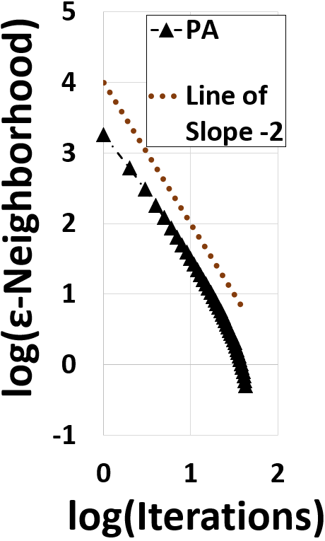
(a) Matrix completion w/ convex (observed quadratic) loss, Schatten-$2$ norm constraint.

(b) Classification w/ quasi-convex (squared sigmoid) loss, $l_{2}$ norm constraint.

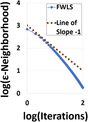
(c) Regression w/ non-convex (bi-weight) loss, $l_{2}$ norm constraint.

Figure 1: Convergence rates of FW variants for convex loss without line search and non-convex loss with line search.

6 Smooth Non-Convex Functions

In this section, we show that, with high probability, FW with line search converges as $O\left(\frac{1}{t}\right)$ to a stationary point when the loss function is non-convex and the constraint set is strongly convex. To our knowledge, a rate this rapid does not exist in the non-convex optimization literature.

To help demonstrate our theoretical guarantee, we introduce a measure called the FW gap. The FW gap of $f$ at a point $w_{t}\in\Omega$ is defined as $k_{t}:=\max_{v\in\Omega}\langle v-w_{t},-\nabla f(w_{t})\rangle$. This measure is adopted in (?), which is the first work to show that, for smooth non-convex functions, FW has an $O\left(\frac{1}{\sqrt{t}}\right)$ convergence rate to a stationary point over arbitrary convex sets. The $O\left(\frac{1}{\sqrt{t}}\right)$ rate matches the rate of projected gradient descent when the loss function is smooth and non-convex. It has been shown (?) that a point $w_{t}$ is a stationary point for the constrained optimization problem if and only if $k_{t}=0$.

Theorem 4.

Assume that the non-convex function $f$ is smooth with parameter $L$ and the constraint set $\Omega$ is $\alpha$-strongly convex and has dimensionality $d$. Further, define the function $h$ as $h(w)=f(w)+\theta\xi^{T}w$ where $\theta\in\left(0,\frac{\epsilon}{4D}\right]$, $\xi\in\mathds{R}^{d}$, $w\in\Omega$, $D$ is the diameter of $\Omega$, and $\xi$ is uniform on the unit sphere. Let $\ell_{1}=f(w_{1})-f(w^{\ast})$ and $C^{\prime}=\frac{\alpha\delta\sqrt{\pi}}{8L\sqrt{2d}}$. Then applying FW with line search to $h$ yields the following guarantee for the FW gap of $f$ with probability $1-\delta$,

$$\underset{1\leq s\leq t}{\min}k_{s}\leq\frac{\ell_{1}}{t\min\{\frac{1}{2},C^{\prime}\}}=O\left(\frac{1}{t}\right)$$

We would further discuss the result stated in the theorem. In non-convex optimization literature, Nesterov and Polyak (?) show that cubic regularization of Newton’s method can find a stationary point in $O(\epsilon^{-3/2})$ iterations and evaluations of the Hessian. First order methods, such as gradient descent, typically require $O(\epsilon^{-2})$ iterations (?) to converge to a stationary point. Recent progress on first order methods, however, assumes some mild conditions and show that an improved rate of $O(\epsilon^{-7/4})$ is possible (?; ?). Here, we show that when the constraint set is strongly convex, FW with line search only needs $O(\epsilon^{-1})$ iterations to arrive within an $\epsilon$-neighborhood of a stationary point. It is important to note, although the $O(\epsilon^{-1})$ convergence rate holds probabilistically, it is quite fast compared to the known rates in the non-convex optimization literature.

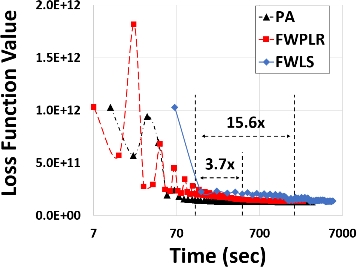
(a) PA vs. standard FW variants.

(b) PA vs. gradient descent.

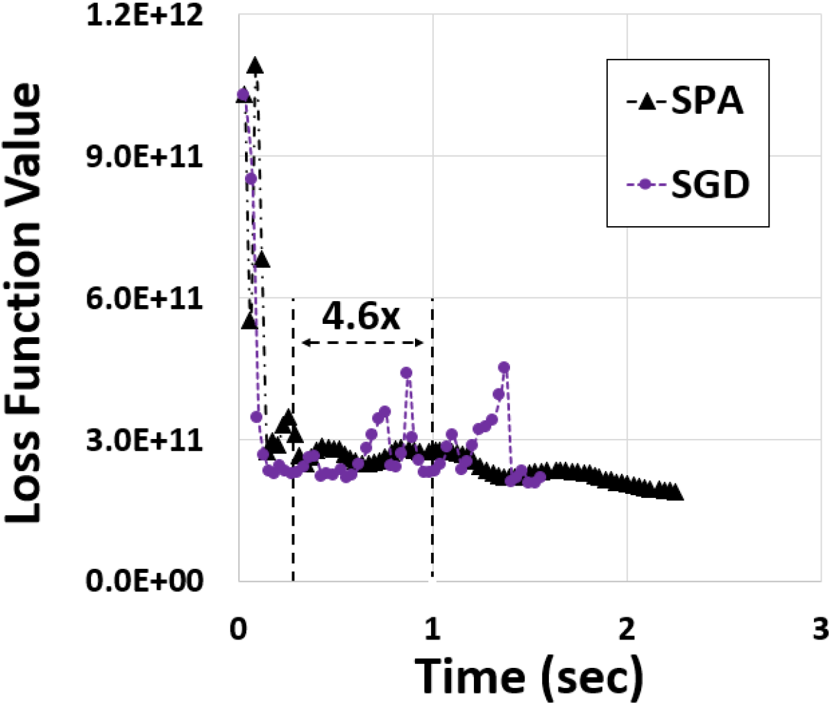
(c) Stochastic PA vs. stochastic GD.

Figure 2: PA versus (a) other FW variants, (b) gradient descent, and (c) stochastic gradient descent.

7 Experiments

We have conducted extensive experiments on different combinations of loss functions, constraint sets, and real-life datasets (Table 2). Here, we only report two main sets of experiments: the empirical validation of our theoretical results in terms of convergence rates (Section 7.1) and the comparison of various optimizations in terms of actual run times (Section 7.2). We refer the interested reader to Appendix B for additional experiments.

For classification and regression, we used the logistic and quadratic loss functions. For matrix completion, we used the observed quadratic loss (?), defined as $f\left(X\right)=\sum_{(i,j)\in P(M)}(X_{i,j}-M_{i,j})^{2}$ where $X$ is the estimated matrix, $M$ is the observed matrix, and $P(M)$$=$$\{(i,j):M_{i,j}\textrm{ is observed}\}$. As a non-convex, but strictly-locally-quasi-convex loss, we also used squared sigmoid loss $\varphi(z)=(1+\exp(-z))^{-1}$ (?) for classification. For robust regression, we used the bi-weight loss (?), as a non-convex (but smooth) loss $\psi(f(x_{i}),y_{i})=\dfrac{(f(x_{i})-y_{i})^{2}}{1+(f(x_{i})-y_{i})^{2}}$.

For regression, we used the YearPredictionMSD dataset (500K observations, 90 features) (?). For classification, we used the Adult dataset (49K observations, 14 features) (?). For matrix completion, we used the MovieLens dataset (1M movie ratings from 6,040 users on 3,900 movies) (?).

7.1 Empirical Validation of Convergence Rates

We ran several experiments to empirically validate our convergence results. In particular, we studied the performance of Primal Averaging (PA) and standard FW With Line Search (FWLS) with both $l_{2}$ and Schatten-$2$ norm balls as our strongly convex constraint sets.

Theorem 1 guarantees a convergence rate of $O(\frac{1}{t^{2}})$ for PA when the constraint set is strongly convex and the loss function is convex. We experimented with both $l_{2}$ (logistic classifier) and Schatten-$2$ norm (matrix completion) balls, measuring the loss value at each iteration. As shown in Figure 1(a), a slope of $-2.41$ confirms Theorem 1’s guarantee, which predicts a slope of at least $-2$.

Theorem 3 shows that FWLS converges to the global minimum at the rate of $O\left(\min\left(\frac{1}{t^{1/3}},\frac{1}{t^{1/2}}\right)\right)$ when the constraint set is strongly convex and the loss function is strictly-locally-quasi-convex. We investigated this result with the squared sigmoid loss and an $l_{2}$ norm constraint. Figure 1(b) exhibits our results, showing a slope of $-2.12$, a finding better than the worst-case bounds given by Theorem 3, i.e., a slope of $-0.5$ (see appendix for a detailed discussion).

From Theorem 4, we expect FWLS to converge to a stationary point of a (smooth) non-convex function at a rate of $O(\frac{1}{t})$ when constrained to a strongly convex set. Using the bi-weight loss and an $l_{2}$ norm constraint, we measured the loss value at each iteration. As shown in Figure 1(c), the results confirmed our theoretical results, showing an even steeper slope ($-1.46$ instead of $-1$, since Theorem 4 only provides a worst-case upper bound).

7.2 Comparison of Different Optimization Algorithms

To compare the actual performance of various optimization algorithms, we measure the run times, instead of the number of iterations to convergence, in order to account for the time spent in each iteration. In Figure 2, dotted vertical lines mark the convergence points of various algorithms.

First, we compared all three variants of FW: PA, standard FW With Predefined Learning Rate (FWPLR) defined in Algorithm 1 with option A, and standard FW With Line Search (FWLS) defined in Algorithm 1 with option B. All methods were tested on a regression task (quadratic loss) with an $\ell_{2}$ norm ball constraint.

As shown in Figure 2(a), PA converged $3.7\times$ and $15.6\times$ faster than FWPLR and FWLS, respectively. This considerable speedup has significant ramifications in practice. Traditionally, PA has been shied away from, due to its slower iterations, while its convergence rate was believed to be the same as the more efficient variants (?). However, as proven in Section 4, PA does converge in fewer iterations.

We also compared the run time of PA versus projected gradient descent (regression task with a quadratic loss). We compared their deterministic versions in Figure 2(b), where PA converged significantly faster ($7.7\times$), as expected. For a fair comparison of their stochastic versions, Stochastic Primal Averaging (SPA) and Stochastic Gradient Descent (SGD), we considered two cases: an $l_{2}$ constraint (which has an efficient projection) and $l_{1.1}$ constraint (which has a costly projection). As expected, for an efficient projection, SGD converged $4.6\times$ faster than SPA (Figure 2(c)), and when the projection was costly, SPA converged $25.1\times$ faster (see Appendix B for detailed plots).

8 Conclusion

In this paper, we revisited an important class of optimization techniques, FW methods, and offered new insight into their convergence properties for strongly convex constraint sets, which are quite common in machine learning. Specifically, we discovered that, for convex functions, a non-conventional variant of FW (i.e., Primal Averaging) converges significantly faster than the commonly used variants of FW with high probability. We also showed that PA’s $O(\frac{1}{t^{2}})$ convergence rate more than compensates for its slightly more expensive computational cost at each iteration. We also proved that for strictly-locally-quasi-convex functions, FW can converge to within an $\epsilon$-neighborhood of the global minimum in $O\left(max(\frac{1}{\epsilon^{2}},\frac{1}{\epsilon^{3}})\right)$ iterations. Even for non-convex functions, we proved that FW’s convergence rate is better than the previously known results in the literature with high probability. These new convergence rates have significant ramifications for practitioners, due to the widespread applications of strongly convex norm constraints in classification, regression, matrix completion, and collaborative filtering. Finally, we conducted extensive experiments on real-world datasets to validate our theoretical results and investigate our improvement over existing methods. In summary, we showed that PA reduces optimization time by $2.8$–$15.6\times$ compared to standard FW variants, and by $7.7$–$25.1\times$ compared to projected gradient descent. Our plan is to integrate PA in machine learning libraries libraries, including our BlinkML project (?).

9 Acknowledgments

This work is in part supported by the National Science Foundation (grants 1629397 and 1553169).

Appendix A Proofs

A.1 Proof of Theorem 1

We begin by providing two lemmas which aid in our proof of Theorem 1. In particular, Lemma 1 allows us to upper-bound the distance between two outputs of the linear oracle by a scaled distance of the oracle’s inputs. Lemma 2 shows that if running PA on an $L$-smooth function $f$ allows $f$ to converge as

$$f(w_{t})-f(w^{*})=O\left(\frac{L}{\alpha^{2}g^{2}t^{2}}\right)$$

then running PA on a perturbed function $h$ allows $f$ to converge as

$$f(w_{t})-f^{*}=O\left(\frac{Ld}{\alpha^{2}\delta^{2}t^{2}}\right)$$

with probability $1-\delta$. Here, $g$ is the smallest value of the norm of averaged gradients and $f^{*}=\underset{w\in\Omega}{\min}f(w)$.

Given this, our proof of Theorem 1 proceeds by first showing that running PA on an $L$-smooth function $f$ over an $\alpha$-strongly convex constraint set $\Omega$ causes $f$ to converge as

$$f(w_{t})-f(w^{*})=O\left(\frac{L}{\alpha^{2}g^{2}t^{2}}\right)$$

We then apply Lemma 2, thereby showing that running PA on a perturbed function $h$ allows $f$ to converge as

$$f(w_{t})-f^{*}=O\left(\frac{Ld}{\alpha^{2}\delta^{2}t^{2}}\right)$$

with probability $1-\delta$.

We now state the Lemmas and provide their proofs.

Lemma 1.

Denote

$$x_{p}=\operatorname*{arg\,max}_{x\in\Omega}\langle p,x\rangle$$

and

$$x_{q}=\operatorname*{arg\,max}_{x\in\Omega}\langle q,x\rangle$$

where $p,q\in\mathds{R}^{d}$ are any non-zero vectors. If a compact set $\Omega$ is an $\alpha$-strongly convex set, then

$$\|x_{p}-x_{q}\|\leq\frac{\left\lVert p-q\right\rVert}{\alpha(\|p\|+\|q\|)}$$ (4)

Proof.

It is shown in Proposition A.1 of (?) that an $\alpha$-strongly convex set can be expressed as the intersection of infinitely many Euclidean balls. Denote the $d$ dimensional unit sphere as ${\mathcal{U}=\left\{u\in\mathds{R}^{d}:\left\lVert u\right\rVert^{2}=1\right\}}$. Furthermore, write $x_{u}=\underset{x\in\Omega}{\operatorname*{arg\,max}}\left\langle x,u\right\rangle$ for some $u\in\mathcal{U}$. Then the $\alpha$-strongly convex set $\Omega$ can be written

$$\Omega=\underset{u\in\mathcal{U}}{\cap}\mathbb{B}_{\frac{1}{\alpha}}\left(x_{u}-\frac{u}{\alpha}\right)$$

Now, let

$${x_{p}=\operatorname*{arg\,max}_{x\in\Omega}\langle\frac{p}{\left\lVert p\right\rVert},x\rangle}$$

and

$${x_{q}=\operatorname*{arg\,max}_{x\in\Omega}\langle\frac{q}{\left\lVert q\right\rVert},x\rangle}$$

Based on the above interpretation of strongly convex sets, we see that

$$x_{q}\in\mathbb{B}_{\frac{1}{\alpha}}(x_{p}-\frac{p}{\alpha\left\lVert p\right\rVert})$$

and

$$x_{p}\in\mathbb{B}_{\frac{1}{\alpha}}(x_{q}-\frac{q}{\alpha\left\lVert q\right\rVert})$$

Therefore,

$$\|x_{q}-x_{p}-\frac{p}{\alpha\left\lVert p\right\rVert}\|^{2}\leq\frac{1}{\alpha^{2}}$$

which leads to

$$\|x_{p}-x_{q}\|^{2}\leq\frac{2}{\alpha}\langle x_{p}-x_{q},\frac{p}{\|p\|}\rangle$$ (5)

and

$$\|x_{p}-x_{q}-\frac{q}{\alpha\|q\|}\|^{2}\leq\frac{1}{\alpha^{2}}$$

which results in

$$\|x_{p}-x_{q}\|^{2}\leq\frac{2}{\alpha}\langle x_{q}-x_{p},\frac{q}{\|q\|}\rangle$$ (6)

Summing (5) and (6) then applying the Cauchy-Schwarz inequality completes the proof. ∎

We note that Lemma 1 also implies that the sub-gradient of the linear oracle’s output is Lipschitz continuous. We now present Lemma 2.

Lemma 2.

Given $f:\mathds{R}^{d}\rightarrow\mathds{R},w,\xi\in\mathds{R}^{d}$, and $\theta\in\mathds{R}$, denote $h(w)=f(w)+\theta\xi^{T}w$. Let $\xi$ be uniform on the unit sphere and $\theta>0$. Then with probability $1-\delta$,

$$\frac{\delta\sqrt{\pi}}{\sqrt{2d}}\leq\left\lVert\nabla h(w)\right\rVert$$

Further, if $h$ is smooth with parameter $L$ and applying PA to $h$ over an $\alpha$-strongly convex constraint set $\Omega$ allows $h$ to converge as

$$h(w_{t})-h^{*}=O\left(\frac{L}{\alpha^{2}g^{2}t^{2}}\right)$$

then it also holds that

$$f(w_{t})-f^{*}=O\left(\frac{Ld}{\alpha^{2}\delta^{2}t^{2}}\right)$$

with probability $1-\delta$.

Proof.

Note that $\left\lVert\nabla h(w)\right\rVert\geq\left|\nabla h(w)[1]\right|$ where $y[i]$ is the $i$th component of $y\in\mathds{R}^{d}$. Since $\nabla h(w)[1]=\nabla f(w)[1]+\theta\xi[1]$,

$$Pr\left(\nabla h(w)[1]\leq\frac{\theta\delta\sqrt{\pi}}{\sqrt{2d}}\right)\leq Pr\left(\xi[1]\leq\frac{\delta\sqrt{\pi}}{\sqrt{2d}}\right)\leq\delta$$

as $\xi[1]\sim Beta(\frac{1}{2},\frac{d-1}{2})$. Thus, we can lower bound the gradient norm by $\frac{\delta\sqrt{\pi}}{\sqrt{2d}}$ with probability $1-\delta$.

Now, denote

$$h^{*} =\underset{w\in\Omega}{\min}h(w)$$

$$w^{*} =\underset{w\in\Omega}{\operatorname*{arg\,min}}f(w)$$

Recall our assumption that $h$ is smooth with parameter $L$ and that applying PA to $h$ causes $h$ to converge as

$$h(w_{t})-h^{*}=O\left(\frac{L}{\alpha^{2}g^{2}t^{2}}\right)$$

Note that $g\geq\frac{\delta\sqrt{\pi}}{\sqrt{2d}}\geq 0$, so

$$h(w_{t})-h^{*}=O(\frac{Ld}{\alpha^{2}\delta^{2}t^{2}})$$

Further, observe that by the construction of $h$ we have

$$\left|f(w)-h(w)\right|\leq\theta\left\lVert w\right\rVert$$ (7)

for any $w$. Now, whenever $h(w_{t})-h^{*}=O(\frac{Ld}{\alpha^{2}\delta^{2}t^{2}})=\epsilon$ we see that

$$f(w_{t}) \leq f(w_{t})+\theta\left\lVert w_{t}\right\rVert$$

$$\leq h^{*}+\epsilon+\theta\left\lVert w_{t}\right\rVert$$

$$\leq h(w^{*})+\epsilon+\theta\left\lVert w_{t}\right\rVert$$

$$\leq f(w^{*})+\epsilon+\theta(\left\lVert w_{t}\right\rVert+\left\lVert w^{*}\right\rVert)$$

$$\leq f(w^{*})+\epsilon+2\theta D$$

$$\leq f(w^{*})+1.5\epsilon$$

The first and third lines follow from (7), the second from $h^{*}$ being the minimum value of $h$, the fourth from $D$ being the diameter of the constraint set, and fifth from the choice of $\theta=\frac{\epsilon}{4D}$. Thus we obtain the convergence rate of $O\left(\frac{Ld}{\alpha^{2}\delta^{2}t^{2}}\right)$ for $f$ with probability $1-\delta$. ∎

We now proceed with our proof of Theorem 1.

Proof.

According to Theorem 8 in (?), we already have

$$f(w_{t})-f(w^{\ast})\leq\frac{2L}{t(t+1)}\sum_{\tau=1}^{t}\left\lVert v_{\tau}-v_{\tau-1}\right\rVert^{2}$$ (8)

Fix a $t$. Denote

$$p_{t}=\frac{1}{\Theta_{t}}\sum_{i=1}^{t}\theta_{i}\nabla f(z_{i-1})$$

and

$$p_{t-1}=\frac{1}{\Theta_{t-1}}\sum_{i=1}^{t-1}\theta_{i}\nabla f(z_{i-1})$$

By using Lemma 1, we have

$$\|v_{t}-v_{t-1}\|\leq\frac{\left\lVert p_{t}-p_{t-1}\right\rVert}{\alpha(\|p_{t}\|+\|p_{t-1}\|)}$$ (9)

Based on the update rule

$$p_{t} =\Theta_{t}^{-1}(p_{t-1}\Theta_{t-1}+\theta_{t}\nabla f(z_{t-1}))$$ (10)

$$=\frac{\Theta_{t}-\theta_{t}}{\Theta_{t}}p_{t-1}+\frac{\theta_{t}}{\Theta_{t}}\nabla f(z_{t-1})$$

So

$$p_{t}-p_{t-1}=\gamma_{t}(\nabla f(z_{t-1})-p_{t-1})$$

given that $\gamma_{t}=\frac{\theta_{t}}{\Theta_{t}}$. By substituting the result back into (9) and noting that $\gamma_{t}=O\left(\frac{1}{t}\right)$, we find that

$$\|v_{t}-v_{t-1}\| \leq\frac{\gamma_{t}(\|p_{t-1}\|+\|\nabla f(z_{t-1})\|)}{\alpha(\|p_{t}\|+\|p_{t-1}\|)}$$ (11)

$$=O(\frac{1}{\alpha gt}),\forall t$$

By combining (8) and (11), we get

$$f(w_{t})-f(w^{\ast}) \leq\frac{2L}{t(t+1)}\overset{t}{\underset{\tau=1}{\Sigma}}\|v_{\tau}-v_{\tau-1}\|^{2}$$ (12)

$$\leq\frac{2L}{t(t+1)}\Sigma_{i=1}^{t}O(\frac{1}{\alpha^{2}g^{2}i^{2}})$$

$$=O(\frac{L}{\alpha^{2}g^{2}t^{2}})$$

where we used the fact that $\sum_{i=1}^{\infty}\frac{1}{i^{2}}=\frac{\pi}{6}$ in the final equality.

Finally, applying the result of Lemma 2 yields with probability $1-\delta$ the convergence rate $f(w_{t})-f(w^{*})=O\left(\frac{Ld}{\alpha^{2}\delta^{2}t^{2}}\right)$ as claimed. ∎

A.2 Proof of Theorem 2

Proof.

We note that

$$f(\mathbf{w}_{t}) \leq f(\mathbf{z}_{t-1})+\langle\nabla f(\mathbf{z}_{t-1}),\mathbf{w}_{t}-\mathbf{z}_{t-1}\rangle$$ (13)

$$\quad+\frac{L}{2}\|\mathbf{w}_{t}-\mathbf{z}_{t-1}\|^{2}$$

$$\overset{(0)}{=}(1-\gamma_{t})[f(\mathbf{z}_{t-1})+\langle\nabla f(\mathbf{z}_{t-1}),\mathbf{w}_{t-1}-\mathbf{z}_{t-1}\rangle]$$

$$\quad+\gamma_{t}[f(\mathbf{z}_{t-1})+\langle\nabla f(\mathbf{z}_{t-1}),\mathbf{v}_{t}-\mathbf{z}_{t-1}\rangle]$$

$$\quad+\frac{L\gamma_{t}^{2}}{2}\|\mathbf{v}_{t}-\mathbf{v}_{t-1}\|^{2}$$

$$\overset{(1)}{\leq}(1-\gamma_{t})f(\mathbf{w}_{t-1})+\gamma_{t}[f(\mathbf{z}_{t-1})$$

$$\quad+\langle\nabla f(\mathbf{z}_{t-1}),\mathbf{v}_{t}-\mathbf{z}_{t-1}\rangle]+\frac{L\gamma_{t}^{2}}{2}\|\mathbf{v}_{t}-\mathbf{v}_{t-1}\|^{2}$$

$$=(1-\gamma_{t})f(\mathbf{w}_{t-1})+\gamma_{t}[f(\mathbf{z}_{t-1})$$

$$\quad+\langle\tilde{\nabla}f(\mathbf{z}_{t-1}),\mathbf{v}_{t}-\mathbf{z}_{t-1}\rangle]+\frac{L\gamma_{t}^{2}}{2}\|\mathbf{v}_{t}-\mathbf{v}_{t-1}\|^{2}$$

$$\quad+\gamma_{t}\langle\nabla f(\mathbf{z}_{t-1})-\tilde{\nabla}f(\mathbf{z}_{t-1}),\mathbf{v}_{t}-\mathbf{z}_{t-1}\rangle$$

$$\overset{(2)}{\leq}(1-\gamma_{t})f(\mathbf{w}_{t-1})+\gamma_{t}[f(\mathbf{z}_{t-1})$$

$$\quad+\langle\tilde{\nabla}f(\mathbf{z}_{t-1}),\mathbf{w}^{\ast}-\mathbf{z}_{t-1}\rangle]+\frac{L\gamma_{t}^{2}}{2}\|\mathbf{v}_{t}-\mathbf{v}_{t-1}\|^{2}$$

$$\quad+\gamma_{t}\langle\nabla f(\mathbf{z}_{t-1})-\tilde{\nabla}f(\mathbf{z}_{t-1}),\mathbf{v}_{t}-\mathbf{z}_{t-1}\rangle$$

$$=(1-\gamma_{t})f(\mathbf{w}_{t-1})+\gamma_{t}[f(\mathbf{z}_{t-1})$$

$$\quad+\langle\nabla f(\mathbf{z}_{t-1}),\mathbf{w}^{\ast}-\mathbf{z}_{t-1}\rangle]+\frac{L\gamma_{t}^{2}}{2}\|\mathbf{v}_{t}-\mathbf{v}_{t-1}\|^{2}$$

$$\quad+\gamma_{t}\langle\nabla f(\mathbf{z}_{t-1})-\tilde{\nabla}f(\mathbf{z}_{t-1}),\mathbf{v}_{t}-\mathbf{w}^{\ast}\rangle$$

$$\overset{(3)}{\leq}(1-\gamma_{t})f(\mathbf{w}_{t-1})+\gamma_{t}f(\mathbf{w}^{\ast})$$

$$\quad+\gamma_{t}\langle\nabla f(\mathbf{z}_{t-1})-\tilde{\nabla}f(\mathbf{z}_{t-1}),\mathbf{v}_{t}-\mathbf{w}^{\ast}\rangle$$

$$\quad+\frac{L\gamma_{t}^{2}}{2}\|\mathbf{v}_{t}-\mathbf{v}_{t-1}\|^{2}$$

$(0)$ follows from the fact that, as $\mathbf{w}_{t}=(1-\gamma_{t})\mathbf{w}_{t-1}+\gamma_{t}\mathbf{v}_{t}$ and $\mathbf{z}_{t-1}=(1-\gamma_{t})\mathbf{w}_{t-1}+\gamma_{t}\mathbf{v}_{t-1}$,

$$\mathbf{w}_{t}-\mathbf{z}_{t-1}=\gamma_{t}(\mathbf{v}_{t}-\mathbf{v}_{t-1})$$ (14)

Furthermore, $(1)$ is implied by the convexity of $f$, $(2)$ follows from the application of the linear oracle, and $(3)$ follows again from the convexity of $f$. Moreover, by taking the expectation over the randomness, we find that

$$E[f(\mathbf{w}_{t})] \leq(1-\gamma_{t})f(\mathbf{w}_{t-1})+\gamma_{t}f(\mathbf{w}^{\ast})$$ (15)

$$\quad+\frac{L\gamma_{t}^{2}}{2}\|\mathbf{v}_{t}-\mathbf{v}_{t-1}\|^{2}+\gamma_{t}\frac{\sigma D}{\sqrt{n_{t}}}$$

since

$$E[\| \nabla f(\mathbf{z}_{t-1})-\tilde{\nabla}f(\mathbf{z}_{t-1})\|]$$ (16)

$$\leq\sqrt{E[\|\nabla f(\mathbf{z}_{t-1})-\tilde{\nabla}f(\mathbf{z}_{t-1})\|]^{2}}$$

$$\leq\sigma/\sqrt{n_{t}}$$

To maintain an $O(\frac{1}{t^{2}})$ convergence rate, $\frac{\sigma D\gamma_{t}}{\sqrt{n_{t}}}$ must decay as ${\frac{L\gamma_{t}^{2}}{2}\|\mathbf{v}_{t}-\mathbf{v}_{t-1}\|^{2}}$. Recall that the latter term is $O\left(\frac{1}{t^{4}}\right)$. This implies that $n_{t}$ must be $O(t^{6})$ so that $\gamma_{t}\frac{\sigma D}{\sqrt{n_{t}}}$ can decay as $O\left(\frac{1}{t^{4}}\right)$. However, if $n_{t}=O(t^{4})$, stochastic Primal Averaging yields the slightly worse $O\left(\frac{\log t}{t^{2}}\right)$ convergence rate.

Finally, we can remove the reliance on the $\underset{1\leq s\leq t}{\min}\left\lVert\nabla f(z_{s})\right\rVert+\left\lVert\nabla f(z_{s-1})\right\rVert$ term in the convergence rate by repeating the analysis given in Lemma 2. As this analysis is very similar to the previously provided analysis of Lemma 2, it is omitted. Then when $n_{t}=O(t^{4})$ we have with probability $1-\delta$

$$E[f(w_{t})]-f^{*}=O\left(\frac{dL^{2}(D^{2}+\sigma)\log t}{\alpha^{2}\delta^{2}t^{2}}\right)$$

∎

A.3 Proof of Theorem 3

We state the following lemma from (?).

Lemma 3.

Write the dual norm as $\left\lVert\cdot\right\rVert_{\ast}$. For iteration $t$ of FW with line search, if ${L<\frac{\alpha\|\nabla f(w_{t})\|_{\ast}}{4}}$ set $\gamma_{t}=1$; otherwise, set ${\gamma_{t}=\frac{\alpha\|\nabla f(w_{t})\|_{\ast}}{4L}}$. Then, under the conditions of Theorem 3, Algorithm 1 option (B) has the following guarantee:

$$f(w_{t+1})\leq f(w_{t})+\frac{\gamma_{t}}{2}\langle w^{\ast}-w_{t},\nabla f(w_{t})\rangle$$

We use Lemma 3 to prove Theorem 3.

Proof.

Assume that,

$$f(w_{t})-f(w^{*})>\epsilon$$

Otherwise, the algorithm has reached the $\epsilon$-neighborhood of $w^{*}$. By the strictly-locally-quasi-convexity of $f$, we must have,

$$\|\nabla f(w)\|>0$$

and for every $x\in\mathbb{B}_{\epsilon/\kappa}(w)$ it holds that,

$$\langle\nabla f(w),x-w\rangle\leq 0$$

Now choose a point $y$ such that,

$$y=w^{*}+\frac{\epsilon\nabla f(w_{t})}{\kappa\|\nabla f(w_{t})\|}$$

and,

$$y\in\mathbb{B}_{\epsilon/\kappa}(w^{*})$$

Then we have the following,

$$\hskip 13.30003pt\langle\frac{\nabla f(w_{t})}{\|\nabla f(w_{t})\|},y-w_{t}\rangle\leq 0$$ (17)

$$\equiv\langle\frac{\nabla f(w_{t})}{\|\nabla f(w_{t})\|},\frac{\epsilon\nabla f(w_{t})}{\kappa\|\nabla f(w_{t})\|}+w^{*}-w_{t}\rangle\leq 0$$

$$\equiv\langle\frac{\nabla f(w_{t})}{\|\nabla f(w_{t})\|},w_{t}-w^{*}\rangle\geq\frac{\epsilon}{\kappa}$$

$$\equiv\langle\nabla f(w_{t}),w_{t}-w^{*}\rangle\geq\frac{\epsilon}{\kappa}\|\nabla f(w_{t})\|$$

Case 1: ($L<\frac{\alpha\|\nabla f(w_{t})\|_{\ast}}{4}$. Set $\gamma_{t}=1$):

$$f(w_{t+1}) \leq f(w_{t})+\frac{\gamma_{t}}{2}\langle\nabla f(w_{t}),w^{\ast}-w_{t}\rangle$$ (18)

$$\overset{(\ref{eq:5})}{\leq}f(w_{t})-\frac{\gamma_{t}\epsilon}{2\kappa}\|\nabla f(w_{t})\|$$

$$=f(w_{t})-\frac{\epsilon}{2\kappa}\|\nabla f(w_{t})\|$$

Case 2: ($L\geq\frac{\alpha\|\nabla f(w_{t})\|_{\ast}}{4}$. Set $\gamma_{t}=\frac{\alpha\|\nabla f(w_{t})\|_{\ast}}{4L}$):

$$f(w_{t+1}) \leq f(w_{t})+\frac{\gamma_{t}}{2}\langle\nabla f(w_{t}),w^{\ast}-w_{t}\rangle$$ (19)

$$=f(w_{t})+\frac{\alpha\|\nabla f(w_{t})\|_{\ast}}{16L}\langle\nabla f(w_{t}),w^{\ast}-w_{t}\rangle$$

$$\overset{(\ref{eq:5})}{=}f(w_{t})-\frac{\alpha\epsilon\|\nabla f(w_{t})\|_{\ast}\|\nabla f(w_{t})\|}{8\kappa L}$$

$$\leq f(w_{t})-\frac{\alpha\epsilon\|\nabla f(w_{t})\|^{2}_{2}}{8\kappa L}$$

By (18) and (19), we observe that the loss function monotonically decreases until it enters an $\epsilon$-neighborhood of the global minimum, thereby proving that FW with line search can converge within an $\epsilon$-neighborhood of the global minimum. To prove that the algorithm requires $t=O(max(\frac{1}{\epsilon^{2}},\frac{1}{\epsilon^{3}}))$, we use the additional assumption,

$$f(w)-f(w^{*})\geq\epsilon\rightarrow\|\nabla f(w)\|\geq\theta\epsilon$$

Now, assume that after iteration $t$ the algorithm reaches the target $\epsilon$-neighborhood. Denote the solution vector at iteration $t$ as $w_{t}$. Then, in case (1), we have,

$$f(w_{t})\leq f(w_{1})-\frac{t\epsilon^{2}\theta}{2\kappa}$$ (20)

or

$$t \leq\frac{2\kappa(f(w_{1})-f(w_{t}))}{\epsilon^{2}\theta}$$ (21)

$$\leq\frac{2\kappa(f(w_{1})-f(w^{*}))}{\epsilon^{2}\theta}$$

while for case (2), we have,

$$f(w_{t})\leq f(w_{1})-\frac{t\epsilon^{3}\theta}{8\kappa L}$$ (22)

or

$$t \leq\frac{8L\kappa(f(w_{1})-f(w_{t}))}{\epsilon^{3}\theta}$$ (23)

$$\leq\frac{8L\kappa(f(w_{1})-f(w^{*}))}{\epsilon^{3}\theta}$$

This shows that it requires ${t=O\left(max\left(\frac{1}{\epsilon^{2}},\frac{1}{\epsilon^{3}}\right)\right)}$ iterations for the algorithm to produce an iterate that is within the $\epsilon-$neighborhood of the global minimum.

∎

A.4 Proof of Theorem 4

Proof.

Let $w_{\gamma}=w_{t}+\gamma(p_{t}-w_{t})$ for some $\gamma\in[0,1]$. Then, $f(w_{t+1})\leq f(w_{\gamma})$ as $w_{t+1}$ is obtained by line search and thus uses an optimal step size.

$$f(w_{t+1}) \leq f(w_{\gamma})$$ (24)

$$\leq f(w_{t})+\gamma\langle\nabla f(w_{t}),v_{t}-w_{t}\rangle$$

$$\quad+\frac{\gamma^{2}L\left\lVert v_{t}-w_{t}\right\rVert^{2}}{2}$$

$$\overset{(0)}{\leq}f(w_{t})+\gamma\langle c_{t}-w_{t},\nabla f(w_{t})\rangle$$

$$\quad+\frac{\gamma^{2}L\left\lVert v_{t}-w_{t}\right\rVert^{2}}{2}$$

where (0) follows from $v_{t}=\operatorname*{arg\,min}_{v\in X}\langle\nabla f(w_{t}),v\rangle$. Let $c_{t}$ above be,

$$c_{t}=\frac{u_{t}+v_{t}}{2}+\frac{\alpha w_{t}\left\lVert w_{t}-v_{t}\right\rVert^{2}}{8}$$

where $c_{t}\in\Omega$ by the definition of a strongly convex set. Let us write,

$$u_{t}=\operatorname*{arg\,min}_{\|u\|\leq 1}\langle u,\nabla f(w_{t})\rangle=-\|\nabla f(w_{t})\|_{\ast}$$

where the last equality is obtained by the definition of the dual norm. Then,

$$\langle c_{t}-w_{t},\nabla f(w_{t})\rangle \leq\frac{1}{2}\langle v_{t}-w_{t},\nabla f(w_{t})\rangle$$ (25)

$$\quad+\frac{\alpha}{8}\langle\|v_{t}-w_{t}\|^{2}u_{t},\nabla f(w_{t})\rangle$$

$$\leq\frac{1}{2}\langle v_{t}-w_{t},\nabla f(w_{t})\rangle$$

$$\quad-\frac{\alpha}{8}\|v_{t}-w_{t}\|^{2}\|\nabla f(w_{t})\|_{\ast}$$

$$=-\frac{k_{t}}{2}-\frac{\alpha}{8}\|v_{t}-w_{t}\|^{2}\nabla\|f(w_{t})\|_{\ast}$$

where the last line is due to the definition of the FW gap. Combining (24) and (25) gives,

$$f(w_{t+1})\leq f(w_{t})-\frac{\gamma k_{t}}{2}+\frac{\|v_{t}-w_{t}\|^{2}}{2}(\gamma^{2}L-\gamma\frac{\alpha\|\nabla f(w_{t})\|_{\ast}}{4})$$

Case 1: $L\leq\frac{\alpha\|\nabla f(w_{t})\|_{\ast}}{4}$, set $\gamma=1$, we get,

$$f(w_{t+1})\leq f(w_{t})-\frac{k_{t}}{2}$$

Case 2: $L\geq\frac{\alpha\|\nabla f(w_{t})\|_{\ast}}{4}$, set $\gamma=\frac{\alpha\|\nabla f(w_{t})\|_{\ast}}{4L}$, we get,

$$f(w_{t+1})\leq f(w_{t})-\frac{\alpha k_{t}\|\nabla f(w_{t})\|_{\ast}}{8L}$$

By recursively applying the above inequality, we get,

$$f(w_{t+1})\leq f(w_{1})-\sum_{s=1}^{t}\min\left(\frac{k_{s}}{2},\frac{\alpha k_{s}\|\nabla f(w_{s})\|_{\ast}}{8L}\right)$$

Denote, $\tilde{k}_{t}=\underset{1\leq s\leq t}{\min}k_{s}.$ We have,

$$f(w_{t+1})\leq f(w_{1})-\tilde{k}_{t}\sum_{s=1}^{t}\min\left(\frac{1}{2},\frac{\alpha\|\nabla f(w_{s})\|_{\ast}}{8L}\right)$$ (26)

Furthermore, if we assume that,

$$\|\nabla f(w_{s})\|_{\ast}\geq c>0,\forall s$$ (27)

then,

$$\tilde{k}_{t}\leq\frac{(f(w_{1})-f(w_{t}))}{t\min\{\frac{1}{2},\frac{\alpha c}{8L}\}}$$

Since $f(w_{1})-f(w_{t})\leq f(w_{1})-f(w^{\ast})=\ell_{1}$, we get,

$$\tilde{k}_{t}\leq\frac{\ell_{1}}{t\min\{\frac{1}{2},C^{\prime}\}}$$

where $C^{\prime}=\frac{\alpha c}{8L}$.

Finally, by repeating the analysis of Lemma 2 we find with probability $1-\delta$ that $c\leq\frac{\delta\sqrt{\pi}}{\sqrt{2d}}$ and thus

$$\tilde{k}_{t}\leq\frac{\ell_{1}}{t\min\{\frac{1}{2},C^{\prime}\}}$$

for $C^{\prime}=\frac{\alpha\delta\sqrt{\pi}}{8L\sqrt{2d}}$.

∎

Appendix B Additional Experiments

In this appendix, we provide a more detailed version of our experimental results. Our experiments aim to answer the following questions:

1. In what situations do the projections become a performance bottleneck for gradient descent algorithms? (Section B.2)

2. When optimizing convex functions over strongly convex sets, does Primal Averaging (PA) outperform standard FW in practice (as our theory from Section 4 suggests)? If so, by how much? (Sections B.3 and B.4)

3. Does PA also outperform projected gradient descent when optimizing convex functions over strongly convex sets? If so, by how much? (Section B.5)

4. For strictly-locally-quasi-convex loss functions (?), does FW’s convergence rate in practice match our theoretical results from Section 5? (Section B.6)

5. When optimizing non-convex loss functions, how fast does FW converge in practice? Does it match our results from Section 6? (Section B.7)

In summary, our empirical results show the following:

1. Projections are costly and responsible for a considerable portion of the overall runtime of gradient descent, whenever the projection step has no closed-form solution (e.g., when the constraint set is an $l_{1.5}$ ball), or when the closed-form solution itself is expensive (e.g., projecting a matrix onto a nuclear norm ball, which requires computing the SVD (?)).

2. In practice, the convergence rate of primal averaging matches our theoretical result of $O(\frac{1}{t^{2}})$ for smooth, convex functions with a strongly convex constraint set. Furthermore, under these conditions, primal averaging outperforms FW both with and without line search by $3.7$–$15.6\times$ for a regression task and $2.8$–$11.7\times$ for a matrix completion task in terms of the overall optimization time. It also outperforms projected gradient descent by $7.7\times$ and can outperform stochastic gradient descent by up to $25.1\times$.

3. When optimizing strictly-locally-quasi-convex functions over strongly convex constraint sets, FW with line search converges to an $\epsilon$-neighborhood of the global minimum within $O(\max(\frac{1}{\epsilon^{2}},\frac{1}{\epsilon^{3}}))$ iterations, as predicted by Theorem 3.

4. When the loss function is non-convex but the constraint set is strongly convex, FW with line search converges to a stationary point at a convergence rate of $O(\frac{1}{t})$, as predicted by Theorem 4.

B.1 Experiment Setup

Hardware and Software — Unless stated otherwise, all experiments were conducted on a Red Hat Enterprise Linux 7.1 server with 112 Intel(R) Xeon(R) CPU E7-4850 v3 processors and 2.20GHz cores and 1T DDR4 memory. All algorithms were implemented in Matlab R2015a. For projections that required solving a convex optimization problem, we used the CVX package (?; ?).

Convexity of Loss Function	Loss Function	Constraint	Task
Convex	Logistic Loss	$l_{p}$ norm	Classification
	Quadratic Loss	$l_{p}$ norm	Regression
	Observed Quadratic Loss	Schatten-$p$ norm	Matrix Completion
Strictly-Locally-Quasi-Convex	Squared Sigmoid	$l_{p}$ norm	Classification
Non-Convex	Bi-Weight Loss	$l_{p}$ norm	Robust Regression

Table 3: Various loss functions and constraint sets used in our experiments.

Loss Functions — In our experiments, we used a variety of popular loss functions to cover various types of convexity and different types of machine learning tasks used in practice. These functions, summarized in Table 3, are as follows.

• Logistic Loss. Logistic regression uses a convex loss function, which is also commonly used in classification tasks (?) and is defined as:

  $$\ell(f(x_{i}),y_{i})=\log(1+e^{-y_{i}f(x_{i})})$$ (28)

  where $f$ is a hypothesis function for the learning task and $y_{i}$ is the target value corresponding to $x_{i}$. Logistic loss is often used with an $l_{p}$ norm constraint to avoid overfitting (?). The optimization problem is thus stated as follows:

  $$\underset{w\in\mathbb{R}^{d},b\in\mathbb{R}}{\min}\text{ }\sum_{i=1}^{N}\ell\left(w^{T}x_{i}+b,y_{i}\right)$$ (29)

  $$\text{ s.t. }\|w\|_{p}\leq r.$$

  where $w$ is the coefficient vector, $b$ is the linear offset, $N$ is the number of data points, and $r$ is the radius of the $l_{p}$ norm ball.

• Quadratic Loss. The quadratic loss is a convex loss function and is commonly used in regression tasks (a.k.a. least squares loss) (?):

  $$\psi(f(x_{i}),y_{i})=(f(x_{i})-y_{i})^{2}$$ (30)

  Similar to logistic regression, a typical choice of constraint here is the $l_{p}$ norm. The optimization is stated as follows:

  $$\underset{w\in\mathbb{R}^{d},b\in\mathbb{R}}{\min}\text{ }\sum_{i}\psi\left(w^{T}x_{i}+b,y_{i}\right)$$ (31)

  $$\text{ s.t. }\|w\|_{p}\leq r.$$

• Observed Quadratic Loss. This loss function is also convex, but is typically used in matrix completion tasks (?), and is defined as:

  $$\|X-M\|_{OB}^{2}=\sum_{(i,j)\in P(M)}(X_{i,j}-M_{i,j})^{2},$$ (32)

  where $X,M\in\mathbb{R}^{m\times n}$, $X$ is the estimated matrix, $M$ is the observed matrix, and $P(M)=\{(i,j):M_{i,j}\textrm{ is observed}\}$. In matrix completion, the loss function is often constrained within a Schatten-$p$ norm ball (?; ?; ?), which is a convex constraint set. Here, the optimization problem is stated as follows:

  $$\underset{X\in\mathbb{R}^{m\times n}}{\min}\text{ }\|{X-M}\|_{OB}^{2}$$ (33)

  $$\text{ s.t. }\|X\|_{\mathbb{S}_{p}}\leq r$$

  where $\|\cdot\|_{\mathbb{S}_{p}}$ is the Schatten-$p$ norm.

• Squared Sigmoid Loss. This function is non-convex, but it is strictly-locally-quasi-convex (see Section 3.1.1 of (?)), and is defined as:

  $$\varphi(z)=(1+\exp(-z))^{-1}$$ (34)

  where $z\in\mathbb{R}^{n}$. We can state the optimization problem as follows:

  $$\underset{w\in\mathbb{R}^{d},b\in\mathbb{R}}{\min}\text{ }\frac{1}{n}\sum_{i}^{n}(y_{i}-\varphi\left(w^{T}x_{i}+b)\right)^{2}$$ (35)

  $$\text{ s.t. }\|w\|_{p}\leq r.$$

  where $n$ is the number of data points.

• Bi-Weight Loss. This loss function is non-convex, and is defined as follows:

  $$\phi(f(x_{i}),y_{i})=\dfrac{(f(x_{i})-y_{i})^{2}}{1+(f(x_{i})-y_{i})^{2}}$$ (36)

  The bi-weight loss is typically used for robust regression tasks (?). Using the $l_{p}$ norm as a constraint, the optimization problem here is stated as follows:

  $$\underset{w\in\mathbb{R}^{d},b\in\mathbb{R}}{\min}\text{ }\sum_{i}\phi\left(w^{T}x_{i}+b,y_{i}\right)$$ (37)

  $$\text{ s.t. }\|w\|_{p}\leq r.$$

Datasets — We ran our experiments using several datasets of different sizes and dimensionalities:

• For regression tasks, we used the YearPredictionMSD dataset (?), comprised of 515,345 observations and 90 real-valued features (428 MB in size). The regression goal is to predict the year a song was released based on its audio features.

• For classification tasks, we used the well-known Adult dataset (?), which offers various demographics (14 features) about 48,842 individuals across the United States. The goal is to predict whether an individual earns more than $50K per year, given his/her demographics.

• For matrix completion tasks, we used two versions of the MovieLens dataset (?), one with 100K observations of movie ratings from 943 users on 1682 movies, and the other with 1M observations of movie ratings from 6,040 users on 3,900 movies.

Compared Methods — We compared different variants of both gradient descent as well as FW optimization:

• Standard Gradient Descent (GD). In the $k^{th}$ iteration, GD moves the opposite direction of the gradient:

  $$w^{(k+1)}=w^{(k)}-\eta\sum_{x_{i}}\nabla f(x_{i})$$ (38)

  where $f(x_{i})$ is the loss on data point $x_{i}$.

• Stochastic Gradient Descent (SGD). Unlike GD, SGD uses only one data point in each iteration:

  $$w^{(k+1)}=w^{(k)}-\eta\nabla f(x_{k+1})$$ (39)

• Standard Frank-Wolfe with Predefined Learning Rate (FWPLR). This variant of Frank-Wolfe corresponds to Algorithm 1 with option (A).

• Standard Frank-Wolfe with Line Search (FWLS). This corresponds to Algorithm 1 with option (B).

• Primal Averaging (PA). Primal averaging is the variant of FW algorithm, which we advocate in this paper. This algorithm was presented in Algorithm 2.

• Stochastic Primal Averaging (SPA). This is the stochastic version of PA, as described in Section 4.2.

B.2 Projection Overhead in Gradient Descent

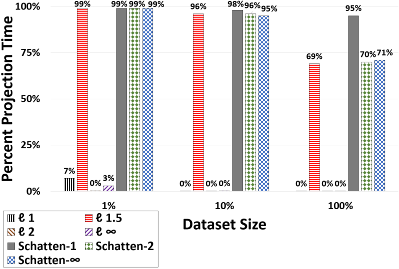
Figure 3: The amount of overall time spent on projection in gradient descent.

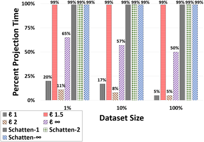
Figure 4: The amount of overall time spent on projection in stochastic gradient descent.

To understand the overhead of the projection step in gradient descent algorithm, we experimented with various machine learning tasks and constraint sets. Specifically, we studied $l_{1}$, $l_{1.5}$, $l_{2}$, $l_{\infty}$, Schatten-$1$, Schatten-$2$, and Schatten-$\infty$ norms as our constraint sets. We used the $l_{p}$ norm balls in a logistic loss classifier (Adult dataset) and used the Schatten-$p$ norms in a matrix completion task (MovieLens dataset) with observed quadratic loss (see Section B.1 and Table 3). To study the effect of data size, we also ran each experiment using different portions of its respective dataset: 1%, 10%, and 100%.

These constraint sets can be divided into three categories (?): (i) projection onto the $l_{1}$, $l_{2}$, and $l_{\infty}$ balls have a closed-form and thus can be computed efficiently, (ii) projection onto Schatten-$1$ (a.k.a. nuclear or trace norm), Schatten-$2$, and Schatten-$\infty$ norms has a closed-form but the closed-form requires the SVD of the model matrix, and is thus costly, and (iii) projection onto $l_{1.5}$ balls does not have any closed-form and requires solving another optimization problem.

Figure 3 shows the average portion of the total time spent in each iteration of the gradient descent in performing the projection step. As expected, the projection step did not account for much of the overall runtime when there was an efficient closed-form, i.e., less than $7\%$, $0.03\%$, and $3\%$ for the $l_{1}$, $l_{2}$, and $l_{\infty}$ norms, respectively. In contrast, projections that involved a costly closed-form or required solving a separate optimization problem introduced a significant overhead. Specifically, the projection time was responsible for 69–99% of the overall runtime for $l_{1.5}$, $95$–$99\%$ for Schatten-$1$, $70$–$99\%$ for Schatten-$2$, and $71$–$99\%$ for Schatten-$\infty$.

Another observation is that this overhead decreased with the data size. This is expected, as the cost of computing the gradient itself in GD grows with the data size and becomes the dominating factor, hence reducing the relative ratio of the projection time to the overall runtime of each iteration. This is why, for massive datasets, stochastic gradient descent (SGD) is much more popular than standard GD (?; ?; ?). Therefore, we measured the projection overhead for SGD as well. However, since SGD’s runtime does not depend on the overall data size, we did not vary the dataset size.

The results for SGD are shown in Figure 4. The trend here is similar to GD, but the overheads are more pronounced. Constraint sets without a computationally efficient projection caused a significant overhead in SGD. However, for SGD, even the projections with efficient closed-form solutions introduced a noticeable overhead: $5$–$20\%$ for $l_{1}$, $5$–$11\%$ for $l_{2}$, and $50$–$65\%$ for $l_{\infty}$. While SGD takes significantly less time than GD to compute its descent direction for large datasets, the time to compute the projection remains constant. Hence, the fraction of the overall computation time spent on projection is larger in SGD than in GD.

The reason for the particularly higher overhead in case of $l_{\infty}$ is that projecting onto an $l_{\infty}$ ball cannot be vectorized. In other words, projection onto $l_{1}$ and $l_{2}$ balls can take better advantage of the underlying hardware than projection onto an $l_{\infty}$ ball, causing the observed disparity in runtimes. In summary, the projection overhead is a major concern for both GD and SGD, whenever there is no efficient closed-form. Furthermore, this problem is still important for SGD, even when there is an efficient procedure for projection.

B.3 Primal Averaging’s Convergence Rate

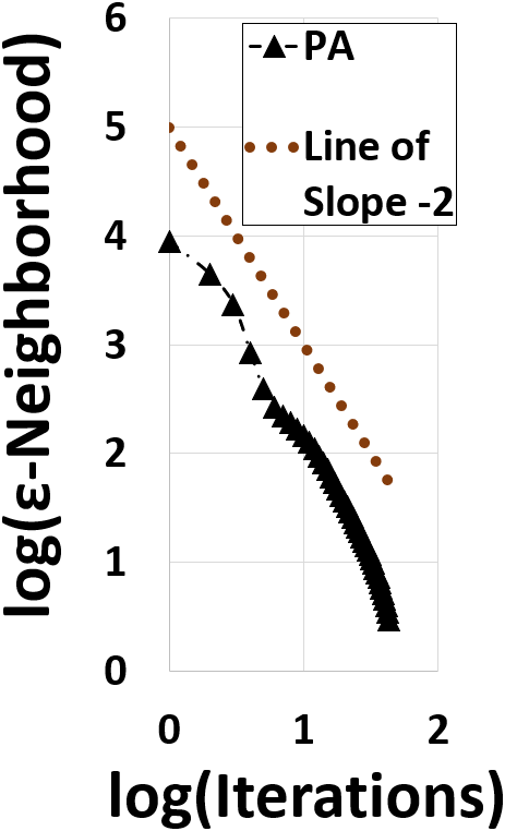
(a) Classification with $l_{2}$ norm.

(b) Matrix completion with Schatten-$2$ norm.

Figure 5: Convergence rate of PA on classification and matrix completion tasks.

In this section, we report experiments on various machine learning tasks and datasets to compare PA’s performance against other variants of FW when solving (smooth) convex functions with strongly convex constraint sets. In particular, we studied the performance of PA, FWLS, and FWPLR for both $l_{2}$ and Schatten-$2$ balls as our strongly convex constraint sets (see Section 3.1 for a discussion of why these constraints are strongly convex). We used the $l_{2}$ norm ball for a logistic classifier on the Adult dataset, as well as a linear regression task on the YearPredictionMSD dataset. We used the Schatten-$2$ norm ball for a matrix completion task on the MovieLens dataset.

First, we measured the $\epsilon$-neighborhood of the global minimum reached by PA at each iteration. Our theoretical results (Theorem 1) predict a convergence rate of $O(\frac{1}{t^{2}})$ in this case. To confirm this empirically, we plotted the logarithm of the $\epsilon$-neighborhood against the logarithm of the iteration number. If the convergence rate of $O(\frac{1}{t^{2}})$ were to hold, we would expect a straight line with a slope of $-2$ after taking the logarithms.

The plots are shown in Figures 5(a) and 5(b) for the classification and matrix completion tasks, respectively. The results confirm our theoretical results, as the plots exhibit a slope of -2.34 and -2.41, respectively. Note that a slightly steeper slope is expected in practice, since our theoretical results only provide a worst-case upper bound on the convergence rate.

B.4 Primal Averaging’s Performance versus Other FW Variants

(a) Regression with $l_{2}$ norm.

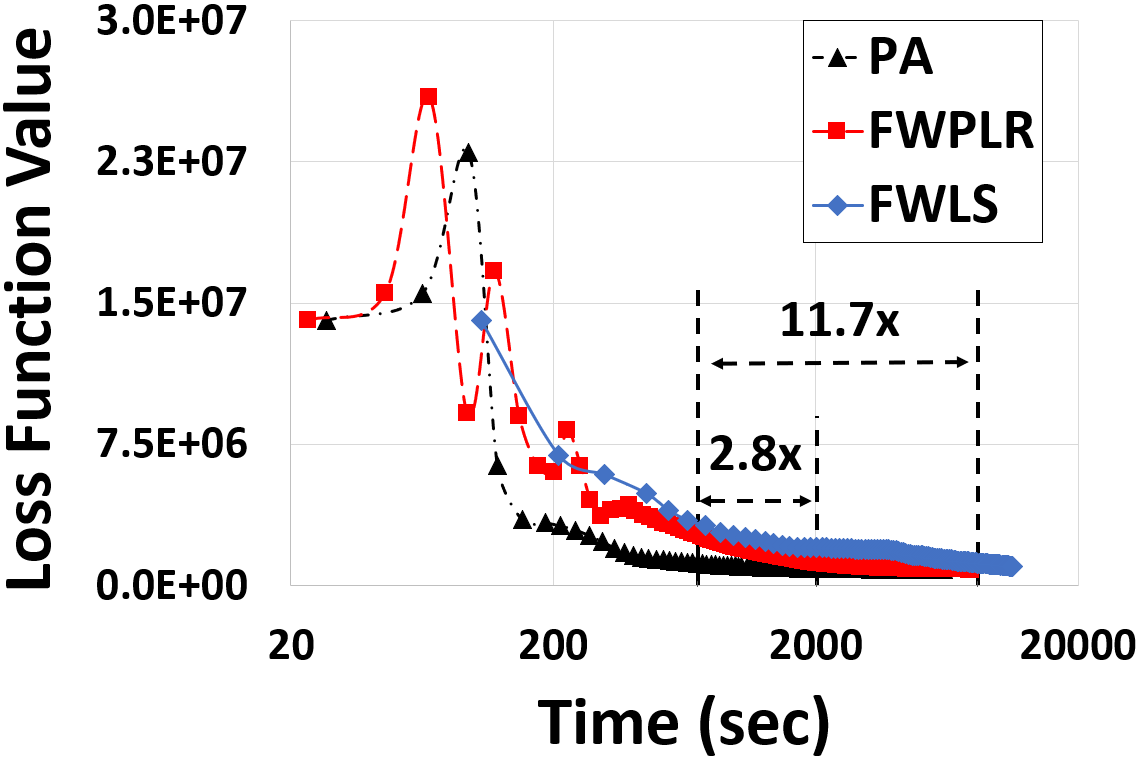
(b) Matrix completion with Schatten-$2$ norm.

Figure 6: Performance of different Frank-Wolfe variants on regression and matrix completion tasks.

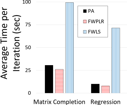
Figure 7: Average iteration time of PA, FWPLR, and FWLS on regression and matrix completion tasks.

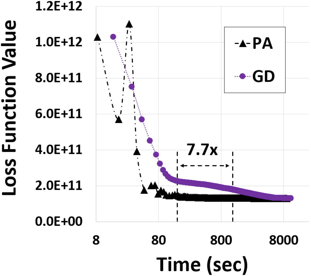
(a) PA versus GD.

(b) SPA versus SGD with $l_{2}$ norm.

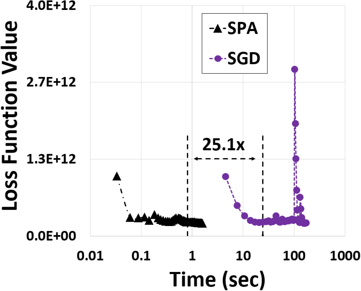
(c) SPA vs SGD with $l_{1.1}$ norm.

Figure 8: Performance of PA versus GD (and their stochastic versions, SPA and SGD) on the regression task.

To compare the actual performance of various FW variants on convex functions, we used the same settings as Section B.3. However, instead of the number of iterations to convergence, this time we measured the actual runtimes.

Here, we compared all three variants: PA, FWLS, and FWPLR. Figures 6(a) and 6(b) report the time taken to achieve each value of the loss function for the regression and matrix completion tasks, respectively. To compare the performance of these algorithms, we measured the difference between the time it took for each of them to converge. To determine convergence, here picked the first iteration at which the loss value was within $\pm 2\%$ of the previous loss value (practical convergence), and was also within $\pm 2\%$ of the global minimum (actual convergence). The first time at which these iterations were reached for each algorithm are marked by vertical, striped lines in Figures 6(a) and 6(b).

For the regression task, PA converged $3.7\times$ and $15.6\times$ faster than FWPLR and FWLS, respectively. For the matrix completion task, PA converged $2.8\times$ and $11.7\times$ faster than FWPLR and FWLS, respectively. These considerable speedups have significant ramifications in practice. Traditionally, PA has been shied away from, simply because it is slower in each iteration (due to PA’s use of auxiliary sequences and its extra summation step), while its convergence rate was believed to be the same as the more efficient variants (?). However, as we formally proved in Section 4, PA does indeed converge within much fewer iterations. Thus, the results shown in Figures 6(a) and 6(b) validate our hypothesis that PA’s faster convergence rate more than compensates for its additional computation at each iteration. Figure 7 reports the per-iteration cost of these FW variants on average, showing that PA is only 1.2–1.3x slower than than FWPLR in each iteration. This is why PA’s much faster convergence rate leads to much better performance in practice, compared to FWPLR. On the other hand, although FWLS offers the same convergence rate as PA, PA’s cost per iteration is $3.2$–$7.1\times$ faster than FWLS, which also explains PA’s superior performance over FWLS.

Finally, we note that PA’s improvements were much more drastic for the regression task than the matrix completion task ($3.7$–$15.6\times$ versus $2.8$–$11.7\times$). This is due to of the following reason. We recall that the Schatten-$p$ norm ball with radius $r$ is $\alpha$-strongly convex for $p\in(1,2]$ and with $\alpha=\frac{p-1}{r}$. The matrix completion task on the MovieLens dataset requires us to predict the values of a $6,040\times 3,900$ matrix ($6,040$ users and $3,900$ movies). Thus, to be able to maintain a reasonable number of potential matrices within our constraint set, we had to set $r=12000$, namely $\alpha=\frac{1}{12000}$. According to Theorem 1, the convergence rate is $O(\frac{L}{\alpha^{2}g^{2}t^{2}})$, which is why a small value of $\alpha$ slows down PA’s convergence.

B.5 Primal Averaging’s Performance versus Projected Gradient Descent

In this section, we compare the performance of PA and projected gradient descent. We evaluated deterministic and stochastic versions of both algorithms on the regression task with the same settings as in Section B.4. We used the same methodology to determine convergence as in Section B.4.

The results are shown in Figure 8. As expected, PA significantly outperformed projected GD, converging $7.7\times$ faster (Figure 8(a)). To better compare their stochastic versions (SPA and SGD), however, we used two different settings. The first used the $l_{2}$ ball as the constraint set, as an example of a case with an efficient projection, and the second used the $l_{1.1}$ ball as an example of a case with a costly projection.

The results conformed with our expectation again. When the projection onto the constraint set was efficient, SGD converged $4.6\times$ faster than SPA (Figure 2(c)). On the other hand, when the projection was costly, SPA far outperformed SGD, converging $25.1\times$ faster (Figure 8(c)).

B.6 Frank-Wolfe for (Smooth) Strictly-Locally-Quasi-Convex Functions

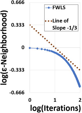
(a) Convergence rate when
$\epsilon<1$.

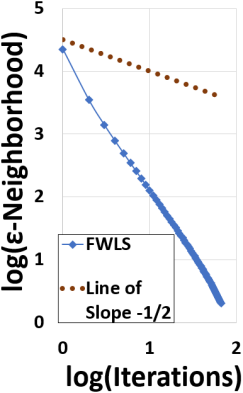
(b) Convergence rate when
$\epsilon>1$.

Figure 9: Iterations for FWLS to converge to an $\epsilon$-neighborhood when optimizing a strictly-locally-quasi-convex function.

According to Theorem 3, even when the loss function is not convex, FWLS still converges (to an $\epsilon$-neighborhood of the global minimum) within $O(max(\frac{1}{\epsilon^{2}},\frac{1}{\epsilon^{3}}))$ iterations, as long as the loss function is strictly-locally-quasi-convex. To verify this empiricially, we used the squared Sigmoid loss function for a classification task (Adult dataset) with an $l_{2}$ ball as our constraint set.

Note that, to conform with our theoretical result, FWLS must exhibit an $O\left(\frac{1}{t^{1/2}}\right)$ convergence rate when $\epsilon>1$ and an $O\left(\frac{1}{t^{1/3}}\right)$ convergence rate when $\epsilon<1$. To better illustrate this difference, we examine two plots: Figure 9(b) displays the iterations where $\epsilon>1$, while Figure 9(a) displays the iteration where $\epsilon<1$. Both plots show the logarithm of the $\epsilon$-neighborhood against the logarithm of the iteration number. This means we should expect to see the loss values decreasing at a slope steeper than or equal to $-\frac{1}{2}$ and $-\frac{1}{3}$ in Figure 9(b) and Figure 9(a), respectively.

The plots confirm our theoretical results, exhibiting a slope of $-2.12$ when $\epsilon>1$ and $-0.377$ when $\epsilon<1$. Note that the steeper slopes here are expected, as our theoretical results only provide a worst-case upper bound on the convergence rate. Notably, FWLS showed a significantly steeper slope when $\epsilon>1$. We observe that the convergence rate bound for $\epsilon>1$ is missing the smoothness parameter $L$ of the $\epsilon<1$ bound. It is noted in (?) that using the squared Sigmoid loss is equivalent to the perceptron problem with a $\gamma$-margin, and Kalai and Sastry (?) show that the smoothness parameter $L$ of the latter is $\frac{1}{\gamma}$. Thus, when the margin is large, the $\epsilon<1$ case is able to converge at a rate closer to $O\left(\frac{1}{t^{1/3}}\right)$ than the $\epsilon>1$ case to its rate of $O\left(\frac{1}{t^{1/2}}\right)$. Thus, we hypothesize that it is the absence of the $L$ factor in the upper bound for $\epsilon>1$, which primarily contributes to its convergence rate being faster than $-\frac{1}{2}$ when $\epsilon>1$.

Figure 10: Performance of FWLS for regression with a non-convex loss.

B.7 Frank-Wolfe for (Smooth) Non-Convex Functions

In Theorem 4, we proved that FWLS converges to a stationary point of (smooth) non-convex functions at a rate of $O(\frac{1}{t})$, as long as it is constrained to a strongly convex set. To empirically verify whether this upper bound is tight, we use the bi-weight loss (see Section B.1 and Table 3) in a classification task (Adult dataset) with an $l_{2}$ ball constraint.

In Figure 10, we measured the $\epsilon$-neighborhood reached by FWLS at each iteration, plotting the logarithm of the $\epsilon$-neighborhood against the logarithm of the iteration number. To confirm the $O(\frac{1}{t})$ convergence rate found in Theorem 4, we expect to see a straight line of slope $-1$ in Figure 10.

The empirical results confirm our theoretical results, showing a slope of $-1.46$. Again, we note that a steeper slope is expected in practice as Theorem 4 only provides a worst-case upper bound on the convergence rate.

References

- [Agarwal et al. 2017] Agarwal, N.; Allen-Zhu, Z.; Bullins, B.; Hazan, E.; and Ma, T. 2017. Finding approximate local minima for nonconvex optimization in linear time. STOC.
- [Agarwal, Negahban, and Wainwright 2010] Agarwal, A.; Negahban, S.; and Wainwright, M. J. 2010. Fast global convergence rates of gradient methods for high-dimensional statistical recovery. In Advances in Neural Information Processing Systems, 37–45.
- [Beck and Teboulle 2004] Beck, A., and Teboulle, M. 2004. A conditional gradient method with linear rate of convergence for solving convex linear systems. Mathematical Methods of Operations Research 59(2):235–247.
- [Belagiannis et al. 2015] Belagiannis, V.; Rupprecht, C.; Carneiro, G.; and Navab, N. 2015. Robust optimization for deep regression. In Proceedings of the IEEE International Conference on Computer Vision, 2830–2838.
- [Buja, Stuetzle, and Shen 2005] Buja, A.; Stuetzle, W.; and Shen, Y. 2005. Loss functions for binary class probability estimation and classification: Structure and applications. Working draft, November.
- [Candès and Recht 2009] Candès, E. J., and Recht, B. 2009. Exact matrix completion via convex optimization. Foundations of Computational mathematics 9(6):717.
- [Carmon et al. 2017] Carmon, Y.; Duchi, J.; Hinder, O.; and Sidford, A. 2017. Accelerated methods for non-convex optimization. https://arxiv.org/pdf/1611.00756.pdf.
- [Chari et al. 2015] Chari, V.; Lacoste-Julien, S.; Laptev, I.; and Sivic, J. 2015. On pairwise costs for network flow multi-object tracking. CVPR.
- [Clarkson 2010] Clarkson, K. L. 2010. Coresets, sparse greedy approximation, and the frank-wolfe algorithm. ACM Transactions on Algorithms (TALG) 6(4):63.
- [Demyanov and Rubinov 1970] Demyanov, V. F., and Rubinov, A. M. 1970. Approximate methods in optimization problems. Elsevier Publishing Company,.
- [Dunn 1979] Dunn, J. C. 1979. Rates of convergence for conditional gradient algorithms near singular and nonsingular extremals. SIAM Journal on Control and Optimization.
- [Frank and Wolfe 1956] Frank, M., and Wolfe, P. 1956. An algorithm for quadratic programming. Naval research logistics quarterly 3(1-2):95–110.
- [Freund, Grigas, and Mazumder 2017] Freund, R. M.; Grigas, P.; and Mazumder, R. 2017. An extended frank–wolfe method with “in-face” directions, and its application to low-rank matrix completion. SIAM Journal on Optimization 27(1):319–346.
- [Garber and Hazan 2015] Garber, D., and Hazan, E. 2015. Faster rates for the frank-wolfe method over strongly-convex sets. In International Conference on Machine Learning, 541–549.
- [Ge et al. 2015] Ge, R.; Huang, F.; Jin, C.; and Yuan, Y. 2015. Escaping from saddle points – online stochastic gradient for tensor decomposition. COLT.
- [Ghadimi and Lan 2016] Ghadimi, S., and Lan, G. 2016. Accelerated gradient methods for nonconvex nonlinear and stochastic programming. Mathematical Programming 156(1-2):59–99.
- [Grant and Boyd ] Grant, M., and Boyd, S. Cvx: Matlab software for disciplined convex programming.
- [Grant and Boyd 2008] Grant, M. C., and Boyd, S. P. 2008. Graph implementations for nonsmooth convex programs. In Recent advances in learning and control. Springer. 95–110.
- [Harchaoui et al. 2012] Harchaoui, Z.; Douze, M.; Paulin, M.; Dudik, M.; and Malick, J. 2012. Large-scale image classification with trace-norm regularization. In Computer Vision and Pattern Recognition (CVPR), 2012 IEEE Conference on, 3386–3393. IEEE.
- [Harper and Konstan 2016] Harper, F. M., and Konstan, J. A. 2016. The movielens datasets: History and context. ACM Transactions on Interactive Intelligent Systems (TiiS) 5(4):19.
- [Hazan and Kale 2012] Hazan, E., and Kale, S. 2012. Projection-free online learning. arXiv preprint arXiv:1206.4657.
- [Hazan and others 2016] Hazan, E., et al. 2016. Introduction to online convex optimization. Foundations and Trends® in Optimization 2(3-4):157–325.
- [Hazan, Kale, and Warmuth 2010] Hazan, E.; Kale, S.; and Warmuth, M. K. 2010. Learning rotations with little regret. In COLT, 144–154.
- [Hazan, Levy, and Shalev-Shwartz 2015] Hazan, E.; Levy, K. Y.; and Shalev-Shwartz, S. 2015. Beyond convexity: Stochastic quasi-convex optimization. Neural Information Processing Systems.
- [Huang and Chen 2011] Huang, W., and Chen, D.-R. 2011. Gradient iteration with lp-norm constraints. Journal of Mathematical Analysis and Applications.
- [Huang et al. 2016] Huang, R.; Lattimore, T.; György, A.; and Szepesvari, C. 2016. Following the leader and fast rates in linear prediction: Curved constraint sets and other regularities.
- [Jaggi, Sulovsk, and others 2010] Jaggi, M.; Sulovsk, M.; et al. 2010. A simple algorithm for nuclear norm regularized problems. In Proceedings of the 27th international conference on machine learning (ICML-10), 471–478.
- [Jaggi 2011] Jaggi, M. 2011. Sparse convex optimization methods for machine learning. Technical report, ETH Zürich.
- [Jaggi 2013] Jaggi, M. 2013. Revisiting frank-wolfe: Projection-free sparse convex optimization. In ICML (1), 427–435.
- [Kalai and Sastry 2009] Kalai, A. T., and Sastry, R. 2009. The isotron algorithm: High-dimensional isotonic regression. In COLT.
- [Kim and Xing 2010] Kim, S., and Xing, E. P. 2010. Tree-guided group lasso for multi-task regression with structured sparsity.
- [Koltchinskii et al. 2011] Koltchinskii, V.; Lounici, K.; Tsybakov, A. B.; et al. 2011. Nuclear-norm penalization and optimal rates for noisy low-rank matrix completion. The Annals of Statistics 39(5):2302–2329.
- [Lacoste-Julien and Jaggi 2015] Lacoste-Julien, S., and Jaggi, M. 2015. On the global linear convergence of frank-wolfe optimization variants. In Advances in Neural Information Processing Systems, 496–504.
- [Lacoste-Julien et al. 2013] Lacoste-Julien, S.; Jaggi, M.; Schmidt, M.; and Pletscher, P. 2013. Block-coordinate frank-wolfe optimization for structural svms. ICML.
- [Lacoste-Julien 2016] Lacoste-Julien, S. 2016. Convergence rate of frank-wolfe for non-convex objectives,. arXiv:1607.00345.
- [Lan 2013] Lan, G. 2013. The complexity of large-scale convex programming under a linear optimization oracle. https://arxiv.org/abs/1309.5550.
- [Lee et al. 2016] Lee, J. D.; Simchowitz, M.; Jordan, M. I.; and Recht, B. 2016. Gradient descent converges to minimizers. COLT.
- [Levitin and Polyak 1966] Levitin, E. S., and Polyak, B. T. 1966. Constrained minimization methods. USSR Computational mathematics and mathematical physics.
- [Lichman 2013] Lichman, M. 2013. UCI machine learning repository.
- [Liu et al. 2015] Liu, J.; Wright, S. J.; Ré, C.; Bittorf, V.; and Sridhar, S. 2015. An asynchronous parallel stochastic coordinate descent algorithm. The Journal of Machine Learning Research 16(1):285–322.
- [Nesterov and Polyak 2006] Nesterov, Y., and Polyak, B. T. 2006. Cubic regularization of newton method and its global performance. Mathematical Programming 108(1):177–205.
- [Neter et al. 1996] Neter, J.; Kutner, M. H.; Nachtsheim, C. J.; and Wasserman, W. 1996. Applied linear statistical models, volume 4. Irwin Chicago.
- [Osokin et al. 2016] Osokin, A.; Alayrac, J.-B.; Lukasewitz, I.; Dokania, P.; and Lacoste-Julien, S. 2016. Minding the gaps for block frank-wolfe optimization of structured svms. In International Conference on Machine Learning, 593–602.
- [Park et al. 2018] Park, Y.; Qing, J.; Shen, X.; and Mozafari, B. 2018. BlinkML: Approximate machine learning with probabilistic guarantees y. Technical Report http://web.eecs.umich.edu/~mozafari/php/data/uploads/blinkml_report.pdf.
- [Recht and Ré 2013] Recht, B., and Ré, C. 2013. Parallel stochastic gradient algorithms for large-scale matrix completion. Mathematical Programming Computation 5(2):201–226.
- [Recht et al. 2011] Recht, B.; Re, C.; Wright, S.; and Niu, F. 2011. Hogwild: A lock-free approach to parallelizing stochastic gradient descent. In Advances in neural information processing systems, 693–701.
- [Reddi et al. 2016] Reddi, S. J.; Sra, S.; Poczos, B.; and Smola., A. 2016. Stochastic frank-wolfe methods for nonconvex optimization. Allerton.
- [Shalev-Shwartz, Gonen, and Shamir 2011] Shalev-Shwartz, S.; Gonen, A.; and Shamir, O. 2011. Large-scale convex minimization with a low-rank constraint. arXiv preprint arXiv:1106.1622.
- [Sun and Yuan 2006] Sun, W., and Yuan, Y.-X. 2006. Optimization theory and methods: nonlinear programming, volume 1. Springer Science & Business Media.
- [Wang et al. 2016] Wang, Y.-X.; Sadhanala, V.; Dai, W.; Neiswanger, W.; Sra, S.; and Xing, E. 2016. Parallel and distributed block-coordinate frank-wolfe algorithms. In International Conference on Machine Learning, 1548–1557.
- [Yu, Zhang, and Schuurmans 2014] Yu, Y.; Zhang, X.; and Schuurmans, D. 2014. Generalized conditional gradient for structured estimation. arXiv:1410.4828.