Interstellar Medium and Star Formation of Starburst Galaxies on the Merger Sequence

Abstract

The interstellar medium is a key ingredient that governs star formation in galaxies. We present a detailed study of the infrared ($\sim 1-500$ µm) spectral energy distributions of a large sample of 193 nearby ($z\lesssim 0.088$) luminous infrared galaxies (LIRGs) covering a wide range of evolutionary stages along the merger sequence. The entire sample has been observed uniformly by 2MASS, WISE, Spitzer, and Herschel. We perform multi-component decomposition of the spectra to derive physical parameters of the interstellar medium, including the intensity of the interstellar radiation field and the mass and luminosity of the dust. We also constrain the presence and strength of nuclear dust heated by active galactic nuclei. The radiation field of LIRGs tends to have much higher intensity than in quiescent galaxies, and it increases toward advanced merger stages as a result of central concentration of the interstellar medium and star formation. The total gas mass is derived from the dust mass and the galaxy stellar mass. We find that the gas fraction of LIRGs is on average $\sim$0.3 dex higher than that of main-sequence star-forming galaxies, rising moderately toward advanced merger stages. All LIRGs have star formation rates that place them above the galaxy star formation main sequence. Consistent with recent observations and numerical simulations, the global star formation efficiency of the sample spans a wide range, filling the gap between normal star-forming galaxies and extreme starburst systems.

1 Introduction

Luminous infrared galaxies (LIRGs; Sanders & Mirabel 1996), defined as systems with total infrared (IR; 8–1000 µm) luminosity $L_{\mathrm{IR}}$ $>10^{11}\,L_{\odot}$, have been studied extensively since they were recognized as a major constituent of the galaxy population from the Infrared Astronomical Satellite (IRAS) all-sky survey. The power source of the IR emission, whether it be star formation and/or active galactic nuclei (AGNs), has been intensively debated over the years (e.g., Genzel et al. 1998; Lutz et al. 1998; Spoon et al. 2007; Veilleux et al. 2009; Yuan et al. 2010; Iwasawa et al. 2011; Petric et al. 2011). The star formation rate (SFR) of LIRGs, inferred from IR luminosity, generally exceeds $\gtrsim 10$ $M_{\odot}\>\mathrm{yr^{-1}}$, qualifying them as starburst systems that lie above the SFR–$M_{*}$ “main sequence” relation of low-$z$ star-forming galaxies (e.g., Daddi et al. 2007; Noeske et al. 2007; Peng et al. 2010; Renzini & Peng 2015). Moreover, LIRGs dominate star formation at $z\gtrsim 1$ (e.g., Elbaz et al. 2002; Chapman et al. 2005). Nearby LIRGs that are well-measured at a wide variety of wavelengths are, therefore, important to shed light on galaxy star formation at high redshifts. Given their state of rapid stellar mass growth, LIRGs are important to study the coevolution of galaxies and their central supermassive black holes (Kormendy & Ho 2013). The most luminous members of the class—ULIRGs—may evolve into quasars (Sanders et al. 1988a, 1988b) and, finally, massive elliptical galaxies (Wright et al. 1990; Genzel et al. 2001; Tacconi et al. 2002) with the aid of AGN feedback (Di Matteo et al. 2005; Hopkins et al. 2008; but see Shangguan et al. 2018, and references therein).

The interstellar medium (ISM) is of great importance to understand the physics of star formation in LIRGs. Early CO observations (e.g., Sanders & Mirabel 1985; Sanders et al. 1986, 1991; Young et al. 1986) revealed that LIRGs contain large amounts of molecular gas, but that they emit IR emission in excess of the $L^{\prime}_{\mathrm{CO}}$–$L_{\mathrm{IR}}$ relation of normal, star-forming galaxies. Interferometric observations of some small samples of LIRGs with signatures of interactions found the CO emission mostly concentrated in the central regions (Downes & Solomon 1998; Bryant & Scoville 1999). More recent, high-resolution observations show that the molecular gas in LIRGs is concentrated in compact central disks associated with nuclear starbursts (Ueda et al. 2014; Xu et al. 2014, 2015; Scoville et al. 2015). It has been widely debated whether starburst systems follow the same relation between SFR and gas content as regular, star-forming galaxies. Kennicutt (1998a) argues that normal galaxies, starburst nuclei, and LIRGs obey the same empirical relation between SFR surface density and total gas (H I+H₂) mass surface density. However, more recent CO surveys suggest that normal galaxies and starburst systems behave differently in terms of their relation between the molecular gas and SFR (Daddi et al. 2010; Genzel et al. 2010), with the caveat that the conversion factor from CO emission to molecular gas mass (Bolatto et al. 2013) remains controversial (e.g., Liu et al. 2015).

From a theoretical point of view, mergers and interactions are expected to efficiently drive gas inflow toward the galactic center, igniting a central starburst (e.g., Barnes & Hernquist 1996; Mihos & Hernquist 1996; Bournaud et al. 2011; Hopkins et al. 2013). However, the gas kinematics in mergers are complex and comparison with model predictions is not straightforward (Iono et al. 2004a, 2005; Saito et al. 2015). In the local Universe ($z\lesssim 0.1$), the Great Observatories All-sky LIRG Survey (GOALS; Armus et al. 2009) provides a complete sample of 201 LIRGs with observations from radio to X-rays. This sample of IR-luminous galaxies span a diverse range of morphologies: non-mergers, pre-mergers, and mergers from early to late stage (Haan et al. 2011; Petric et al. 2011; Stierwalt et al. 2013; Larson et al. 2016). Objects with the highest IR luminosities are primarily late-stage mergers (Sanders 1988a; Dinh-V-Trung et al. 2001; Veilleux et al. 2002; Kim et al. 2013). The diversity of merger stages encapsulated in GOALS is important to reveal the properties of the gas content along the evolutionary merger sequence. Yamashita et al. (2017) recently show that the size of the CO emission in the central kpc decreases from early- to late-stage mergers, while the molecular gas mass remains constant, statistically supporting the notion that gas inflow commonly replenishes nuclear starbursts in merging LIRGs.

We combine 2MASS, WISE, and Herschel photometric measurements to analyze the IR (1–500 µm) spectral energy distributions (SEDs) of the entire GOALS sample. We derive the mass and luminosity of the dust associated with the large-scale ISM of the host galaxy, after decomposing the emission from the hot dust powered by the AGN, and we place constraints on the intensity of the interstellar radiation field (ISRF). The total gas mass and the SFR are then derived. LIRGs tend to have moderately higher ISM fractions than normal, star-forming galaxies, possibly due to selection effects. The large sample size and diverse morphologies of GOALS enables us to compare the distribution of physical properties as a function of different merger stages. We find that the ISRF intensity, as probed by the galactic dust, increases toward the advanced merger stages, as does the ISM mass fraction. LIRGs occupy a wide region above the main sequence of low-$z$ star-forming galaxies, with late-stage mergers exhibiting the highest SFRs. The star formation efficiency (SFE), although spanning a wide range across the sample, tends to increase toward advanced merger stages. LIRGs fills the bimodality of SFE previously found for normal and starburst systems.

This paper is organized as follows. Section 2 describes the details of the sample and the data reduction. We explain the methods to model the SEDs in Section 3 and present the SED fitting results in Section 4. The stellar mass and ISM properties are presented in Section 5. Section 6 discusses star formation in LIRGs. We summarize the main conclusions in Section 7. This work adopts the following parameters for a $\Lambda$CDM cosmology: $\Omega_{m}=0.308$, $\Omega_{\Lambda}=0.692$, and $H_{0}=67.8$ km s^-1 Mpc^-1 (Planck Collaboration et al. 2016).

2 Sample & data reduction

The 201 LIRGs from the GOALS sample are all mapped by the Herschel Space Observatory (Pilbratt et al. 2010) with both the Photodetector Array Camera and Spectrometer (PACS; Poglitsch et al. 2010), at 70, 100, and 160 µm, and the Spectral and Photometric Imaging Receiver (SPIRE; Griffin et al. 2010), at 250, 350, and 500 µm. Most of the merger systems are covered by single maps with each instrument. Meanwhile, eight systems consist of widely separated pairs that require two PACS maps; their two components are measured separately. Chu et al. (2017) provide integrated aperture photometry of the Herschel data for the entire GOALS sample. We use their measurements of total integrated flux for the PACS and SPIRE data for all the 201 systems. We supplement these data with our own measurements of near-IR photometry from 2MASS (Skrutskie et al. 2006) and mid-IR photometry from WISE (Wright et al. 2010) to construct the full IR SED from 1 to 500 µm.

We download the 2MASS and WISE images from the NASA/IPAC Infrared Science Archive (IRSA) and uniformly measure the integrated aperture photometry for the entire systems. The details of our method, presented by Li et al. (2018, in preparation), are briefly summarized here. A source mask is generated for each image based on the image segmentation file. The sky background of the image is fitted with a third-order polynomial function and subtracted; this suffices to remove the large-scale gradient in all of the 2MASS and WISE images. We measure the surface brightness profile of the targets by fitting isophotes with the IRAF task ellipse. The aperture in each band is determined separately by the isophote whose surface brightness reaches the large-scale variation of the background, which is estimated by sampling the rebinned background pixels. One large aperture is used to enclose the entire merger system if the two galaxies are not coalesced, as we usually lack the resolution to separate the two galaxies in Herschel maps. In order to provide aperture photometry consistent throughout the various IR bands, we choose the largest semi-major axis and semi-minor axis among all of the bands to arrive at the final aperture applicable to all the 2MASS and WISE images for each object. The final aperture sizes are always larger than the aperture adopted by Chu et al. for their Herschel measurements. We omit five objects that are too large to be fully covered by 2MASS and three objects contaminated by bright stars, mostly in $W$1 and $W$2, resulting in the final sample of 193 LIRGs used in our current study.

Shangguan et al. (2018) showed that even SEDs that contain only photometric data from 2MASS, WISE, and Herschel can still yield robust cold dust masses and far-IR luminosities for the host galaxies of type 1 quasars. However, the situation for some LIRGs is more complicated because of the strong effect of silicate absorption features, which cannot be constrained well with photometric data alone. While Spitzer/IRS data exist for all GOALS objects, many of spectra cannot be directly used in the SED fitting because of their limited slit coverage. Using a subset of 61 objects with IRS spectra that reasonably match the photometric data (Appendix A), we show, by comparison of fits with and without inclusion of the spectra that the photometric SEDs alone can measure the interesting physical parameters without significant bias (Appendix B).

Table 1 lists the basic information and the physical results from our photometric SED analysis of the sample of 193 LIRGs. The luminosity distance is derived by correcting the heliocentric velocity from the galaxy peculiar motion using the 3-attractor flow model of Mould et al. (2000) and adopting our current cosmology for consistency. We adopt the visually derived merger stage classification of Stierwalt et al. (2013), which is mainly based on Spitzer/IRAC 3.6 µm images ($\sim$ 2″ resolution) but complemented, whenever available, by high-resolution images from the Hubble Space Telescope (Haan et al. 2011). They categorize the morphologies into five types: “n” for non-mergers (no signs of merger activity or massive neighbors), “a” for pre-mergers (galaxy pairs prior to a first encounter), “b” for early-stage mergers (post-first-encounter with galaxy disks still symmetric but with signs of tidal tails), “c” for mid-stage mergers (showing amorphous disks, tidal tails, and other signs of merger activity), and “d” for late-stage mergers (two nuclei in a common envelope). With additional ground-based optical images, Larson et al. (2016) compare their visual classifications to those of Stierwalt et al. (2013) for 65 objects in common and find reasonable consistency. Due to limitations in resolution and sensitivity, stage “b” objects have a $\sim 50\%$ chance of being confused with stage “a” or “c”; stage “d” sources have $\lesssim 50\%$ chance of confusion with stage “c” and almost none with stage “n”. This level of uncertainty is, in fact, adequate for our purposes.

3 SED models

The SED fitting is conducted with a Bayesian Markov Chain Monte Carlo (MCMC) method developed by Shangguan et al. (2018). The IR SED of a galaxy is dominated by stellar emission in the near-IR and dust emission at longer wavelengths. We model the stellar emission as a 5 Gyr simple stellar population (Bruzual & Charlot 2003; BC03), adopting a Chabrier (2003) initial mass function (IMF) and solar metallicity. As the near-IR spectral shape of stellar emission is mostly governed by the old stellar population, it is relatively insensitive to stellar age. Therefore, fixing the stellar age of the BC03 model will barely affect the SED fitting at longer wavelengths. Nuclear activity can produce prominent hot dust emission in the mid-IR, which can be modeled as a dusty torus. We fit the cold dust emission from the host galaxy with the widely used physical dust model from Draine & Li (2007; DL07), which is based on the dust composition and size distribution observed in the Milky Way. Two components of dust are considered: (1) most of the dust mass usually resides in the “diffuse” ISM exposed to the galactic ISRF with a minimum intensity $U=U_{\mathrm{min}}$; (2) a smaller mass fraction ($\gamma$) of the dust is associated with “photo-dissociation regions” heated by the ISRF with a power-law intensity distribution $U_{\mathrm{min}}<U<U_{\mathrm{max}}$. The power-law index is fixed to $\alpha=2$, and the maximum field intensity is set to $U_{\mathrm{max}}=10^{6}$ (Draine et al. 2007). The mass fraction of nanometer-size dust, a mixture of amorphous silicate and graphite, including polycyclic aromatic hydrocarbons (PAHs), is parameterized as $q_{\mathrm{PAH}}$.

For the objects that require a torus component, we adopt a new version of the CAT3D model (Hönig & Kishimoto 2017) to fit the AGN dust torus emission. This model considers the different sublimation temperatures of silicate and graphite dust, self-consistently providing more emission from the hot dust at the inner edge of the torus, which was lacking in previous models such as CLUMPY (Nenkova et al. 2008a, 2008b), as well as in the earlier version of CAT3D (Hönig & Kishimoto 2010). Motivated by interferometric observations (e.g., Raban et al. 2009), the new model can also include a wind component, which allows greater flexibility to accommodate the diversity of IR SEDs of quasars (Zhuang et al. 2018). The basic CAT3D torus model consists five parameters: the inclination angle, $i$; the power-law index $a$ of the cloud radial distribution, of the form $r^{a}$, with $r$ the distance from the center in units of the sublimation radius $r_{\mathrm{sub}}$; the dimensionless scale height $h$ of the Gaussian distribution of clouds in the vertical direction, of the form $\exp\{-z^{2}/2(hr)^{2}\}$, with $z$ the vertical distance from the mid-plane; the average number $N_{0}$ of clouds along the equatorial line-of-sight; and the normalization factor $L$. Limited by the degree of freedom, we use the basic CAT3D model to fit the photometric SEDs. The fits that incorporate IRS spectra (Appendix B) are conducted with an additional wind component, which adds four additional free parameters: the radial distribution $a_{w}$ of dust clouds, the half-opening angle $\theta_{w}$, the angular width $\sigma_{\theta}$, and the wind-to-disk ratio $f_{\rm wd}$, which defines the ratio of the number of clouds along the cone and $N_{0}$. García-González et al. (2017) also recently provide a new set of torus templates based on the CAT3D model. We find that the choice of the torus model has little, if any, effect on measurements of cold dust properties. Specifically, our various tests (see Appendix B; Shangguan et al. 2018; Zhuang et al. 2018; Shangguan & Ho 2018) find that the dust mass and $U_{\mathrm{min}}$ show scatter less than 0.1 and 0.15 dex without significant systematic deviation. We choose to use the results based on the templates from Hönig et al. (2017), as they provide the best overall fits (Zhuang et al. 2018).

The silicate absorption at 9.7 µm and 18 µm in Spitzer/IRS spectra indicates significant mid-IR extinction for a considerable fraction of our sample. It is important to properly take into account dust extinction, as it affects not only the silicate features but also the overall shape of the broad-band continuum. We adopt the dust extinction model of Smith et al. (2007). The extinction model consists of a power law plus silicate features peaking at 9.7 and 18 $\mu$m, using the absorption properties of dust measured from the Milky Way. Because the original extinction curve of Smith et al. (2007) ends at $\sim 38$ µm, we extrapolate the curve to 1000 $\mu$m with a Drude profile with $\gamma_{r}=0.247$ peaking at 18 µm, assuming no additional extinction features beyond 38 µm (Mathis et al. 1990). The only free parameter for the mid-IR extinction model is $\tau_{9.7}$, the optical depth at 9.7 µm.

4 SED fitting

With the models in hand, a key problem is whether the fits should include a torus component. For most of the objects with relatively strong AGN-heated dust emission, models without a torus component cannot fit the data. However, most LIRGs have little if any obvious torus emission. While many of the GOALS objects have been previously studied in terms of their nuclear activity using a variety of multiwavelength diagnostics (e.g., Veilleux et al. 1999; Yuan et al. 2010; Iwasawa et al. 2011; Petric et al. 2011; Torres-Albà et al. 2018), their AGN classification is not always clear because of complications from dust obscuration, strong star formation activity, and complex gas kinematics. The mid-IR SED, on the other hand, is sensitive to the presence of the AGN dust torus (e.g., Stern et al. 2012; Blecha et al. 2018), such that highly obscured objects classified as non-AGNs by other methods may still show significant torus emission in the mid-IR (e.g., F00344$-$3349 and F01173+1405). In this study, we objectively ascertain whether a torus contribution is warranted based purely on the fitting results, not on any prior knowledge from other diagnostics. We fit the SEDs using models with and without a torus component and only choose the model with a torus component when the fit is significantly improved. Details of the fitting methods are reported in Section 4.1. In order to avoid model degeneracy, when the torus component is added, we fix $\gamma$ and $q_{\mathrm{PAH}}$ of the DL07 component. Thus, the fit is not always improved when the torus component is included. In order to determine the best-fit model objectively, we calculate a local $\chi^{2}$ for the mid-IR region, using only the $W$1 to $W$4 bands. Through various experimentation, we find that the torus component can be considered significant if including it in the fit reduces $\chi^{2}$ by more than a factor of 5. We visually inspect every fit and in the end conclude that 69 (36%) objects in the sample require a torus component. Among these, it is noteworthy that 42 have been diagnosed previously as AGNs in the literature (Table 1), while two-thirds of the remaining 27 objects are likely AGNs according to their WISE color ($W1-W2>0.5$; Mingo et al. 2016; Blecha et al. 2018). We attempt to quantify the presence of a torus merely for the sake of completeness. We emphasize that, as discussed in Shangguan et al. (2018), the properties of the cold dust derived from the DL07 component (e.g., $M_{d}$ and $U_{\mathrm{min}}$) are actually very insensitive to whether or how the torus component is included in the fit. Moreover, we find that the dust masses derived from full SED fitting are consistent with those obtained from fitting a modified blackbody (MBB) model to the FIR data only (Appendix D).

The mid-IR spectra of most of the sample only probe a fraction of the host galaxy due to the limited size of the IRS slit. Using a subsample of 61 objects whose IRS spectra are least affected by the problem of aperture mismatch, we show that the physical parameters of the DL07 model can be robustly derived from the photometric SED alone (Appendix B). Most of the objects that show significant deviation between the photometric and full SED fitting can be identified from careful visual inspection of the photometric fits. The unreliable fits usually show large, obvious mismatchs with the data or strong silicate absorption features, indicating that the model is poorly constrained by the data.

4.1 Fitting the photometric SED

We fit the SEDs using models with and without the torus component for all 193 objects with robust near-IR to far-IR photometric measurements. For fits without the torus component, we combine BC03 and DL07 components with the extinction applied to the latter. The DL07 parameters $q_{\mathrm{PAH}}$, $\gamma$, $U_{\mathrm{min}}$, and dust mass are all free. When the torus component is included, we combine BC03, CAT3D, and DL07 components, again with extinction excluded from the stellar emission. In view of the large number of free parameters and the very limited number of WISE photometric data points, it is necessary to make some simplifying assumptions and keep certain parameters fixed. We choose to use the CAT3D templates without the wind component, and for the DL07 component with $q_{\mathrm{PAH}}=0.47$ and $\gamma=0.03$, which are fiducial values found effective by Shangguan & Ho (2018) for type 2 quasars. The model parameters are summarized in Table 2.

In the fitting process, the model SED is multiplied by the filter transmission curve and integrated to calculate the average flux density of the various bands (see Shangguan et al. 2018 for more details). A considerable fraction of our targets are (marginally) extended even in the Herschel/SPIRE bands. The beam size of the SPIRE bands varies with frequency, and the relative spectral response function (RSRF) effectively changes from point sources to extended sources. Therefore, we need to evaluate the effect of the RSRF on our best-fit parameters of the DL07 component, namely $U_{\mathrm{min}}$ and dust mass. We select 30 objects that are mostly extended in SPIRE bands and fit their SEDs using the transmission curves for extended source. Comparing to fits with the transmission curves of point sources, the dust mass and $U_{\mathrm{min}}$ are affected only at the level of $\sim$0.05 dex, with no obvious systematics. Henceforth, we simply adopt the point-source RSRF.

Four examples of SED fits are shown in Figure 1, representing cases with low and high extinction, and low to moderate AGN torus contribution. For cases like 05368+4940 (Figure 1a), which does not require a torus, the fit is very good. In fact, the fits are generally robust even when the torus emission (Figure 1b) and/or the extinction (Figure 1c) is significant. However, the extinction cannot be accurately constrained when it is very strong, and the best-fit $U_{\mathrm{min}}$ and dust mass may not be reliable. Another problem is that the parameter range of $U_{\mathrm{min}}$ is limited to $\leq 25$, which is likely not high enough to fit some objects like F08572$+$3915. As shown in Figure 8d, the best-fit model still lies below the 70 and 100 µm data, such that in the photometric fit (Figure 1d) the torus component becomes very strong to compensate for the mismatch. We visually check all the photometric SED fits and only find complications in 13 (7%) of the cases; these are flagged in Table 1. All objects whose photometric SED fits significantly deviated from the more robust fits using the IRS spectra (Appendix B) are successfully identified by our visual inspection.

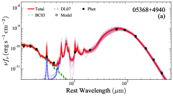
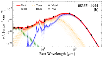
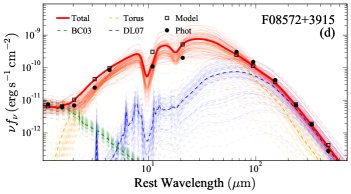
Figure 1: Examples of photometric SED fitting. The black points are the photometric data from 2MASS, WISE, and Herschel. The open squares are the model synthetic fluxes that can be directly compared with the data. The dashed lines are the individual components for stars (green; BC03), torus (orange; CAT3D), and host galaxy dust (blue; DL07). The combined best-fit model is plotted as a red solid line. To visualize the model uncertainties, the associated faint and thin lines represent 100 sets of models with parameters drawn randomly from the space sampled by the MCMC algorithm.

5 Results

5.1 Stellar mass

The stellar mass is derived from the $J$-band photometry with a mass-to-light ratio ($M/L$) constrained by the $B-I$ color (Bell & de Jong 2001):

$$\mathrm{log}\,(M_{*}/M_{\odot})=-0.4(M_{J}-M_{J,\odot})-0.75+0.34(B-I),$$ (1)

where $M_{J}$ and $M_{J,\odot}=3.65$ (Blanton & Roweis 2007) are the rest-frame $J$-band absolute magnitudes of the galaxy stellar emission and the Sun, respectively. The IMF is converted from the “scaled” Salpeter (1955) value to that of Chabrier (2003) by subtracting 0.15 dex (Bell et al. 2003). We calculate $M_{J}$ in two steps. First, whenever the dust torus is included in the best-fit model, the torus contribution is removed from the $J$-band flux. Then, K-correction is applied based on a 5 Gyr BC03 simple stellar population model assuming solar metallicity and a Chabrier (2003) IMF. The uncertainty of the K-correction, considering the uncertainty of the star formation history, is $\sim 0.2$ mag. We adopt a constant color, $B-I=2.0$ mag for LIRGs (Arribas et al. 2004; U et al. 2012). The uncertainty of the color-based stellar mass is assumed 0.2 dex (Conroy 2013). The stellar masses of of the GOALS LIRGs range from $M_{*}=10^{10.1}\,M_{\odot}$ to $10^{11.5}\,M_{\odot}$, with a median value of $10^{10.9\pm 0.3}\,M_{\odot}$. All of the merger stages have a similar distribution of $M_{*}$. As discussed in Appendix C, our stellar masses are broadly consistent with those given by Howell et al. (2010), given the relatively large uncertainty of $M/L$.

5.2 Interstellar radiation field

The parameter $U_{\mathrm{min}}$, mainly determined by the peak of the far-IR SED, probes the minimum intensity of the ISRF. As all of our targets are well detected in the far-IR, our SEDs should be able to constrain $U_{\mathrm{min}}$ robustly, except perhaps for some objects with $U_{\mathrm{min}}$ $>25$ limited by the available parameter space of the DL07 templates. LIRGs tend to have higher values of $U_{\mathrm{min}}$ than normal, star-forming galaxies (Figure 2). Moreover, it is clear that $U_{\mathrm{min}}$ is generally higher toward late-stage mergers. The elevated values of $U_{\mathrm{min}}$ in LIRGs is likely due to their highly concentrated star formation and centrally peaked ISM distribution (da Cunha et al. 2010). In support of this interpretation, submillimeter observations show high gas surface densities within the central $\sim 1$ kpc of IR-luminous galaxies (Iono et al. 2004b; Ueda et al. 2014; Xu et al. 2014, 2015). Although AGNs can heat the dust even on global, galactic scales (e.g., Symeonidis 2017; Shangguan et al. 2018), the far-IR luminosity in most LIRGs is not likely dominated by AGNs (Genzel et al. 1998). Within the GOALS sample, less than 50% of the objects in each merger stage are diagnosed with AGN activity on the basis of our SED fitting or other diagnostics.

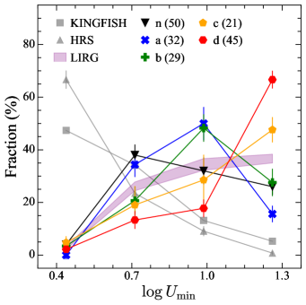
Figure 2: The distributions of $U_{\mathrm{min}}$ in LIRGs are compared with star-forming galaxies from HRS (upward triangles; Boselli et al. 2010; Ciesla et al. 2014) and KINGFISH (squares; Kennicutt et al. 2011; Draine et al. 2007). The the entire LIRG sample is shown in the purple shaded ($\pm 1\sigma$) region. The star-forming and quenched galaxies in the HRS and KINGFISH samples decrease toward high $U_{\mathrm{min}}$, while the LIRGs tend to peak at high values. The peak $U_{\mathrm{min}}$ of the LIRGs increases from non-mergers (“n”, black) to late-stage mergers (“d”, red). The total number of objects at each merger stage with robust SED fits are listed in the legend. The uncertainties are estimated with a Monte Carlo method, resampling the parameters according to their measurement uncertainties and calculating the number of galaxies in each bin 500 times. No error bars are associated with the KINGFISH galaxies because uncertainties are not available for them.

5.3 ISM mass

The dust masses range from $M_{d}=10^{7.0}\,M_{\odot}$ to $10^{8.8}\,M_{\odot}$, with a median value of $10^{8.2\pm 0.3}\,M_{\odot}$. We estimate the gas mass following $\log\,M_{\mathrm{gas}}=\log\,M_{d}+\log\,\delta_{\mathrm{GDR}}+0.23$, where the gas-to-dust ratio $\delta_{\mathrm{GDR}}$ is estimated from the galaxy stellar mass (Shangguan et al. 2018). The corresponding gas masses therefore span $M_{\mathrm{gas}}\approx 10^{9.3}-10^{10.9}\,M_{\odot}$, with a median value of $10^{10.3\pm 0.3}\,M_{\odot}$. F03164$+$4119, a radio-loud AGN, is the only object with $\log\,(M_{\mathrm{gas}}/M_{*})<-1.5$ or $\log\,(M_{d}/M_{*})<-3.5$, significantly lower than the rest of the sample.

It is not trivial to verify the reliability of our dust-based gas masses, as direct H I measurements are lacking for most of our sample. Nevertheless, we tried to compare our results with molecular gas masses for the subsample of 46 GOALS objects with CO measurements compiled by Larson et al. (2016), with the major caveat that the molecular-to-total gas fraction is unknown. Our total gas masses are consistent with the molecular gas masses, with a median difference of $0.09\pm 0.24$ dex. Taken at face value, this might indicate that the molecular gas is able to account for most of the gas in the region of dust emission. However, we have to emphasize that the CO-to-$\mathrm{H_{2}}$ conversion factor adopted in Larson et al. (2016) is $X_{\mathrm{CO}}=3.0\times 10^{20}\,\mathrm{H_{2}\,cm^{-2}\,(K\,km\,s^{-1})^{-1}}$ or $\sim 6.5$ $M_{\odot}\,\mathrm{(K\,km\,s^{-1}\,pc^{2})^{-1}}$, which is $\sim 1.5$ times of the fiducial Milky Way value of $\sim 4.3$ $M_{\odot}\,\mathrm{(K\,km\,s^{-1}\,pc^{2})^{-1}}$ (e.g., Bolatto et al. 2013) and $\sim 8$ times the value found in ULIRGs, $\sim 0.8$ $M_{\odot}\,\mathrm{(K\,km\,s^{-1}\,pc^{2})^{-1}}$. Therefore, this test still suffers considerable uncertainty due to the CO-to-$\mathrm{H_{2}}$ conversion factor.

Figure 3a compares the gas mass fraction of LIRGs with normal galaxies from xCOLD GASS. LIRGs at different merger stages largely occupy a similar region in parameter space, with later merger stages preferentially exhibiting somewhat higher gas mass fractions. By contrast, LIRGs as a group tend to have higher gas fractions than the overall xCOLD GASS sample. This is not unexpected, for LIRGs are mostly starburst systems. Typical main-sequence galaxies (Section 6.1) offer a more appropriate comparison. In Figure 3b, we calculate the $50^{+25}_{-25}$th percentiles of the gas fraction of main-sequence galaxies, taking into account upper limits using the Kaplan-Meier product-limit estimator KMESTM from ASURV (Feigelson & Nelson 1985; Lavalley et al. 1992). LIRGs have moderately higher ($\sim 0.3$ dex) higher gas fractions than the median gas fraction of main-sequence galaxies in the xCOLD GASS sample.

Divided into different phases along the merger sequence (Figure 4), the gas mass fraction of LIRGs tends to rise from the pre-merger stage (“a”) to the late-merger stage (“d”). According to the Kolmogorov-Smirnov statistic, the “d” sample differs statistically significantly from samples “a” and “c” ($p<0.05$), but, formally, not from sample “b” ($p<0.1$). As discussed in Appendix D, the increase of gas fraction toward late-stage mergers holds also for dust masses derived from the modified blackbody (MBB) analysis.

What is the physical origin of the gas enhancement? Since our gas masses are inferred indirectly from dust emission, perhaps the apparent rise in gas mass fraction is an artifact of enhanced dust production in the nuclear starbursts of late-stage mergers (Haan et al. 2013). However, whether starbursts lead to the preferential production or destruction of dust grains is unclear (Gall et al. 2011a, 2011b). The effect, in any case, is only mild, as the gas fractions of LIRGs are only moderately higher than those of main-sequence galaxies. Galaxy-galaxy mergers may increase the supply of cold gas through cooling of hot halo gas (Moster et al. 2011; Hwang & Park 2015; Karman et al. 2015), but the observational evidence of enhanced gas mass fractions in galaxy pairs and post-merger galaxies is not clear-cut (Ellison et al. 2015, 2018; Violino et al. 2018)

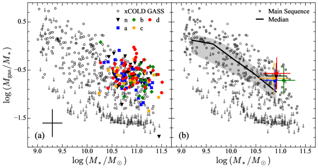
Figure 3: The gas mass fraction of LIRGs in different merger stages are compared with the xCOLD GASS galaxy sample. Individual objects are plotted in (a), while the $50^{+25}_{-25}$th percentile of the gas fractions at different merger stages are plotted in (b). LIRGs in different merger stages are denoted following Figure 2. The galaxies with measured total gas are denoted with empty circles, and those with upper limits are denoted with downward arrows. Galaxies on the main sequence are denoted with filled gray circles in (b). The main sequence galaxies (Figure 5) are selected within $\pm 0.4$ dex of the relation provided by Saintonge et al. (2016; their Equation 5). The median (thick line) and 25th-to-75th percentile (gray shaded region) of gas fraction of the main-sequence galaxies in (b) are calculated with KMESTM including the upper limits. LIRGs tend to have moderately higher gas fraction than main-sequence galaxies.

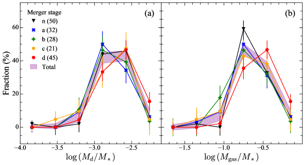
Figure 4: The distribution of (a) dust and (b) gas mass fractions at different merger stages. There is a trend for the gas fraction to increase toward late-merger stages. The gas fraction of the late-stage mergers tends to be significantly different from the other subgroups. The symbols and uncertainties are the same as in Figure 2.

We end this section with a caveat. Recall that our gas mass estimates depend critically on $\delta_{\mathrm{GDR}}$, which ultimately is tied to the mass–metallicity relation of isolated, star-forming galaxies (Tremonti et al. 2004; Kewley et al. 2008). However, galaxy mergers in general (e.g., Ellison et al. 2008; Scudder et al. 2012) and LIRGs in particular (e.g., Rupke et al. 2008; Kilerci Eser et al. 2014) lie systematically below the mass-metallicity relation, by $\sim 0.2$ dex (Herrera-Camus et al. 2018). The metallicity of gravitationally disturbed systems are likely diluted by the inflow of more pristine, low-metallicity gas (Torrey et al. 2012; Bustamante et al. 2018). Taken at face value, a reduction of 0.2 dex in metallicity in LIRGs will lead to an increase of $\delta_{\mathrm{GDR}}$ by the same factor because the two quantities are correlated almost linearly (Leroy et al. 2011; Magdis et al. 2012). On the other hand, the formalism of Shangguan et al. (2018) to convert dust mass into total gas mass explicitly corrects $\delta_{\mathrm{GDR}}$ by a factor of 0.23 dex to account for H I gas from the outskirts of the galaxy. This factor, in fact, is almost exactly identical to the metallicity offset for LIRGs reported by Herrera-Camus et al. (2018), strongly corroborating the scenario that dynamical interactions drive metal-poor H I gas from the outskirts to the center of the galaxy. Our methodology, in other words, is fully applicable to LIRGs despite possible variations in the mass–metallicity relation in these systems. Note, further, the flatness of the mass–metallicity relation at the massive end implies that increasing the stellar mass by a factor of 2 only increases the metallicity by $<0.1$ dex, much smaller than other uncertainties.

6 Discussion

6.1 Star formation rate and the effect of AGNs

The cold dust emission we measure from fitting the photometric SED with the DL07 model presumably emanates from the large-scale ISM of the galaxy. We denote as $L_{\mathrm{galaxy}}$ the $8-1000\,\micron$ integrated luminosity of this component. Although extinction is formally taken into consideration in our fits, it has an almost negligible effect on the DL07 component. The LIRGs with robust fits have $L_{\mathrm{galaxy}}$ $\approx 10^{44.2}$ to $10^{46.0}$ $\mathrm{erg\,s^{-1}}$, with a median value of $10^{45.0\pm 0.3}$ $\mathrm{erg\,s^{-1}}$. Following Kennicutt (1998b; Equation 4), these values of $L_{\mathrm{galaxy}}$ translate to SFRs = 5.9$-$296 $M_{\odot}\>\mathrm{yr^{-1}}$ (median 27 $M_{\odot}\>\mathrm{yr^{-1}}$); in accordance with other conventions throughout this paper, the SFRs refer to a Chabrier (2003) IMF.

As shown in Figure 5a, our sample of LIRGs are located systematically above the galaxy main-sequence, which, for consistency, is represented by the parametric relation of Saintonge et al. (2016) and by galaxies whose SFRs lie within $\pm 0.4$ dex (Chang et al. 2015) of the relation. We note that Saintonge et al. (2016) define the main sequence based on SFRs derived from UV and mid-IR (12 or 22 µm) luminosities of Sloan Digital Sky Survey DR7 galaxies with $0.01<z<0.05$ and $M_{*}>10^{8}\,M_{\odot}$. It is still debatable whether the main sequence flattens beyond $M_{*}\approx 10^{10.5}\,M_{\odot}$. The detailed form of the galaxy main sequence depends on the selection criteria for star-forming galaxies (Renzini & Peng 2015), as well as on the methodology used to derive SFRs (e.g., H$\alpha$ luminosity: Peng et al. 2010; Renzini & Peng 2015; UV+IR luminosity: Whitaker et al. 2012; Lee et al. 2015; Saintonge et al. 2016).

Except for those with the highest SFRs ($\gtrsim 100\,M_{\odot}\,\rm{yr^{-1}}$) and highest stellar masses ($M_{*}\gtrsim 10^{11}\,M_{\odot}$), which are almost exclusively late-stage mergers, LIRGs of different merger stages largely overlap with each other. Considerable uncertainty surrounds the SFRs in LIRGs, however. AGN contamination of FIR-based SFRs remains a possibility (Shangguan et al. 2018). Moreover, AGNs may be hidden by strong dust obscuration, especially in late-stage mergers (e.g., Arp 220; Scoville et al. 2017). Objects with identifiable AGN signatures do not stand out clearly from those that do not in Figure 5b, except that, as with the merger stage, nearly all sources with SFRs $\gtrsim 100\,M_{\odot}\,\rm{yr^{-1}}$ and $M_{*}\gtrsim 10^{11}\,M_{\odot}$ are identified as AGNs.

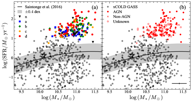
Figure 5: LIRGs lie above the galaxy main sequence (solid line: Saintonge et al. 2016). LIRGs in different merger stages are denoted following Figure 2, and galaxies from the xCOLD GASS sample are plotted as empty circles. The shaded region is $\pm 0.4$ dex above and below the solid line, indicating the range of the main sequence. In (b), LIRGs are divided into AGNs, non-AGNs, and unknown based on all the available diagnostics in the literature (Table 1). The median error bars are shown in the lower-right corner.

6.2 Star formation efficiency

The gas content of star-forming galaxies correlates strongly with their SFR (the Kennicutt-Schmidt relation; Kennicutt 1998a, and references therein). It has been suggested that normal and starburst galaxies follow two different sequences of the Kennicutt-Schmidt relation, both for gas traced through lines (Daddi et al. 2010; Genzel et al. 2010) and indirectly through dust emission (Rowlands et al. 2014). Rowlands et al.’s study combines local ($z<0.5$) dusty galaxies from the Herschel-Astrophysical TeraHertz Large Area Survey (H-ATLAS) and $z\approx 2$ submillimeter galaxies. An important consequence of this result is that for a given amount of gas, starbursts generate stars with greater star formation efficiency, $\mathrm{SFE}\equiv\mathrm{SFR}/M_{\mathrm{gas}}$. Not all investigators accept the reality of this apparent bimodality in SFE, as the result depends on the uncertainty of the CO-to-$\mathrm{H_{2}}$ conversion factor (e.g., Narayanan et al. 2012), the exact formulation of the star formation law (Krumholz et al. 2012), and possible selection effects impacting the CO observations (Sargent et al. 2014).

Our new analysis of the GOALS sample provides a fresh opportunity to re-examine this issue, using our homogeneously derived, robust estimates of the SFRs and ISM masses. Figure 6a shows that the GOALS LIRGs lie essentially in between the two sequences of normal and starburst galaxies defined by Rowlands et al. (2014), in excellent agreement with the behavior of starbursts, as suggested recently (e.g., Saintonge et al. 2011; Sargent et al. 2014; Violino et al. 2018). Different merger stages cannot be clearly distinguished, except for the handful of the most extreme advanced mergers with the highest SFRs ($\gtrsim 100\,M_{\odot}\mathrm{yr^{-1}}$), which also possess the highest SFEs. We zoom in get a better view in Figure 6b, now further highlighting the AGNs. Again, apart from the subset of the most dust-rich systems with the most extreme levels of star formation activity, AGNs do not stand out notably. It is worth noting that the correlation between dust mass and SFR does not arise trivially from their mutual dependence on the IR emission. This issue has been tested by Santini et al. (2014) using mock SEDs of galaxies that cover the parameter space of dust mass and SFR of our LIRGs. This is mainly because the far-IR emission is much more sensitive to the dust temperature than to the dust mass.

Lastly, Figure 7 illustrates the dependence of the gas depletion timescale, $\tau_{\rm dep}\equiv{\rm SFE}^{-1}$, with the specific SFR, ${\rm sSFR}={\rm SFR}/M_{*}$. LIRGs usually have $\tau_{\rm dep}<3$ Gyr, systematically shorter than most normal galaxies. LIRGs and main-sequence galaxies of similar stellar mass ($>10^{10.5}\,M_{\odot}$; black points) clearly follow a trend that is close to the relation between molecular gas depletion timescale and sSFR derived by Saintonge et al. (2011): $\tau_{\mathrm{dep}}(\mathrm{H_{2}})\propto\mathrm{sSFR}^{-0.724}$. LIRGs in different merger stages largely overlap with each other along the trend, indicating that the SFR is not enhanced exclusively during any particular merger stage, although the more advanced stages (“c” and “d”) do tend to have systematically shorter $\tau_{\mathrm{dep}}$ and higher sSFR. But, there are exceptions. Advanced mergers with long $\tau_{\mathrm{dep}}$ and low sSFR do exist. A few late-stage mergers with low SFE have markedly low dust temperatures (e.g., $T_{d}=23.4\pm 0.5$ K in F02070+3857; $T_{d}=20.8\pm 0.4$ K in F05365+6921). It is conceivable that much of the ISM in these systems, despite being advanced mergers, has not yet settled to the center of the galaxy to fuel a nuclear starburst. Depending on the details of the progenitor galaxies and the particulars of the orbital parameters, galaxy-galaxy interactions can enhance gas density and produce extended, clumpy star formation (Powell et al. 2013; Renaud et al. 2014) prior to the onset of a nuclear starburst, which is only triggered after sufficient inflow of cold gas occurs (e.g., Di Matteo et al. 2007; Hopkins et al. 2013). In the opposite extreme, we also find non-mergers with high SFE (e.g., F23135$+$2517, F06592$-$6313, F14179$+$4927); these are perhaps triggered by minor rather than major mergers.

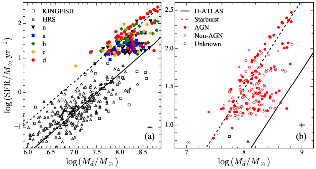
Figure 6: LIRGs tend to have higher SFRs for the same dust mass compared to normal galaxies from the HRS and KINGFISH samples. LIRGs in different merger stages are denoted following Figure 2, while normal galaxies are empty circles. Panel (b) is zoomed in to better show the distribution of the AGNs, non-AGNs, and unknown subsamples of the LIRGs (Table 1). The solid and dashed lines are the relations derived from low-$z$ dusty galaxies (H-ATLAS) and starburst galaxies (local ULIRGs and $z\approx 2$ submillimeter galaxies) by Rowlands et al. (2014), respectively. The median uncertainties are shown on the lower-right corner of each panel.

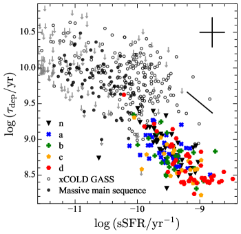
Figure 7: The depletion timescale of the total gas and the specific SFR (sSFR) of LIRGs are compared with galaxies from xCOLD GASS sample. LIRGs in different merger stages are denoted following Figure 2. The empty circles and downward arrows are galaxies from xCOLD GASS with detections and upper limits of the total gas mass, respectively. The filled circles highlight the main-sequence galaxies with stellar mass $>10^{10.5}\,M_{\odot}$. For comparison, the solid black line indicates the slope for the dependence of molecular gas depletion timescale on sSFR from Saintonge et al. (2011): $\tau_{\mathrm{dep}}(\mathrm{H_{2}})\propto\mathrm{sSFR}^{-0.724}$. The median uncertainties are shown on the upper-right corner. LIRGs and massive main-sequence galaxies tend to follow a trend with a slope close to that of the molecular gas depletion timescale.

7 Conclusions

The sample of LIRGs in GOALS encompasses a large, homogeneously selected sample of nearby ($z\lesssim 0.088$), luminous (median $L_{\rm IR}=10^{11.4\pm 0.3}\,L_{\odot}$), massive (median $M_{*}=10^{10.9\pm 0.3}\,M_{\odot}$) star-forming galaxies covering a diverse range of morphologies representing different stages of the galaxy merger sequence. We use a recently developed Bayesian MCMC fitting method to derive global physical parameters (total dust mass, gas mass, extinction, stellar mass, SFR, SFE) for 193 of the 201 GOALS galaxies by modeling their integrated IR ($1-500$ µm) SEDs constructed from 2MASS, WISE, and Herschel photometry. The spectral decomposition of the SEDs also yields useful constraints on the intensity of the ISRF as well as the presence and strength of an AGN torus. Using a subsample of objects with aperture-matched Spitzer/IRS spectra, we demonstrate that robust physical parameters can be measured with the wavelength coverage and quality of the available photometric data. We use these measurements to investigate the ISM content and SFRs of LIRGs, with emphasis on their evolutionary phase along the merger sequence and the effect of AGNs.

The main conclusions are as follows:

1. As expected from their IR selection, LIRGs are rich in dust (and hence gas). The dust masses of LIRGs range from $10^{7.0}$ to $10^{8.8}\,M_{\odot}$, with a median of $10^{8.2\pm 0.3}\,M_{\odot}$; these correspond to total (atomic plus molecular) gas masses of $10^{9.3}$ to $10^{10.9}\,M_{\odot}$ (median $10^{10.3\pm 0.3}\,M_{\odot}$). The gas mass fractions ($M_{\mathrm{gas}}$/$M_{*}$) of LIRGs are $\sim 0.3$ dex higher than those of normal, star-forming galaxies on the main sequence, the most gas-rich being those morphologically classified as late-stage mergers.

2. LIRGs have systematically stronger ISRFs than normal, star-forming galaxies. Moreover, the intensity of the ISRF increases gradually but progressively from early- to late-stage mergers, likely a reflection of elevated ISM concentration and central star formation in advanced stages of the merger sequence.

3. The integrated IR ($8-1000\,\micron$) luminosities traced by the global, cold dust component implies SFRs of 5.9 to 296 $M_{\odot}\>\mathrm{yr^{-1}}$ (median 27 $M_{\odot}\>\mathrm{yr^{-1}}$), placing these LIRGs systematically above the galaxy star-forming main sequence. While different merger stages and levels of AGN activity show no strong correlation with location on the main sequence, objects with $\mathrm{SFR}\gtrsim 100$ $M_{\odot}\>\mathrm{yr^{-1}}$ and $M_{*}\gtrsim 10^{11}\,M_{\odot}$ are all advanced, late-stage mergers with unambiguous signatures of AGNs.

4. LIRGs fill the gap in the bimodal distribution of SFEs previously defined by normal star-forming galaxies and starburst galaxies. Advanced mergers tend to exhibit systematically higher SFEs, while the variation of SFE is large among all the merger stages. LIRGs obey and extend toward higher masses the trend between molecular gas depletion timescale and specific SFR defined by main-sequence galaxies.

Appendix A Spitzer/IRS spectra

The mid-IR IRS spectra provide crucial information to constrain the torus and cold dust emission. Although IRS spectra exist for the entire GOALS sample, a major difficulty is that most of our targets are relatively nearby galaxies that have spatial extents larger than the IRS slit widths (3$\farcs$7 for SL and 10$\farcs$6 for LL). We visually checked the slit coverage of each object using available optical and near-IR images and conclude that 61 of the GOALS galaxies do not suffer from this aperture mismatch problem. We obtain their IRS low-resolution spectra from the NASA/IPAC Infrared Science Archive. The spectra were extracted with the standard extraction aperture and point source calibration modes in SPICE (Stierwalt et al. 2013). The different orders of the SL and LL spectra are matched. Since the slit width of SL is much smaller than that of LL, the flux level of the SL spectra is usually lower than that of the LL spectra, and the former needs to be scaled up to match the latter based on their overlapping region (Stierwalt et al. 2013). However, this method does not always provide an optimal scaling factor because the overlapping region may be affected by emission/absorption features and sometimes by the poor signal-to-noise ratio of the edge of the spectra. Therefore, we fine tune the scaling factor of SL by eye to achieve $\sim 5$% accuracy. We further scale the internally adjusted IRS spectra to match the integrated flux density of the WISE  $W$4 band. The scaling factors of both steps are listed in Table 3; they are usually less than 30%. Rigorously speaking, the aperture mismatches among SL, LL, and the integrated photometry may introduce systematic uncertainties into the SED fitting. However, this problem is beyond the scope of this work. Appendix B tests the consistency between the SED fits with and without IRS spectra and demonstrates that the currently available data are sufficiently accurate for our main goals.

Appendix B SED Fits with IRS Spectra

In order to test the robustness of the physical quantities derived from fitting the photometric SED alone, we select a subsample of 61 objects whose IRS spectra are least affected by aperture mismatch (Appendix A). The IRS spectra provide abundant mid-IR features that allow SED fits with more detailed models. Unlike the fits with photometric data only, we adopt CAT3D torus models with a wind component (Hönig & Kishimoto 2017). The same extinction is applied to the torus and DL07 components. In principle, the torus and DL07 components may suffer different levels of extinction because the torus resides in the nucleus while the galactic dust is distributed more extensively. However, allowing for separate extinctions for the torus and DL07 components do not significantly improve the fits. All 9 parameters of the torus model, as well as $q_{\mathrm{PAH}}$ and $\gamma$ for the DL07 component, are set free, in addition to the other free parameters used for the photometric SED fitting (Table 2). The results are shown in Figure 8. In contrast to Figure 1, data with IRS spectra better constrain the SED models, especially the torus and the silicate absorptions governed by the mid-IR extinction (see panel (b)–(d) of Figure 1 and Figure 8). F08572$+$3915 was not well fit with the photometric data alone; from its IRS spectrum, we know that this object is highly absorbed in the mid-IR, a characteristic not revealed by the photometry alone. Nevertheless, even with the addition of the IRS spectrum the best-fit model still lies systematically below the data at 70–160 µm, although $U_{\mathrm{min}}$ has reached the maximum. The poor fit with the photometric SED likely is also due, at least in part, to this problem.

We further confirm that, apart from the seven objects with distinctly bad fits to the photometric SED, the best-fit results with and without the IRS spectra are consistent. The two sets of fits give very well-matched best-fit parameters for the DL07 component (Figure 9). Objects that show less robust photometric SED fits tend to have lower $U_{\mathrm{min}}$ and $L_{\mathrm{galaxy}}$ (Figure 10a), likely because of overestimation of the torus component. Fortunately, the dust mass is always very well matched. For the case of F08572$+$3915 (Figure 1d and Figure 8), this is likely because $U_{\mathrm{min}}$ and $L_{\mathrm{galaxy}}$ decrease together. When the torus occupies more of the emission from the cold dust component, it pushes the DL07 component to peak at even longer wavelengths (lower $U_{\mathrm{min}}$), such that given the same amount of emission more dust mass is required. This effect balances the dust mass. As shown in Figure 10b, the torus luminosity and the fractional contribution of the torus emission to the total far-IR (8–1000 µm) are also reasonably constrained from the photometric SED fitting, albeit with $\sim 50\%$ systematic overestimation. It is partly because $\tau_{9.7}$ is usually underestimated from the photometric SED fit unless $\tau_{9.7}$ is significant (e.g., $\gtrsim 2$). Nevertheless, all of the objects showing significant inconsistency between the photometric and full SED fits turns out to be successfully identified by visual inspection of the photometric fits.

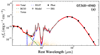
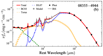
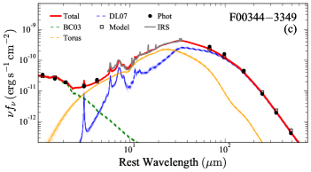
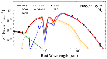
Figure 8: Examples of SED fits using IRS spectra. The symbols are the same as in Figure 1. The gray histogram plots the IRS spectrum.

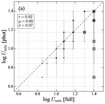
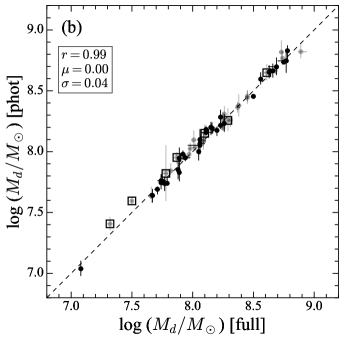
Figure 9: Comparison of the best-fit (a) $U_{\mathrm{min}}$ and (b) $M_{d}$ of the cold dust emission derived from SED fits using only photometric data versus those that incorporate full spectroscopic data from Spitzer/IRS. The consistency is good. Since $U_{\mathrm{min}}$ is a discrete parameter, the results are located on the dashed grids and sometimes overlap with each other; the errors are not resolvable if they are smaller than the grid size. In panel (a), points with darker shade correspond to more objects. In panel (b), the black circles are objects with $\mathrm{log}\,\tau_{9.7}<0.3$, while the gray symbols are the rest of the objects with high mid-IR extinction. Objects highlighted with boxes are those with photometric SEDs that are visually identified as having less robust fits (e.g., F08572$+$3915 in Figure 1d). The legend in the upper-left corner shows the Pearson’s correlation coefficient ($r$) of the two quantities, and the median ($\mu$) standard deviation ($\sigma$) of their differences ($y-x$). The uncertain objects marked with boxes are excluded from the statistics. The dashed line shows the 1:1 relation.

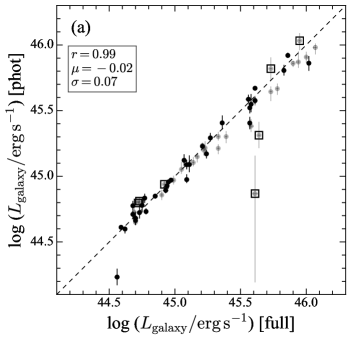
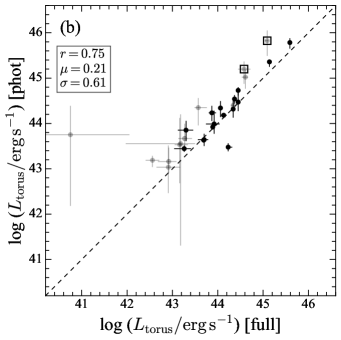
Figure 10: The best-fit IR ($8-1000$ µm) luminosity of (a) the galaxy ($L_{\mathrm{galaxy}}$) and (b) dust torus ($L_{\mathrm{torus}}$) using photometric and full SEDs are reasonably consistent with each other for the robustly fitted objects. The symbols are the same as in Figure 9.

Appendix C Comparison between the stellar mass and star formation rate

The stellar masses and SFRs for a large fraction of the GOALS galaxies were also derived by Howell et al. (2010; their Table 3). They estimated the integrated stellar mass using 2MASS $K_{s}$-band luminosity, supplemented with Spitzer/IRAC 3.6 µm photometry. They assumed a $M/L$ according to Lacey et al. (2008), who assumed an IMF close to that of Kroupa (2001) for quiescent galaxies and a top-heavy IMF for starburst galaxies. Since it is not straightforward to convert their IMFs to our choice of Chabrier (2003) IMF, we directly compare our newly derived $M_{*}$ with Howell et al.’s results (Figure 11a). Howell et al. did not consider AGN torus emission, which may significantly contaminate the $K_{s}$ and IRAC 3.6 µm bands. We use the fraction of torus emission derived from our analysis to evaluate the possible bias of $M_{*}$. Objects with high torus fractions tend to exhibit the largest systematic deviations between the two sets of measurements. Excluding the objects with the most significant torus emission ($\log\,L_{\mathrm{torus}}/L_{\mathrm{total}}>-0.6$), our stellar masses are still systematically lower than those of Howell et al. by $0.15\pm 0.13$ dex. This is likely due to the different choices of $M/L$, including the effect of different IMFs. Nevertheless, considering the typical 0.2 dex uncertainty of stellar masses (Conroy 2013), this level of discrepancy is not serious. In fact, our stellar masses are on average $0.15\pm 0.31$ dex higher than those of U et al. (2012), in spite of the same (Chabrier) IMF used in both. Further detailed study of the full UV-to-IR SED is necessary to derive more robust stellar masses, but this is outside of the scope of the current work.

Howell et al. (2010) calculated SFRs using the formalism of Kennicutt (1998b) that combines UV and IR emission. We divide their SFRs by a factor of 1.5 to convert their scale based on the Salpeter IMF to that of the Chabrier IMF. As Howell et al. caution, some of their SFRs are severely affected by AGN contamination (Figure 11b). Excluding the objects with torus fractions $\gtrsim$ 25%, we find that Howell et al.’s SFRs are consistent with ours.

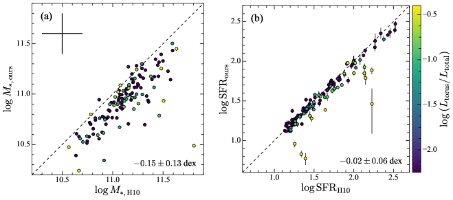
Figure 11: Comparison of our newly measured (a) stellar masses and (b) SFRs with those provided by Howell et al. (2010; H10). The fractional contribution of the torus ($L_{\mathrm{torus}}$) to the total IR luminosity ($L_{\mathrm{torus}}$+$L_{\mathrm{galaxy}}$) is color coded with the right color bar. The torus fraction is zero (dark purple) for objects fitted without a torus component. Some objects with a high torus fraction tend to have $M_{*}$ and SFR overestimated by H10, confirming that it is necessary to decompose the torus emission in order to robustly measure the two quantities. The median and standard deviation of the difference ($y-x$) for objects with torus fraction $\lesssim 25\%$ are shown in the lower-right corner. The median uncertainty of our $M_{\mathrm{*}}$ measurements and a typical error bar of 0.2 dex from H10 are shown at the upper-left corner of (a). The systematic deviation of $M_{\mathrm{*}}$ is not significant given the typical uncertainty; it is likely due to the choice of mass-to-light ratio. The two sets of SFRs are in good agreement.

Appendix D Dust masses from the modified blackbody model

The templates provided by DL07 are limited to $U_{\mathrm{min}}\leq 25$. Some of the LIRGs in our sample saturate at this limit, and their fits can still be improved. The dust masses may be overestimated in these objects. This is a non-trivial point, in light of our conclusion that late-stage mergers have higher gas mass fractions than the earlier stages (Figure 4). As $U_{\mathrm{min}}$ tends to increase toward later stage mergers (Figure 2), their apparently higher gas mass fractions may be an artifact. In order to quantify this possible bias on the dust mass and test the robustness of the gas fraction distribution, we obtain an alternative estimate of the dust mass by fitting the far-IR (100 to 500 µm) SED with the MBB model:

$$f_{\mathrm{\nu,MBB}}=\frac{(1+z)^{2}\,M_{d}\,\kappa_{\mathrm{abs}}(\lambda_{0})\,(\lambda_{0}/\lambda)^{\beta}\,B_{\nu}(T_{d})}{D_{L}^{2}},$$ (D1)

where $f_{\mathrm{\nu,MBB}}$ is the rest-frame flux density, $D_{L}$ is the luminosity distance, $z$ is the redshift, and $B_{\nu}(T_{d})$ is the Planck function with dust temperature $T_{d}$. Following Bianchi (2013), we adopt the grain absorption cross-section per unit mass at 250 µm, $\kappa_{\mathrm{abs}}(250\,\micron)=4.0\,\mathrm{cm^{2}g^{-1}}$, and fix $\beta=2.08$. Our method is adapted from Shangguan et al. (2018), who provide a detailed comparison between the MBB and DL07 models.

As Figure 12a shows, the dust masses derived from the two methods agree with each other extremely well for the entire sample. The median deviation is 0.01 dex, and the standard deviation is 0.04 dex. The deviation indeed increases as a function of $U_{\mathrm{min}}$ or $T_{d}$ (Figure 13), but hardly beyond 0.2 dex. F08572+3915, whose torus emission and mid-IR extinction are both very strong, is the only object whose dust mass deviates by more than 0.2 dex between the two methods. The poor quality of its SED fit can be readily identified. In sharp contrast, the dust masses of U et al. (2012; U12) are systematically and severely understimated, by $\sim 0.9$ dex (Figure 12b). U12 derived dust masses by fitting the mid-IR to far-IR SED with a truncated power-law plus an MBB models (Casey 2012). The main reason that U12 systematically underestimated their dust masses is probably because they adopted a too large value of the grain absorption cross-section per unit mass. U12 quote $\kappa_{\mathrm{abs}}(850\,\micron)=0.15\,\mathrm{m^{2}\,kg^{-1}}$ referring to Weingartner & Draine (2001) and Dunne et al. (2003). Weingartner & Draine (2001) provide a much lower value of $\kappa_{\mathrm{abs}}(850\,\micron)=0.0383\,\mathrm{m^{2}\,kg^{-1}}$ (Draine 2003), while $0.15\,\mathrm{m^{2}\,kg^{-1}}$ is the upper limit for the diffuse ISM of extragalactic systems quoted by Dunne et al. (2003). This could account for $\sim 0.6$ dex of the deviation. Moreover, the dust temperature derived by U12 is also systematically higher than ours (median difference $3.6\pm 4.3$ K), likely due to their simplified modeling. This may also contribute to the systematic deviation in dust mass.

Figure 14 reexamines the results presented in Figure 4 concerning the distributions of dust and gas mass fractions as a function of galaxy merger stage, using dust masses derived from MBB fits instead of DL07 models. The two sets of results are indistinguishable.

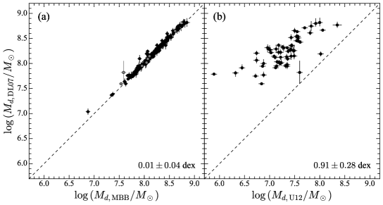
Figure 12: Comparison of our dust masses derived from DL07 models fit to the 100–500 µm SED with (a) dust masses obtained from MBB models fit to the same data and (b) dust masses published by U et al. (2012; U12). The consistency with the MBB-derived dust masses is very good, with median deviation 0.01 dex and standard deviation 0.04 dex. The gray circles are objects less robustly fitted with the DL07 model. By comparison, the dust masses of U12 are significantly lower ($0.91\pm 0.28$ dex) than ours.

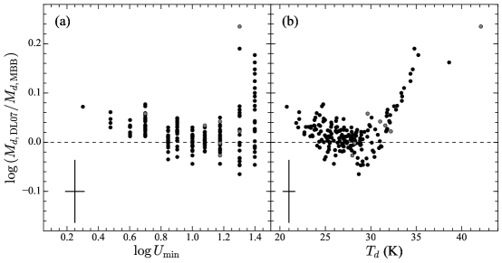
Figure 13: The deviation of the dust mass (between DL07 and MBB) is plotted against (a) $U_{\mathrm{min}}$ and (b) $T_{d}$. For objects with $U_{\mathrm{min}}<25$ or $T_{d}\lesssim 33$ K, the deviation is within $\sim$0.1 dex. However, at $U_{\mathrm{min}}=25$ or $T_{d}>33$ K, the DL07 dust mass is systematically higher than the MBB dust mass, which is exactly as expected because the DL07 templates are limited by $U_{\mathrm{min}}\leq 25$. However, even the highest deviation ($\sim 0.2$ dex) is still moderate.

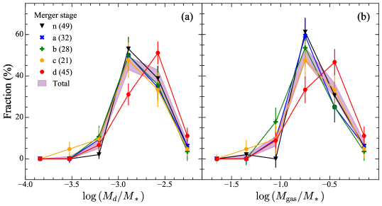
Figure 14: Same as Figure 4, except that the dust (and gas) masses are based on the MBB model. There is not much difference between the distributions based on the two sets of models.

Table 1: Physical Properties of the Sample

Name	$z$	$D_{L}$	Merger	AGN	References	$\mathrm{log}\,M_{*}$	$\mathrm{log}\,\tau_{9.7}$	$\mathrm{log}\,L_{\mathrm{torus}}$	$\mathrm{log}\,L_{\mathrm{galaxy}}$	$\mathrm{log}\,U_{\mathrm{min}}$	$\mathrm{log}\,M_{d}$	$\mathrm{log}\,\delta_{\mathrm{GDR}}$	$\mathrm{log}\,M_{\mathrm{gas}}$	$\mathrm{log}\,\mathrm{SFR}$
		(Mpc)	Stage			($M_{\odot}$)		($\mathrm{erg\,s^{-1}}$)	($\mathrm{erg\,s^{-1}}$)		($M_{\odot}$)		($M_{\odot}$)	($M_{\odot}\,\mathrm{yr^{-1}}$)
(1)	(2)	(3)	(4)	(5)	(6)	(7)	(8)	(9)	(10)	(11)	(12)	(13)	(14)	(15)
F00073$+$2538	0.0152	67.2	b	N	23	$11.12\pm 0.20$	$-0.16^{+0.32}_{-0.41}$	$\cdots$	$44.64^{+0.01}_{-0.01}$	$0.85^{+0.06}_{-0.00}$	$7.96^{+0.02}_{-0.02}$	2.08	$10.04\pm 0.20$	$1.12^{+0.02}_{-0.01}$
F00085$-$1223	0.0196	86.7	d	Y	20, 23	$10.76\pm 0.20$	$-1.10^{+1.39}_{-1.93}$	$\cdots$	$45.05^{+0.04}_{-0.04}$	$1.30^{+0.10}_{-0.12}$	$7.77^{+0.07}_{-0.05}$	2.10	$9.86\pm 0.20$	$1.47^{+0.04}_{-0.04}$
F00163$-$1039	0.0273	121.1	b	N	23	$10.91\pm 0.20$	$-2.37^{+1.32}_{-1.17}$	$44.28^{+0.03}_{-0.04}$	$44.97^{+0.03}_{-0.02}$	$1.00^{+0.08}_{-0.00}$	$8.12^{+0.03}_{-0.04}$	2.09	$10.25\pm 0.21$	$1.56^{+0.02}_{-0.02}$
F00344$-$3349	0.0206	91.8	c	N	23	$10.24\pm 0.20$	$0.47^{+0.15}_{-0.34}$	$44.73^{+0.07}_{-0.11}$	$44.23^{+0.06}_{-0.06}$	$1.40^{+0.00}_{-0.10}$	$7.04^{+0.07}_{-0.06}$	2.17	$9.26\pm 0.21$	$0.77^{+0.07}_{-0.08}$
F00402$-$2349	0.0226	100.3	b	Y	18, 23	$11.30\pm 0.20$	$-2.96^{+1.22}_{-0.72}$	$43.81^{+0.06}_{-0.04}$	$45.10^{+0.01}_{-0.02}$	$1.00^{+0.00}_{-0.00}$	$8.27^{+0.02}_{-0.01}$	2.09	$10.35\pm 0.20$	$1.58^{+0.02}_{-0.01}$
F00506$+$7248	0.0157	72.0	c	N	2	$10.61\pm 0.20$	$-2.24^{+1.30}_{-1.26}$	$44.05^{+0.13}_{-0.27}$	$45.06^{+0.06}_{-0.07}$	$1.18^{+0.22}_{-0.10}$	$7.98^{+0.08}_{-0.08}$	2.11	$10.16\pm 0.21$	$1.57^{+0.05}_{-0.03}$
F00548$+$4331	0.0181	80.2	a	$\cdots$	$\cdots$	$11.04\pm 0.20$	$-1.51^{+1.42}_{-1.77}$	$\cdots$	$44.77^{+0.03}_{-0.02}$	$1.00^{+0.08}_{-0.00}$	$7.89^{+0.04}_{-0.04}$	2.08	$9.95\pm 0.24$	$1.22^{+0.07}_{-0.05}$
F01053$-$1746	0.0201	88.2	c	N	23	$10.85\pm 0.20$	$-0.57^{+0.28}_{-0.51}$	$44.39^{+0.03}_{-0.03}$	$45.19^{+0.02}_{-0.02}$	$1.08^{+0.00}_{-0.00}$	$8.27^{+0.02}_{-0.02}$	2.09	$10.37\pm 0.20$	$1.67^{+0.02}_{-0.02}$
F01076$-$1707	0.0351	156.5	n	N	23	$11.15\pm 0.20$	$-1.35^{+1.37}_{-1.76}$	$\cdots$	$45.29^{+0.04}_{-0.03}$	$1.18^{+0.12}_{-0.10}$	$8.28^{+0.06}_{-0.07}$	2.08	$10.37\pm 0.21$	$1.76^{+0.03}_{-0.02}$
F01159$-$4443	0.0229	102.7	b	N	23	$11.05\pm 0.20$	$-0.94^{+0.98}_{-1.89}$	$\cdots$	$45.03^{+0.02}_{-0.02}$	$1.08^{+0.10}_{-0.08}$	$7.93^{+0.05}_{-0.05}$	2.08	$10.01\pm 0.21$	$1.51^{+0.02}_{-0.02}$
F01173$+$1405	0.0312	137.9	b	N	23	$10.59\pm 0.20$	$-0.37^{+0.54}_{-1.07}$	$44.23^{+0.15}_{-0.18}$	$45.17^{+0.03}_{-0.04}$	$1.40^{+0.00}_{-0.00}$	$7.95^{+0.03}_{-0.03}$	2.12	$10.07\pm 0.20$	$1.65^{+0.02}_{-0.03}$
F01325$-$3623	0.0159	70.6	n	$\cdots$	$\cdots$	$10.75\pm 0.20$	$-1.48^{+1.47}_{-1.72}$	$\cdots$	$44.66^{+0.04}_{-0.03}$	$0.85^{+0.06}_{-0.15}$	$8.10^{+0.09}_{-0.06}$	2.10	$10.19\pm 0.21$	$1.14^{+0.03}_{-0.04}$
F01341$-$3735	0.0173	76.9	a	N	23	$10.87\pm 0.20$	$-0.93^{+1.04}_{-1.95}$	$\cdots$	$44.74^{+0.02}_{-0.02}$	$0.90^{+0.10}_{-0.06}$	$7.94^{+0.04}_{-0.05}$	2.09	$10.04\pm 0.20$	$1.23^{+0.02}_{-0.02}$
F01364$-$1042	0.0483	216.9	d	N	23	$10.39\pm 0.22$	$1.26^{+0.04}_{-0.05}$	$\cdots$	$45.51^{+0.03}_{-0.04}$	$1.30^{+0.00}_{-0.22}$	$8.09^{+0.05}_{-0.04}$	2.15	$10.23\pm 0.20$	$1.97^{+0.03}_{-0.03}$
F01417$+$1651	0.0274	120.3	a	Y	23	$10.42\pm 0.20$	$0.35^{+0.60}_{-2.29}$	$\cdots$	$45.12^{+0.07}_{-0.05}$	$1.30^{+0.10}_{-0.12}$	$7.95^{+0.07}_{-0.06}$	2.14	$10.09\pm 0.21$	$1.59^{+0.06}_{-0.05}$

Note. — (1) Source name. (2) Redshift from NASA/IPAC Extragalactic Database (NED). (3) The luminosity distance in Mpc derived by correcting the heliocentric velocity for the 3-attractor flow model of Mould et al. (2000) using $\Omega_{m}=0.308$, $\Omega_{\Lambda}=0.692$, and $H_{0}=67.8\,\mathrm{km\,s^{-1}\,Mpc^{-1}}$ (Planck Collaboration et al. 2016). (4) The merger stage adopted from Stierwalt et al (2013): n = nonmerger, a = pre-merger, b = early-stage merger, c = mid-stage merger, and d = late-stage merger. Ten objects marked as “?” are not included in Stierwalt et al. (2013). (5) Type of nuclear activity. (6) References for nuclear activity. (7) Stellar mass derived from optical color and $J$-band absolute magnitude (Bell & de Jong 2001), converted to Chabrier (2003) IMF. (8) The optical depth at 9.7 µm. (9) The IR (8–1000 µm) luminosity of the torus derived from the SED fitting. (10) The IR (8–1000 µm) luminosity of the host galaxy cold dust emission derived from the SED fitting. The best-fit extinction model is applied when calculating both $L_{\mathrm{torus}}$ and $L_{\mathrm{galaxy}}$. (11) Best-fit minimum intensity of the interstellar radiation field relative to that measured in the solar neighborhood. The quoted uncertainties represent the 68% confidence interval determined from the 16th and 84th percentile of the marginalized posterior probability density function. However, for some objects, the probability density function is not well resolved, and the lower (or upper) uncertainty is reported as “0.00”. (12) Best-fit total dust mass. (13) Gas-to-dust ratio estimated in Section 5.3. (14) Total gas mass including helium and heavier elements. (15) The SFR calculated from $L_{\mathrm{galaxy}}$ (Col. 10) using the Equation (4) of Kennicutt (1998b) converted to the Chabrier (2003) IMF by dividing by a factor of 1.5.

References: (1) Albrecht et al. (2007); (2) Alonso-Herrero et al. (2009); (3) Alonso-Herrero et al. (2012); (4) Baan et al. (1998); (5) Corbett et al. (2003); (6) Farrah et al. (2007); (7) Gonçalves et al. (1999); (8) Ho et al. (1997); (9) Imanishi (2006); (10) Iwasawa et al. (2011); (11) Inami et al. (2013); (12) Kinney et al. (1993); (13) Koss et al. (2013); (14) Lípari et al. (2000); (15) Masetti et al. (2008); (16) Nardini et al. (2010); (17) Ohyama et al. (2015); (18) Petric et al. (2011); (19) Ricci et al. (2016); (20) Ricci et al. (2017); (21) Tueller et al. (2008); (22) Torres-Albà et al.(2018); (23) Yuan et al. (2010); (24) Zink et al. (2000).

(This table is available in its entirety in machine-readable form.)

Table 2: Model Parameters and Priors

Models	Parameters	Units	Discreteness	Priors
(1)	(2)	(3)	(4)	(5)
BC03	$M_{*}$	$M_{\odot}$	✘	[$10^{6}$, $10^{14}$]
	$t$	Gyr	✔	5 (fixed)
Extinction	$\tau_{9.7}$	–	✔	[$10^{-4}$, $10^{1.5}$]
	$i$	–	✔	[0.0, 90.0]
	$a$	–	✔	[-2.5, -0.25] or [-3.0, -0.5]
CAT3D	$N_{0}$	–	✔	[5.0, 10.0]
(Basic)	$h$	–	✔	[0.25, 1.5] or [0.1, 0.5]
	$L$	$\mathrm{erg\>s^{-1}}$	✘	[$10^{38}$, $10^{48}$]
(Wind)	$f_{\mathrm{wd}}$	–	✔	[0.15, 1.75]
	$a_{w}$	–	✔	[-2.5, -0.5]
	$\theta_{w}$	–	✔	[30, 45]
	$\sigma_{\theta}$	–	✔	[7.5, 15]
DL07	$U_{\mathrm{min}}$	–	✔	[0.10, 25.0]
	$U_{\mathrm{max}}$	–	✔	$10^{6}$ (fixed)
	$\alpha$	–	✘	2 (fixed)
	$q_{\mathrm{PAH}}$	–	✔	0.47 (fixed) or [0.3, 5.0]
	$\gamma$	–	✘	0.03 (fixed) or [0.0, 1.0]
	$M_{d}$	$M_{\odot}$	✘	[$10^{5}$, $10^{11}$]

Table 3: Objects with Spitzer/IRS spectra

Name	$f_{\mathrm{SL}}$	$f_{\mathrm{IRS}}$	$\mathrm{log}\,\tau_{9.7}$	$\mathrm{log}\,U_{\mathrm{min}}$	$\mathrm{log}\,M_{d}$	$\mathrm{log}\,L_{\mathrm{torus}}$	$\mathrm{log}\,L_{\mathrm{galaxy}}$
					($M_{\odot}$)	($\mathrm{erg\,s^{-1}}$)	($\mathrm{erg\,s^{-1}}$)
(1)	(2)	(3)	(4)	(5)	(6)	(7)	(8)
F00344$-$3349	1.15	1.14	$-0.14^{+0.05}_{-0.06}$	1.40	$7.08^{+0.02}_{-0.02}$	$44.45^{+0.02}_{-0.01}$	$44.56^{+0.01}_{-0.02}$
F01076$-$1707	1.15	1.12	$-0.04^{+0.09}_{-0.09}$	1.30	$8.23^{+0.02}_{-0.02}$	$44.15^{+0.10}_{-0.14}$	$45.27^{+0.01}_{-0.01}$
F01173$+$1405	1.18	1.10	$0.26^{+0.03}_{-0.03}$	1.40	$7.94^{+0.04}_{-0.02}$	$43.87^{+0.09}_{-0.07}$	$45.24^{+0.01}_{-0.01}$
F01325$-$3623	1.40	1.11	$0.25^{+0.03}_{-0.04}$	0.90	$8.06^{+0.02}_{-0.02}$	$41.24^{+0.87}_{-1.04}$	$44.70^{+0.01}_{-0.01}$
F02208$+$4744	1.14	1.16	$0.06^{+0.04}_{-0.05}$	1.08	$7.88^{+0.02}_{-0.02}$	$42.34^{+0.18}_{-0.27}$	$44.73^{+0.01}_{-0.01}$
F02437$+$2122	1.10	1.00	$0.31^{+0.04}_{-0.03}$	1.18	$7.66^{+0.02}_{-0.02}$	$43.09^{+0.06}_{-0.10}$	$44.69^{+0.01}_{-0.01}$
F03117$+$4151	1.23	1.14	$0.04^{+0.14}_{-0.21}$	1.00	$8.11^{+0.06}_{-0.04}$	$44.13^{+0.07}_{-0.07}$	$44.93^{+0.02}_{-0.02}$
F04118$-$3207	1.26	1.11	$-0.08^{+0.10}_{-0.13}$	1.08	$7.71^{+0.02}_{-0.02}$	$43.69^{+0.04}_{-0.06}$	$44.59^{+0.01}_{-0.01}$
04271$+$3849	1.25	1.09	$0.13^{+0.06}_{-0.06}$	1.00	$7.89^{+0.03}_{-0.02}$	$42.11^{+0.61}_{-1.52}$	$44.70^{+0.02}_{-0.01}$
F04454$-$4838	1.00	1.14	$0.99^{+0.05}_{-0.05}$	1.40	$8.01^{+0.02}_{-0.02}$	$43.57^{+0.20}_{-0.21}$	$45.39^{+0.01}_{-0.01}$

Note. — (1) Model components. (2) The parameters of each model. (3) The units of the parameters. (4) Whether the parameter is discrete and requires interpolation to implement the MCMC fitting. (5) The range of the priors. For parameters with two priors, the first is for the fits with photometric SEDs, while the second is for the fits with the full SEDs.

Note. — (1) Source name. (2) The scaling factor to match the SL to LL spectra. (3) The scaling factor to match the IRS spectra to $W$4 band. (4) The MIR extinction indicated as the optical depth at 9.7 µm. (5) The $U_{\mathrm{min}}$ of the interstellar radiation field. The uncertainties are not resolved for most of the object, so they are not listed. (6) The dust mass. (7) The integrated luminosity of the dust torus at 8–1000 µm. (8) The integrated luminosity of the host galaxy cold dust emission at 8–1000 µm.

(This table is available in its entirety in machine-readable form.)

References

- Albrecht et al. (2007) Albrecht, M., Krügel, E., & Chini, R. 2007, A&A, 462, 575
- Alonso-Herrero et al. (2009) Alonso-Herrero, A., García-Marín, M., Monreal-Ibero, A., et al. 2009, A&A, 506, 1541
- Alonso-Herrero et al. (2012) Alonso-Herrero, A., Pereira-Santaella, M., Rieke, G. H., & Rigopoulou, D. 2012, ApJ, 744, 2
- Armus et al. (2009) Armus, L., Mazzarella, J. M., Evans, A. S., et al. 2009, PASP, 121, 559
- Arribas et al. (2004) Arribas, S., Bushouse, H., Lucas, R. A., Colina, L., & Borne, K. D. 2004, AJ, 127, 2522
- Astropy Collaboration et al. (2013) Astropy Collaboration, Robitaille, T. P., Tollerud, E. J., et al. 2013, A&A, 558, A33
- Baan et al. (1998) Baan, W. A., Salzer, J. J., & LeWinter, R. D. 1998, ApJ, 509, 633
- Barnes & Hernquist (1996) Barnes, J. E., & Hernquist, L. 1996, ApJ, 471, 115
- Bell & de Jong (2001) Bell, E. F., & de Jong, R. S. 2001, ApJ, 550, 212
- Bell et al. (2003) Bell, E. F., McIntosh, D. H., Katz, N., & Weinberg, M. D. 2003, ApJS, 149, 289
- Bianchi (2013) Bianchi, S. 2013, A&A, 552, A89
- Blanton & Roweis (2007) Blanton, M. R., & Roweis, S. 2007, AJ, 133, 734
- Blecha et al. (2018) Blecha, L., Snyder, G. F., Satyapal, S., et al. 2018, MNRAS, 478, 3056
- Bolatto et al. (2013) Bolatto, A. D., Wolfire, M., & Leroy, A. K. 2013, ARA&A, 51, 207
- Boselli et al. (2010) Boselli, A., Eales, S., Cortese, L., et al. 2010, PASP, 122, 261
- Bournaud et al. (2011) Bournaud, F., Powell, L. C., Chapon, D., & Teyssier, R. 2011, in IAU Symp. 271, Astrophysical Dynamics: From Stars to Galaxies, 160
- Bruzual & Charlot (2003) Bruzual, G., & Charlot, S. 2003, MNRAS, 344, 1000
- Bryant & Scoville (1999) Bryant, P. M., & Scoville, N. Z. 1999, AJ, 117, 2632
- Bustamante et al. (2018) Bustamante, S., Sparre, M., Springel, V., & Grand, R. J. J. 2018, MNRAS, 479, 3381
- Casey (2012) Casey, C. M. 2012, MNRAS, 425, 3094
- Chabrier (2003) Chabrier, G. 2003, PASP, 115, 763
- Chang, et al. (2015) Chang, Y.-Y., van der Wel, A., da Cunha, E., et al. 2015, ApJS, 219, 8
- Chapman et al. (2005) Chapman, S. C., Blain, A. W., Smail, I., & Ivison, R. J. 2005, ApJ, 622, 772
- Chu et al. (2017) Chu, J. K., Sanders, D. B., Larson, K. L., et al. 2017, ApJS, 229, 25
- Ciesla, et al. (2014) Ciesla, L., Boquien, M., Boselli, A., et al. 2014, A&A, 565, A128
- Conroy (2013) Conroy, C. 2013, ARA&A, 51, 393
- Corbett et al. (2003) Corbett, E. A., Kewley, L., Appleton, P. N., et al. 2003, ApJ, 583, 670
- da Cunha et al. (2010) da Cunha, E., Charmandaris, V., Díaz-Santos, T., et al. 2010, A&A, 523, A78
- Daddi, et al. (2007) Daddi, E., Dickinson, M., Morrison, G., et al. 2007, ApJ, 670, 156
- Daddi et al. (2010) Daddi, E., Elbaz, D., Walter, F., et al. 2010, ApJ, 714, L118
- Di Matteo, et al. (2007) Di Matteo, P., Combes, F., Melchior, A.-L., et al. 2007, A&A, 468, 61
- Di Matteo et al. (2005) Di Matteo, T., Springel, V., & Hernquist, L. 2005, Nature, 433, 604
- Dinh-V-Trung et al. (2001) Dinh-V-Trung,, Lo, K. Y., Kim, D.-C., Gao, Y., & Gruendl, R. A. 2001, ApJ, 556, 141
- Downes & Solomon (1998) Downes, D., & Solomon, P. M. 1998, ApJ, 507, 615
- Draine (2003) Draine, B. T. 2003, ARA&A, 41, 241
- Draine et al. (2007) Draine, B. T., Dale, D. A., Bendo, G., et al. 2007, ApJ, 663, 866
- Draine & Li (2007) Draine, B. T., & Li, A. 2007, ApJ, 657, 810
- Dunne et al. (2003) Dunne, L., Eales, S., Ivison, R., et al. 2003, Nature, 424, 285
- Elbaz et al. (2002) Elbaz, D., Cesarsky, C. J., Chanial, P., et al. 2002, A&A, 384, 848
- Ellison, et al. (2018) Ellison, S. L., Catinella, B. & Cortese, L. 2018, MNRAS, 478, 3447
- Ellison, et al. (2015) Ellison, S. L., Fertig, D., Rosenberg, J. L., et al. 2015, MNRAS, 448, 221
- Ellison et al. (2008) Ellison, S. L., Patton, D. R., Simard, L., & McConnachie, A. W. 2008, AJ, 135, 1877
- Farrah et al. (2007) Farrah, D., Bernard-Salas, J., Spoon, H. W. W., et al. 2007, ApJ, 667, 149
- Feigelson & Nelson (1985) Feigelson, E. D. & Nelson, P. I. 1985, ApJ, 293, 192
- Gall, et al. (2011a) Gall, C., Andersen, A. C. & Hjorth, J. 2011a, A&A, 528, A13
- Gall, et al. (2011b) Gall, C., Hjorth, J. & Andersen, A. C. 2011b, A&AR, 19, 43
- García-González et al. (2017) García-González, J., Alonso-Herrero, A., Hönig, S. F., et al. 2017, MNRAS, 470, 2578
- Genzel et al. (2010) Genzel, R., Tacconi, L. J., Gracia-Carpio, J., et al. 2010, MNRAS, 407, 2091
- Genzel et al. (2001) Genzel, R., Tacconi, L. J., Rigopoulou, D., Lutz, D., & Tecza, M. 2001, ApJ, 563, 527
- Genzel et al. (1998) Genzel, R., Lutz, D., Sturm, E., et al. 1998, ApJ, 498, 579
- Gonçalves et al. (1999) Gonçalves, A. C., Véron-Cetty, M.-P., & Véron, P. 1999, A&AS, 135, 437
- Griffin et al. (2010) Griffin, M. J., Abergel, A., Abreu, A., et al. 2010, A&A, 518, L3
- Griffin, et al. (2013) Griffin, M. J., North, C. E., Schulz, B., et al. 2013, MNRAS, 434, 992
- Haan et al. (2013) Haan, S., Armus, L., Surace, J. A., et al. 2013, MNRAS, 434, 1264
- Haan et al. (2011) Haan, S., Surace, J. A., Armus, L., et al. 2011, AJ, 141, 100
- Herrera-Camus et al. (2018) Herrera-Camus, R., Sturm, E., Graciá-Carpio, J., et al. 2018, ApJ, 861, 95
- Ho et al. (1997) Ho, L. C., Filippenko, A. V., & Sargent, W. L. W. 1997, ApJS, 112, 315
- Hönig & Kishimoto (2010) Hönig, S. F. & Kishimoto, M. 2010, A&A, 523, A27
- Hönig & Kishimoto (2017) Hönig, S. F., & Kishimoto, M. 2017, ApJ, 838, L20
- Hopkins et al. (2013) Hopkins, P. F., Cox, T. J., Hernquist, L., et al. 2013, MNRAS, 430, 1901
- Hopkins et al. (2008) Hopkins, P. F., Hernquist, L., Cox, T. J., & Kereš, D. 2008, ApJS, 175, 356
- Howell et al. (2010) Howell, J. H., Armus, L.,Mazzarella, J. M., et al. 2010, ApJ, 715, 572
- Hwang & Park (2015) Hwang, J.-S. & Park, C. 2015, ApJ, 805, 131
- Imanishi (2006) Imanishi, M. 2006, AJ, 131, 2406
- Inami et al. (2013) Inami, H., Armus, L., Charmandaris, V., et al. 2013, ApJ, 777, 156
- Iono et al. (2004b) Iono, D., Ho, P. T. P., Yun, M. S., et al. 2004b, ApJ, 616, L63
- Iono et al. (2005) Iono, D., Yun, M. S., & Ho, P. T. P. 2005, ApJS, 158, 1
- Iono et al. (2004a) Iono, D., Yun, M. S., & Mihos, J. C. 2004a, ApJ, 616, 199
- Iwasawa et al. (2011) Iwasawa, K., Sanders, D. B., Teng, S. H., et al. 2011, A&A, 529, A106
- Jones et al. (2001) Jones E, Oliphant E, Peterson P, et al. SciPy: Open Source Scientific Tools for Python, 2001-, http://www.scipy.org/
- Karman, et al. (2015) Karman, W., Macciò, A. V., Kannan, R., et al. 2015, MNRAS, 452, 2984
- Kennicutt (1998a) Kennicutt, R. C., Jr. 1998a, ApJ, 498, 541
- Kennicutt (1998b) Kennicutt, R. C., Jr. 1998b, ARA&A, 36, 189
- Kennicutt et al. (2011) Kennicutt, R. C., Calzetti, D., Aniano, G., et al. 2011, PASP, 123, 1347
- Kewley & Ellison (2008) Kewley, L. J., & Ellison, S. L. 2008, ApJ, 681, 1183
- Kilerci Eser et al. (2014) Kilerci Eser, E., Goto, T., & Doi, Y. 2014, ApJ, 797, 54
- Kim et al. (2013) Kim, D.-C., Evans, A. S., Vavilkin, T., et al. 2013, ApJ, 768, 102
- Kinney et al. (1993) Kinney, A. L., Bohlin, R. C., Calzetti, D., Panagia, N., & Wyse, R. F. G. 1993, ApJS, 86, 5
- Kormendy & Ho (2013) Kormendy, J., & Ho, L. C. 2013, ARA&A, 51, 511
- Koss et al. (2013) Koss, M., Mushotzky, R., Baumgartner, W., et al. 2013, ApJ, 765, L26
- Kroupa (2001) Kroupa, P. 2001, MNRAS, 322, 231
- Kroupa et al. (1993) Kroupa, P., Tout, C. A., & Gilmore, G. 1993, MNRAS, 262, 545
- Krumholz, et al. (2012) Krumholz, M. R., Dekel, A. & McKee, C. F. 2012, ApJ, 745, 69
- Lacey et al. (2008) Lacey, C. G., Baugh, C. M., Frenk, C. S., et al. 2008, MNRAS, 385, 1155
- Larson et al. (2016) Larson, K. L., Sanders, D. B., Barnes, J. E., et al. 2016, ApJ, 825, 128
- Lavalley, et al. (1992) Lavalley, M., Isobe, T. & Feigelson, E. 1992, in Astronomical Data Analysis Software and Systems I, ed. D. M. Worrall, C. Biemesderfer, & J. Barnes (San Francisco: ASP), 245
- Lee, et al. (2015) Lee, N., Sanders, D. B., Casey, C. M., et al. 2015, ApJ, 801, 80
- Leroy et al. (2011) Leroy, A. K., Bolatto, A., Gordon, K., et al. 2011, ApJ, 737, 12
- Lípari et al. (2000) Lípari, S., Díaz, R., Taniguchi, Y., et al. 2000, AJ, 120, 645
- Liu et al. (2015) Liu, L., Gao, Y., & Greve, T. R. 2015, ApJ, 805, 31
- Lutz et al. (1998) Lutz, D., Spoon, H. W. W., Rigopoulou, D., Moorwood, A. F. M., & Genzel, R. 1998, ApJ, 505, L103
- Madau & Dickinson (2014) Madau, P., & Dickinson, M. 2014, ARA&A, 52, 415
- Magdis et al. (2012) Magdis, G. E., Daddi, E., Béthermin, M., et al. 2012, ApJ, 760, 6
- Masetti et al. (2008) Masetti, N., Mason, E., Morelli, L., et al. 2008, A&A, 482, 113
- Mathis (1990) Mathis, J. S. 1990, ARA&A, 28, 37
- Mihos & Hernquist (1996) Mihos, J. C., & Hernquist, L. 1996, ApJ, 464, 641
- Mingo, et al. (2016) Mingo, B., Watson, M. G., Rosen, S. R., et al. 2016, MNRAS, 462, 2631
- Moster, et al. (2011) Moster, B. P., Macciò, A. V., Somerville, R. S., et al. 2011, MNRAS, 415, 3750
- Mould et al. (2000) Mould, J. R., Huchra, J. P., Freedman, W. L., et al. 2000, ApJ, 529, 786
- Narayanan, et al. (2012) Narayanan, D., Bothwell, M. & Davé, R. 2012, MNRAS, 426, 1178
- Nardini et al. (2010) Nardini, E., Risaliti, G., Watabe, Y., Salvati, M., & Sani, E. 2010, MNRAS, 405, 2505
- Nenkova et al. (2008) Nenkova, M., Sirocky, M. M., Ivezić, Ž., & Elitzur, M. 2008a, ApJ, 685, 147
- Nenkova et al. (2008) Nenkova, M., Sirocky, M. M., Nikutta, R., Ivezić, Ž., & Elitzur, M. 2008b, ApJ, 685, 160
- Noeske, et al. (2007) Noeske, K. G., Weiner, B. J., Faber, S. M., et al. 2007, ApJ, 660, L43
- Ohyama et al. (2015) Ohyama, Y., Terashima, Y., & Sakamoto, K. 2015, ApJ, 805, 162
- Peng et al. (2010) Peng, Y.-J., Lilly, S. J., Kovač, K., et al. 2010, ApJ, 721, 193
- Petric et al. (2011) Petric, A. O., Armus, L., Howell, J., et al. 2011, ApJ, 730, 28
- Pilbratt et al. (2010) Pilbratt, G. L., Riedinger, J. R., Passvogel, T., et al. 2010, A&A, 518, L1
- Planck Collaboration et al. (2016) Planck Collaboration, Ade, P. A. R., Aghanim, N., et al. 2016, A&A, 594, A13
- Poglitsch et al. (2010) Poglitsch, A., Waelkens, C., Geis, N., et al. 2010, A&A, 518, L2
- Powell, et al. (2013) Powell, L. C., Bournaud, F., Chapon, D., et al. 2013, MNRAS, 434, 1028
- Raban et al. (2009) Raban, D., Jaffe, W., Röttgering, H., Meisenheimer, K., & Tristram, K. R. W. 2009, MNRAS, 394, 1325
- Renaud, et al. (2014) Renaud, F., Bournaud, F., Kraljic, K., et al. 2014, MNRAS, 442, L33
- Renzini & Peng (2015) Renzini, A., & Peng, Y.-j. 2015, ApJ, 801, L29
- Ricci et al. (2016) Ricci, C., Bauer, F. E., Treister, E., et al. 2016, ApJ, 819, 4
- Ricci et al. (2017) Ricci, C., Bauer, F. E., Treister, E., et al. 2017, MNRAS, 468, 1273
- Rowlands et al. (2014) Rowlands, K., Dunne, L., Dye, S., et al. 2014, MNRAS, 441, 1017
- Rupke et al. (2008) Rupke, D. S. N., Veilleux, S., & Baker, A. J. 2008, ApJ, 674, 172
- Saintonge et al. (2016) Saintonge, A., Catinella, B., Cortese, L., et al. 2016, MNRAS, 462, 1749
- Saintonge et al. (2017) Saintonge, A., Catinella, B., Tacconi, L. J., et al. 2017, ApJS, 233, 22
- Saintonge et al. (2011) Saintonge, A., Kauffmann, G., Wang, J., et al. 2011, MNRAS, 415, 61
- Saito et al. (2015) Saito, T., Iono, D., Yun, M. S., et al. 2015, ApJ, 803, 60
- Salpeter (1955) Salpeter, E. E. 1955, ApJ, 121, 161
- Sanders & Mirabel (1985) Sanders, D. B., & Mirabel, I. F. 1985, ApJ, 298, L31
- Sanders & Mirabel (1996) Sanders, D. B., & Mirabel, I. F. 1996, ARA&A, 34, 749
- Sanders et al. (1991) Sanders, D. B., Scoville, N. Z., & Soifer, B. T. 1991, ApJ, 370, 158
- Sanders et al. (1986) Sanders, D. B., Scoville, N. Z., Young, J. S., et al. 1986, ApJ, 305, L45
- Sanders et al. (1988a) Sanders, D. B., Soifer, B. T., Elias, J. H., et al. 1988a, ApJ, 325, 74
- Sanders et al. (1988b) Sanders, D. B., Soifer, B. T., Elias, J. H., Neugebauer, G., & Matthews, K. 1988b, ApJ, 328, L35
- Santini et al. (2014) Santini, P., Maiolino, R., Magnelli, B., et al. 2014, A&A, 562, A30
- Sargent et al. (2014) Sargent, M. T., Daddi, E., Béthermin, M., et al. 2014, ApJ, 793, 19
- Scoville et al. (2017) Scoville, N., Murchikova, L., Walter, F., et al. 2017, ApJ, 836, 66
- Scoville et al. (2015) Scoville, N., Sheth, K., Walter, F., et al. 2015, ApJ, 800, 70
- Scudder et al. (2012) Scudder, J. M., Ellison, S. L., Torrey, P., Patton, D. R., & Mendel, J. T. 2012, MNRAS, 426, 549
- Shangguan & Ho (2018) Shangguan, J., & Ho, L. C. 2018, ApJ, submitted
- Shangguan et al. (2018) Shangguan, J., Ho, L. C., & Xie, Y. 2018, ApJ, 854, 158
- Skrutskie et al. (2006) Skrutskie, M. F., Cutri, R. M., Stiening, R., et al. 2006, AJ, 131, 1163
- Smith et al. (2007) Smith, J. D. T., Draine, B. T., Dale, D. A., et al. 2007, ApJ, 656, 770
- Spoon et al. (2007) Spoon, H. W. W., Marshall, J. A., Houck, J. R., et al. 2007, ApJ, 654, L49
- Stern, et al. (2012) Stern, D., Assef, R. J., Benford, D. J., et al. 2012, ApJ, 753, 30.
- Stierwalt et al. (2013) Stierwalt, S., Armus, L., Surace, J. A., et al. 2013, ApJS, 206, 1
- Symeonidis (2017) Symeonidis, M. 2017, MNRAS, 465, 1401
- Tacconi et al. (2002) Tacconi, L. J., Genzel, R., Lutz, D., et al. 2002, ApJ, 580, 73
- Torres-Albà et al. (2018) Torres-Albà, N., Iwasawa, K., Díaz-Santos, T., et al. 2018, arXiv:1810.02371
- Torrey et al. (2012) Torrey, P., Cox, T. J., Kewley, L., & Hernquist, L. 2012, ApJ, 746, 108
- Tremonti et al. (2004) Tremonti, C. A., Heckman, T. M., Kauffmann, G., et al. 2004, ApJ, 613, 898
- Tueller et al. (2008) Tueller, J., Mushotzky, R. F., Barthelmy, S., et al. 2008, ApJ, 681, 113
- U et al. (2012) U, V., Sanders, D. B., Mazzarella, J. M., et al. 2012, ApJS, 203, 9
- Ueda et al. (2014) Ueda, J., Iono, D., Yun, M. S., et al. 2014, ApJS, 214, 1
- Veilleux, et al. (1999) Veilleux, S., Kim, D.-C. & Sanders, D. B. 1999, ApJ, 522, 113
- Veilleux et al. (2002) Veilleux, S., Kim, D.-C., & Sanders, D. B. 2002, ApJS, 143, 315
- Veilleux et al. (2009) Veilleux, S., Rupke, D. S. N., Kim, D.-C., et al. 2009, ApJS, 182, 628
- Violino, et al. (2018) Violino, G., Ellison, S. L., Sargent, M., et al. 2018, MNRAS, 476, 2591
- Weingartner, & Draine (2001) Weingartner, J. C., & Draine, B. T. 2001, ApJ, 548, 296
- Whitaker, et al. (2012) Whitaker, K. E., van Dokkum, P. G., Brammer, G., et al. 2012, ApJ, 754, L29
- Wright et al. (2010) Wright, E. L., Eisenhardt, P. R. M., Mainzer, A. K., et al. 2010, AJ, 140, 1868
- Wright et al. (1990) Wright, G. S., James, P. A., Joseph, R. D., & McLean, I. S. 1990, Nature, 344, 417
- Xu et al. (2014) Xu, C. K., Cao, C., Lu, N., et al. 2014, ApJ, 787, 48
- Xu et al. (2015) Xu, C. K., Cao, C., Lu, N., et al. 2015, ApJ, 799, 11
- Yamashita et al. (2017) Yamashita, T., Komugi, S., Matsuhara, H., et al. 2017, ApJ, 844, 96
- Young et al. (1986) Young, J. S., Schloerb, F. P., Kenney, J. D., & Lord, S. D. 1986, ApJ, 304, 443
- Yuan et al. (2010) Yuan, T.-T., Kewley, L. J., & Sanders, D. B. 2010, ApJ, 709, 884
- Zhuang et al. (2018) Zhuang, M.-Y., Ho, L. C., & Shangguan, J. 2018, ApJ, 862, 118
- Zink et al. (2000) Zink, E. C., Lester, D. F., Doppmann, G., & Harvey, P. M. 2000, ApJS, 131, 413