The X-ray Variability of AGN and its Implications for Observations of Galaxy Clusters.

Abstract

The detection of new clusters of galaxies or the study of known clusters of galaxies in X-rays can be complicated by the presence of X-ray point sources, the majority of which will be active galactic nuclei (AGN). This can be addressed by combining observations from a high angular resolution observatory (such as Chandra) with deeper data from an observatory with a larger collecting area, but that may not be able to resolve the AGN (like XMM-Newton). However, this approach is undermined if the AGN varies in flux between the epochs of the observations. To address this we measure the characteristic X-ray variability of serendipitously detected AGN in 70 pairs of Chandra observations, separated by intervals of between one month and thirteen years. After quality cuts, the full sample consists of 1511 sources, although the main analysis uses a subset of 416 sources selected on the geometric mean of their flux in the pairs of observations, which eliminates selection biases. We find a fractional variability that increases with increasing interval between observations, from about $0.25$ for observations separated by tens of days up to about $0.45$ for observations separated by $\sim 10$ years. As a rule of thumb, given the precise X-ray flux of a typical AGN at one epoch, its flux at a second epoch some years earlier or later can be predicted with a precision of about $60\%$ due to its variability (ignoring any statistical noise). This is larger than the characteristic variability of the population by a factor of $\sqrt{2}$ due to the uncertainty on the mean flux of the AGN due to a single prior measurement. The precision can thus be improved with multiple prior flux measurements (reducing the $\sqrt{2}$ factor), or by reducing the interval between observations to reduce the characteristic variability.

$Date:2019/02/1820:58:22$ $Revision:1.7$

and

1 Introduction

Active Galactic Nuclei (AGN) are among the brightest and most abundant X-ray sources on the sky. While they are extremely valuable sources to study in their own right, they can be a nuisance when their emission is projected onto another object of interest. This is not uncommon in X-ray observations of clusters of galaxies where the emission from AGN in, or projected onto, the cluster can be significant relative to the emission from the cluster. If unresolved, the emission from such AGN can bias X-ray measurements of the properties of the intra-cluster medium (e.g. Hilton et al., 2010), or bias the detection of clusters in X-ray surveys, boosting their detection probability or leading to them being missed altogether (Giles et al., 2012; Somboonpanyakul et al., 2018).

When high angular resolution X-ray imaging with Chandra is available, any such contaminating AGN can be resolved and excised efficiently. However, in many applications such as deep observations of distant clusters (where the greater effective area of XMM-Newton is needed), surveys (where the greater grasp - the product of effective area and field of view - of XMM-Newton or eROSITA is needed), or observations of cluster outskirts (where Suzaku’s lower and more stable background is needed) Chandra is not the optimal primary instrument. In such cases it is possible to use Chandra observations of the field to detect and characterise AGN so that they may be masked, subtracted or modelled in other data (e.g. Hilton et al., 2010; Thölken et al., 2016).

The problem with this approach is that the vast majority of AGN show significant variability in their X-ray flux on timescales from days to years (Paolillo et al., 2004). This introduces an extra source of uncertainty due to the variability of an AGN between the epoch of the Chandra observation in which it was characterised and the epoch of the observation in which it must be modelled.

Early work such as Lawrence & Papadakis (1993); Nandra et al. (1997); Almaini et al. (2000) investigated the variability of AGN on timescales of days and weeks finding variability between about $10\%$ and $40\%$. More recent work has extended the baseline of observations to probe variability on timescales up to 20 years (Paolillo et al., 2004; Mateos et al., 2007; Vagnetti et al., 2011, 2016; Middei et al., 2017), finding variability increasing on longer rest-frame timescales, up to about $50\%$ on timescales of order 10 years (Middei et al., 2017).

Where most previous investigations of AGN variability on long timescales have been motivated by the study of the AGN themselves, our motivation and hence our approach is quite different. In particular, we put ourselves in the position of an observer who is faced with a contaminating AGN and we set out to answer the simple question: given a measurement of the X-ray flux of an AGN at some epoch, but no knowledge of its redshift or nature, what is the uncertainty on its flux at a second epoch due to its intrinsic variability?

We do this by assembling a sample of AGN that have each been observed by Chandra on two occasions, and then model the pairs of fluxes to constrain the characteristic variability of the population. Our method improves on previous analyses by employing a sample selection that includes non-detections and avoids biasing the inferred variability, and by using the Poisson statistics of the observed counts to allow for the inclusion of upper limits in the analysis.

2 Sample construction and data reduction

In this section we describe the sample definition, data reduction and analysis used to measure the photon counts in source and background regions, and hence fluxes for the AGN in our sample. Our aim was to find pairs of overlapping Chandra observations in order to determine the fluxes of serendipitously observed AGN at two different epochs. To do this, we considered all public Chandra observations available as of 4th July 2016. We then selected only ACIS-I observations, and considered pointings whose aim points matched within $5\arcmin$ to ensure a reasonable overlap in area. In order to minimise the occurrence of non-AGN point sources in the data, we excluded pointings within $\pm 20\mathrm{{}^{\circ}}$ of the Galactic plane and observations of Galactic targets or nearby galaxies. We then required observations to have exposures of at least $20\mbox{$\text{~{}ks}$}$ to ensure a reasonable depth. Finally, we defined pairs of matching observations whose observation time was separated by at least 25 days. This was chosen so that the separation is at least a factor of 10 larger than the duration of any of the individual observations.

Where there are a large numbers of observations of a given field, we selected the longest observations in 25 day blocks and then paired each with the next available observation separated by at least 25 days, and then repeated until none are left. All pairs are independent (no observations belong to more than one pair), and if the same AGN is detected in multiple pairs of observations, only the pair with the longest interval between observations is used for that AGN.

This process led to a final dataset of 70 pairs of observations, which are summarised in Table 2. Fig. 1 shows the time intervals between observations used to construct the sample. The shortest interval was 27 days and the longest was 4743 days.

OBSID1	Exposure1 (ks)	Date1	OBSID2	Exposure2 (ks)	Date2	$\Delta t$ (days)
909	46.0	2000-05-10	9371	30.7	2008-01-18	2809
1671	166.4	2000-11-21	3293	159.7	2001-11-13	357
2239	130.6	2000-12-23	8591	45.4	2007-09-20	2462
3185	48.0	2002-06-14	3205	30.6	2002-10-30	138
3197	19.9	2001-11-12	3585	15.8	2003-01-04	418
3280	20.3	2002-11-03	6107	15.2	2005-11-22	1115
3592	56.9	2003-09-03	13999	54.4	2012-05-14	3176
4200	59.0	2003-01-08	1655	11.0	2001-01-29	709
5014	32.7	2004-08-07	3180	28.1	2003-01-27	558
5356	96.9	2004-08-11	3184	49.0	2002-07-12	761
5751	128.1	2005-06-07	513	30.6	1999-09-22	2085
5842	46.4	2005-03-16	6210	45.7	2005-10-03	201
5844	45.8	2005-03-21	6212	38.3	2005-10-04	197
5846	49.4	2005-03-27	6215	38.0	2005-09-29	186
5851	35.7	2005-10-15	6220	35.0	2005-09-13	32
5854	50.1	2005-09-30	6223	49.5	2005-08-31	30
6105	37.3	2005-06-28	3261	21.6	2002-11-20	951
6109	37.3	2004-12-11	9379	29.9	2008-10-17	1406
6110	63.2	2005-04-20	9381	29.7	2007-12-09	963
6217	49.5	2005-09-23	5847	44.6	2005-04-06	170
6930	76.1	2006-03-06	5004	19.9	2004-02-28	737
7998	27.6	2007-01-10	8493	19.8	2006-12-12	29
8122	28.8	2007-01-20	8494	20.8	2006-12-16	35
8471	49.4	2007-07-29	9595	27.4	2007-09-29	62
9425	113.5	2007-12-24	4215	18.3	2003-12-04	1481
9455	99.7	2008-09-13	9729	48.1	2008-07-09	66
9725	31.1	2008-03-31	9450	28.8	2007-12-11	111
9736	49.5	2008-09-20	6219	49.5	2005-09-25	1091
9897	69.2	2008-08-29	13518	49.6	2011-09-17	1114
10769	26.7	2009-03-20	9461	23.7	2009-06-26	98
11710	26.7	2009-09-09	16285	19.8	2014-09-07	1824
11741	62.7	2009-08-31	11870	19.8	2009-10-20	50
11874	29.7	2010-07-01	12092	19.8	2010-08-08	38
11997	63.2	2010-08-26	11742	22.5	2009-08-29	362
12048	138.1	2010-05-23	8595	115.4	2007-10-19	947
12189	48.1	2011-12-23	12180	24.7	2010-11-20	398
12247	65.2	2010-08-20	13138	49.4	2010-10-10	51
12880	49.4	2010-11-25	901	38.7	1999-12-23	3990
12886	91.3	2010-11-24	2204	53.9	2001-05-05	3490
12936	34.6	2011-01-08	11999	21.5	2009-09-26	469
13390	38.6	2012-06-26	925	13.8	2000-06-22	4387
13452	72.2	2011-09-24	13457	69.1	2011-10-21	27
13454	91.8	2011-09-19	13455	69.6	2011-10-19	30
13458	116.5	2012-11-05	3233	49.7	2002-10-07	3682
14022	177.4	2012-02-21	12258	59.2	2011-01-26	391
14333	134.8	2011-08-31	13453	69.0	2011-10-13	43
14407	63.2	2012-03-16	13516	39.6	2012-12-11	270
15173	42.5	2013-08-14	904	38.4	2000-08-19	4743
15658	71.6	2013-06-23	4994	13.3	2004-03-10	3392
16126	48.4	2014-08-07	15123	29.3	2013-06-26	407
16183	96.7	2014-06-09	16456	47.5	2014-07-29	50
16185	47.9	2016-03-24	18730	29.7	2016-02-02	51
16190	116.2	2014-11-22	16178	73.9	2014-10-07	46
16236	39.3	2014-08-31	16237	36.5	2014-06-09	83
16239	51.4	2015-01-17	3589	20.0	2003-02-07	4362
16304	97.8	2013-11-20	16523	71.1	2014-12-17	392
16305	93.8	2013-12-11	16235	69.9	2013-12-13	2
16451	112.0	2015-03-24	17573	39.2	2015-01-04	79
16455	89.6	2015-10-27	18719	34.5	2015-12-10	44
16461	111.1	2015-05-19	16459	71.9	2015-06-20	32
16524	44.6	2014-05-20	12260	19.8	2012-01-06	865
16572	44.7	2014-02-02	9420	19.9	2008-04-11	2123
17296	49.3	2015-09-07	17291	49.2	2015-10-04	27
17299	49.3	2015-09-10	17304	44.7	2015-07-05	67
17303	51.2	2015-09-18	17308	44.8	2015-07-10	70
17306	50.8	2015-07-08	17311	48.8	2015-09-05	59
17307	50.8	2015-07-09	17297	49.3	2015-09-08	61
17599	54.4	2015-02-15	17479	49.4	2015-04-28	72
17628	54.8	2015-11-18	17598	51.4	2015-02-11	280
18822	28.7	2016-04-14	17597	23.3	2015-02-08	431

Table 1: Chandra observation pairs used for this analysis. Subscripts 1 and 2 indicate the two observations, where the longer observation is set as observation 1. The listed exposure times are the good times remaining after cleaning. The final column gives the interval in days between the observations.

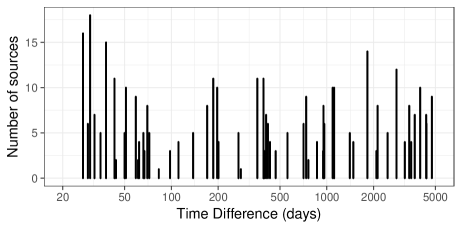
Figure 1: The separation in time between pairs of observations used to construct the sample

As our aim is to determine variability measurements that can be used to model the flux of an AGN about which nothing other than its flux and date of observation is known, we make no attempt to cross match our sample with known AGN. This means that we do not assume knowledge of the redshift of any sources; we work in terms of the observed flux and unless noted otherwise, all timescales are in the observer’s frame. This also means that, strictly speaking, we should refer to the sources we analyse as "X-ray point sources", but given our selection of fields, the point sources will be dominated by AGN, and we refer to them as AGN throughout.

2.1 Chandra data analysis

The Chandra observations were reduced and analysed using CIAO version 4.8.2 and CALDB version 4.7.2. The data were reduced following the standard procedures using the chandra_repro script, and the deflare tool to remove periods of high background.

Next, for each pair of observations the astrometry of the observations was corrected to ensure they matched closely. This is necessary, as in many cases a source will be detected in one observation but not in the other, requiring forced photometry at the source coordinates. If the two observations had a small offset in astrometry then the aperture would be offset from the source position in the observation in which the source was not detected. This would artificially reduce the inferred source flux, biasing the apparent variability to be higher than the true variability.

To perform the astrometric correction, the longer of the two observations was defined as observation 1, and the shorter as observation 2. Sources were detected in each observation in the $0.5-7\mbox{$\text{~{}keV}$}$ energy band using the CIAO wavdetect tool, and those detected with at least $7\sigma$ significance were used to register the images. Observation 2 was corrected to match the astrometry of observation 1. In all but three pairs of observations, at least 10 sources were available to register the images, with at least 6 sources used in the other three pairs. The size of the astrometric correction was typically small. The median correction was $0.3\arcsec$, and was less than $1\arcsec$ in all but three cases (the correction was smaller than $1.5\arcsec$ in those cases).

Source detection was then repeated on the corrected observations, and the source lists for a pair of observations were compared. Sources whose positions matched within $1\arcsec$ between the two observations were considered to be detections of the same source, and we refer to such a source as a "detected pair" (we demonstrate later that using a more conservative matching radius of $0.5\arcsec$ has no impact on our results). Sources detected in one observation which had no matching source within $10\arcsec$ in the other observation were considered to be undetected in the second observation, and such a source is referred to as a "detected/undetected pair". Detected sources with a position match between $1\arcsec$ and $10\arcsec$ are excluded as likely spurious matches.

Next, aperture photometry was performed using the CIAO srcflux tool in the $0.5-2\mbox{$\text{~{}keV}$}$ band. The apertures used for the source regions were circles with a radius enclosing $90\%$ of the PSF at $1.25\mbox{$\text{~{}keV}$}$. For the background region, an annulus with an inner radius equal to the source region and an outer radius five times larger was used. In the case of detected pairs, photometry was performed at the source position determined in each observation. In the case of detected/undetected pairs, forced photometry was performed in the observation without a detection at the coordinates of the detected source. Our requirement that detected/undetected pairs have no other sources within $10\arcsec$ ensures that this forced photometry does not include any contribution from a slightly offset detection of the same source or other nearby sources.

Fluxes were calculated from the inferred count rates assuming a power law spectral model with a photon index of 1.7, and were corrected for Galactic absorption (Dickey & Lockman, 1990). This analysis provided us with robust flux measurements for all sources, determined using a Bayesian method to marginalise over the background uncertainty for each source and takes into account cross-talk between the source and background regions. We use the mode of the posterior probability distribution of the flux as our estimate of the source flux, and in the case where the mode was zero we define the $1\sigma$ upper limit on the flux as the value below which $68\%$ of the probability density is contained. Note that in our analysis, these fluxes are only used for selecting subsets of sources; our likelihood calculations make use of the raw measurements of the source and background count rates, areas and exposures for each source.

At this stage we performed some additional filtering of the source list. Sources falling more than $6\arcmin$ off-axis in either observation were rejected to avoid any systematics due to the increasing PSF (the $90\%$ encircled energy fraction of the PSF is $<5\arcsec$ within this off-axis angle for the energies considered). This also eliminates cases where a source might be out of the field of view in one of the two observations. Sources flagged as near chip gaps by srcflux were excluded. We also rejected 51 sources flagged as extended by wavdetect. Finally, if a source was detected in multiple pairs of observations of the same field, only the pair with the longest interval between observations was retained, leaving a sample of 1511 unique sources, of which 767 were detected/undetected pairs.

While we use only a subset of these 1511 sources for our variability analysis, the observed properties of all sources are given in Table 2 (the table displays the first 60 sources and full table is available in the electronic version of the paper). Sources were given a unique identifier of the form $O_{1}\_O_{2}\_i$ where $O_{1}$ and $O_{2}$ are the Chandra observation identifiers for observation 1 and 2 respectively (where the longest observation is defined to be observation 1), and $i$ is an integer indicating the source number in each pair of observations.

The fluxes of the AGN in the two observations ($F_{1}$ and $F_{2}$ respectively) are plotted in Fig. 2. The sources with upper limits are shown in the centre and right panels. There are more upper limits for $F_{2}$ because observation 1 was defined to be the longer of the two. There are fewer upper limits (205 in total) than the 767 detected/undetected pairs as non-zero fluxes are measured by forced photometry in many of those cases.

The fluxes scatter about the line of equality as expected, with the scatter increasing to lower fluxes due to the increased statistical scatter. The variability in the sources is manifested in the intrinsic scatter about this line of equality. Measuring this variability relies on the correct modelling of the statistical uncertainty in the fluxes (which is non-Gaussian as most sources are in the Poisson regime), and the inclusion of upper limits. As described in the next section, this is achieved by expressing the flux variability in terms of the observed photon counts, rather than using the inferred fluxes directly.

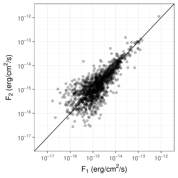
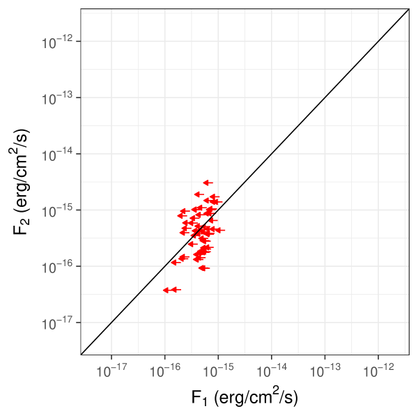
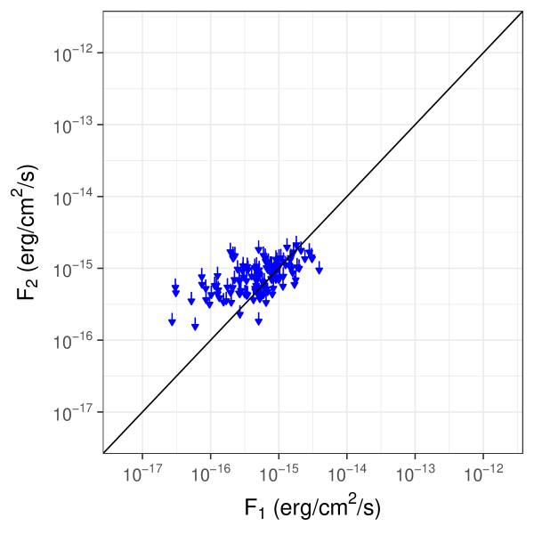
Figure 2: The fluxes of the AGN in the two observations for the full sample. Left: AGN with fluxes measured in both observations. Centre: AGN with upper limits on $F_{1}$. Right: AGN with upper limits on $F_{2}$. The solid line in each panel is a line of equality, and error bars are omitted for clarity. Upper limits are at the $1\sigma$ level.

3 The AGN variability model

In this section we will construct a likelihood function relating the characteristic variability of the AGN in a sample to the observed source and background counts. This combines the likelihood associated with the photometric measurements for a pair of fluxes, and the likelihood of a pair of fluxes given the characteristic variability. Expressed in this way, the likelihood function properly accounts for the Poisson nature of the observed counts, which naturally avoids the need to model upper limits on any inferred fluxes.

3.1 Photometric measurements

For a given AGN, the key observed quantities are the photon counts in the source and background apertures. We denote these as $T_{1},T_{2}$ in the source aperture and $B_{1},B_{2}$ in the background aperture. We wish to calculate the likelihood of observing these quantities given a set of model parameters.

We use the terms "source intensity" $s$ and "background intensity" $b$ to refer to the mean number of counts expected in a particular aperture (i.e. the mean of the Poisson distribution from which the observed counts are drawn). These are related to the corresponding fluxes, $F$ and $F_{b}$ respectively, by an energy conversion factor $\kappa$, which accounts for the instrument response, source or background spectral shape, and exposure length. This conversion factor is defined such that $F=\kappa s$, and $\kappa$ is known for each observation of each AGN.

For a particular observation of a given AGN, the observed counts in the background aperture $B$ is a Poisson realisation of the background intensity $b$. We can thus write the stochastic relation between the observed counts and background intensity as

$$P(B|b)=\text{dpois}(B|b)$$ (1)

denoting that $B$ is distributed with a Poisson probability density with mean $b$.

For the same AGN, the total counts $T$ in the source aperture contain a contribution from the source and background intensities. Thus

$$P(T|s,b,r)=\text{dpois}(T|s+b/r)$$ (2)

where $r$ accounts for the difference in detector area $A$ and effective area $E$ between the source and background apertures:

$$r=\frac{E_{b}}{E_{s}}\frac{A_{b}}{A_{s}}$$ (3)

In principle, one can also account for the fact that the PSF scatters some of the source photons into the background aperture. However, given that all apertures are defined in the same way to contain 90% of the source flux, and that we are interested in variability rather than absolute flux values, this effect can be neglected (we verified that including this effect made no significant change to our results).

The background intensity can then be marginalised over to give the joint likelihood of $T$ and $B$ for a given AGN:

$$P(T,B|s,r)=\int\text{dpois}(T|s+b/r)\text{dpois}(B|b)\,\text{d}b$$ (4)

For a pair of observations of the same AGN at different epochs, the measurements are independent and expressing the intensities in terms of fluxes (using $F=\kappa s$), the joint likelihood is

$$P(T_{1},B_{1},T_{2},B_{2}|F_{1},\kappa_{1},r_{1},F_{2},\kappa_{2},r_{2})=\\ P(T_{1},B_{1}|F_{1},\kappa_{1},r_{1})\,P(T_{2},B_{2}|F_{2},\kappa_{2},r_{2})\,.$$ (5)

One of the important features of our model is the inclusion of the Poisson likelihood to model the observed counts directly, rather than using derived fluxes and assuming Gaussian statistics. For the main sample of 416 AGN we define in §3.4, the median of the minimum net counts recorded for each AGN in its two observations is $\approx 22$ (i.e. for half of the sample, the source has $\,\hbox to0.0pt{\raise 1.72218pt\hbox{$<$}\hss}{\lower 2.58334pt\hbox{$\sim$}}\,22$ net counts in at least one of the two observations). Assuming Gaussian statistics would therefore be a poor approximation for a large fraction of the AGN.

3.2 Characteristic variability

The fundamental aim of this work is to determine the characteristic amount by which AGN vary in X-ray brightness between observations separated by months to years. Motivated by this, we model an AGN as having some mean long-term flux $F$, with some variability $\sigma$. We then assume that fluxes averaged over typical observation lengths (10s of ks) measured at epochs separated by months to years are sampled from a lognormal distribution centred on $\log(F)$ with a standard deviation $\sigma$. Working in natural log space, $\sigma$ then represents the characteristic fractional variability of the AGN on the timescales probed. We further assume that the variability of all AGN can be described by similar lognormal distributions, each with a different mean flux, but all sharing the same fractional variability $\sigma$. Our aim is then to determine the value of $\sigma$, the characteristic fractional X-ray variability of AGN between observation epochs. This assumption of log-normality is similar to many previous studies of variability in ensembles of AGN, which have measured the average fractional variability (e.g. Almaini et al., 2000; Mateos et al., 2007)

In this model, the probability distribution for a pair of fluxes $F_{1},F_{2}$ is

$$P(F_{1},F_{2}|F,\sigma)=\\ \text{dlnorm}(F_{1}|\log(F),\sigma)\,\text{dlnorm}(F_{2}|\log(F),\sigma)\,,$$ (6)

where dlnorm is the lognormal probability density function, and $\sigma$ is the quantity in which we are interested, describing the fractional variability of the AGN.

It is known a-priori that AGN fluxes are not uniformly distributed, but instead follow a distribution (generically referred to as a $\log(N)-\log(S)$ distribution) which can be approximated as a power-law or broken power-law (e.g. Hasinger et al., 1998; Mateos et al., 2008; Lehmer et al., 2012). We therefore write the prior probability density on $F$ as

$$P(F|\beta)=C(F)^{-\beta},$$ (7)

i.e. the source flux ($F$) is distributed with a power-law probability density with a negative slope $\beta$, and $C$ is a normalisation factor computed to normalise the density to unity over the range of flux considered. The slope of the $\log(N)-\log(S)$ distribution $\beta$ is a nuisance parameter in our model, but as we will see later, with a suitable sample definition our constraints on the variability are insensitive to this parameter.

The mean flux can then be marginalised over, and combining Equations Eq. 6 and 7 we then obtain

$$P(F_{1},F_{2}|\sigma,\beta)=\int P(F_{1},F_{2}|F,\sigma)P(F|\beta)\,\text{d}F\,.$$ (8)

ID	Det1	Det2	RA1	Dec1	$T_{1}$	$A_{s1}$	$E_{s1}/10^{6}$	$B_{1}$	$A_{b1}$	$E_{b1}/10^{6}$	$\kappa_{1}/10^{-15}$	$F_{1}/10^{-15}$	RA2	Dec2	$T_{2}$	$A_{s2}$	$E_{s2}/10^{6}$	$B_{2}$	$A_{b2}/10^{6}$	$E_{b2}$	$\kappa_{2}/10^{-15}$	$F_{2}/10^{-15}$	Separation	$\Delta t$
			(J2000)	(J2000)	counts	pixels	cm2 s	counts	pixels	cm2 s	$\mbox{$\text{~{}erg}$}\mbox{$\text{~{}s}$}^{-1}\mbox{$\text{~{}cm}$}^{-2}$	$\mbox{$\text{~{}erg}$}\mbox{$\text{~{}s}$}^{-1}\mbox{$\text{~{}cm}$}^{-2}$	(J2000)	(J2000)	counts	pixels	cm2 s	counts	pixels	cm2 s	$\mbox{$\text{~{}erg}$}\mbox{$\text{~{}s}$}^{-1}\mbox{$\text{~{}cm}$}^{-2}$	$\mbox{$\text{~{}erg}$}\mbox{$\text{~{}s}$}^{-1}\mbox{$\text{~{}cm}$}^{-2}$	arcsec	days
$11997\_11742\_7$	1	0	0.0658	-50.1777	6	70.1	27.1	16	1692.3	23.3	0.12	0.69	0.0658	-50.1777	0	70.1	9.2	7	1690.4	8.6	0.33	0.85†	0.0	362
$11997\_11742\_6$	1	0	0.0960	-50.1940	12	186.9	26.6	51	4503.9	26.4	0.12	1.31	0.0960	-50.1940	5	186.7	9.7	11	4499.0	9.6	0.32	1.63	0.0	362
$6105\_3261\_52$	1	0	2.8468	-15.4007	2	144.3	15.5	10	3407.5	15.1	0.20	0.35	2.8469	-15.4007	0	287.8	9.4	7	6588.8	9.6	0.33	0.85†	0.0	951
$6105\_3261\_3$	1	1	2.8820	-15.3890	231	29.6	15.7	14	712.0	14.9	0.20	52.2	2.8820	-15.3890	120	100.8	10.3	11	2328.9	10.1	0.30	40.2	0.2	951
$6105\_3261\_11$	1	1	2.8829	-15.4318	30	134.6	16.3	10	3238.0	16.3	0.19	6.4	2.8829	-15.4318	9	69.3	9.6	3	1674.6	9.5	0.32	3.13	0.4	951
$6105\_3261\_66$	0	1	2.8914	-15.4547	2	272.9	16.0	17	6561.2	16.0	0.20	0.28	2.8914	-15.4547	5	68.8	10.3	3	1655.0	10.2	0.30	1.61	0.0	951
$6105\_3261\_41$	1	0	2.9066	-15.3891	3	13.5	14.2	9	331.1	15.2	0.22	0.67	2.9066	-15.3891	4	38.4	10.4	17	927.4	10.4	0.30	1.1	0.0	951
$6105\_3261\_2$	1	1	2.9163	-15.3946	207	14.9	17.3	47	361.2	17.3	0.18	42	2.9163	-15.3946	76	23.1	10.5	22	556.6	10.5	0.29	25.2	0.2	951
$6105\_3261\_37$	1	0	2.9172	-15.4291	8	84.7	16.8	4	2040.4	16.8	0.19	1.63	2.9172	-15.4291	1	13.4	10.5	1	327.6	10.5	0.29	0.3	0.0	951
$6105\_3261\_72$	0	1	2.9179	-15.4341	2	104.2	16.8	8	2501.6	16.7	0.19	0.34	2.9179	-15.4341	3	13.5	10.5	1	338.5	10.5	0.29	0.94	0.0	951
$6105\_3261\_44$	1	0	2.9186	-15.3696	6	8.8	16.7	4	213.4	16.6	0.19	1.22	2.9186	-15.3696	2	60.8	10.2	28	1467.6	10.2	0.31	0.29	0.0	951
$6105\_3261\_54$	1	0	2.9204	-15.3499	2	9.5	16.5	0	233.8	15.9	0.19	0.37	2.9204	-15.3500	1	126.5	10.1	11	3051.6	9.9	0.31	0.18	0.0	951
$6105\_3261\_35$	1	0	2.9205	-15.4006	12	20.1	17.3	21	481.9	17.2	0.18	2.25	2.9206	-15.4006	3	15.6	10.5	8	380.5	10.5	0.29	0.89	0.0	951
$6105\_3261\_30$	1	1	2.9253	-15.3680	2	8.9	17.4	2	215.3	17.4	0.18	0.38	2.9253	-15.3681	42	57.2	9.2	3	1375.1	9.0	0.33	14.9	0.5	951
$6105\_3261\_12$	1	1	2.9286	-15.4309	29	92.6	15.2	11	2224.4	15.7	0.22	6.91	2.9286	-15.4309	14	10.1	10.5	3	248.2	10.5	0.29	4.44	0.2	951
$6105\_3261\_67$	0	1	2.9409	-15.4454	2	168.6	16.6	17	4054.9	16.6	0.19	0.27	2.9409	-15.4454	0	11.7	9.9	5	2659.5	9.2	0.30	0.77†	0.0	951
$6105\_3261\_4$	1	1	2.9475	-15.3888	61	18.5	17.5	14	447.8	17.5	0.18	12.2	2.9475	-15.3889	8	15.4	10.4	8	379.6	10.4	0.30	2.6	0.2	951
$6105\_3261\_6$	1	1	2.9491	-15.3742	72	13.2	17.4	10	319.9	17.4	0.18	14.9	2.9491	-15.3743	24	32.4	8.9	3	790.0	9.1	0.36	9.33	0.1	951
$6105\_3261\_65$	0	1	2.9498	-15.3784	5	14.5	17.5	8	349.5	17.5	0.18	0.94	2.9498	-15.3784	4	27.2	9.5	6	658.1	9.5	0.32	1.35	0.0	951
$6105\_3261\_1$	1	1	2.9506	-15.4154	40	61.7	17.2	11	1487.4	17.2	0.18	8.12	2.9506	-15.4154	12	8.8	10.4	7	213.6	10.4	0.29	3.87	0.3	951
$6105\_3261\_51$	1	0	2.9538	-15.4039	3	39.6	17.3	11	955.4	17.3	0.18	0.51	2.9538	-15.4039	0	9.9	10.4	2	241.4	10.3	0.29	0.76†	0.0	951
$6105\_3261\_7$	1	1	2.9711	-15.3649	25	32.1	16.1	6	775.2	14.4	0.19	5.41	2.9711	-15.3649	12	68.8	10.0	7	1654.0	10.0	0.31	4.06	0.1	951
$6105\_3261\_62$	0	1	2.9735	-15.4447	1	267.1	16.4	18	6418.3	16.4	0.19	0.05	2.9735	-15.4447	2	17.5	10.4	0	427.2	10.4	0.29	0.58	0.0	951
$15173\_904\_17$	1	1	10.3600	-9.3700	53	85.6	14.9	67	2070.4	14.7	0.23	12.9	10.3600	-9.3700	76	146.9	17.2	132	3547.4	17.1	0.17	13.9	0.3	4743
$15173\_904\_36$	1	0	10.3739	-9.4157	4	199.7	14.8	67	4796.5	14.6	0.23	0.31	10.3739	-9.4157	4	140.6	18.4	78	3373.9	18.0	0.17	0.14	0.0	4743
$15173\_904\_45$	0	1	10.3952	-9.4342	2	279.4	16.0	94	6708.9	15.8	0.21	0.80†	10.3952	-9.4342	10	125.9	18.7	58	3035.3	18.4	0.16	1.39	0.0	4743
$15173\_904\_7$	1	1	10.3955	-9.3358	15	12.9	15.9	18	310.5	16.3	0.21	3.29	10.3954	-9.3357	19	62.8	18.6	97	1519.6	18.2	0.16	2.68	0.2	4743
$15173\_904\_20$	1	1	10.4020	-9.3232	7	13.2	15.9	23	320.0	15.6	0.21	1.44	10.4020	-9.3231	16	77.0	18.9	143	1854.1	18.5	0.16	1.76	0.3	4743
$15173\_904\_1$	1	1	10.4021	-9.3943	27	53.0	17.0	32	1278.2	17.0	0.20	5.77	10.4021	-9.3943	40	28.7	19.1	22	688.5	18.0	0.16	6.95	0.7	4743
$15173\_904\_2$	1	1	10.4159	-9.3883	23	32.4	17.2	34	778.1	17.2	0.20	4.82	10.4159	-9.3883	32	14.1	18.7	20	343.5	18.6	0.16	5.91	0.3	4743
$15173\_904\_5$	1	1	10.4195	-9.3556	53	9.1	17.5	28	224.1	17.5	0.19	11.4	10.4195	-9.3556	73	15.2	19.6	47	370.8	19.4	0.15	12.3	0.3	4743
$15173\_904\_48$	0	1	10.4584	-9.3533	5	20.6	17.6	72	501.4	17.6	0.19	0.45	10.4584	-9.3533	11	12.7	17.5	41	305.1	16.8	0.17	1.83	0.0	4743
$15173\_904\_55$	0	1	10.4697	-9.3364	7	31.5	16.5	146	756.9	16.5	0.21	0.21	10.4697	-9.3364	19	29.6	19.3	214	712.9	19.3	0.16	1.79	0.0	4743
$15173\_904\_11$	1	1	10.4718	-9.4185	29	229.5	14.7	152	5513.4	14.9	0.23	5.96	10.4718	-9.4186	27	40.8	15.9	29	992.5	17.3	0.19	5.55	0.6	4743
$15173\_904\_15$	1	1	10.4748	-9.3792	17	78.9	16.2	126	1895.9	16.2	0.21	2.78	10.4748	-9.3792	19	14.5	19.8	35	348.9	19.8	0.15	3.05	0.3	4743
$15173\_904\_13$	1	1	10.4893	-9.4113	87	273.6	16.4	151	6517.5	15.9	0.21	18.9	10.4893	-9.4113	121	57.6	19.5	46	1389.2	19.0	0.16	20.9	0.1	4743
$15173\_904\_49$	0	1	10.5063	-9.3335	21	156.0	14.3	359	3750.4	15.1	0.24	1.61	10.5063	-9.3335	39	109.0	15.1	283	2615.1	17.1	0.20	6.17	0.0	4743
$15173\_904\_43$	1	0	10.5184	-9.3308	29	254.1	15.2	406	6118.1	15.4	0.23	3.07	10.5185	-9.3308	11	167.9	15.4	334	4036.9	16.8	0.19	1.21†	0.0	4743
$13458\_3233\_62$	1	0	13.8713	26.4314	16	203.9	42.3	41	4894.6	40.7	0.08	1.34	13.8712	26.4314	1	72.6	23.6	4	1743.6	23.6	0.14	0.12	0.0	3682
$13458\_3233\_15$	1	1	13.8797	26.4147	129	111.8	45.9	26	2712.6	44.3	0.08	11.1	13.8797	26.4147	78	44.3	22.2	8	1068.6	21.1	0.14	12.5	0.2	3682
$13458\_3233\_61$	1	0	13.8843	26.3699	5	69.3	42.7	12	1674.6	43.6	0.08	0.41	13.8843	26.3699	6	80.3	20.3	11	1930.1	19.9	0.16	0.98	0.0	3682
$13458\_3233\_75$	0	1	13.8903	26.4538	2	232.2	44.5	66	5366.0	42.6	0.08	0.32†	13.8902	26.4538	5	59.8	16.6	10	1437.6	19.6	0.20	1.01	0.0	3682
$13458\_3233\_26$	1	1	13.8936	26.4553	20	228.3	45.7	70	5246.9	44.6	0.08	1.48	13.8935	26.4553	5	57.1	20.5	5	1364.7	19.3	0.16	0.84	0.3	3682
$13458\_3233\_23$	1	1	13.8964	26.4329	7	109.8	43.6	31	2639.4	43.2	0.08	0.52	13.8964	26.4329	3	27.1	24.1	2	653.4	23.8	0.13	0.43	0.7	3682
$13458\_3233\_70$	0	1	13.9046	26.4086	0	41.5	46.6	20	998.5	45.4	0.07	0.19†	13.9046	26.4086	1	16.4	22.5	1	399.6	22.2	0.14	0.15	0.0	3682
$13458\_3233\_4$	1	1	13.9049	26.3563	35	34.6	43.4	24	836.0	43.8	0.08	3.03	13.9049	26.3562	20	77.5	22.4	12	1863.1	21.9	0.14	3.08	0.4	3682
$13458\_3233\_59$	1	0	13.9130	26.4648	11	226.8	41.1	74	5454.7	40.7	0.09	0.78	13.9130	26.4648	2	51.2	23.6	10	1232.0	23.6	0.14	0.24	0.0	3682
$13458\_3233\_11$	1	1	13.9151	26.3972	11	20.9	41.4	10	508.5	39.7	0.08	0.98	13.9151	26.3972	6	13.5	24.0	7	340.8	24.0	0.13	0.88	0.2	3682
$13458\_3233\_1$	1	1	13.9202	26.3410	24	33.8	44.5	9	815.0	45.9	0.08	2.02	13.9202	26.3410	12	113.6	21.1	22	2732.8	21.5	0.15	1.84	0.4	3682
$13458\_3233\_50$	1	0	13.9396	26.3687	8	10.1	48.9	9	244.6	48.9	0.07	0.6	13.9396	26.3687	2	27.3	19.4	7	677.5	20.2	0.17	0.32	0.0	3682
$13458\_3233\_3$	1	1	13.9402	26.3544	31	14.4	48.7	15	346.5	48.7	0.07	2.47	13.9402	26.3543	23	58.4	22.8	17	1405.5	22.8	0.14	3.59	0.4	3682
$13458\_3233\_12$	1	1	13.9427	26.3988	34	10.2	49.3	9	249.0	48.8	0.07	2.62	13.9427	26.3988	15	9.1	24.0	9	228.4	24.0	0.14	2.29	0.2	3682
$13458\_3233\_29$	1	1	13.9448	26.4634	12	160.4	43.1	64	3846.6	43.8	0.08	0.88	13.9448	26.4634	12	34.9	23.9	11	848.8	23.3	0.14	1.79	0.7	3682
$13458\_3233\_10$	1	1	13.9588	26.3948	27	9.1	48.9	10	225.7	48.7	0.07	2.17	13.9588	26.3948	20	11.3	24.0	17	275.3	24.0	0.14	3.12	0.1	3682
$13458\_3233\_44$	1	1	13.9597	26.4698	15	209.4	44.2	59	5031.1	44.3	0.08	1.13	13.9597	26.4698	3	58.1	23.8	7	1397.1	23.1	0.14	0.41	0.3	3682
$13458\_3233\_51$	1	0	13.9654	26.4275	38	33.2	48.8	194	799.7	48.7	0.07	2.44	13.9654	26.4275	3	11.9	24.1	39	290.7	24.1	0.14	0.21	0.0	3682
$13458\_3233\_54$	1	0	13.9662	26.3230	33	54.9	42.9	106	1320.2	44.8	0.08	2.58	13.9662	26.3229	19	241.8	19.6	218	5797.9	20.6	0.17	1.87	0.0	3682
$13458\_3233\_73$	0	1	13.9718	26.4691	7	215.8	42.4	61	5187.9	44.1	0.08	0.41	13.9718	26.4692	3	68.9	23.8	14	1661.4	23.0	0.14	0.37	0.0	3682
$13458\_3233\_55$	1	0	13.9860	26.3771	22	13.4	48.4	32	327.6	48.4	0.07	1.72	13.9860	26.3771	7	47.8	23.4	35	1155.1	23.4	0.14	0.89	0.0	3682
$13458\_3233\_9$	1	1	13.9866	26.3903	8	14.5	48.5	39	349.7	48.4	0.07	0.52	13.9866	26.3903	4	32.1	23.8	42	775.7	23.8	0.14	0.35	1.0	3682

Table 2: Properties of the detected sources. ID is a unique identifier of each source of the form $O1\_O2\_I$ where $O1$ and $O2$ are the Chandra observation identifiers for observation 1 and 2 respectively, and $I$ is an integer indicating the source number in each pair of observations. Observation 1 is defined to be the longer of the two observations. For the other columns, subscripts 1 and 2 indicate whether the quantity is measured for observation 1 or 2, and subscripts $s$ and $b$ indicate if the quantity is measured for the source or background region, respectively. "Det" is a binary flag indicating whether a source was detected in a given observation (if not then forced photometry was performed at the source position determined from the other observation). RA and Dec give the source coordinates in degrees. $T$ gives the total number of counts in the source region, $A$ gives the area of each region in pixels ($0.492\arcsec$ on a side), $E$ gives the mean exposure map value in each region, $B$ gives the total counts in the background region, and $\kappa$ gives the energy conversion factor for the source. $F$ is the unabsorbed flux of the source, determined from the mode of the posterior probability distribution of the flux, where values marked with $\dagger$ are $1\sigma$ upper limits. The "Separation" column gives the angular separation between detections of the same source in the two observations, and $\Delta t$ gives the separation in days between the two observations. All photometric quanities are measured in the $0.5-2\mbox{$\text{~{}keV}$}$ band in the observer’s frame. This is a truncated version of the table; the full data for all 1511 sources are presented in the online version of the paper.

3.3 The final likelihood

The likelihood of the counts observed in a pair of observations of an AGN, given $\sigma$ and $\beta$ can now be written by combining equations 5 and 8 and marginalising out $F_{1}$ and $F_{2}$ to give

$$P(T_{1},B_{1},T_{2},B_{2}|\sigma,\beta,\kappa_{1},r_{1},\kappa_{2},r_{2})=\\ \int\int P(T_{1},B_{1},T_{2},B_{2}|F_{1},\kappa_{1},r_{1},F_{2},\kappa_{2},r_{2})\times\\ P(F_{1},F_{2}|\sigma,\beta)\,\text{d}F_{1}\,\text{d}F_{2}$$ (9)

The final likelihood for a sample of $N$ AGN is the product of the individual probabilities:

$${\cal L}=\prod_{i=1}^{N}P(T_{1,i},B_{1,i},T_{2,i},B_{2,i}|\sigma,\beta,\kappa_{1,i},r_{1,i},\kappa_{2,i},r_{2,i})$$ (10)

In principle one could multiply this likelihood by priors on $\sigma$ and $\beta$ and treat it as a posterior distribution to be sampled with standard Bayesian techniques. However, evaluating this likelihood function for a sample size of a few hundred AGN is computationally expensive due primarily to the Poisson probability evaluations inside nested integrals. This can be mitigated by splitting the sources over multiple CPU cores to evaluate their likelihoods in parallel and combining these for final likelihood. Even so, for a typical fit of $\sim 300$ AGN spread across 30 CPU cores (using more cores leads to diminishing returns due to overheads), each likelihood evaluation took around $20\mbox{$\text{~{}s}$}$ of wall time. For this reason we adopted a simple maximum-likelihood analysis, and given the model has just two parameters (or one when $\beta$ is fixed), straightforward grid searches were sufficient to map the likelihood distribution.

Parameter uncertainties were estimated using the likelihood ratio method (e.g. Cash, 1979), noting that $2\log{{\cal L}}$ is $\chi^{2}$ distributed with a number of degrees of freedom equal to the number of model parameters. Thus for a two parameter fit the $(1\sigma,2\sigma,3\sigma)$ confidence intervals enclose the parameter values for which $2\log{{\cal L}_{0}}-2\log{{\cal L}}>(2.3,6.0,11.6)$, where ${\cal L}_{0}$ is the maximum value of the likelihood. For a single parameter fit, the corresponding levels are $2\log{{\cal L}_{0}}-2\log{{\cal L}}>(0.98,3.8,8.8)$.

3.4 Subsample definition and selection biases

The selection of the sample used for this type of ensemble variability analysis can easily result in biases that will increase or decrease the apparent value of $\sigma$. With no additional selection applied, our sample of AGN is defined by the requirement that each AGN be detected by wavdetect in at least one of its two observations. In principle this selection function could be modelled with simulations but it is possible instead to define a subsample for which the selection results in an unbiased estimate of $\sigma$.

As an illustration, consider samples defined using a limit in the observed flux $F_{\text{lim}}$. One could define a sample of the AGN for which ($F_{1}>F_{\text{lim}})\text{ OR }(F_{2}>F_{\text{lim}})$. This is illustrated in the left panel of Fig. 3 and as is apparent, this selection results in an overestimate of $\sigma$ due to the exclusion of AGN with small flux differences near $F_{\text{lim}}$. An alternative selection of $(F_{1}>F_{\text{lim}})\text{ AND }(F_{2}>F_{\text{lim}})$ is illustrated in the central panel of Fig. 3. This is illustrative of a sample where the source is required to be detected in all observations (for example in a source catalogue). In this case $\sigma$ will be underestimated due to the exclusion of AGN with large flux differences close to $F_{\text{lim}}$. In both cases, the slope $\beta$ of the population distribution influences the amount of bias on $\sigma$ since increasing $\beta$ increases the density of AGN close to $F_{\text{lim}}$, whence the bias originates.

The selection bias and dependence on $\beta$ can be avoided entirely by defining a sample with a flux selection that is orthogonal to the line of equality of the two fluxes. Since $\sigma$ is measured in log space, this selection must also be made in log space, and corresponds to $\sqrt{F_{1}F_{2}}>F_{\text{lim}}$ (i.e. the geometric mean of the two fluxes is greater than $F_{\text{lim}}$). This is illustrated in the right panel of Fig 3, and all of the samples used in our analysis are defined in this way.

Even using this geometric mean flux limit, one possible source of bias remains. If $F_{\text{lim}}$ were set too low, then the sample would begin to include false positive sources. Including these sources would bias $\sigma$ high, since they would be associated with a background noise peak in one image and a random background value in the other image. To minimise this, we set the flux limit to $F_{\text{lim}}=2.5\times 10^{-15}\mbox{$\text{~{}erg}$}\mbox{$\text{~{}s}$}^{-1}\mbox{$\text{~{}cm}$}^{-2}$. This limits the sample to 416 sources of which 408 were detected with a significance $>3\sigma$ in at least one observation (the remaining 8 were all detected at $>2.4\sigma$ in at least one observation), leading to a highly pure sample.

When computing the geometric mean fluxes for subsample selections, we used the fluxes measured with srcflux. The mode of the flux posterior was used for most sources, but in the case of upper limits (when the mode is zero), the value of the flux upper limit was used instead. However, no such sources with a flux upper limit exceeded the flux limits used to define the subsamples for our analysis, so none were ultimately included in the variability measurements.

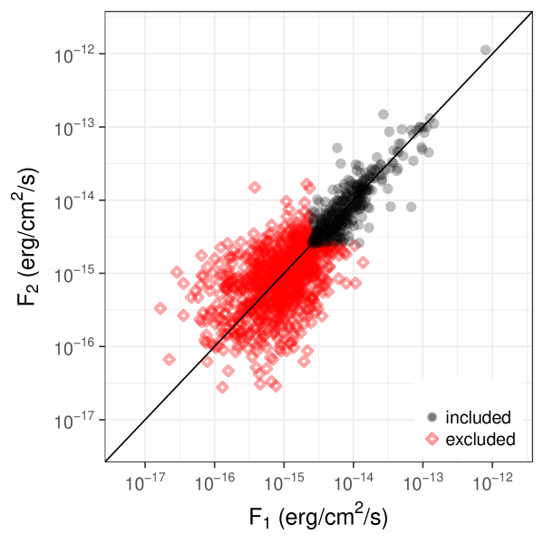
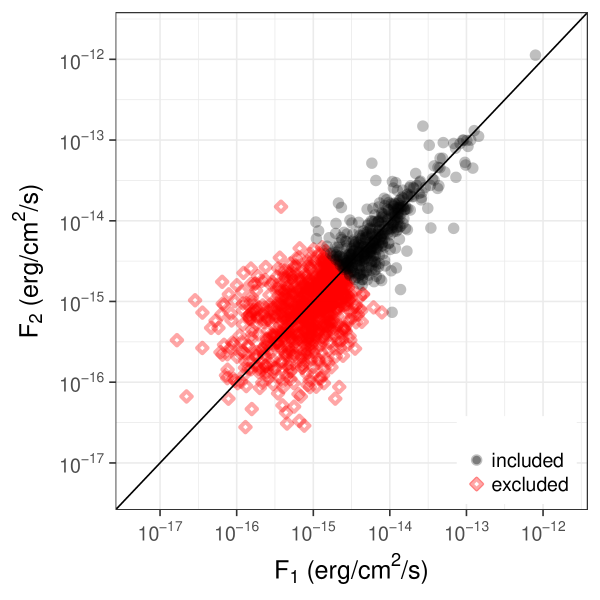
Figure 3: Illustration of sample definitions and resulting biases. The points show the measured fluxes in each observation for the full sample, excluding error bars and upper limits for clarity. Filled circles indicate points included by a given sample definition while hollow diamonds indicate excluded points. The left panel illustrates a selection where $(F_{1}\text{ OR }F_{2})>2.5\times 10^{-15}\mbox{$\text{~{}erg}$}\mbox{$\text{~{}s}$}^{-1}\mbox{$\text{~{}cm}$}^{-2}$, which biases the measured $\sigma$ high. The centre panel illustrates a selection where $(F_{1}\text{ AND }F_{2})>2.5\times 10^{-15}\mbox{$\text{~{}erg}$}\mbox{$\text{~{}s}$}^{-1}\mbox{$\text{~{}cm}$}^{-2}$ (biasing the measured $\sigma$ low). The right panel illustrates a selection where $\sqrt{F_{1}F_{2}}>2.5\times 10^{-15}\mbox{$\text{~{}erg}$}\mbox{$\text{~{}s}$}^{-1}\mbox{$\text{~{}cm}$}^{-2}$, which imposes no bias on $\sigma$.

4 Results

We obtained our main results by considering a subsample of AGN for which the two observations were separated by at least a year, to reduce sensitivity to short-term variability. This subsample contained 222 AGN, of which 11 were in detected/undetected pairs. We refer to this as the primary sample.

The likelihood in Eq. (9) was computed over the parameter space of $\sigma$ and $\beta$ for the primary sample, and the resulting constraints are shown in Fig. 4. The best fitting values were $\sigma=0.43\pm 0.04$ and $\beta=1.24\pm 0.02$.

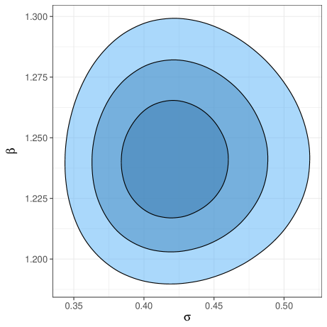
Figure 4: Constraints on AGN variability $\sigma$ and $\log(N)-\log(S)$ slope $\beta$ from the primary sample. The shaded regions enclose the $1\sigma$, $2\sigma$ and $3\sigma$ confidence intervals on the parameters.

The constraints on the two parameters are essentially independent with no degeneracy. For this reason, we fix $\beta=1.24$ for all subsequent fits in order to speed up the fitting process. (We will show in §5.1 that this has no impact on the results.) With $\beta$ fixed, the constraint on $\sigma$ for one free parameter was $\sigma=0.43\pm 0.03$. The results obtained for this and the subsequent subsamples are summarised in Table 3.

Table 3: AGN variability for different subsets of AGN. In all cases, the minimum interval between observations was one year. The first column the allowed range in separation between the sources in the two observations. The second column is the threshold in exposure time that must be exceeded by at least one of the observations. The third column gives the allowed range of the geometric mean flux of the two observations. The fourth column gives the number of AGN in the resulting subsample and the final column gives the constraints on $\sigma$. For all fits, $\beta$ was fixed at a value of 1.24.

Separation	Exposure	$\sqrt{F_{1}F_{2}}$	N	$\sigma$
(arcsec)	(ks)	$(10^{-15}\mbox{$\text{~{}erg}$}\mbox{$\text{~{}s}$}^{-1}\mbox{$\text{~{}cm}$}^{-2})$
$<1$	$>20$	$>2.5$	222	$0.43\pm 0.03$
$<0.5$	$>20$	$>2.5$	160	$0.42\pm 0.03$
$0.5-1$	$>20$	$>2.5$	62	$0.45\pm 0.05$
$<1$	$>85$	$1.0-2.5$	64	$0.53\pm 0.07$

In order to test the effect of the matching radius on the measured variability, we restricted the sample to the 165 AGN in the primary sample with a matching radius of $<0.5\arcsec$. For this subset, the best fitting variability was $\sigma=0.42\pm 0.03$, fully consistent with the previous measurement. Meanwhile, for the 65 AGN with matching radii between $0.5\arcsec$ and $1\arcsec$, the variability was $\sigma=0.45\pm 0.05$. We thus conclude that using a $1\arcsec$ matching radius has no impact on our results.

Finally, we also investigated if there was evidence for $\sigma$ being different for lower flux AGN. To do this we selected AGN for which at least one of the two observations had an exposure of at least $85\mbox{$\text{~{}ks}$}$ (chosen to give a reasonable number of deep pointings). We then selected sources with geometric mean fluxes of between $1\times 10^{-15}\mbox{$\text{~{}erg}$}\mbox{$\text{~{}s}$}^{-1}\mbox{$\text{~{}cm}$}^{-2}$ and $2.5\times 10^{-15}$ to give a low-flux sample of 64 AGN (all but one detected at $3\sigma$) that had no overlap with the primary sample. For this low-flux subsample, the best fitting variability was $\sigma=0.53\pm 0.07$. This is not a very significant difference from the value of $\sigma=0.43\pm 0.03$ measured for the higher flux sources, but could be indicative of a larger variability at lower fluxes.

4.1 Variability on different timescales

Next, we measured the variability as a function of the (observer’s frame) time difference $\Delta t$ between observational epochs. For this we used the same flux selection as the primary sample, but defined five subsamples of AGN with ranges in $\Delta t$ chosen to give approximately equal numbers of AGN in each subsample. The subsamples were then modelled as before to determine the characteristic flux variability on those different timescales. The resulting constraints on $\sigma$ are shown in Table 4 and plotted in Fig. 5. Also shown in Fig. 5 is the trend of variability with rest frame time interval inferred from the structure function analysis of a large sample of AGN in Vagnetti et al. (2016). This comparison is discussed in §5.3.

Table 4: AGN variability for subsets of observations separated by different intervals in the observer’s frame. The first column gives the range in intervals between observations and the second gives the median value. The third column gives the number of AGN in the resulting subsample and the final column gives the constraints on $\sigma$. For all fits, $\beta$ was fixed at a value of 1.24.

$\Delta t$	Median $\Delta t$	N	$\sigma$
(days)	(days)
$27-51$	35	95	$0.25\pm 0.03$
$59-291$	124	88	$0.22\pm 0.03$
$357-737$	407	75	$0.42\pm 0.04$
$761-2085$	1114	78	$0.37\pm 0.04$
$2123-4743$	3490	80	$0.46\pm 0.05$

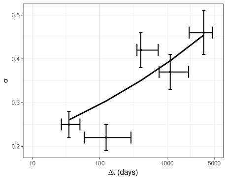
Figure 5: Constraints on AGN variability $\sigma$ for subsamples grouped by the interval between observations $\Delta t$ in the observer’s frame. The horizontal bars span the range of $\Delta t$ in each subsample with the point marking the median $\Delta t$ for each subsample. The solid line shows the variability as a function of rest frame time interval inferred from the structure function measurements of Vagnetti et al. (2016).

5 Discussion

5.1 Verification of methodology

Our AGN variability model was tested on simulated data in order to verify that the variability could be recovered accurately. A synthetic dataset was generated by sampling a large number of fluxes from a reference $\log(N)-\log(S)$ distribution, with each representing the mean flux of a different synthetic source. The variability of each synthetic source was then modelled as a lognormal distribution with the mean flux for that source and with a constant value of $\sigma$ common to all sources. For each synthetic source, a pair of fluxes were then sampled from its lognormal distribution to represent two observations of that flux. For each pair of fluxes a random real source was chosen from the list of all sources detected in our Chandra data (i.e. prior to any filtering), and the pair of synthetic fluxes were assigned the source and background areas, exposures, effective areas and background counts of the two observations of the real source. Finally, these properties were used to compute the total intensity in the source aperture for each source, and the total and background counts for each source were then sampled from Poisson distributions with the appropriate rates. This method produced a large number of synthetic observations of a realistic population of AGN with observational characteristics the represent the range of data quality in the real data.

Following this method, mock samples could be generated with different characteristics and different selection functions applied to test our model. In all cases, when the geometric mean flux selection was used, the input variability was recovered accurately. For example, we generated a population of AGN following the $0.5-2\mbox{$\text{~{}keV}$}$, broken power-law $\log(N)-\log(S)$ distribution of Lehmer et al. (2012), with slopes $\beta_{1}=1.49$ and $\beta_{2}=2.48$ at fluxes below and above $6\times 10^{-15}\mbox{$\text{~{}erg}$}\mbox{$\text{~{}s}$}^{-1}\mbox{$\text{~{}cm}$}^{-2}$ respectively. The geometric mean flux limit of $\sqrt{F_{1}F_{2}}>2.5\times 10^{-15}\mbox{$\text{~{}erg}$}\mbox{$\text{~{}s}$}^{-1}\mbox{$\text{~{}cm}$}^{-2}$ was then applied to this synthetic sample and a random subset of 1000 pairs of synthetic observations was selected. We then modelled this using the methodology used for our main results, with $\beta$ fixed at 1.24, and fitting only for $\sigma$. For an input variability of $\sigma=0.5$ our method recovered $\sigma=0.50\pm 0.02$. This demonstrates that our method is robust, and due to the geometric mean selection, is insensitive to the modelling of the $\log(N)-\log(S)$ distribution.

In the cases where the OR or AND sample selections discussed above were applied to the synthetic data, the recovered $\sigma$ was biased by $\approx 15\%$ high and low respectively.

5.2 Evaluation of our model

In the previous section we demonstrated that our model can accurately recover the true variability of realistic synthetic data. In this section we assess how well our model describes the observed data. To do this, we computed the ratio of the observed fluxes for each source in the primary sample ($F_{1}/F_{2}$). These are plotted in Fig. 6, and form the basis of a quantitative comparison with our model.

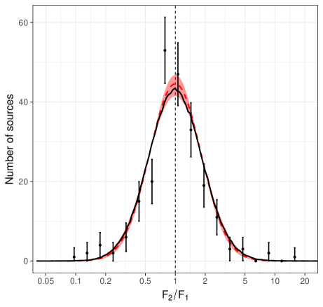
Figure 6: The distribution of the ratios of the observed fluxes for the primary sample are compared with the best fitting model. The data points show the number of sources in bins of flux ratio of constant width. The error bars show the Poisson uncertainty on the number of sources in each bin, using the Gaussian approximation of Gehrels (1986). The solid black line shows the distribution of flux ratios derived from a synthetic sample of sources generated from our best fitting model. The dashed red line and shaded $1\sigma$ error envelope show the lognormal distribution with the best fitting variability of $\sigma=0.43\pm 0.03$ multiplied by a factor of $\sqrt{2}$. As discussed in the text, this factor accounts for the uncertainty on the mean of a pair of observations. The small difference between the two curves is due to the inclusion of statistical noise and sample selection effects in the curve derived from the synthetic sample.

According to our model, the two observations of an AGN have fluxes $F_{1},F_{2}$ that are drawn from a lognormal distribution with a given $\sigma$ ($\sigma=0.43$ in the case of the primary sample). If the mean, $\log(F)$, of the distribution were known, then the ratio of $F_{1}/F$ or $F_{2}/F$ would be lognormally distributed with a mean of one and standard deviation $\sigma$. However, the ratio of pairs of independent measurements $F_{2}/F_{1}$ will be lognormally distributed with a mean of one but with a standard deviation of $\sqrt{2}\sigma$. As expanded upon in the next section, the $\sqrt{2}$ factor arises as $F_{1}$ and $F_{2}$ are both independent samples from the flux distribution. This model is plotted in Fig. 6, and appears to be a very good description of the data.

However, with this analytic form we neglect the photon counting noise on the individual flux measures, which would broaden out the distribution of flux ratios compared to the lognormal model. To model this effect we generated $10^{6}$ synthetic pairs of observations of AGN following the method of §5.1, but using the best fitting model to our primary subsample (i.e. $\sigma=0.43$, and a single power-law $\log(N)-\log(S)$ with $\beta=1.24$). The geometric mean flux limit of $\sqrt{F_{1}F_{2}}>2.5\times 10^{-15}\mbox{$\text{~{}erg}$}\mbox{$\text{~{}s}$}^{-1}\mbox{$\text{~{}cm}$}^{-2}$ was then applied to this synthetic data to match the primary sample selection, and the ratios of $F_{1}/F_{2}$ were computed for each AGN.

The distribution of flux ratios predicted by the best fitting model is plotted in Fig. 6. As expected, this is slightly broadened compared with the intrinsic lognormal distribution. Visually there is a good agreement with the observed flux ratios in this binned representation. The unbinned distribution of observed flux ratios was compared with that of the synthetic sample from the best fitting model using a two-sided Kolmogorov-Smirnov test. This gave a p value of 0.74, meaning that the data cannot rule out the null hypothesis that both the observed and synthetic samples are drawn from the same parent distribution. We thus conclude that our model is a good description of the data.

5.3 Comparison with other work

Our analysis is quite distinct from previous work on the long term variability of AGN, in that it is not focussed at understanding the intrinsic properties of the AGN, but instead on equipping the observer with the knowledge needed to mitigate their impact on other targets of interest. As such we work exclusively in the observer’s frame rather than the rest frame of the source, and do not separate out AGN into samples by redshift or luminosity.

Our analysis method has some advantages over other work. Firstly, we define a sample selection that avoids the biases introduced when applying an independent selection threshold to each observation. Secondly, we use the Poisson likelihood of the observed counts, which removes the approximation of Gaussian statistics and naturally includes non-detections and upper limits.

In the literature, two main approaches have been used to measure the characteristic variability of samples of AGN: the normalised excess variance (NXS) and the structure function (SF). Both quantities are defined precisely in Vagnetti et al. (2016) but they can be described as follows. The NXS is the variance of the flux distribution of a particular source once measurement errors have been subtracted, normalised to the mean flux of that source. The SF is the root mean square of the difference in log flux between pairs of observations, where the average is taken over sources with approximately the same time interval between observations, and the average statistical noise is subtracted.

Almaini et al. (2000) used a variation on the NXS method to measure the variability in 86 quasars on timescales of up to 14 days. Their method is not directly comparable as they utilised 16-26 flux measurements per source, spread over the 14 day period, but the average variability of $\approx 20\%$ that they found is similar to the value we find for the shortest time intervals we sampled.

Mateos et al. (2007) used the same approach as Almaini et al. (2000) to measure variability in AGN observed in 16 observations of the Lockman Hole field with XMM-Newton spread over 2 years. The average fractional variability for that sample was $0.22\pm 0.01$, which is smaller than the values of $\approx 0.4$ that we find on timescales longer than about a year. However, once again a direct comparison is difficult as the Mateos et al. (2007) measurement comes from multiple fluxes spread over 2 years while ours comes from flux pairs separated by a given interval. The mean interval between observations for the Mateos et al. (2007) value was about 40 days, so a better comparison may be with the $\approx 25\%$ variability we find on that timescale.

Vagnetti et al. (2016) investigated the variability in a sample of 2700 AGN observed multiple times with XMM-Newton, and with known redshifts using both the NXS and SF methods. Their SF measurements are quite comparable with our measurement of characteristic variability as they are determined from pairs of fluxes separated by $\Delta t$, and we thus convert their SF to a fractional variability using their equation 6.

The resulting trend in fractional variability with observation interval for the whole Vagnetti et al. (2016) sample is shown in Fig. 5, and the agreement with our measurements is very good. This is despite some significant differences between these works. In particular, the sample definition of Vagnetti et al. (2016) requires the sources to be detected in all observations, which should lead to an underestimate of the true variability, while our analysis uses the observation interval in the observer’s frame. The latter effect would blur out pairs of observations with the same rest frame interval into a range of observer’s frame intervals, flattening the slope of any trend between $\sigma$ and $\Delta t$. The good agreement between the two sets of results suggests that neither of these effects are large.

Overall, we conclude that while previous measurements using the NXS method are not directly comparable, the agreement with our results seems reasonable. The closest comparison is with the SF measurements of Vagnetti et al. (2016), where the agreement is very good.

5.4 Forecasting fluxes

We are now in a position to answer the question posed in this paper. Given a measurement of the X-ray flux $F_{1}$ of an AGN at one epoch, and with no additional knowledge of its properties, what is our best estimate of the flux $F_{2}$ at a second epoch some years earlier or later? Under these circumstances, neglecting Eddington bias (see below), the flux is equally likely to be higher or lower in the second observation, so our best estimate must be $F_{2}=F_{1}$, but the uncertainty on this depends on the variability of the source. (Of course the uncertainty also depends on the statistical noise on each observation, but we disregard that here to focus on the irreducible uncertainty due to variability.)

Consider an AGN that has a lognormal variability of its flux about a mean flux $\log(F)$, with standard deviation $\sigma$. In this case, given $N$ observations of the source with fluxes $F_{i}$, we estimate $\log(F)$ as the mean of the $\log(F_{i})$ with a precision of $\sigma/\sqrt{N}$. In other words, the probability density for $F$ is

$$P(F|F_{i},\sigma)=\text{dlnorm}(\left<\log(F_{i})\right>,\sigma/\sqrt{N}).$$ (11)

Now, to predict the flux $F^{\prime}$ of this source at the epoch of another observation, we have to marginalise out the unknown mean $F$ for which we know the posterior from the previous $N$ measurements of the flux.

$$P(F^{\prime}|F_{i},\sigma)=\int P(F^{\prime}|F,\sigma)P(F|F_{i},\sigma)\,\text{d}F$$ (12)

where both of the probabilities on the right hand side are lognormal. This results in a posterior for $F^{\prime}$ that is also lognormal, with standard deviation

$$\sigma^{\prime} =\sqrt{\sigma^{2}+\sigma^{2}/N}=\sigma\sqrt{1+\frac{1}{N}}$$ (13)

Thus, for a source with one previous flux measurement $F_{1}$ we predict the flux at a second epoch to be $F_{2}=F_{1}$ with an uncertainty on $\log(F_{2})$ of $\sigma^{\prime}=\sqrt{2}\sigma$, as above. For example, based on the $\sigma=0.43$ we found for the primary sample, for observations separated by about $1-10$ years the uncertainty on a flux prediction based on a single previous measurement is $0.43\times\sqrt{2}$ or approximately $60\%$.

In the limit of a large number of previous flux measurements, the uncertainty on the log of the flux at a new epoch tends to $\sigma$. In principle this sets the average population variability, $\sigma$ as the limiting precision of any flux forecast. However, with many flux measurements of the same source, the variability of that source could be constrained, resulting in a more accurate prediction of its flux at another epoch (with a precision limited by the variability of that particular source). As illustrated in 5, further improvements can be gained by scheduling observations with the shortest possible intervals between them to reduce the overall variability.

Two further effects should also be considered when making flux predictions. Firstly, if an AGN is discovered in an observation at some epoch, there is an Eddington bias effect present. Given the greater number of AGN at low fluxes (as described by the $\log(N)-\log(S)$ distribution), a newly discovered AGN is more likely to be a low flux AGN in a high flux state than vice-versa. We would thus expect the AGN to be more likely to have a lower flux at another epoch, regressing to the mean. This can be modelled by including the population distribution $P(F)$ in equation 12:

$$P(F^{\prime}|F_{i},\sigma)=\int P(F^{\prime}|F,\sigma)P(F|F_{i},\sigma)P(F)dF$$ (14)

where $P(F)$ could be e.g. a single or double power law. Secondly, in order to forecast the observed value of $F^{\prime}$, it is further necessary to model the statistical noise on the observation, using knowledge of the appropriate instrumental and observational characteristics.

We investigated how well our model predicted $F_{2}$ given $F_{1}$ for our primary sample. Neglecting the effects of statistical noise and Eddington bias, our best estimate of the flux at the second epoch is $F_{2}=F_{1}\pm\sqrt{2}\sigma$, where the uncertainty is a lognormal distribution. We then calculated the percentage of sources for which $F_{2}$ fell within a given central percentile of this lognormal distribution of $F_{1}$. For example, if the model gives good predictions then we expect that about $68\%$ of the time, the predicted $F_{2}$ values will be within the central 68th percentile of a lognormal distribution centred on $F_{1}$ (i.e. within the $1\sigma$ error on the forecast). The resulting forecasts are shown in Fig. 7, which shows that the precision on the flux forecast is good to within 5 percentage points for all confidence intervals.

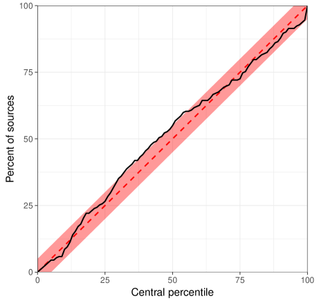
Figure 7: Percentage of sources in the primary sample whose predicted flux at epoch 2 fell within a given central percentile of a lognormal distribution with $\sigma=0.43\sqrt{2}$ centred on the flux at epoch 1. The solid line shows the data, while the dashed line shows the expected one-to-one correspondence if the model perfectly predicted the data. The shaded region encloses plus or minus five percentage points around the model prediction.

Our formalism and results are applicable for the scenario in which the redshift of the AGN is unknown. If the redshift and hence luminosity is known, then the accuracy with which the flux at a second epoch can be predicted is significantly improved. This is because the variability in X-ray luminosity of AGN is a function of luminosity, such that lower-luminosity AGN show larger fractional variability (e.g Papadakis & Lawrence, 1993; Vagnetti et al., 2016). For example, Vagnetti et al. (2016) find the fractional variability for observations separated by $\Delta t=1000$ days (rest frame) to range from $\sigma\approx 0.55$ for their least luminous AGNs ($10^{43}\mbox{$\text{~{}erg}$}\mbox{$\text{~{}s}$}^{-1}-10^{43.5}\mbox{$\text{~{}erg}$}\mbox{$\text{~{}s}$}^{-1}$ in the $0.5-4.5\mbox{$\text{~{}keV}$}$ band) down to $\sigma\approx 0.25$ for their most luminous AGNs ($10^{45}\mbox{$\text{~{}erg}$}\mbox{$\text{~{}s}$}^{-1}-10^{45.5}\mbox{$\text{~{}erg}$}\mbox{$\text{~{}s}$}^{-1}$ in the $0.5-4.5\mbox{$\text{~{}keV}$}$ band). This range in luminosity variability is naturally included in the average flux variability that we measure. However, if the redshift and hence luminosity of an AGN were known, then the results of Vagnetti et al. (2016), or similar studies, could be used to estimate a more accurate variability for that particular AGN.

5.5 Applications

This measurement of the characteristic X-ray variability of AGN has important consequences for scenarios when the flux of an AGN at one epoch must be inferred from its flux at a second. Given the uniquely high angular resolution of Chandra compared to other X-ray observatories, the most common such scenario will continue to be the use of Chandra to constrain point source contributions to observations made with other observatories.

A key example is the use of Chandra to support deep XMM-Newton observations of distant galaxy clusters, where XMM-Newton cannot resolve out the emission from projected AGN, biasing measurements of the temperature and luminosity of the cluster (e.g. Hilton et al., 2010). As demonstrated by Hilton et al. (2010), the effect of such contamination can be mitigated by jointly modelling Chandra data to constrain the AGN flux. In doing this, the uncertainty on the flux of the source due to its variability between epochs should be included. For example, if the interval between observations were a year or more, then the uncertainty on the flux prediction based on a single measurement is $\approx 60\%$. This could be modelled with a lognormal prior with $\sigma=0.6$ on the flux (or normalisation of the relevant model component) of the AGN at the epoch of the XMM-Newton observation, centred on the flux measured with Chandra. This approach will also be relevant for observations of distant clusters with ATHENA, whose angular resolution will be poorer than that of Chandra. Where possible, the interval between observations should be minimised to reduce the average variability. The same approach can be used in studies of cluster outskirts, which may optimally combine Chandra measurements of the point source population with Suzaku’s detection of the ICM (e.g. Thölken et al., 2016).

The presence of AGN can also bias the detection of galaxy clusters in X-ray surveys such as XXL (Pierre et al., 2016), XCS (Mehrtens et al., 2012) or the upcoming eROSITA survey (Pillepich et al., 2012; Merloni et al., 2012; Pillepich et al., 2018; Clerc et al., 2018). In all cases the relatively poor angular resolution of the survey data may lead to AGN being misclassified as clusters, or boost the detection probability of clusters by enhancing their surface brightness (clusters with projected AGN may also be misclassified as pure AGN and missed by these cluster surveys). The purity of such surveys can be estimated by short Chandra observations of a subset of clusters to detect the presence of contaminating AGN (Logan et. al., 2018, submitted). The variability between epochs should then be included when considering the contaminating flux (or upper limit thereon) determined from the Chandra data.

A further application of our constraints on X-ray variability is to inform the modelling of stray light in X-ray observations due to bright point sources outside the field of view. Stray light from such sources can produce faint, inhomogeneous structure in X-ray images that could bias studies of low surface brightness emission. A model of the stray light component could be produced to mitigate this, given an accurate model of the X-ray optics and knowledge of the fluxes and positions of sources outside the field of view. The latter could come from all-sky X-ray survey data. However, in the case that the stray light signal is dominated by a few bright AGN, their variability between the epoch(s) of the survey data providing their fluxes and the observation for which the stray light must be modelled will provide an irreducible limit on the precision of the stray light modelling.

6 Summary and conclusions

We have used pairs of Chandra observations of a large number of AGN to infer the characteristic X-ray variability of the population on different timescales. We developed a sample selection method that is insensitive to biases, and a likelihood model that was able to precisely recover the variability in realistic simulated data.

For our primary sample of sources observed between around 1 and 15 years apart, the variability of the population is well described by a lognormal distribution with standard deviation of $\sigma=0.43\pm 0.03$. We find evidence, in common with other work, that the variability is smaller on shorter timescales, with $\sigma\approx 0.25$ for separations of about one month to one year between observations.

Given a single flux measurement, the best estimate of the flux at a second epoch is the same as that at the first epoch (neglecting Eddington bias) with a (lognormal) $68\%$ confidence interval of $\sqrt{2}\sigma$. The factor $\sqrt{2}$ arises due to the uncertainty on the mean flux for the source given just one previous measurement.

As a rule of thumb, given the flux of an AGN at one epoch, one can estimate its flux at a second epoch (more than a year or so earlier or later) to a precision of about $60\%$.

This result has applications in a wide range of scenarios where X-ray fluxes of AGN must be inferred from their values at a different epoch, and presents a significant source of irreducible uncertainty that should be taken into account. A useful next step would be to better constrain the dependence of the variability on interval between measurements, including longer time intervals then those probed here as data become available.

Acknowledgements

BJM acknowledges support from STFC grant ST/R000700/1. THR acknowledges support by the German Aerospace Agency (DLR) with funds from the Ministry of Economy and Technology (BMWi) through grant 50 OR 1514. This project made extensive use of TOPCAT (Tool for OPerations on Catalogues And Tables Taylor, 2005). Preliminary work was done by University of Bristol undergraduate students James Battye, Jane Hesling and Nicholas Henden.

References

- Almaini et al. (2000) Almaini O., et al., 2000, MNRAS, 315, 325
- Cash (1979) Cash W., 1979, ApJ, 228, 939
- Clerc et al. (2018) Clerc N., et al., 2018, A&A, 617, A92
- Dickey & Lockman (1990) Dickey J. M., Lockman F. J., 1990, ARA&A, 28, 215
- Gehrels (1986) Gehrels N., 1986, ApJ, 303, 336
- Giles et al. (2012) Giles P. A., Maughan B. J., Birkinshaw M., Worrall D. M., Lancaster K., 2012, MNRAS, 419, 503
- Hasinger et al. (1998) Hasinger G., Burg R., Giacconi R., Schmidt M., Trumper J., Zamorani G., 1998, A&A, 329, 482
- Hilton et al. (2010) Hilton M., et al., 2010, ApJ, 718, 133
- Lawrence & Papadakis (1993) Lawrence A., Papadakis I., 1993, ApJ, 414, L85
- Lehmer et al. (2012) Lehmer B. D., et al., 2012, ApJ, 752, 46
- Mateos et al. (2007) Mateos S., Barcons X., Carrera F. J., Page M. J., Ceballos M. T., Hasinger G., Fabian A. C., 2007, A&A, 473, 105
- Mateos et al. (2008) Mateos S., et al., 2008, A&A, 492, 51
- Mehrtens et al. (2012) Mehrtens N., et al., 2012, MNRAS, 423, 1024
- Merloni et al. (2012) Merloni A., et al., 2012, astro-ph/1209.3114
- Middei et al. (2017) Middei R., Vagnetti F., Bianchi S., La Franca F., Paolillo M., Ursini F., 2017, A&A, 599, A82
- Nandra et al. (1997) Nandra K., George I. M., Mushotzky R. F., Turner T. J., Yaqoob T., 1997, ApJ, 476, 70
- Paolillo et al. (2004) Paolillo M., Schreier E. J., Giacconi R., Koekemoer A. M., Grogin N. A., 2004, ApJ, 611, 93
- Papadakis & Lawrence (1993) Papadakis I. E., Lawrence A., 1993, Nature, 361, 233
- Park et al. (2006) Park T., Kashyap V. L., Siemiginowska A., van Dyk D. A., Zezas A., Heinke C., Wargelin B. J., 2006, ApJ, 652, 610
- Pierre et al. (2016) Pierre M., et al., 2016, A&A, 592, A1
- Pillepich et al. (2012) Pillepich A., Porciani C., Reiprich T. H., 2012, MNRAS, 422, 44
- Pillepich et al. (2018) Pillepich A., Reiprich T. H., Porciani C., Borm K., Merloni A., 2018, MNRAS, 481, 613
- Somboonpanyakul et al. (2018) Somboonpanyakul T., McDonald M., Lin H. W., Stalder B., Stark A., 2018, ApJ, 863, 122
- Taylor (2005) Taylor M. B., 2005, in Shopbell P., Britton M., Ebert R., eds, Astronomical Society of the Pacific Conference Series Vol. 347, Astronomical Data Analysis Software and Systems XIV. p. 29, http://adsabs.harvard.edu/abs/2005ASPC..347...29T
- Thölken et al. (2016) Thölken S., Lovisari L., Reiprich T. H., Hasenbusch J., 2016, A&A, 592, A37
- Vagnetti et al. (2011) Vagnetti F., Turriziani S., Trevese D., 2011, A&A, 536, A84
- Vagnetti et al. (2016) Vagnetti F., Middei R., Antonucci M., Paolillo M., Serafinelli R., 2016, A&A, 593, A55