Equilibrium Formulae for Transverse Magneto-transport of Strongly Correlated Metals

Abstract

Exact formulas for the Hall coefficient [A. Auerbach, Phys. Rev. Lett. 121, 066601 (2018)], modified Nernst coefficient, and thermal Hall coefficient of metals are derived from the Kubo formula. These coefficients depend exclusively on equilibrium susceptibilities, which are significantly easier to compute than conductivities. For weak isotropic scattering, Boltzmann theory is recovered. For strong scattering, well controlled methods for thermodynamic functions are available. As an example, the Hall sign reversals of lattice bosons near the Mott insulator phases are determined. Appendices include mathematical supplements and instructions for calculating the coefficients.

I Introduction

Computation of transport coefficients of strongly correlated metals, is challenging even for minimal model Hamiltonians. DC conductivities are particularly costly, since they involve real-time correlations of large systems in the limit of long times.

The Hall coefficent $R_{H}$ – the magnetic field derivative of the transverse DC resistivity at low fields – seems to be an interesting exception. For isotropic bands, Boltzmann equation relates $R_{H}$ to the inverse carrier density. For more realistic band structures, $R_{H}$ is related to the Fermi surface curvature jones-zener ; ziman ; Ong . Thus, at least for isotropic scattering Comm-tau , $R_{H}$ is insensitive to the scattering timescale and depends only on equilibrium coefficients. (Here, “equilibrium coefficients” are defined as static derivatives of the free energy, which do not involve time dependent correlators).

$R_{H}$ raises intriguing questions: (i) Is the Hall coefficient in general an equilibrium property, beyond the validity of Boltzmann theory? (ii) Is there an explicit formula which expresses $R_{H}$ in terms of static susceptibilities? (iii) Are there other equilibrium formulas for magneto-transport coefficients of resistive metals Comm-Other ?

These questions are particularly relevant to “bad metals”, where scattering rates exceed the Fermi energy badmetals ; lindner and quasiparticles are not well-defined. Bad metals are known to exhibit “Hall anomalies” – poorly understood magnetic field, temperature, and doping dependences of the Hall coefficient, including unexpected sign reversals. Hall anomalies have been observed in strongly disordered films smith ; kapitulnik , resistive phases of unconventional superconductors hagen ; Taillefer , strongly correlated metallic paramagnets Lior , and more. Resolving the origin of the Hall anomalies has been hampered by the innaplicability of Boltzmann equation, and the formidable numerical challenges of DC conductivities.

In a recent paper Assa-PRL , Questions (i) and (ii), have been answered by the derivation of a formula for $R_{H}$, which depends solely on equilibrium susceptibilities. The formula is applicable to general interacting and disordered Hamiltonians. The coefficients are amenable to well controlled numerical algorithms including: high temperature series domb , variational wavefunctions DMRG , Quantum Monte Carlo simulations prokofiev ; assaad (in imaginary time), and more. Most importantly, the Hall coefficient does not depend on real-time DC conductivities, which inherently involve less controlled and much costlier computations Comm-RT ; White ; MaxEnt ; snir-QMC .

This paper reviews and expands the derivation of the Hall coefficient formula Assa-PRL . It also answers Question (iii) by deriving two additional equilibrium formulas for transverse magneto-transport coefficients. It opens up the possibility for feasibly computing magnetotransport coefficients for strongly correlated Hamiltonians.

Three formulas are presented in this paper:

1. The Hall coefficient is

   $$R_{H}\equiv\sigma_{xx}^{-2}~{}{d\sigma_{H}\over dB}\Big{|}_{B\!=\!0},$$ (1)

   where $\sigma_{H}$ and $\sigma_{xx}$ are the Hall and longitudinal conductivities respectively, and $B$ is the perpendicular magnetic field. The formula is

   $$R_{H} = R_{H}^{(0)}+R_{H}^{\rm corr},$$

   $$R_{H}^{(0)} = -{\mbox{Im}}{\left(j^{x}|[M,j^{y}]\right)-\left(j^{y}|[M,j^{x}]\right)\over\hbar{\cal V}\mu_{0}^{2}},$$ (2)

   where $M$ is the total magnetization operator, $j^{\alpha},~{}\alpha=x,y$ are the uniform $({\bf q}\!=\!0$) electric currents, and ${\cal V}$ is the system’s volume in $d$ dimensions. $(A|B)$ is a static mutual susceptibility of operators $A$ and $B$,

   $$(A|B)\equiv-\partial_{h_{A}}\partial_{h_{B}}{\mbox{Tr}}\log e^{-(\beta H-h_{A}A-h_{B}B)}\Big{|}_{h_{A},h_{B}\!=\!0},$$ (3)

   where $H$ is the zero field Hamiltonian. $\mu_{0}=(j^{\alpha}|j^{\alpha})/{\cal V}$, is the zeroth moment of the conductivity (f-sum rule). The correction $R_{H}^{\rm corr}$ is defined by Eq. (LABEL:HallN) in Section III.

2. The modified Nernst coefficient is

   $$W={1\over\sigma_{xx}\kappa_{xx}}{d\alpha_{xy}\over dB}\Big{|}_{B\!=\!0},$$ (4)

   where $\kappa_{xx}$ is the thermal conductivity, and $\alpha_{xy}$ is the transverse thermoelectric (TTE) coefficient behnia-review . The formula is

   $$W \equiv W^{(0)}+W^{\rm corr},$$

   $$W^{(0)} \equiv {1\over\hbar\mu_{0}^{Q}\mu_{0}}\left((j_{Q}^{x}|[M,j^{y}])-(j_{Q}^{y}|[M,j^{x}])\right),$$ (5)

   where $j_{Q}^{\alpha},\alpha=x,y$ are the thermal currents, and $\mu_{Q}=(j_{Q}^{\alpha}|j_{Q}^{\alpha})/{\cal V}$ is the thermal sum rule shastry-sumrules . The correction $W^{\rm corr}$ is defined in Eq. (LABEL:nu-star1) in Section IV.

3. The thermal Hall coefficient is

   $$R_{TH}={1\over\kappa_{xx}^{2}}{d\kappa_{xy}\over dB}\Bigg{|}_{B\!=\!0},$$ (6)

   where $\kappa_{xy}$ is the thermal Hall conductivity. The formula is

   $$R_{TH} = R_{TH}^{(0)}+R_{TH}^{\rm corr},$$

   $$R_{TH}^{(0)} \equiv {T\over\hbar{\cal V}(\mu_{0}^{Q})^{2}}\left(\left(j_{Q}^{x}|[M,j_{Q}^{y}]\right)\!-\!\left(j_{Q}^{y}|[M,j^{y}_{Q}]\right)\right).$$ (7)

   The correction $R_{TH}^{\rm corr}$ is defined in Eq. (LABEL:R-TH1) in Section V.

The correction terms $R_{H}^{\rm corr}$, $W^{\rm corr}$, and $R_{TH}^{\rm corr}$ are sums over rational functions of equilibrium susceptibilities of local operators. These operators are constructed by multiple commutators of $M$, $H$ and the uniform electrical and thermal currents.

Here we are interested in strongly correlated metals which are not amenable to perturbative expansions or to Boltzmann’s transport theory. The derivation of Eqs. (2), (5) and (7) starts with the many-body Kubo formula in the Lehmann (eigenstate) representation. Numerical evaluation of this representation requires exponentially large memory cost. Bogoliubov operator hyperspace and Krylov operators formulation Bogoliubov ; MerminWagner ; Mori provide a very useful framework for our derivations.

The reader may not be a-priori familiar with hyperspace terminology, which will be fully defined in the following sections. We note that hyperspace has been extensively used to generate memory functions for transport theory forster ; zwanzig ; wolfle .

Bogoliubov hyperspace provides essential advantages:

• Avoids the prohibitive cost of exact diagonalization required for the Lehmann representation of the Kubo formula.

• Charts a direct route to continued fraction expansions of conductivities of strongly correlated metals MHLee ; viswanath ; Sandvik ; lindner ; khait ,

• Enables a convenient framework for differentiating the conductivities with respect to magnetic field.

The latter advantage is a key ingredient in the proofs given below.

Application of our formulas to models of electrons and bosons is instructive. The zeroth terms $R^{(0)}_{H}$, $W^{(0)}$, and $R^{(0)}_{TH}$ recover Boltzmann equation result in the constant lifetime approximation. Anisotropic lifetime effects appear in higher order corrections. For lattice bosons, we locate the Hall sign changes in the vicinity of the Mott insulator lobes. From these examples we learn that low energy renormalization of the microscopic Hamiltonian can greatly enhance the relative magnitudes of the zeroth terms relative to the harder-to-compute correction terms.

This paper is organized as follows. Section II introduces the Kubo formulas for the Hall and TTE conductivities in Bogoliubov hyperspace notations. Section III derives the Hall coefficient formula, Eq. (LABEL:HallN). Section IV derives the modified Nernst coefficient formula, Eq. (LABEL:nu-star1). Section V derives the thermal Hall coefficient formula, Eq. (LABEL:R-TH1).

Section VI discusses applications of the formulas to effective Hamiltonians, band electrons, and strongly interacting lattice bosons.

Section VII is peripherally connected to the bulk of this paper. From the Kubo formula, some known relations between equilibrium observables and conductivities are derived: The Streda formulas Streda ; McD , Chern numbers TKNN ; yosi ; huber , and Hall-pumped polarization Chern-pump-theory ; prelov-ladder ; Chern-pump-exp . The derivation clarifies why these relations are restricted to bulk-incompressible, non-dissipative systems where $\sigma_{xx}\!=\!0$.

The paper is concluded by a summary and proposals for applications of our formulas to interesting models.

The appendices contain instructive technical details for computing the formulas. Appendix A constructs Krylov bases in the Bogoliubov hyperspace. Appendix B expands the longitudinal conductivities $\sigma_{xx}(\omega)and\kappa_{xx}(\omega)$ as continued fractions. Appendix C explains how to compute the moments, recurrents and magnetization matrix elements as equilibrium coefficients. Appendix D describes the variational extrapolation of recurrents scheme, which obtains dynamical response functions from a finite set of moments. Appendix E calculates the Liouvillian Green function and shows how the DC conductivities factor out of the magneto-transport coefficients. This is the key result which proves that the coefficients are purely equilibrium quantities.

II Kubo formula in hypespace notations

DC conductivities of metals are defined (using an infinitesimal ${\varepsilon}$ prescription) by the following order of limits

$$\sigma_{\alpha\beta}\equiv\lim_{\omega\to 0}\lim_{{\bf q}\to 0}\lim_{{\varepsilon}\to 0}\lim_{{\cal V}\to\infty}\sigma_{\alpha\beta}({\bf q},\omega;{\cal V},{\varepsilon}),$$ (8)

where the dynamical conductivities are given by the Kubo formula

$$\sigma_{\alpha\beta}({\bf q},\omega) = {\hbar\over{\cal V}}{\mbox{Im}}\sum_{n,m}{(\rho_{n}\!-\!\rho_{m})\langle m|j^{\alpha}_{{\bf q}}|n\rangle\langle n|j^{\beta}_{-{\bf q}}|m\rangle\over(E_{m}\!-\!E_{n})(E_{m}\!-\!E_{n}-\hbar\omega\!-\!i{\varepsilon})},$$ (9)

$$= {\hbar\over{\cal V}}{\mbox{Im}}\left(j_{{\bf q}}^{\alpha}\Big{|}\left({1\over{\cal L}-\hbar\omega-i{\varepsilon}}\right)\Big{|}j_{{\bf q}}^{\beta}\right).$$

$j^{\alpha}_{\bf q}$ are the spatial Fourier components of currents, and $\alpha$ denotes both the transported quantity (charge or heat) and the direction of the current $x$ or $y$. $E_{n}$ and $|n\rangle$ are the eigenenergies and eigenstates of the grand Hamiltonian, $H-\mu N$, respectively. $\rho_{n}=e^{-\beta E_{n}}/{\mbox{Tr}}e^{-\beta(H-\mu N)}$ are Boltzmann weights. Henceforth, we avoid the “$\lim$” symbols for the DC limit, remembering the order of limits in (8).

For pedagogical simplicity, we restrict ourselves to a uniform magnetic field ${\bf B}=B\hat{{\bf z}}$. For $B=0$, all response functions (after disorder averaging) obey C4m symmetry (reflections and rotations around $\hat{{\bf z}}$). Hence $\sigma_{xx}=\sigma_{yy}$ and $\sigma_{xy}=-\sigma_{yx}\equiv\sigma_{H}$.

The DC limit of a metal requires large system sizes, since ${\cal V}^{-1/d}\leq\omega/v\to 0$ for some finite velocity scale $v$. Memory requirements blow up as $e^{{\cal V}}$, which is prohibitively costly, even for minimal Hamiltonians of strongly correlated metals, such as the Hubbard, t-J, and Kondo lattice models. Hyperspace formulation, in the second line of Eq. (9), avoids the eigenstate representation.

Hyperspace notations: The set of operators $\{A\}$ in Schroedinger Hilbert space define hypestates $|A)$ with the inner product Mori

$$(A|B)\equiv\sum_{nm}{\rho_{n}-\rho_{m}\over E_{m}-E_{n}}\langle m|A^{\dagger}|n\rangle\langle n|B|m\rangle$$ (10)

$(A|B)$ depends on temperature and is physically an equilibrium susceptibility given by Eq. (3). It can also be written as an imaginary-time correlation function, see Eq. (114). We denote a normalized hyperstate by an angular bracket $|A\rangle$.

The Liouvillian ${\cal L}$ is a hermitian hyperoperator that acts on hyperstate $|A)$ by ${\cal L}|A)=\big{|}[H,A]\big{)}$. The DC hyper-resolvent can be separated into

$$\left({1\over{\cal L}-i{\varepsilon}}\right)\equiv\left({1\over{\cal L}}\right)^{\prime}+i\left({1\over{\cal L}}\right)^{\prime\prime}$$ (11)

where

$$\left({1\over{\cal L}}\right)^{\prime} = {{\cal L}\over{\cal L}^{2}+{\varepsilon}^{2}},$$

$$\left({1\over{\cal L}}\right)^{\prime\prime} = {{\varepsilon}\over{\cal L}^{2}+{\varepsilon}^{2}}.$$ (12)

We shall find it useful to write the inner product, Eq. (10), as a trace in Schroedinger space

$$(A|B)=-{\mbox{Tr}}\rho\left[\left({1\over{\cal L}}\right)^{\prime}A^{\dagger},B\right].$$ (13)

By Eq. (9), the Hall conductivity is given by the off-diagonal matrix element in hyperspace

$$\sigma_{H}={\hbar\over{\cal V}}{\mbox{Im}}\left(j^{x}\Big{|}\left({1\over{\cal L}}\right)^{\prime}\Big{|}j^{y}\right).$$ (14)

C4m and time reversal symmetries ensure that $\sigma_{H}$ is antisymmetric in $x{\rightarrow\atop\leftarrow}y$, and in $B\to-B$.

Similarly, the antisymmetrized TTE coefficient is given by

$$\alpha_{xy}={\hbar\over T{\cal V}}{\cal A}_{xy}{\mbox{Im}}\left(j_{Q}^{x}\Big{|}\left({1\over{\cal L}}\right)^{\prime}\Big{|}j^{y}\right)-{c\over T{\cal V}}\langle M^{\rm orb}\rangle,$$

(15)

where $j_{Q}^{\alpha}$ is the thermal current in the $\alpha$ direction, and ${\cal A}_{xy}$ is the antisymmetrizer defined by ${\cal A}_{xy}f(x,y)={1\over 2}(f(x,y)-f(y,x))$.

The orbital magnetization in the $\hat{{\bf z}}$ direction is

$$M^{\rm orb}={q\over 2c}\sum_{i=1}^{N}{\bf x}_{i}\times{\bf v}_{i}\cdot\hat{{\bf z}},$$ (16)

which must be included in Eq. (15) in order to satisfy Onsager’s time reversal relations Cooper . $N$ is the number of particles with charge $q$, positions ${\bf x}_{i}$ and velocities ${\bf v}_{i}$.

Finally, the thermal Hall conductivity is given by Cooper

$$\kappa_{xy} = {\hbar\over T{\cal V}}{\cal A}_{xy}{\mbox{Im}}\left(j_{Q}^{x}\Big{|}\left({1\over{\cal L}}\right)^{\prime}\Big{|}j_{Q}^{y}\right)$$ (17)

$$~{}~{}~{}~{}-{2\over T{\cal V}}\langle M^{Q}\rangle,$$

where

$$M^{Q}={1\over 4}\sum_{i=1}^{N}{\bf x}_{i}\times\{{\bf v}_{i},h_{i}-\mu\}\cdot\hat{{\bf z}}$$ (18)

is the thermal magnetization.

In Appendix B, the continued fractions of longitudinal conductivities $\sigma_{xx}$ and $\kappa_{xx}$ are derived, and the algorithm to compute their recurrents is reviewed. However, transverse coefficients $\sigma_{H}$, $\alpha_{xy}$, and $\kappa_{xy}$ are off-diagonal matrix elements of the hyper-resolvent and, therefore, are not readily expressed as computable continued fractions.

III Derivation of the Hall coefficient formula

While Eq. (1) is a ratio of transverse and longitudinal Kubo formulas [see Eq. (9)], we find that the expression simplifies considerably by taking the derivative of $\sigma_{H}$ with respect to magnetic field Comm-derivation . We thus assume differentiability of the transport coefficients at zero field in the paramagnetic, dissipative phase:

$$\sigma_{xx}(B)=\sigma_{xx}+{\cal O}(B^{2}),~{}~{}~{}\sigma_{H}\propto B+{\cal O}(B^{3}).$$ (19)

The conditions in Eq. (19) preclude zero resistivity and quantum Hall phases, which are amenable to the equilibrium relations of Section VII.

Using Eq. (13), the Hall conductivity in Eq. (14) is written as

$$\sigma_{H}=-{\hbar\over{\cal V}}{\mbox{Im}}{\mbox{Tr}}\rho\left[\left({1\over{\cal L}}\right)^{\prime}j^{x},\left({1\over{\cal L}}\right)^{\prime}j^{y}\right].$$ (20)

In non-periodic Euclidean space, one can define two commuting polarization operators:

$$P^{\alpha}=q\sum_{i=1}^{N}x^{\alpha}_{i},~{}~{}~{}\alpha=x,y.$$ (21)

The uniform electric currents are given by the operators

$$j^{\alpha}={i\over\hbar}~{}{\cal L}P^{\alpha}.$$ (22)

Using Eq. (12) in Eq. (22), we obtain

$$\left({1\over{\cal L}}\right)^{\prime}j^{\alpha} = {i\over\hbar}\left({{\cal L}\over{\cal L}^{2}+{\varepsilon}^{2}}\right){\cal L}P^{\alpha},$$ (23)

$$= {i\over\hbar}\left(P^{\alpha}-{\tilde{P}}^{\alpha}\right),$$

where ${\tilde{P}}^{\alpha}$ is the projection of $P^{\alpha}$ onto the ${\varepsilon}$-broadened kernel of ${\cal L}$,

$${\tilde{P}}^{\alpha}\equiv\left({{\varepsilon}^{2}\over{\cal L}^{2}+{\varepsilon}^{2}}\right)P^{\alpha}.$$ (24)

In Fig. 1, the operators $P^{x}-{\tilde{P}}^{x}$ and ${\tilde{P}}^{x}$ are depicted as submatrices of $P^{x}$ in the Lehmann representation.

Two points should be noted about $P^{\alpha}$: (i) For systems with periodic boundary conditions in $\alpha$-direction (e.g. on a sphere, torus, cylinder, or ring), $P^{\alpha}and{\tilde{P}}^{\alpha}$ cannot be defined. For such cases, alternate expressions for $\left({1\over{\cal L}}\right)^{\prime}j^{\alpha}$ are given in Section VII. (ii) For translationally invariant Hamiltonians (no spatially varying potentials), $q^{-1}{\tilde{P}}^{\alpha}=R^{\alpha}$ are the global guiding center symmetries of $H$. Their algebra, $[R^{x},R^{y}]=-i{\hbar c\over eB}$, gives rise to an extensive Landau-level degeneracy. In dissipative metals, which concern this paper, $R^{\alpha}$ are not symmetries, and Landau level degeneracy is lifted by potentials and interactions.

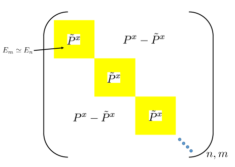
Figure 1: The projection operator $P^{x}$ represented in the eigenenergy basis of $H$. The projected polarization ${\tilde{P}}^{x}$ in the degenerate subspaces is marked by yellow blocks, and $P^{x}-{\tilde{P}}^{x}$ is supported in the white areas.

Finally, the Hall conductivity in Euclidean space can be written as

$$\sigma_{H}={1\over\hbar{\cal V}}{\mbox{Im}}{\mbox{Tr}}\rho\left[P^{x}-{\tilde{P}}^{x},P^{y}-{\tilde{P}}^{y}\right],$$ (25)

where, by Eq. (8), we send ${\varepsilon}\to 0$ after ${\cal V}\to\infty$ to obtain the equilibrium conductivity. The “bare” electric polarizations in Eq. (21) are independent of $B$ and mutually commute: $[P^{x},P^{y}]=0$. However, the contributions of ${\tilde{P}}^{\alpha}$ to the commutator in Eq. (25) survive in the presence of a finite magnetic field, even as the limit ${\varepsilon}\to 0$ is taken, leading to $\sigma_{H}\neq 0$. This is shown by the expressions derived below.

Taking the derivative of Eq. (25) with respect to magnetic field yields two terms

$${d\sigma_{H}\over dB}\Bigg{|}_{B\!=\!0} = \Xi_{\rho}+\Xi_{\cal M},$$

$$\Xi_{\rho} = -{q^{2}\over\hbar{\cal V}}{\mbox{Im}}{\mbox{Tr}}{d\rho\over dB}\left[P^{x}-{\tilde{P}}^{x},P^{y}-{\tilde{P}}^{y}\right]_{B\!=\!0},$$

$$\Xi_{\cal M} = -{q^{2}\over\hbar{\cal V}}{\mbox{Im}}{\mbox{Tr}}\rho\left[-{d{\tilde{P}}^{x}\over dB},P^{y}-{\tilde{P}}^{y}\right]_{B\!=\!0}$$ (26)

$$-{q^{2}\over\hbar{\cal V}}{\mbox{Im}}{\mbox{Tr}}\rho\left[P^{x}-{\tilde{P}}^{x},-{d{\tilde{P}}^{y}\over dB}\right]_{B\!=\!0}.$$

$\Xi_{\rho}$ is evaluated using the operator identity

$${d\rho\over dB}=\beta\rho(M_{d}-\langle M\rangle)-\left[\rho,\left({1\over{\cal L}}\right)^{\prime}M\right],$$ (27)

where $M=-{\partial H\over\partial B}$ is the magnetization, and $M_{d}$ is its energy-diagonal part $[H,M_{d}]=0$. Thus,

$$\lim_{B\to 0}\Xi_{\rho} = {\beta\over\hbar{\cal V}}{\mbox{Im}}\beta\left(M\Big{|}\left[P^{x}\!-\!{\tilde{P}}^{x},P^{y}\!-\!{\tilde{P}}^{y}\right]\right)$$ (28)

$$~{}~{}+{1\over\hbar{\cal V}}{\mbox{Im}}{\mbox{Tr}}\rho(M_{d}\!-\!\langle M\rangle)\left[P^{x}\!-\!{\tilde{P}}^{x},P^{y}\!-\!{\tilde{P}}^{y}\right]$$

$$= 0.$$

Both terms of $\Xi_{\rho}$ vanish at zero magnetic field by time reversal symmetry.

To evaluate $\Xi_{\cal M}$, the derivative ${d{\tilde{P}}^{\alpha}\over dB}$ uses the hyperoperator identity

$${d\over dB}\left({1\over{\cal O}(B)}\right)=-{1\over{\cal O}}{d{\cal O}\over dB}{1\over{\cal O}},$$ (29)

where ${\cal O}={\varepsilon}^{2}/({\cal L}^{2}(B)+{\varepsilon}^{2})$. This yields

$${d{\tilde{P}}^{\alpha}\over dB}=-{{\varepsilon}\over{\cal L}^{2}+{\varepsilon}^{2}}({\cal M}{\cal L}+{\cal L}{\cal M}){{\varepsilon}\over{\cal L}^{2}+{\varepsilon}^{2}}P^{\alpha},$$

$$~{}~{}=-i\hbar\left({1\over{\cal L}}\right)^{\prime\prime}{\cal M}\left({1\over{\cal L}}\right)^{\prime\prime}j^{\alpha}+{\cal L}\left({1\over{\cal L}}\right)^{\prime\prime}{\cal M}\left({1\over{\cal L}}\right)^{\prime\prime}P^{\alpha},$$

(30)

where ${\cal M}=-{\partial{\cal L}\over\partial B}\equiv[M,\bullet]$ is the hypermagnetization.

Thus, casting $\Xi_{\cal M}$ as an inner product using Eq. (13), and using the hermiticity of ${\cal L}$, yields

$${d\sigma_{H}\over dB}\Bigg{|}_{B\!=\!0}=-{2\hbar\over{\cal V}}{\cal A}_{xy}{\mbox{Im}}\left(j^{x}\Big{|}\left({1\over{\cal L}}\right)^{\prime\prime}{\cal M}\left({1\over{\cal L}}\right)^{\prime\prime}\Big{|}j^{y}\right)+\Xi^{\prime}.$$ (31)

The second term vanishes

$$\Xi^{\prime}=-{\hbar\over{\cal V}}{\cal A}_{xy}{\mbox{Im}}\left({\cal L}j^{x}\Big{|}\left({1\over{\cal L}}\right)^{\prime\prime}{\cal M}\left({1\over{\cal L}}\right)^{\prime\prime}\Big{|}P^{y}\right)=0,$$ (32)

due to the hermiticity of ${\cal L}$ and the identity proven in Appendix E,

$$\left({1\over{\cal L}}\right)^{\prime\prime}~{}{\cal L}~{}j^{\alpha}=0~{}.$$ (33)

Now we simplify Eq. (31) by inserting resolutions of identities between the hyperoperators. For that purpose, we introduce the Krylov basis of orthonormal operators $\{|n/_{j^{\alpha}}\rangle\}$, which are constructed by sequentially applying ${\cal L}$ to the root state, the current $|j^{\alpha})$, and orthonormalizing. Details are provided in Appendix A. We note that $\langle n/_{j^{x}}|m/_{j^{y}}\rangle=0$ due to the C4m symmetry at zero magnetic field.

The Krylov bases provide partial resolutions of identity [see Eq. (120)]:

$$\sum_{n=0}^{\infty}|n/_{j^{\alpha}}\rangle\langle|n/_{j^{\alpha}}|=1_{{\cal S}_{j^{\alpha}}},~{}~{}~{}\alpha=x,y,$$ (34)

where ${\cal S}_{j^{\alpha}}$ is the subspace spanned by $\{{\cal L}^{n}|j^{\alpha})\}_{n=0}^{\infty}$.

Application of Eq. (34) on the respective sides of ${\cal M}$ in Eq. (31) yields a double sum

$${d\sigma_{H}\over dB}\Bigg{|}_{B\!=\!0}=-{2\hbar\mu_{0}}{\cal A}_{xy}\sum_{m,n=0}^{\infty}\langle 0/_{j^{x}}\Big{|}\left({1\over{\cal L}}\right)^{\prime\prime}\Big{|}m/_{j^{x}}\rangle$$

$$~{}~{}~{}~{}\times{\mbox{Im}}\langle m/_{j^{x}}|{\cal M}|n/_{j^{y}}\rangle\langle n/_{j^{y}}\Big{|}\left({1\over{\cal L}}\right)^{\prime\prime}\Big{|}0/_{j^{y}}\rangle,$$

$$={\hbar\mu_{0}}\sum_{m,n=0}^{\infty}G^{\prime\prime}_{0,m}G^{\prime\prime}_{n,0}M^{\prime\prime}_{m,n},$$

$$M^{\prime\prime}_{m,n}\equiv{\mbox{Im}}\left(\langle m/_{j^{x}}|{\cal M}|n/_{j^{y}}\rangle-\langle m/_{j^{y}}|{\cal M}|n/_{j^{x}}\rangle\right).$$ (35)

The imaginary hyperresolvent matrix lements $G^{\prime\prime}_{0,n}=G^{\prime\prime}_{n,0}$ are evaluated in Appendix E [see Eq. (141)]:

$$G^{\prime\prime}_{n,0} = \langle n/_{j^{y}}\Big{|}\left({1\over{\cal L}}\right)^{\prime\prime}\Big{|}0/_{j^{y}}\rangle\times\delta_{n,{\rm even}},$$

$$G^{\prime\prime}_{2k,0}(0) = -\sigma_{xx}~{}{R_{k}\over\hbar\mu_{0}},$$

$$R_{k} = \prod_{j=1}^{k}\left(-{\Delta_{2j-1}\over\Delta_{2j}}\right),$$ (36)

which shows that the longitudinal conductivity $\sigma^{2}_{xx}$ factors out of the double sum in Eq. (35). Using the definition of the Hall coefficient in Eq. (1), $\sigma_{xx}^{2}$ cancels out from $R_{H}$. This is a key result of the derivation!

The final formula for the Hall coefficient is thus

$$R_{H} = R_{H}^{(0)}+R_{H}^{\rm corr},$$

$$R_{H}^{(0)} \equiv -{\mbox{Im}}{\left(j^{x}|{\cal M}|j^{y}\right)-\left(j^{y}|{\cal M}|j^{x}\right)\over{\cal V}\hbar\mu_{0}^{2}},$$

$$R_{H}^{\rm corr} \equiv -{1\over\hbar\mu_{0}}\sum_{i,k=0}^{\infty}(1-\delta_{i,0}\delta_{k,0})R_{i}R_{k}M^{\prime\prime}_{2i,2k}.$$

Eq. (LABEL:HallN) defines $R_{H}^{\rm corr}$, which was presented earlier in Eq. (2). $R_{k}$, defined by Eq. (36), depends on a finite set of conductivity recurrents $\Delta_{i},i\leq 2k$, as defined in Appendix B. A recipe for their computation is given in Appendix C. The hypermagnetization matrix elements $M^{\prime\prime}_{2i,2k}$ require computing mutual susceptibilities of operators, such as $\Big{|}2i/_{j^{x}}\Big{\rangle}$ and $\Big{|}\left[M,|2k/_{j^{y}}\rangle\right]\Big{)}$.

In a non-critical, paramagnetic metal, $R_{H}<\infty$. Therefore, the double sum $\sum_{i,k}$ in $R_{H}^{\rm corr}$ is expected to (conditionally) converge, and its terms to decrease as $i,k\to\infty$. The rate of convergence depends on the particular Hamiltonian, but it could be estimated by computing a finite sequence of terms.

As shown in Section VI, the relative magnitudes $R_{H}^{\rm corr}/R_{H}^{(0)}$ could be greatly decreased at low temperatures by renormalizing the microscopic Hamiltonian onto an effective Hamiltonian.

IV The modified Nernst coefficient

In this section and the next (Section V), the derivations follow similar steps as in the previous section. Hence the discussion is briefer. To define the thermal current we need to be more specific about the Hamiltonian $H$. We consider $N$ particles (either bosons or fermions) of charge $q$ described by a general continuum Hamiltonian

$$H = \sum_{i=1}^{N}h_{i},$$

$$h_{i} \equiv h_{1}\left({\bf p}_{i},{\bf x}_{i},{\bf S}_{i};B\right)+{1\over 2}\sum_{j,j\neq i}U_{ij}~{}.$$ (38)

Here, the single particle Hamiltonian $h_{1}$ includes kinetic, potential, and spin energies. $U_{ij}$ is a short range, two-body interaction.

In close analogy to the electric polarizations $P^{\alpha}$, we define the thermal polarizations

$$Q^{\alpha}={1\over 2}\sum_{i=1}^{N}\{x^{\alpha}_{i},h_{i}-\mu\},~{}~{}~{}\alpha=x,y.$$ (39)

The heat current is simply the time derivative of the thermal polarization

$$j^{\alpha}_{Q}({\bf q}\!=\!0)\equiv{i\over\hbar}{\cal L}Q^{x}\simeq{1\over 2}\sum_{i=1}^{N}\{v^{\alpha}_{i},h_{i}-\mu\}.$$ (40)

Henceforth we neglect, for notational simplicity, the nonlocal contributions to $j^{\alpha}_{Q}$ of the form $({\bf v}_{i}+{\bf v}_{j})\cdot\nabla U_{ij}(x^{\alpha}_{i}-x_{j}^{\alpha})$ Hardy . These can be included, but they contribute minor effects for short range interactions $U_{ij}$.

Following the analogous derivation which led to Eq. (25), we use Eqs. (13) and (40) to express Eq. (15) as

$$\alpha_{xy}={q\over\hbar T{\cal V}}{\cal A}_{xy}{\mbox{Im}}{\mbox{Tr}}\rho\left[Q^{x}-{\tilde{Q}}^{x},P^{y}-{\tilde{P}}^{y}\right]-{c\over T{\cal V}}\langle M^{\rm orb}\rangle,$$ (41)

where

$${\tilde{Q}}^{x}\equiv\left({{\varepsilon}^{2}\over{\cal L}^{2}+{\varepsilon}^{2}}\right)Q^{x}.$$ (42)

The commutator between thermal and electric polarizations is nonzero:

$${\cal A}_{xy}[Q^{x},P^{y}]={i\hbar\over 2}\sum_{i}(x_{i}v^{y}_{i}-y_{i}v^{x}_{i})=i{\hbar c\over q}M^{\rm orb},$$ (43)

which precisely cancels against the orbital magnetization term in Eq. (41), leaving us with

$$\alpha_{xy}={q\over\hbar TV}{\cal A}_{xy}{\mbox{Im}}{\mbox{Tr}}\rho\left[-{\tilde{Q}}^{x},P^{y}-{\tilde{P}}^{y}\right]+\left[Q^{x}-{\tilde{Q}}^{x},-{\tilde{P}}^{y}\right].$$ (44)

Differentiating Eq. (44) with respect to $B$ at $B=0$ yields the following terms

$${d\alpha_{xy}\over dB}\Bigg{|}_{B\!=\!0}=-{\hbar\over TV}{\cal A}_{xy}{\mbox{Im}}{\mbox{Tr}}\rho\left[-{d{\tilde{Q}}^{x}\over dB},P^{y}\right]+\left[P^{x},-{d{\tilde{Q}}^{y}\over dB}\right],$$ (45)

where we discard, as in Eq. (28), time reversal symmetry breaking terms from ${d\rho\over dB}$, as well as the (undifferentiated) ${\tilde{P}},{\tilde{Q}}$ operators, which contribute corrections of ${\cal O}({\varepsilon})$.

$d{\tilde{Q}}^{x}/dB$ yields two terms

$${d{\tilde{Q}}^{\alpha}\over dB} = -i\hbar\left({1\over{\cal L}}\right)^{\prime\prime}{\cal M}\left({1\over{\cal L}}\right)^{\prime\prime}j_{Q}^{\alpha}$$ (46)

$$-{{\varepsilon}^{2}\over{\cal L}^{2}+{\varepsilon}^{2}}\sum_{i=1}^{N}x^{\alpha}_{i}m_{i},$$

where the second term contributes ${\cal O}({\varepsilon})$ to Eq. (45) and can be discarded.

Following the analogous derivation of Eq. (31) leads to

$${d\alpha_{xy}\over dB}=-{2\hbar\over T{\cal V}}$$

$$~{}~{}~{}\times{\cal A}_{xy}{\mbox{Im}}\left(j_{Q}^{x}\Big{|}\left({1\over{\cal L}}\right)^{\prime\prime}{\cal M}\left({1\over{\cal L}}\right)^{\prime\prime}\Big{|}j^{y}\right).$$ (47)

The Krylov thermal resolution of identity is

$$\sum_{n=0}^{\infty}|n/_{j_{Q}^{\alpha}}\rangle\langle n/_{j_{Q}^{\alpha}}|=1_{{\cal S}_{j_{Q}^{\alpha}}}.$$ (48)

Inserting the thermal resolution of identity from Eq. (48) on the left of ${\cal M}$ in Eq. (47) and the electric resolution of identity from Eq. (34) on its right results in

$${d\alpha_{xy}\over dB}\Big{|}_{B\!=\!0} = -{\sigma_{xx}\kappa_{xx}\over\hbar(\mu_{0}^{Q}\mu_{0})^{1\over 2}}$$

$$\times\sum_{i,k}R^{Q}_{i}R_{k}{M^{Q}_{2i,2k}}^{\prime\prime},$$

$${M^{Q}_{2i,2k}}^{\prime\prime} \equiv {\mbox{Im}}\left(\langle 2i/_{j_{Q}^{x}}|{\cal M}|2k/_{j^{y}}\rangle-\langle 2i/_{j_{Q}^{y}}|{\cal M}|2k/_{j^{x}}\rangle\right),$$

where $\mu_{Q}={1\over{\cal V}}(j_{Q}^{x}|j_{Q}^{x})$ is the thermal conductivity sum rule shastry-sumrules .

The factors

$$R^{Q}_{i}=\prod_{j=1}^{i}\left(-{\Delta^{Q}_{2j-1}\over\Delta^{Q}_{2j}}\right),$$ (50)

depend on the recurrents $\Delta^{Q}_{n}$ of the thermal conductivity $\kappa_{xx}$, as defined in Eq. (132).

The modified Nernst coefficient defined by Eq. (4) is given by the formula

$$W = {1\over\sigma_{xx}\kappa_{xx}}{d\alpha_{xy}\over dB}\Big{|}_{B\!=\!0},$$

$$= W^{(0)}+W^{\rm corr},$$

$$W^{(0)} \equiv {1\over\hbar\mu_{0}^{Q}\mu_{0}}\left((j_{Q}^{x}|{\cal M}|j^{y})-(j_{Q}^{y}{\cal M}|j^{x})\right),$$

$$W^{\rm corr} \equiv {1\over\hbar(\mu_{0}^{Q}\mu_{0})^{1\over 2}}\sum_{i,k}R^{Q}_{i}R_{k}{M^{Q}_{2i,2k}}^{\prime\prime}(1-\delta_{i,0}\delta_{k,0}).$$

This equation defines $W^{\rm corr}$, which was presented in Eq. (5).

$W$ is related to the Nernst coefficient $\nu$ as follows:

$$\nu = {d\over dB}\left({E_{x}\over-{dT\over dy}}\right)_{B\!=\!0},$$

$$= \left(\sigma_{xx}^{-1}{d\alpha_{xy}\over dB}-R_{H}\alpha_{xx}\right)_{B\!=\!0},$$

$$W = {\nu+R_{H}\alpha_{xx}\over\kappa_{xx}}.$$ (52)

For special particle-hole symmetric systems, $R_{H},\alpha_{xx}=0$, and the relation simplifies to $W=\nu/\kappa_{xx}$.

V The Thermal Hall Coefficient

The thermal Hall coefficient is the derivative of the thermal Hall resistivity with respect to magnetic field at zero field. The thermal Hall conductivity in Eq. (17) is given in Euclidean geometry by

$$\kappa_{xy}={1\over\hbar T{\cal V}}{\cal A}_{xy}{\mbox{Im}}{\mbox{Tr}}\rho\left[Q^{x}-{\tilde{Q}}^{x},Q^{y}-{\tilde{Q}}^{y}\right]-{2\over T{\cal V}}\langle M^{Q}\rangle,$$ (53)

where the thermal magnetization correction $M^{Q}$ is defined by Eq. (18).

The antisymmetrized commutator between “bare” thermal polarizations yields

$${\cal A}_{xy}[Q^{x},Q^{y}] = {i\hbar\over 2}\sum_{i}\left(x_{i}\{v^{y}_{i},h_{i}-\mu\}-y_{i}\{v^{x}_{i},h_{i}-\mu\}\right),$$ (54)

$$= i{2\hbar}M^{Q},$$

which precisely cancels against the second term in Eq. (53), leaving us with

$$\kappa_{xy}={1\over\hbar TV}{\cal A}_{xy}{\mbox{Im}}{\mbox{Tr}}\rho\left[-{\tilde{Q}}^{x},Q^{y}-{\tilde{Q}}^{y}\right]+\left[Q^{x}-{\tilde{Q}}^{x},-{\tilde{Q}}^{y}\right].$$ (55)

Differentiating ${\tilde{Q}}^{\alpha}$ with respect to $B$, and discarding all terms of order ${\varepsilon}$ yields

$${d\kappa_{xy}\over dB}=-{2\hbar\over T{\cal V}}$$

$$~{}~{}~{}\times{\cal A}_{xy}{\mbox{Im}}\left(j_{Q}^{x}\Big{|}\left({1\over{\cal L}}\right)^{\prime\prime}{\cal M}\left({1\over{\cal L}}\right)^{\prime\prime}\Big{|}j_{Q}^{y}\right).$$ (56)

Now we insert two thermal resolutions of identities from Eq. (48) and divide out $\kappa_{xx}^{2}$, as defined by Eq. (6), to obtain

$$R_{TH} = R_{TH}^{(0)}+R_{TH}^{\rm corr},$$

$$R_{TH}^{(0)} \equiv {T\over\hbar(\mu_{0}^{Q})^{2}}\left(\left(j_{Q}^{x}|{\cal M}|j_{Q}^{y}\right)-\left(j_{Q}^{y}|{\cal M}|j^{x}_{Q}\right)\right),$$

$$R_{TH}^{\rm corr} \equiv {T\over\hbar\mu_{0}^{Q}}\sum_{i,k}R^{Q}_{i}R^{Q}_{k}{M^{QQ}_{2i,2k}}^{\prime\prime}(1-\delta_{i,0}\delta_{k,0}),$$

$${M^{QQ}_{2i,2k}}^{\prime\prime} \equiv {\mbox{Im}}\left(\langle 2i/_{j_{Q}^{x}}|{\cal M}|2k/_{j_{Q}^{y}}\rangle-\langle 2i/_{j_{Q}^{y}}|{\cal M}|2k/_{j_{Q}^{x}}\rangle\right).$$

The factors $R^{Q}_{n}$ are defined in Eq. (50). This equation defines $R_{TH}^{\rm corr}$, which was presented in Eq. (7).

VI Applications to Effective Models

It is greatly advantageous at low temperatures to replace the microscopic Hamiltonian $H({\bf A})$, where ${\bf A}$ is the electromagnetic vector potential, by an effective Hamiltonian $\bar{H}({\bf A})$ for two reasons:

1. Reduction of the Hilbert space size, which greatly facilitates numerical computations.

2. Rearrangement of the sums in Eqs. (LABEL:HallN) and (LABEL:nu-star1) by increasing the relative size of $R_{H}^{(0)}$ relative to $R_{H}^{\rm corr}$.

Eqs. (31), (47), and (56) show that the two coefficients, at low temperatures, are determined solely by the low energy part of Hilbert space. Let us examine Eq. (31) in the Lehmann representation

$${d\sigma_{H}\over dB}\Bigg{|}_{B\!=\!0}=-{2\pi^{2}\hbar\over{\cal V}}{\cal A}_{xy}\sum_{nmk}{\rho_{m}\!-\!\rho_{n}\over E_{n}\!-\!E_{m}}j^{x}_{nm}\delta(E_{m}\!-\!E_{n})$$

$$~{}~{}\times\left(M_{mk}j^{y}_{kn}\delta(E_{k}\!-\!E_{n})-j^{y}_{mk}M_{kn}\delta(E_{m}\!-\!E_{k})\right)).$$ (58)

The energy conserving $\delta$ functions ensure that all participating states in the sum are (up to order ${\varepsilon}$) degenerate $E_{n}\simeq E_{m}\simeq E_{k}$ and restricted by Boltzmann weights to energies less than some cut-off $\Lambda>k_{B}T$. We can therefore substitute $H\to\bar{H}$, which shares the same low energy spectrum in a reduced Hilbert space, i.e.

$$\bar{E}_{n}=E_{n},~{}~{}~{}E_{n}\leq\Lambda.$$ (59)

All currents and magnetization in Eq. (31) should also be replaced by their renormalized counterparts given by

$$j^{\alpha}\to\bar{j}^{\alpha} = -c{\partial\bar{H}\over\partial A^{\alpha}},$$

$$M\to\bar{M} = -{\partial\bar{H}\over\partial B}.$$ (60)

Each individual term in the summation formulas is altered by the renormalization, since the Krylov bases, recurrents, and hypermagnetization matrix elements all depend on the renormalized operators. However, an exact renormalization must leave Eq. (31) identical to that of the microscopic Hamiltonian.

In many practical circumstances, approximate renormalization are implemented. These include Schrieffer-Wolff transformations SW , Brillouin-Wigner perturbation theory IEQM , and Contractor Renormalization (CORE) CORE-marvin ; CORE-altman ; p6 .

As a demonstration of the advantages of effective Hamiltonians, we compute $R_{H}^{(0)}$ for a microscopic Hamiltonian

$$H=\sum_{i=1}^{N}{({\bf p}-{q\over c}{\bf A})^{2}\over 2m}+V({\bf x}_{i})+{1\over 2}\sum_{i\neq j}U({\bf x}_{i}-{\bf x}_{j})+V^{\rm dis},$$ (61)

where $V$ is a periodic lattice potential, and $V^{\rm dis}$ describes a disorder potential. The microscopic currents and magnetization obey

$$j^{\alpha} = q\sum_{i}{{\bf p}^{\alpha}\over m},$$

$$M = {q\over 2mc}\sum_{i}{\bf x}_{i}\times{\bf p}_{i},$$

$$\left[M,j^{\alpha}\right] = {iq\hbar\over 2mc}\sum_{\beta}\epsilon_{\alpha\beta}j^{\beta},$$

$${\mbox{Im}}(j^{\alpha}|{\cal M}|j^{\beta}) = {\hbar V\over 2c}\mu_{0}\epsilon_{\alpha\beta},$$

$$\mu_{0} = {1\over\hbar{\cal V}}{\mbox{Im}}\langle\left[P^{x},q\sum_{i}{p^{x}_{i}\over m}\right]\rangle,$$ (62)

$$= {Nq^{2}\over{\cal V}m},$$

where $\epsilon_{\alpha\beta}$ is the antisymmetric tensor.

By Eq. (62), the zeroth Hall coefficient term is inversely proportional to the total density

$$R^{(0)}_{H}={{\cal V}\over Nqc}.$$ (63)

VI.1 A single conduction band

If the chemical potential lies within a single band, separated by a large interband gap from other bands, it is possible to describe the low spectrum by an effective single band model

$$\bar{H}=\sum_{{\bf k}s}(\epsilon_{ks}-\mu)c^{\dagger}_{{\bf k}s}c_{{\bf k}s}+\sum_{{\bf k}s}\bar{V}^{\rm dis}_{{\bf k}{\bf k}^{\prime}}c^{\dagger}_{{\bf k},s}c_{{\bf k}^{\prime}s},$$ (64)

where $c^{\dagger}_{{\bf k},s}$ creates a band electron of charge $e$ and spin $s$ at lattice wavevector ${\bf k}$. $\epsilon_{\bf k}$ is the band dispersion, and $\bar{V}^{\rm dis}$ is the intraband disorder potential.

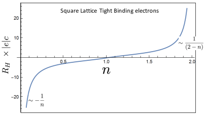
Figure 2: Hall coefficient versus electron filling, at low temperature, for the weakly disordered square lattice tight binding model, as given by Eq. (66).

The single-band currents and magnetization are

$$\bar{j}^{\alpha} = e\sum_{ks}v^{\alpha}_{{\bf k}s}c^{\dagger}_{{\bf k}s}c_{{\bf k}s},$$

$$\bar{M} = {ie\hbar\over 2c}\sum_{ks}c^{\dagger}_{{\bf k}s}\left(v^{y}_{{\bf k}s}{d\over dk^{x}}-v^{x}_{{\bf k}s}{d\over dk^{y}}\right)c_{{\bf k}s},$$ (65)

where $v_{\bf k}^{\alpha}={\partial\epsilon_{\bf k}\over\partial k^{\alpha}}$. Hence

$$\bar{R}_{H}^{(0)} = -{1\over{\cal V}}{{\mbox{Im}}\left(\left(\bar{j}^{x}|\bar{{\cal M}}|\bar{j}^{y}\right)-\left(\bar{j}^{y}|\bar{{\cal M}}|\bar{j}^{x}\right)\right)\over\hbar\mu_{0}^{2}},$$ (66)

$$= 2{e^{3}\over c\mu_{0}^{2}}\int{d^{d}k\over(2\pi)^{d}}\left(-{\partial f\over\partial\epsilon}\right)F_{\bf k},$$

where the mean Fermi surface curvature is given by

$$F_{\bf k}=(v^{x}_{\bf k})^{2}{\partial^{2}\epsilon_{\bf k}\over(\partial k^{y})^{2}}+(v^{y}_{\bf k})^{2}{\partial^{2}\epsilon_{\bf k}\over(\partial k^{x})^{2}}-2v^{x}_{\bf k}v^{y}_{\bf k}{\partial^{2}\epsilon_{\bf k}\over\partial k^{y}\partial k^{x}},$$ (67)

and the zeroth moment (f-sum rule) is

$$\mu_{0}=2e^{2}\int{d^{d}k\over(2\pi)^{d}}\left(-{\partial f\over\partial\epsilon}\right)|v^{x}_{\bf k}|^{2}.$$ (68)

Eq. (66) recovers Boltzmann equation result jones-zener ; ziman in the case of wavevector-independent scattering time. In Fig. 2, Eq.(66) for the square lattice tight model is plotted as a function of electron filling.

A single parabolic bandstructure

$$\epsilon_{\bf k}=-\mbox{\rm sign}(e){\hbar^{2}|{\bf k}|^{2}\over 2m^{*}},$$ (69)

where $e<0$ ($e>0$) describes electrons (holes) respectively, yields $\mu_{0}={ne^{2}\over m^{*}}$. Its Hall coefficient is equal to the famous Drude result

$$\bar{R}_{H}^{(0)}={1\over nec},$$ (70)

where $ne$ is the charge density of this single band.

The corrections $\bar{R}_{H}^{\rm corr}$ depend only on the weak impurity scattering $\bar{V}^{\rm dis}$, since

$$\bar{{\cal L}}j^{y}=e\sum_{{\bf k},{\bf k}^{\prime}}\bar{V}^{\rm dis}_{{\bf k},{\bf k}^{\prime}}(v^{x}_{\bf k}-v^{x}_{{\bf k}^{\prime}})c^{\dagger}_{{\bf k}s}c_{{\bf k}^{\prime}s}.$$ (71)

Thus the factor $\Delta_{1}/\Delta_{2}$ which enters the coefficients $R_{k},k\geq 1$, is suppressed as ${\cal O}(\sqrt{\langle(\bar{V}^{\rm dis})^{2}\rangle}/\epsilon_{F}\ll 1$ at weak disorder, where $\epsilon_{F}$ is the Fermi energy.

Recall that the $R_{H}^{(0)}$ of Eq. (63) was inversely proportional to the total density $N/{\cal V}$, including all core and valence electrons. For the effective single band model, the corrections were found to be suppressed at weak disorder, $\bar{R}_{H}^{\rm corr}/\bar{R}_{H}^{(0)}\ll 1$. Therefore, for the original microscopic Hamiltonian, $R_{H}^{\rm corr}$ is relatively large and could even reverse the sign of $R_{H}^{(0)}$. The lesson learned is that renormalization of $H$ onto the single band model allows one to fully include the single body periodic potential into the renormalized zeroth term of the Hall coefficient and, therefore, greatly reduce the magnitude of the correction term.

Comment on lifetime anisotropy: The Hall coefficient for the case of a ${\bf k}$-dependent lifetime $\tau_{\bf k}$ is given by Boltzmann equation jones-zener ; ziman ; Ong as

$$R_{H}^{\rm Boltz} = 2{e^{3}\over c(\sigma^{\rm Boltz}_{xx})^{2}}\int{d^{d}k\over(2\pi)^{d}}\left(-{\partial f\over\partial\epsilon}\right)F_{\bf k}\tau_{\bf k}^{2},$$

$$\sigma^{\rm Boltz}_{xx} = 2e^{2}\int{d^{d}k\over(2\pi)^{d}}\left(-{\partial f\over\partial\epsilon}\right)|v^{x}_{\bf k}|^{2}\tau_{\bf k}.$$ (72)

The anisotropy factor $(\tau^{2}_{\bf k}-\langle\tau\rangle^{2})/\langle\tau\rangle^{2}$ on the Fermi surface is a consequence of anisotropic scattering by impurities, phonons, and other electrons. These effects are missing in $\bar{R}_{H}^{(0)}$ of Eq. (66), which depends only on the band structure. Application of the fully interacting Liouvillian when constructing the higher order Krylov states introduces the anisotropies of the scattering operators, of the type shown in Eq. (71). However, at low temperatures and for weak scattering potentials, Eq. (71) is simpler than computing $R_{H}^{\rm corr}$. Nevertheless, Eq. (LABEL:HallN) teaches us that lifetime anisotropy effects can be described by equilibrium susceptibilities.

The modified Nermst coefficient of a single band Hamiltonian in Eq. (64) is

$$W^{(0)} = {2e\over c\mu_{0}\mu^{Q}_{0}}\int{d^{d}k\over(2\pi)^{d}}\left(-{\partial f\over\partial\epsilon}\right)(\epsilon_{\bf k}-\mu)F_{\bf k},$$

$$\mu^{Q}_{0} = 2\int{d^{d}k\over(2\pi)^{d}}\left(-{\partial f\over\partial\epsilon}\right)(\epsilon_{\bf k}-\mu)|v^{x}_{\bf k}|^{2},$$ (73)

$$= {\pi^{2}\over 3}{k_{B}^{2}\over e^{2}}T^{2}\mu_{0}+{\cal O}(T^{3}),$$

where, for the last line, we used a low temperature Sommerfeld expansion behnia-book .

Similarly, the thermal Hall coefficient is given by

$$R_{TH}^{(0)} = 2{eT\over c(\mu_{Q})^{2}}\int{d^{d}k\over(2\pi)^{d}}\left(-{\partial f\over\partial\epsilon}\right)(\epsilon_{\bf k}-\mu)^{2}F_{\bf k}.$$

Application of these results to the parabolic band model from Eq. (69) yields the simple expressions

$$W^{(0)} = {1\over n\epsilon_{F}c},$$

$$R_{TH}^{(0)} = {3e\over\pi^{2}k_{B}}~{}{1\over nTc}.$$ (75)

For parabolic bands, the inverse of $W$ ($R_{TH}$) measures the number density times the Fermi energy (temperature).

VI.2 Hard Core Bosons (HCB)

Repulsively interacting bosons in a deep periodic potential with square lattice symmetry are described by,

$$H=\sum_{i}\left({({\bf p}_{i}-{q\over c}{\bf A})^{2}\over 2m}+V({\bf x}_{i})\right)+{1\over 2}\sum_{i\neq j}U(|{\bf x}_{i}-{\bf x}_{j}|).$$ (76)

This model may be renormalized onto a single-band, Bose-Hubbard model BHM-Fisher (using $\hbar=c=1$)

$$\bar{H}=-t\sum_{\langle ij\rangle}e^{-iqA_{ij}}a^{\dagger}_{i}a_{j}+{\rm h.c.}+U\sum_{i}n_{i}^{2},$$ (77)

where $a_{i}^{\dagger}$ creates a boson on site $i$, and $A_{ij}=\int_{{\bf x}_{i}}^{{\bf x}_{j}}d{\bf x}\cdot{\bf A}$. At strong interactions, when the average filling is between two integers $j<\langle n_{i}\rangle<j+1$, the fluid phase is “squeezed” between two insulating phases. The effective Hamiltonian for that regime is well described by further renormalization onto the Hard Core Bosons (HCB) model lindner

$$\bar{H}^{\rm HCB}=-t\sum_{\langle ij\rangle}e^{-iqA_{ij}}S^{+}_{i}S^{-}_{j}+\mbox{h.c.},$$ (78)

where $\bf{S}$ are pseudospin half operators. $S_{i}^{+}$ creates a HCB at site $i$, and $S_{i}^{z}\!=\!n_{i}-{1\over 2}$ measures its fluctuations in its occupation numbers. The Hall coefficient vanishes at $\langle n\rangle={1\over 2}$ by emergent particle hole symmetry, which can be verified by $S^{+}\to S^{-}$ and $S^{z}\to-S^{z}$ in Eq. (78). The renormalized currents and magnetizations are

$$\bar{j}^{\alpha} = -iqt\sum_{i}\left(e^{-iqA_{ii+\alpha}}S^{+}_{i}S^{-}_{i+\alpha}-\mbox{h.c.}\right),$$

$$\bar{M} = {q\over 2}\sum_{i}x_{i}\bar{j}^{y}_{i+y}-y_{i}\bar{j}^{x}_{i,i+x}.$$ (79)

Expanding Eq.(3) in powers of $\beta$ at high temperatures yields

$$(A|B)=\beta{\mbox{Tr}}\rho_{\infty}A^{\dagger}B-{\beta^{2}\over 2}{\mbox{Tr}}\rho_{\infty}\{H,A^{\dagger}\}B+{\cal O}(\beta^{3}).$$ (80)

The infinite temperature density matrix $\rho_{\infty}$ projects onto a fixed particle number

$$\sum_{i}{\mbox{Tr}}\left(\rho_{\infty}S^{z}_{i}\right)=(n-{1\over 2})V.$$ (81)

Thus

$$\mu_{0}\!=\!\beta{\mbox{Tr}}\rho_{\infty}j_{i,i+x}^{2}.$$ (82)

One can verify that all magnetization matrix elements $M_{2j,2k}^{\prime\prime}$ vanish unless the operators in the trace encircle a magnetic flux. Therefore, for a triangular lattice at high temperatures SSS , $M_{0,0}^{\prime\prime}\!\propto\!-\beta(n-{1\over 2})$, while for a square lattice, $M^{\prime\prime}_{0,0}\!\propto\!-\beta^{2}(n-{1\over 2})$. Thus we obtain for the triangular and square lattices

$$\bar{R}_{H}^{(0)}\propto\left\{\begin{array}[]{ll}-T(n-{1\over 2})&\mbox{triangular}\\ -(n-{1\over 2})&\mbox{square}\\ \end{array}\right.~{}.$$ (83)

Correction terms that involve $\bar{M}_{2j,2k}^{\prime\prime}$ decay rapidly with $j,k$ due to diminishing overlaps between Krylov states. Thus the Hall sign changes around half filling lines are denoted by HCB in Fig. 3.

VI.3 Quantum Rotors (QR)

For the same Bose-Hubbard model in Eq. (77) near the Mott phases at integer filling $n_{0}$, the fluid state can be described by the Quantum Rotors (QR) field theory

$$\bar{H}^{\rm QR}=\int d^{d}x{1\over 2\chi_{c}}(\rho({\bf x})-n_{0}a^{-d})^{2}+{1\over 2}\rho_{s}\left(\nabla\varphi({\bf x})+{q\over c}{\bf A}\right)^{2}(1+\gamma\rho({\bf x})^{2})+V({\bf x})\rho({\bf x}),$$ (84)

where $a$ is the lattice constant, $\chi_{c}$ is the local compressibility, and $\rho_{s}$ is the local superfluid stiffness. $\rho$ is the deviation of the density from the commensurate filling $n_{0}$ of the neighboring Mott phase. The QR theory can be derived from a quantum Josephson junction array model, where $\chi_{c}$ are the grain capacitances, and $\rho_{s}$ are intergrain Josephson couplings.

From the phase diagram of the Bose-Hubbard model, it is clear that $\gamma>0$, since the superfluid stiffness and ground state order parameter are enhanced as the density is varied away from $n_{0}$.

The canonical density-phase commutations are Com3

$$[\rho({\bf x}),\varphi({\bf x}^{\prime})]=-i\delta({\bf x}-{\bf x}^{\prime}).$$ (85)

The QR currents and magnetization densities are

$$\bar{{\bf j}}({\bf x}) = -q\rho_{s}\nabla\varphi(1+\gamma\rho^{2}),$$

$$\bar{m}({\bf x}) = -{q\over 2c}\left(xj^{y}({\bf x})-yj^{x}({\bf x})\right).$$ (86)

Notice that the factors $\gamma\rho^{2}$ are necessary to produce current dynamics via nonvanishing commutators ${\cal M}j^{\alpha}$ and ${\cal L}j^{\alpha}$. There is no Hall effect at the particle-hole symmetric line $\langle\rho\rangle=0$.

Using Eq. (85), the sign of the Hall coefficient can be obtained

$$R_{H}^{(0)}\propto{\gamma\over q\rho_{s}c}\langle\rho\rangle+{\cal O}(\langle\rho^{3}\rangle),$$ (87)

which implies a particle-like Hall effect above the commensurate filling, and a hole-like effect below. As for the band electrons, higher order corrections of $R_{H}^{\rm corr}$ are negligible at weak disorder.

In Fig. 3 we combine the results of HCB and QR models to map the Hall signs of the Bose-Hubbard model in the nonsuperfluid (metallic) phase. While the Hall conductivity of metallic phases are not simply related to Chern numbers on finite tori (see Section VII), it is interesting that our results in Fig. 3 are consistent with the Hall signs as evaluated by Huber and Lindner huber .

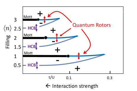
Figure 3: Hall signs in strong interactions regime of the Bose-Hubbard model Eq. (77). Mott insulators are thick black lines, ending at critical points (black circles). Solid blue lines mark Hall sign changes at zero temperature, computed by Huber and Lindnerhuber . At high temperatures, we find the same sign changes using Hard Core Bosons (HCB) and Quantum Rotors, in Eqs. (83) and (87,) respectively.

VII Streda formulas, Chern Numbers and Hall-pumped Polarization

This section is peripheral to the bulk of the paper and is included for completeness of our discussion of equilibrium magneto-transport coefficients. We derive some previously known relations for Hall and TTE conductivities, which are applicable to nondissipative phases and high magnetic fields.

VII.1 Translationally invariant systems

The Hall coefficient of a perfectly translationally invariant system Girvin ; Cooper subject to a uniform electric field ${\bf E}=E^{y}\hat{{\bf y}}$ is readily solved by a Galilean transformation to a moving frame of velocity

$$v^{x}=c{E_{y}\over B},$$ (88)

where the electric field is transformed to zero in the moving frame. Absence of moving potentials implies that the current vanishes in the moving frame. Hence, back in the lab frame the current is

$$\langle j^{x}\rangle=qn{\bf v}=\sigma_{H}E^{y}~{}~{}\leadsto~{}\sigma^{\rm hom}_{H}={nqc\over B},$$ (89)

where $nq$ is the charge density, and

$$\langle j^{x}_{Q}\rangle=T{S\over N}nv^{x}=T\alpha_{xy}E^{y}~{}~{}\leadsto~{}\alpha^{\rm hom}_{xy}={s\over B},$$ (90)

where $s=S/{\cal V}$ is the entropy density behnia-review . Eqs. (89) and (90) apply at any density, magnetic field and two-body interactions, as long as there are no spatially varying potentials, and consequenty zero resistivity.

VII.2 Streda formulas for $\sigma_{H}$ and $\alpha_{xy}$

An equilibrium formula for the Hall conductivity was proposed by Streda Streda

$$\tilde{\sigma}_{H}=c\left({\partial\rho\over\partial B}\right)_{\mu,T}=c\left({\partial m\over\partial\mu}\right)_{\rho,T},$$ (91)

where $\rho$ and $m$ are the charge and magnetization density respectively.

For the TTE, a similar Streda formula is

$$\tilde{\alpha}_{xy}=c\left({\partial s\over\partial B}\right)_{\mu,T}.$$ (92)

Here we show that both Streda formulas are related to the static long wavelength conductivities. Note that these imply the reverse order of limits than the DC limit in Eq (8). That is to say,

$$\tilde{\sigma}_{H} = \lim_{{\bf q}\to 0}\sigma_{H}({\bf q},0)$$

$$\tilde{\alpha}_{xy} = \lim_{{\bf q}\to 0}\alpha_{xy}({\bf q},0).$$ (93)

Proof: The continuity equation relates charge density $\rho$ to current density

$$\dot{\rho}({\bf x})={i\over\hbar}{\cal L}\rho=-\nabla\cdot{\bf j}({\bf x}).$$ (94)

By a Fourier transformation

$${1\over\hbar}{\cal L}\rho_{\bf q}=-{\bf q}\cdot{\bf j}_{\bf q},$$ (95)

the relation between magnetization (in the $z$ direction) and magnetization currents ${\bf j}_{m}$ is

$$\nabla\times{\bf M}={1\over c}{\bf j}_{m}.$$ (96)

Without loss of generality, we choose ${\bf q}=(q_{x},0)$, ${\bf j}_{m}=(0,j^{y})$, and ${\bf M}_{\bf q}=M_{\bf q}\hat{{\bf z}}$. Thus we can write

$$j^{x}_{\bf q} = -{1\over\hbar q_{x}}{\cal L}\rho_{\bf q}$$

$$\to\left({1\over{\cal L}}\right)^{\prime}j_{\bf q}^{x} = -{1\over\hbar q_{x}}\rho_{\bf q},$$ (97)

and

$$j^{y}_{\bf q}=icq_{x}M_{\bf q}.$$ (98)

Using Eqs. (9), (97), (98), we obtain

$$\lim_{{\bf q}\to 0}\sigma_{H}({\bf q},0) = \lim_{{\bf q}\to 0}\lim_{{\cal V}\to\infty}{1\over{\cal V}}{\mbox{Re}}\Big{(}\rho_{\bf q}\Big{|}M_{{\bf q}}\Big{)},$$ (99)

$$= c\left({\partial\rho\over\partial B}\right)_{\mu,T}.$$

Similarly, using a Fourier transform of Eq. (40) for the TTE coefficient yields

$$j_{Q}^{x}({\bf q})={1\over\hbar q_{x}}{\cal L}(h_{\bf q}-\mu n_{\bf q}).$$ (100)

Rewriting Eq. (15) using Eqs. (98) and (100) yields

$$\lim_{\omega\to 0}\alpha_{xy}({\bf q},\omega)={c\over T{\cal V}}\left(\left(h_{\bf q}-\mu n_{\bf q}\Big{|}M_{\bf q}\right)-\langle M_{\bf q}\rangle\right).$$ (101)

Taking the limit ${\bf q}\to 0$ of Eq. (101) and using the equilibrium relation

$$\left({d(E-\mu N-TS)\over dB}\right)_{\mu,T}=\langle M\rangle,$$ (102)

where $S$ is the entropy, we obtain

$$\tilde{\alpha}_{xy}\equiv\lim_{{\bf q}\to 0}\lim_{{\cal V}\to\infty}\alpha_{xy}({\bf q},0)=c\left({\partial s\over\partial B}\right)_{\mu,T},$$ (103)

where $s={S\over{\cal V}}$ is the entropy density, which completes the proof of Eq. (93). Q.E.D.

Eq. (93) allows us to investigate sufficient conditions for permitting reversal of order-of-limits, required by Eq. (8). If there exists an equilibrium gap $E_{\rm gap}=\lim_{{\bf q}\!=\!0}{\rm min}_{n}(E_{n}({\bf q})-E_{0})\gg T>0$ which survives the limit of ${\cal V}\to\infty$, surely the order of limits can be reversed. This is permitted in quantum Hall phases, where the only gapless regions are at the sample edges Comm-Streda . On the other hand, metals at weak magnetic fields are gapless in the bulk, and not described by the Streda formulas.

VII.3 Chern numbers on the torus

A finite gauged torus is penetrated by a uniform magnetic field with integer total flux $N_{\Phi}\Phi_{0}$. Here, $\Phi_{0}=hc/q$, where $q$ is the charge of the particles. Its two holes are threaded by Aharonov-Bohm fluxes ${\theta_{\alpha}\over 2\pi}\Phi_{0},\alpha=x,y$.

Aharonov-Bohm (AB) fluxes can be introduced by adding source terms to the Hamiltonian

$$H\to H-{\hbar\over q}\left(j^{x}\theta_{x}/L_{x}+j^{y}\theta_{y}/L_{y}\right).$$ (104)

On the torus, we cannot define polarization operators. Nevertheless, we can relate write the matrix elements of $\left({1\over{\cal L}}\right)^{\prime}j^{\alpha}$ using first-order perturbation theory in $\theta_{y}$ to eigenstate $|n\rangle$, as

$$\langle m|\left({1\over{\cal L}}\right)^{\prime}j^{\alpha}|n\rangle = {\langle m|j^{x}|n\rangle\over E_{m}-E_{n}},$$ (105)

$$= {L_{x}q\over\hbar}\Big{\langle}m|{\partial\over\partial\theta_{x}}n\Big{\rangle}_{\vec{\theta}=0}.$$

Substituting Eq. (105) into Eq. (20), the Hall conductance of the torus is

$$\Sigma_{H}(L_{x},L_{y})=2{q^{2}\over\hbar}\sum_{n=0}^{\infty}\rho_{n}{\mbox{Im}}\Big{\langle}{\partial\over\partial\theta_{y}}\psi_{n}\Big{|}{\partial\over\partial\theta_{x}}\psi_{n}\Big{\rangle}_{\vec{\theta}=0},$$ (106)

which is the thermally averaged Chern curvature at zero AB fluxes.

Avron and Seiler yosi , using adiabatic transport theory, related the ground state Hall conductance to the integral of the Chern curvature over the AB fluxes (the reciprocal torus):

$$\Sigma^{\rm Chern}_{H} = \int_{0}^{2\pi}\int_{0}^{2\pi}{d\theta_{x}d\theta_{y}\over(2\pi)^{2}}~{}\Sigma_{H}(\theta_{x},\theta_{y},T\!=\!0),$$ (107)

$$= {q^{2}\over h}\int_{0}^{2\pi}\int_{0}^{2\pi}{d\theta_{x}d\theta_{y}\over\pi}~{}{\mbox{Im}}\Big{\langle}{\partial\over\partial\theta_{y}}\psi_{0}\Big{|}{\partial\over\partial\theta_{x}}\psi_{0}\Big{\rangle},$$

$$= {q^{2}\over h}\times\mbox{\rm Integer}.$$

The double integral over a smooth Chern curvature yields a topological integer called Chern number TKNN ; yosi . In the limit of large tori with a finite gap, the Chern curvature at weak magnetic field is expected to approach its average, and the two expressions in Eqs. (106) and (107) coincide.

The important conclusion from relating the Chern number to $\Sigma_{H}$ is that the Hall conductance is quantized as long as the conditions of adiabatic transport theory hold. Eq. (106) is a static equilibrium calculation. At low temperatures, it requires only the knowledge of the lowest eigenstates lindnerHall .

Huber and Lindner (HL) huber proved an important theorem about ground state Chern numbers of charged particles in periodic potentials.
HL Theorem: Consider $N$ particles (fermions or bosons) of charge $q$ on the surface of a torus, in a periodic potential of $N_{\rm sites}$ unit cells, and a perpendicular uniform magnetic field of comensurate flux $N_{\phi}\Phi_{0}$, where $N_{\rm sites}/N_{\phi}$ is integer.

$$\Sigma^{\rm Chern}_{H}={q^{2}\over h}\left(\nu+m{N_{\rm sites}\over N_{\phi}}\right),$$ (108)

where $\nu={N\over N_{\phi}}$ is the filling factor, and $m$ is any integer.

Proof: Define a flux quantum cell of size $(L^{\Phi_{0}}_{x},L^{\Phi_{0}}_{y})$, such that $L^{\Phi_{0}}_{x}\times L^{\Phi_{0}}_{y}=N_{\rm sites}/N_{\phi}$. Because of the relation between translations of the null lines of the vector potential in $H$ lindnerHall and changes in the AB fluxes, the Chern curvatures (which are gauge invariant) are periodic in the AB fluxes with the corresponding periodicity $\Delta\theta_{x}=2\pi/L^{\Phi_{0}}_{x}$, $\Delta\theta_{y}=2\pi/L^{\Phi_{0}}_{y}$ respectively. Any change in the Chern number can occur by a level crossing, which can introduce an integer change in the total Chern number $m=\pm 1,\pm 2\ldots$.

We first consider a free Hamiltonian with zero potential energy. Galilean symmetry requires

$$\Sigma^{\rm Free}_{H}={nqc\over B}={q^{2}\over h}\nu.$$ (109)

By the argument above, turning on the periodic potential adiabatically can only change the Chern number by an integer $m$ multiplied by the number of periodic flux quanta unit cells $N/N_{\phi}$, which results in Eq. (108). QED.

A change with $m=-1$ reverses the Hall sign, which is expected above half filling for HCB lindnerHall . For noninteracting tight binding electrons on a bipartite lattice berg , $m=-2$ across the half filling boundary.

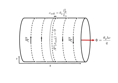
Figure 4: The gauged cylinder. A finite cylinder penetrated by a radial magnetic field, and Aharonov-Bohm flux $\Phi$. $L_{y}$ is the circumference, and $l_{B}=\sqrt{\hbar c\over qB}$ is the magnetic length. $A^{y}$ is the vector potential, whose null line at $x_{\rm null}$ moves as a function of $\theta_{y}$, whilst pumping the charge polarization.

VII.4 Hall-pumped polarization on the cylinder

Hall conductance on a finite cylinder is related to the Hall-pumped polarization Chern-pump-theory ; prelov-ladder . We assume periodicity of $H$ in the $y$-direction and open boundary conditions on the $x$ axis (see Fig. 4). For charge $q$ particles, $x$-polarization is

$$P^{x}=q\sum_{i}x_{i}.$$ (110)

A small AB flux $\theta_{y}\hbar c/q$ is introduced through the cylinder’s hole by adding to the Hamiltonian

$$H\to H-{\hbar\over qL_{y}}j^{y}\theta_{y}.$$ (111)

Inserting Eqs. (20) and (23) into Eq. (105), the cylinder’s Hall conductance is given by

$$\Sigma^{\rm pump}_{H} = {q\over\hbar L_{x}}\sum_{n=0}^{\infty}\rho_{n}$$ (112)

$$~{}\times\left(\langle\psi_{n}|P^{x}|{d\over d\theta_{y}}\psi_{n}\rangle+\langle{d\over d\theta_{y}}\psi_{n}|P^{x}|\psi_{n}\rangle\right),$$

$$= {q\over\hbar L_{x}}\sum_{n=0}^{\infty}\rho_{n}{dP^{x}(n,\theta_{y})\over d\theta_{y}}\Big{|}_{\theta_{y}=0},$$

$$= {q\over\hbar L_{x}}{d\over d\theta_{y}}\langle P^{x}\rangle\Big{|}_{\theta_{y}=0}.$$

This result can be interpreted as adiabatic pumping of the polarization, as depicted in Fig. 4. By reflection symmetry, we can define $\langle P^{x}\rangle=0$ for $\theta_{y}=0$. The “null line” at $x=x_{\rm null}$ lindnerHall is defined by vanishing Wilson loop $\oint dyA_{y}(x_{\rm null})=0$. Adiabatically increasing $\theta_{y}\to\Delta\theta_{y}$ moves the null line an incremental distance

$$\Delta x_{\rm null}=\Delta\theta_{y}{L^{x}\over 2\pi N_{\phi}}$$ (113)

along the $x$ axis. If there are non level crossings, the variation of Hamiltonian and its eigenstates adiabatically pumps the polarization. If the pumping takes time $\tau$, the $x$-current is given by $I_{x}={1\over L_{x}}\Delta\langle P^{x}\rangle/\tau$, and the $y$-voltage is $V^{y}={\hbar\Delta\theta_{y}\over q\tau}$, which yields Eq. (112) for $\Sigma^{\rm pump}_{H}=I_{x}/V_{y}$.

$P^{x}(\theta_{y})$ is a thermodynamic average which can be computed at any fixed $\theta_{y}$ by equilibrium approaches. For example, using a variational matrix product state as provided by e.g. Density Matrix Renormalization group DMRG .

Caveat: The relevance of Chern curvatures and numbers and Hall-pumped polarization to the limit ${\cal V}\to\infty$ depends on an absence of level crossings for infinitesimal changes of AB fluxes $\Delta\theta$. These can give rise to dissipative relaxation of the polarization. The incompressible quantum Hall phases satisfy this condition. Their polarization can only relax by charge tunneling between far away edge excitations whose rate is suppressed exponentially in the distance between edges, for both integer and fractional quantum Hall phases Assa-QH . However, adaibatic transport fails for bulk-gapless disordered metals, where nonadiabatic (Zener tunneling) at arbitrary weak electric field gives rise to a dissipative conductivity $\sigma_{xx}>0$.

VIII Summary and Discussion

The main purpose of this paper was to derive formulas for the Hall, modified Nernst, and thermal Hall coefficients, which avoid computing DC conductivities. Quite remarkably, these coefficients for dissipative metals of $\sigma_{xx}>0$ depend on the free energy and its static derivatives. As such, they are now amenable to a variety of well-developed numerical methods, which could be applied to interesting models of strongly interacting electrons and bosons, such as the Hubbard and t-J models IEQM ; Ilia for cuprates and metals near Mott insulators, the Kondo latice model for heavy fermions hewson , Weyl semimetals ari-weyl , cold atoms on optical lattices with an artificial magnetic field Chern-pump-exp , and more.

The zeroth terms $R_{H}^{(0)}$, $W^{(0)}$, and $R_{TH}^{(0)}$ are relatively simple and can be evaluated analytically in certain models and limits (e.g. weak interactions, or lattice models at high temperature). The correction terms require susceptibilities of more complicated operators. Since the sums are expected to converge for noncritical metals, the higher order terms should decrease in magnitude, but the rate depends on the model and temperature regime. In practice, the first few terms could provide an estimate of the convergence rate and the truncation error.

As our examples show in Section VI, large potential variations and two body interactions may be renormalized at low energies into simpler effective Hamiltonians. The single band model for weakly interacting electrons and hard core bosons and quantum rotors for strongly interacting bosons are such examples. By renormalization, qualitative features of magneto-transport coefficients, such as sign changes, temperature, and doping dependences, may be extracted already from the zeroth order coefficients.

Strong disorder: $R_{H}$ in disordered metals near the localization transition have been extensively studied. For noninteracting electrons in two dimensions, microscopic calculations Fuku ; Altshuler have shown that $R_{H}$ remains constant, while the longitudinal and Hall conductivities vanish at low temperature. In three dimensions, scaling arguments near the mobility gap Boris , have also shown that $\sigma_{xx}^{2}\sim\sigma_{H}$ vanish, while $R_{H}$ is remains constant at the metal to insulator transition. The Hall resistivity of the Puddle Network Model (a network of quantum Hall puddles of a fixed filling factor, connected by arbitrary resistors) was shown to be independent of the longitudinal resistivity AS . These results could be interpreted as the insensitivity of $R_{H}$ to relaxation rates and wavefunction localization. In two dimensions, effects of interactions have been found to give rise to logarithmic divergence of $R_{H}$ at low temperatures Altshuler . It would be interesting to investigate within our formula which equilibrium susceptibilities are responsible for the diverging Hall coefficient at low temperatures.

Acknowledgements. I thank Yosi Avron, Noga Bashan, Kamran Behnia, Snir Gazit, Duncan Haldane, Bert Halperin, Ilia Khait, Ganpathy Murthy, Boris Shapiro, Efrat Shimshoni and Ari Turner, for useful discussions. I acknowledge support from the US-Israel Binational Science Foundation grant 2016168 and the Israel Science Foundation grant 2021367. I thank the Aspen Center for Physics, grant NSF-PHY-1066293, and Kavli Institute for Theoretical Physics at Santa Barbara, where parts of this work were done.

Appendix A Krylov states

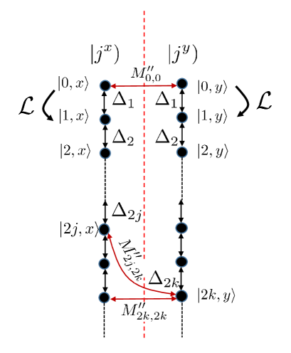
Figure 5: The orthonormal Krylov bases, Eq. (118), constructed for $B\!=\!0$ from $j^{x}$ and $j^{y}$ by repeated application of the Liouvillian ${\cal L}$. $\Delta_{n}$ are the recurrents of $\sigma_{xx}$. $M^{\prime\prime}_{n,m}={\mbox{Im}}\langle n/_{j^{x}}|{\cal M}|m/_{j^{y}}\rangle$ are the magnetization matrix elements used in Eq. (35).

Bogoliubov hyperspace is the Hilbert space of operators (hyperstates) $|A),|B)$. The inner product given by Eq. (10) depends on the Hamiltonian $H$ and inverse temperature $\beta$ and can be written in several forms

$$(A|B) = \sum_{nm}{\rho_{n}-\rho_{m}\over E_{m}-E_{n}}\langle m|A^{\dagger}|n\rangle\langle n|B|m\rangle,$$ (114)

$$= -\partial_{h_{A}}\partial_{h_{B}}{\mbox{Tr}}\log e^{-(\beta H-h_{A}A-h_{B}B)}\Big{|}_{h_{A},h_{B}\!=\!0},$$

$$= \int_{0}^{\beta}d\tau\langle A(\tau)B\rangle.$$

The first line can be used to confirm that $(A|B)=(B|A)^{*}$ and $(A|A)\geq 0$. The second line shows that $(A|B)$ is an equilibrium susceptibility obtained by adding static source terms $-h_{A}A-h_{B}B$ to $H$ before differentiation. The third line relates the inner product to an imaginary time correlation function. Here, $\langle O\rangle\equiv{\mbox{Tr}}\rho O$, and $A(\tau)\equiv e^{H\tau}Ae^{-H\tau}$. Where possible, $(A|B)$ could be computed by imaginary time quantum Monte Carlo algorithms prokofiev ; assaad .

The Liouvillian is a hermitain hyperoperator

$${\cal L}|A)=|[H,A]).$$ (115)

The hyperresolvent requires an ”$i{\varepsilon}$” prescription, which defines the hermitian and antihermitian parts as

$$\left({1\over{\cal L}-\omega-i{\varepsilon}}\right)\equiv\left({1\over{\cal L}-\omega}\right)^{\prime}+i\left({1\over{\cal L}-\omega}\right)^{\prime\prime}$$

$$\equiv\left({{\cal L}-\omega\over({\cal L}-\omega)^{2}+{\varepsilon}^{2}}\right)+i\left({{\varepsilon}\over({\cal L}-\omega)^{2}+{\varepsilon}^{2}}\right).$$ (116)

According to Eq. (8) we must keep ${\varepsilon}>0$ as we take $V\to\infty$.

We construct an orthonormal Krylov basis of operators, which will allow a matrix representation of the Liouvillian and its inverse. We start with the normalized root state

$$|0/_{A}\rangle\equiv{|A)\over\sqrt{(}A|A)},$$ (117)

where $A$ is the root operator (i.e. the uniform electrical or thermal current, in this paper).

Assuming $A$ is not in the kernel of ${\cal L}$, we construct the Krylov basis as follows

$$|1/_{A}\rangle = {\cal L}|0/_{A}\rangle,$$

$$|n/_{A}) \equiv (1-{\cal P}_{n-2}){\cal L}(1-{\cal P}_{n-3}){\cal L}\cdots(1-{\cal P}_{0}){\cal L}^{2}|0/_{A}\rangle,$$

$$|n/_{A}\rangle = N_{n}|n/_{A}),$$

$$N_{n} = {1\over\sqrt{(n/_{A}|n/_{A})}},$$ (118)

where ${\cal P}_{n}=|n/_{A}\rangle\langle n/_{A}|$.

It is easy to verify that the Krylov basis is orthonormal

$$\langle n/_{A}|m/_{A}\rangle=\delta_{mn}$$ (119)

and can be used to span the subspace ${\cal S}_{A}=\{{\cal L}^{n}|A)\}_{n=0}^{\infty}$ by the resolution of identity in the subspace ${\cal S}_{A}$

$$\sum_{n=0}^{\infty}|n/_{A}\rangle\langle n/_{A}|=1_{{\cal S}_{A}}.$$ (120)

Henceforth, we drop the label “$/_{A}$” in the hyperstates, unless needed.

The matrix representation of the Liouvillian in this Krylov basis is

$$\langle n|{\cal L}|m\rangle\equiv L_{nm}=\left(\begin{array}[]{cccc}0&\Delta_{1}&0&\ldots\\ \Delta_{1}&0&\Delta_{2}&\ldots\\ 0&\Delta_{2}&0&\\ \vdots&\vdots&&\ddots\end{array}\right)_{nm},$$ (121)

where $\Delta_{n},n=1,2,\ldots$ are the recurrents, which are calculated in Appendix C.

If both $A$ and $B$ are either hermitian or antihermitian, $(A|B)$ is purely real. If we choose $A$ to be hermitian, ${\cal L}^{2j}A$ (${\cal L}^{2j+1}A$) is hermitian (antihermitian) for $j=0,1,\ldots$. Hence, $|2j\rangle$ ($|2j+1\rangle$) are hermitian (antihermitian), and $\Delta_{n}=\langle n+1|{\cal L}|n\rangle$ are purely real.

The Liouvillian Green function $\langle n|\left({1\over{\cal L}-z}\right)|m\rangle$ is the inverse of a tridiagonal matrix

$$G_{n,m}(z) = -\langle n|\left({1\over z-{\cal L}}\right)|m\rangle,$$ (126)

$$= \left(\begin{array}[]{cccc}-z&\Delta_{1}&0&\ldots\\ \Delta_{1}&-z&\Delta_{2}&\ldots\\ 0&\Delta_{2}&-z&\\ \vdots&\vdots&&\ddots\end{array}\right)^{-1}_{n,m}.$$

Appendix B Continued Fraction of Longitudinal Conductivities

The $(0,0)$ value of Eq. (126) is an infinite continued fraction

$$G_{0,0}(z)=-{1\over z-{\Delta_{1}^{2}\over z-{\Delta_{2}^{2}\over z-{\Delta_{3}^{2}\over\vdots}}}}.$$ (127)

The dynamical longitudinal dynamical conductivities are given by

$$\sigma_{\alpha\alpha}(\omega) \equiv \hbar\mu^{\alpha}_{0}~{}G^{\prime\prime}(\omega)_{0,0},$$ (128)

$$= -\hbar\omega{\mbox{Im}}{1\over\hbar\omega+i{\varepsilon}-{|\Delta_{1}|^{2}\over\hbar\omega+i{\varepsilon}-{|\Delta_{2}|^{2}\over\hbar\omega+i{\varepsilon}-{\over\vdots}}}}.$$

where

$$\mu_{0} = {1\over{\cal V}}(j^{x}|j^{x})=\int_{-\infty}^{\infty}\!{d\omega\over 2\pi}\sigma_{xx}(\omega),$$

$$\mu^{Q}_{0} = {1\over{\cal V}}(j_{Q}^{x}|j^{x}_{Q})=\int_{-\infty}^{\infty}\!{d\omega\over 2\pi}\kappa_{xx}(\omega)$$ (129)

are the zeroth moments (sum rules) of the conductivity and the thermal conductivity respectively.

For continuum particles of charge $q$, mass $m$, and density $n$

$$\mu_{0}={1\over\hbar V}{\mbox{Tr}}\rho[P^{x},j^{x}]={nq^{2}\over m},$$ (130)

which is known as the f-sum rule. The thermal conductivity sum rule is given by Eq. (13) as

$$\mu_{0}^{Q}={1\over\hbar V}{\mbox{Tr}}\rho[Q^{x},j_{Q}^{x}].$$ (131)

This sum rule was introduced as $\Theta_{xx}/T$ and evaluated by Shastry shastry-sumrules for certain models.

The DC order of limit (8) of (132) is

$$\sigma_{xx} = {\mbox{Im}}{-\hbar\mu_{0}\over i{\varepsilon}-{|\Delta_{1}|^{2}\over i{\varepsilon}-{|\Delta_{2}|^{2}\over i{\varepsilon}-{\over\vdots}}}},$$

$$\kappa_{xx} = {1\over T}{\mbox{Im}}{-\hbar\mu^{Q}_{0}\over i{\varepsilon}-{|\Delta^{Q}_{1}|^{2}\over i{\varepsilon}-{|\Delta^{Q}_{2}|^{2}\over i{\varepsilon}-{\over\vdots}}}}.$$ (132)

Appendix C Computing recurrents from moments

Here we show how the recurrents $\Delta_{n},\Delta_{n}^{Q},~{}n=1,2,\ldots$ can be computed recursively from their respective moments, which are equilibrium averages of operators. The conductivity is an even function of frequency, and it has only even moments $\mu_{2k}$. For $k>0$, the moments are given by equilibrium averages

$$\mu_{2k} = {1\over{\cal V}}\langle j|{\cal L}^{2k}|j)=\left(L^{2k}[\Delta]\right)_{0,0},$$ (133)

$$= {1\over{\cal V}}{\mbox{Tr}}\rho\left[j,{\cal L}^{2k-1}j\right].$$

$L$ is the tridiagonal matrix given in Eq. (121). By taking the $(0,0)$ matrix elements of even powers $L[\Delta]$, an algebraic recursive relation is obtained between the moments and recurrents

$${\mu_{2}\over\mu_{0}} = \Delta_{1}^{2},$$

$${\mu_{4}\over\mu_{0}} = \Delta_{1}^{2}(\Delta_{1}^{2}+\Delta_{2}^{2}),$$

$${\mu_{6}\over\mu_{0}} = \Delta_{1}^{2}\left(\Delta_{1}^{4}+2\Delta_{1}^{2}\Delta_{2}^{2}+\Delta_{2}^{4}+\Delta_{2}^{2}\Delta_{3}^{3}\right),$$

$$\vdots = \vdots,$$ (134)

which can readily be inverted to obtain the lowest $k=1,2,\ldots k_{\rm max}$ recurrents from the lowest $k_{\rm max}+1$ moments

$$\Delta_{1}^{2} = \mu_{2}\over\mu_{0},$$

$$\Delta_{2}^{2} = {\mu_{4}\over\mu_{0}\Delta_{1}^{2}}-\Delta_{1}^{2},$$

$$\Delta_{3}^{2} = {\mu_{6}\over\mu_{0}\Delta_{1}^{2}\Delta_{2}^{2}}-{\Delta_{1}^{4}\over\Delta_{2}^{2}}-2\Delta_{1}^{2}-\Delta_{2}^{2},$$

$$\vdots = \vdots.$$ (135)

Note: a useful relation exists between the recurrents $\Delta_{i},i\leq n$ and the normalization constants $N_{n}$ in Eq. (118)

$$N_{n}=\prod_{i=1}^{n}{1\over|\Delta_{i}|}.$$ (136)

Appendix D Variational Extrapolation of Recurrents

Any calculation of a finite set of recurrents $\Delta_{n},n\leq n_{\rm max}$ is not sufficient for determining Eq. (127). An infinite extrapolation of $\{\Delta_{n^{\prime}}\}_{n_{\rm max}+1}^{\infty}$ is required.

Several extrapolation schemes have been proposed. The Variational Extrapolation of Recurrents (VER) Sandvik ; lindner ; khait has been found to be reliable in certain cases. VER chooses a physically-motivated variational function $\sigma^{\rm ver}(\omega;\{\alpha_{i},i=1,\ldots\})$ with sufficiently many variational parameters. $\alpha_{i}^{\rm ver}$ are determined by a least-squares fit between the recurrents of $\sigma^{\rm ver}$ and the computed set. The conductivity is then approximated by,

$$\sigma_{\alpha\alpha}(\omega)\approx-{\mbox{Im}}\cfrac{\hbar\mu_{0}}{\hbar\omega+i{\varepsilon}-\cfrac{\Delta_{1}^{2}}{\hbar\omega+i{\varepsilon}-\cfrac{\Delta_{2}^{2}}{\cfrac{\ddots}{\hbar\omega+i{\varepsilon}-\cfrac{|\Delta_{n_{\rm max}-1}|^{2}}{\hbar\omega+i{\varepsilon}-|\Delta_{n_{\rm max}}|^{2}T^{\rm ver}(\omega)}}}}},$$ (137)

where $T^{\rm ver}(\omega)$ is a complex termination function, which is “borrowed” from the fitted variational function $\sigma^{\rm ver}(\omega)$. The reliability of the VER procedure is in principle testable by finding convergence as $n_{\rm max}$ is incrementally increased.

Appendix E Off-diagonal Green functions

To prove Eq. (LABEL:HallN) we need to determine $G_{n,m}(i{\varepsilon})=G^{\prime}_{n,m}+iG^{\prime\prime}_{n,m}$ in Eq. (126). Due to the tridiagonal properties of $L$ and the conditions $(G^{\prime}+iG^{\prime\prime})L=L(G^{\prime}+iG^{\prime\prime})=I$, the following properties follow

$$G_{n,m}=G_{m,n},$$

$$G_{2i,2j+1}=G^{\prime}_{2i,2j+1}={\rm real},$$

$$G_{2i,2j}=iG^{\prime\prime}_{2i,2j}={\rm imaginary},$$

$$G_{2i+1,2j+1}=0.$$ (138)

In particular, we see that for any $|n\rangle$

$${\mbox{Im}}G_{1,n}=\langle 1\Big{|}\left({1\over{\cal L}}\right)^{\prime\prime}\Big{|}n\rangle=0.$$ (139)

Hence, one can write

$$\left({1\over{\cal L}}\right)^{\prime\prime}{\cal L}j^{x}=0,$$ (140)

which proves Eq. (33).

The nonzero imaginary Green function can be written as

$$G^{\prime\prime}_{2k,0}=G^{\prime\prime}_{0,2k}=R_{k}G^{\prime\prime}_{0,0},$$

$$R_{k}\equiv\prod_{j=1}^{k}\left(-{\Delta_{2j-1}\over\Delta_{2j}}\right).$$ (141)

By Eq. (132)

$$\sigma_{xx}(0)=-\hbar\mu_{0}G^{\prime\prime}_{0,0},$$ (142)

where $\mu_{0}=(j^{x}|j^{x})/{\cal V}$. Thus, by Eq. (138), all the odd entries drop out of the sums in Eq. (LABEL:HallN), and $\sigma_{xx}^{2}$ factors out of the sums. Therefore, the dissipative longitudinal conductivity is completely eliminated from the Hall coefficient formula, which is left to depends solely on thermodynamical susceptibilities.

References

- [1] H. Jones. H. Jones and C. Zener, Proc. Roy. Soc.(London), 145, 268 (1934).
- [2] J. M. Ziman. Electrons and phonons: the theory of transport phenomena in solids. Oxford university press, (1960).
- [3] N. P. Ong. Geometric interpretation of the weak-field hall conductivity in two-dimensional metals with arbitrary fermi surface. Phys. Rev. B, 43,193- (1991).
- [4] Anisotropy of relaxation times on the Fermi surface effects the Hall coefficient [2, 3]. Neverthelss, formula (2) with its correction term is an equilibrium expression which includes the effects of scattering anisotropy. See discussion after Eq. (72).
- [5] Equilibrium expressions for non-metallic (i.e. zero resistivity) phases are the Streda formula and Chern number for the Hall conductivity, which will be discussed in Section VII.
- [6] V. J. Emery and S. A. Kivelson. Superconductivity in bad metals. Phys. Rev. Lett., 74,3253 (1995).
- [7] N. H. Lindner and A. Auerbach. Conductivity of hard core bosons: a paradigm of a bad metal. Phys. Rev. B 81, 054512, 2010.
- [8] A. W. Smith, T. W. Clinton, C. C. Tsuei, and C. J. Lobb. Sign reversal of the hall resistivity in amorphous mo 3 si. Phys. Rev. B, 49, 12927 (1994).
- [9] X. Zhang, Q. Yang, A. Palevski, and A. Kapitulnik. Superconductor-insulator transition in indium oxide thin films. Bulletin of the American Physical Society, (2018).
- [10] S. J. Hagen, C. J. Lobb, R. L. Greene, M. G. Forrester, and J. H. Kang. Anomalous hall effect in superconductors near their critical temperatures. Phys. Rev. B, 41, 11630 (1990).
- [11] S. Badoux, W. Tabis, F. Laliberté, G. Grissonnanche, B. Vignolle, D. Vignolles, J. Béard, D. A. Bonn, W. N. Hardy, R. Liang, N. Doiron-Leyraud, L. Taillefer, and C. Proust. Change of carrier density at the pseudogap critical point of a cuprate superconductor. Nature, 531, 210 (2016).
- [12] L. Klein, J.S. Dodge, C.H. Ahn, J.W. Reiner, L Mieville, T.H. Geballe, M.R. Beasley, and A. Kapitulnik. Transport and magnetization in the badly metallic itinerant ferromagnet. Journal of Physics: Condensed Matter, 8, 10111 (1996).
- [13] Assa Auerbach. Hall number of strongly correlated metals. Phys. Rev. Lett., 121, 066601, (2018).
- [14] C. Domb. Phase transitions and critical phenomena, Vol 3,, volume 19. Elsevier, (2000).
- [15] U. Schollwock. The density-matrix renormalization group in the age of matrix product states. Annals of Physics, 326(1), 96 (2011). January 2011 Special Issue.
- [16] N. Prokof’ev and B. Svistunov. Worm algorithms for classical statistical models. Phys. Rev. Lett., 87,160601 (2001).
- [17] F. F. Assaad. Phase diagram of the half-filled two-dimensional SU(N) Hubbard-Heisenberg model: A quantum Monte Carlo study. Phys. Rev. B, 71, 075103 (2005).
- [18] Real-time dissipative response functions suffer from Suzuki-Trotter errors at long times [19], ill-posed analytical continuation at finite temperatures [20, 21], or extrapolation of moments to infinite order [31, 7, 33]. see appendix (D) for a review of such an extrapolation.
- [19] S.R. White and A.E. Feiguin. Real-time evolution using the density matrix renormalization group. Phys. Rev. Lett., 93,076401, (2004).
- [20] M. Jarrell and J. E. Gubernatis. Bayesian inference and the analytic continuation of imaginary-time quantum monte carlo data. Physics Reports, 269, 133 (1996).
- [21] S. Gazit, D. Podolsky, A. Auerbach, and D.P. Arovas. Dynamics and conductivity near quantum criticality. Phys. Rev. B, 88, 235108 (2013).
- [22] K. Behnia and H. Aubin. Nernst effect in metals and superconductors: a review of concepts and experiments. Reports on Progress in Physics, 79(4),046502 (2016).
- [23] B. Sriram Shastry. Sum rule for thermal conductivity and dynamical thermal transport coefficients in condensed matter. Phys. Rev. B, 73, 085117 (2006).
- [24] N. N. Bogoliubov. Dubna Report, 1962.
- [25] N. D. Mermin and H. Wagner. Absence of ferromagnetism or antiferromagnetism in one- or two-dimensional isotropic heisenberg models. Phys. Rev. Lett., 17, 1133 (1966).
- [26] H. Mori. Transport, collective motion, and brownian motion. Progress of Theoretical Physics, 33, 423 (1965).
- [27] D. Forster. Hydrodynamic fluctuations, broken symmetry, and correlation functions, Ch. V. CRC Press, (2018).
- [28] R. Zwanzig. Nonequilibrium statistical mechanics. Oxford University Press, (2001).
- [29] W. Götze and P. Wölfle. Homogeneous dynamical conductivity of simple metals. Phys. Rev. B, 6, 1226, (1972).
- [30] M. Howard Lee, J. Hong, and J. Florencio Jr. Method of recurrence relations and applications to many-body systems. Physica Scripta, 1987, 498, (1987).
- [31] V. S. Viswanath and G. Müller. The Recursion Method: Application to Many Body Dynamics, volume 23. Springer Science & Business Media, (1994).
- [32] O. A. Starykh, A. W. Sandvik, and R. R. P. Singh. Dynamics of the spin-heisenberg chain at intermediate temperatures. Phys. Rev. B, 55, 14953, (1997).
- [33] I. Khait, S. Gazit, N. Y. Yao, and A. Auerbach. Spin transport of weakly disordered heisenberg chain at infinite temperature. Phys. Rev. B, 93, 224205 (2016).
- [34] P. Streda and L. Smrcka. Thermodynamic derivation of the hall current and the thermopower in quantising magnetic field. Journal of Physics C: Solid State Physics, 16, L895, (1983).
- [35] A. H. MacDonald and P. Steda. Quantized hall effect and edge currents. Phys. Rev. B, 29,1616, (1984).
- [36] D. J. Thouless, M. Kohmoto, M. P. Nightingale, and M. den Nijs. Quantized hall conductance in a two-dimensional periodic potential. Phys. Rev. Lett., 49, 405 (1982).
- [37] J. E. Avron and R. Seiler. Quantization of the hall conductance for general, multiparticle schrödinger hamiltonians. Phys. Rev. Lett. , 54, 259 (1985).
- [38] S. D. Huber and N. H. Lindner. Topological transitions for lattice bosons in a magnetic field. Proceedings of the National Academy of Sciences, 108, 19925 (2011).
- [39] A. Dauphin and N. Goldman. Extracting the chern number from the dynamics of a fermi gas: Implementing a quantum hall bar for cold atoms. Phys. Rev. Lett., 111,135302 (2013).
- [40] P. Prelovšek, M. Long, T. Markež, and X. Zotos. Hall constant of strongly correlated electrons on a ladder. Phys. Rev. Lett., 83, 2785 (1999).
- [41] M. Aidelsburger, M. Lohse, C. Schweizer, M. Atala, J. T. Barreiro, S. Nascimbene, N. R. Cooper, I. Bloch, and N. Goldman. Measuring the chern number of hofstadter bands with ultracold bosonic atoms. Nature Physics, 11, 162, 2015.
- [42] N. R. Cooper, B. I. Halperin, and I. M. Ruzin. Thermoelectric response of an interacting two-dimensional electron gas in a quantizing magnetic field. Phys. Rev. B, 55,2344 (1997).
- [43] The derivation below is simpler and more general than in Ref. [13]. The primary difference is the use of polarizations operators, which mutually commute, and are independent of magnetic field.
- [44] R. J. Hardy. Energy-flux operator for a lattice. Phys. Rev., 132,168 (1963).
- [45] J. R. Schrieffer and P. A. Wolff. Relation between the anderson and kondo hamiltonians. Phys. Rev., 149, 491 (1966).
- [46] A. Auerbach. Interacting electrons and quantum magnetism. Springer Science & Business Media (2012).
- [47] C. J. Morningstar and M. Weinstein. Contractor renormalization group technology and exact hamiltonian real-space renormalization group transformations. Phys. Rev. D, 54, 4131 (1996).
- [48] E. Altman and A. Auerbach. Plaquette boson-fermion model of cuprates. Phys. Rev. B, 65, 104508 (2002).
- [49] S. Capponi, V.R. Chandra, A. Auerbach, and M. Weinstein. p 6 chiral resonating valence bonds in the kagome antiferromagnet. Phys. Rev. B, 87, 161118 (2013).
- [50] K. Behnia. Fundamentals of thermoelectricity. OUP Oxford, 2015.
- [51] M. P. A. Fisher, P. B. Weichman, G. Grinstein, and Daniel S. Fisher. Boson localization and the superfluid-insulator transition. Phys. Rev. B, 40, 546 (1989).
- [52] B. S. Shastry, B. I. Shraiman, and R. R. P. Singh. Faraday rotation and the hall constant in strongly correlated fermi systems. Phys. Rev. Lett. , 70, 2004 (1993).
- [53] The minimal coupling is consistent with the sign of the density-phase commutator.
- [54] M. Jonson and S.M. Girvin. Thermoelectric effect in a weakly disordered inversion layer subject to a quantizing magnetic field. Phys. Rev. B, 29,1939 (1984).
- [55] A weaker condition for reversing the order of limits, is local incompressibility [66]. that is to say, the charge and flux densities (both coarse grained quantities on some microscopic correlation length) should be “locally locked” , and similarly, .
- [56] N. Lindner, A. Auerbach, and D. P. Arovas. Vortex dynamics and hall conductivity of hard-core bosons. Phys. Rev. B, 82,134510 (2010).
- [57] E. Berg, S. D. Huber, and N. H. Lindner. Sign reversal of the hall response in a crystalline superconductor. Phys. Rev. B, 91, 024507 (2015).
- [58] A. Auerbach. Comparison of tunneling rates of fractional charges and electrons across a quantum hall strip. Phys. Rev. Lett. , 80, 817 (1998).
- [59] I. Khait and A. Auerbach. Hall number of the t-J model. Manuscript in preparation.
- [60] A. C. Hewson. The Kondo problem to heavy fermions, volume 2. Cambridge university press, (1997).
- [61] X. Wan, A. Turner, A. Vishwanath, and S. Y. Savrasov. Topological semimetal and fermi-arc surface states in the electronic structure of pyrochlore iridates. Phys. Rev. B, 83(20),205101 (2011).
- [62] H. Fukuyama. Effects of intervalley impurity scattering on the non-metallic behavior in two-dimensional systems. Journal of the Physical Society of Japan, 49(2),649 (1980).
- [63] B. L. Altshuler, D. Khmel’nitzkii, A. I. Larkin, and P. A. Lee. Magnetoresistance and hall effect in a disordered two-dimensional electron gas. Phys. Rev. B, 22, 5142 (1980).
- [64] B. Shapiro and E. Abrahams. Scaling theory of the hall effect in disordered electronic systems. Phys. Rev. B, 24, 4025 (1981).
- [65] E. Shimshoni and A. Auerbach. Quantized hall insulator: Transverse and longitudinal transport. Phys. Rev. B, 55, 9817 (1997).
- [66] A. H. MacDonald and P. Steda. Quantized hall effect and edge currents. Phys. Rev. B, 29, 1616 (1984).