Mode Classification in Fast-Rotating Stars using a Convolutional Neural Network: Model-Based Regular Patterns in $\delta$ Scuti Stars

Abstract

Oscillation modes in fast-rotating stars can be split into several subclasses, each with their own properties. To date, seismology of these stars cannot rely on regular pattern analysis and scaling relations. However, recently there has been the promising discovery of large separations observed in spectra of fast-rotating $\delta$ Scuti stars: they were attributed to the island-mode subclass, and linked to the stellar mean density through a scaling law. In this work, we investigate the relevance of this scaling relation by computing models of fast-rotating stars and their oscillation spectra. In order to sort the thousands of oscillation modes thus obtained, we train a convolutional neural network isolating the island modes with 96% accuracy. Arguing that the observed large separation is systematically smaller than the asymptotic one, we retrieve the observational $\Delta\nu-\overline{\rho}$ scaling law. This relation will be used to drive forward modelling efforts, and is a first step towards mode identification and inversions for fast-rotating stars.

1 Introduction

1.1 Fast-rotating stars

Through space missions such as MOST, CoRoT and Kepler, asteroseismology has proven to be the most powerful tool by which to probe stellar interiors. Most of the results obtained through this technique rely on the regular patterns the mode frequencies follow, that can readily be linked to the stellar fundamental parameters through scaling laws. However, this technique works for slowly-rotating solar-like oscillators, where mode identification is possible. Deeper insight can be gained through the analysis of rotational splittings, automated inferences or inversion techniques. In fast-rotating stars, such identification is not so easy: while the centrifugal force distorts the stellar geometry, the Coriolis force complicates mode geometries such that they can no longer be described in terms of simple spherical harmonics. Currently, it is standard to use a linear combination of spherical harmonics as a basis to describe the modes, but this prevents mode identification in terms of the classical quantum numbers $(n,\ell,m)$.

1.2 Classes of modes

Theoretical works show that pressure modes in fast-rotating stars can be sorted in different categories. Lignières & Georgeot (2009) split pressure modes in fast-rotating stars in four sub-classes: 2-period island modes, 6-period island modes, whispering gallery modes and chaotic modes. Each of these subclasses has its own regular spacing in frequency. In measured spectra however, those spacings cannot readily be distinguished and the associated information on the stellar structure cannot easily be retrieved.
García Hernández et al. (2015, 2017) analyzed a sample of ten stars, and identified regular patterns in the their high-frequency spectra. They found a large frequency separation that they attribute to 2-period island modes, and linked this separation to the stellar mean density through a scaling law, as predicted by Reese et al. (2008). In this work, we provide further validation by exploring theoretical models and their oscillations to test the proposed scaling law.

2 Method

2.1 Codes

We compute rotating star models using the two-dimensional structure code ESTER (Rieutord & Espinosa Lara (2013), Rieutord et al. (2016)). Adiabatic oscillations of these models are calculated using TOP (Reese et al. (2009), Reese et al. in prep.). The geometry these codes use rely on the definition of a pseudoradius $\zeta$, that goes from 0 at the center of the star to 1 at the distorted stellar surface (see Bonazzola et al., 1998). The radial grid is split into eight Gauss-Lobatto-Chebyshev subgrids of 30 points, while the latitudinal components are projected on 24 spherical harmonics for the structure and 40 spherical harmonics for the oscillations. This resolution leads to 48,000 modes in the whole spectrum that are of potential interest.

2.2 Convolutional Neural Network Classifier

2.2.1 Network Architecture

Previously, mode sorting was performed manually through plotting and visually inspecting the TOP eigensolutions. Given that this task is essentially an image classification problem, the process can be automated through the use of a convolutional neural network (CNN). In the last few years machine learning algorithms have become more widely adopted in stellar astrophysics (Bellinger et al., 2016; Verma et al., 2016; Angelou et al., 2017) including CNNs (Hon et al., 2017).

We utilised Google’s Tensorflow libraries (Abadi et al., 2015) to create a seven layer, 2D-convolutional network for the purposes of classifying the TOP oscillation modes. We employ a network architecture comprising two convolution, two pooling and two fully connected layers supplemented by an output layer. A rectified linear unit activation function is applied to the convolution and fully-connected layers. Max-pooling is used to downsample the convolutions and drop out is employed as form of regularization for the fully-connected layers. A softmax function is used to activate the output layer for the purpose of assigning class probabilities.

Before applying the algorithm to mode classification in rapidly-rotating stars we conducted several tests of our CNN. We validated our network on the MNIST database of handwritten digits with 99.3% accuracy (Lecun et al., 1998). As per Hon et al. (2017), we classified the evolutionary phase of Kepler giants in the Vrard et al. (2016) sample with 98% accuracy.

2.2.2 Training and development set for mode classification

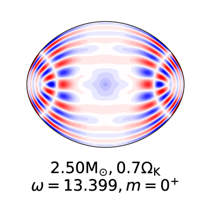
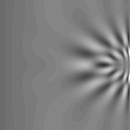
Figure 1: Island pressure mode at $(\widetilde{n},\widetilde{\ell},m)=(16,1,0)$, used in the training set. Left: meridional cross-section of the Eulerian pressure perturbation divided by the square root of the background density. Right: Same quantity plotted as a function of the pseudoradius $\zeta$ and the colatitude $\theta$.

To visualize the oscillations through the model, we represent the ratio of the Eulerian pressure perturbation to the square root of the background density; this quantity brings out surface variations. For visual inspection purposes, we plot this quantity along a meridional cross-section. We feed the algorithm 128x128 (pixels) grey scale images of the same quantity, plotted in the pseudoradius-colatitude $(\zeta,\theta)$ plane, for $\theta$ going from 0 to $\pi$. Figure 1 shows these two representations for a given oscillation.

To train the algorithm, we classify by eye 4300 modes divided into seven classes: (i) spurious modes, (ii) rosette g modes, (iii) subcritical g modes, (iv) g modes with some envelope extent, (v) whispering gallery p modes, (vi) island p modes of period 2, (vii) other p modes.

We only keep modes fitting the canonical description of the modes given by Lignières & Georgeot (2009), omitting mixed modes and modes resulting from avoided crossings. Although we do not exploit the whole set of available mode types, the sorted classes are sufficient for our purposes.

The 4300 images with known truth labels were divided into a training set (80%) and a development set (20%). We performed a 10-fold validation test which yielded a mean accuracy of 96% on randomly selected development sets. During the training process we optimized for 3000 iterations after which there was no significant improvement to our loss metric. We found that for the current application, the CNN was most responsive to the Adam optimizer. As our aim is to identify 2-period island modes, an accuracy of 96% was deemed satisfactory. False positives in this category could be discarded by eye. We note that there is scope to optimize the CNN performance further, and we will continue to do so in future work.

3 Regular patterns in the island-mode spectrum

3.1 Theoretical models and oscillations

We consider two series of ESTER models of 2.5 $M_{\odot}$ main-sequence stars: a series of ZAMS models for increasing rotation velocities and a series of models rotating at 70% of their Keplerian rotation rate with varying core hydrogen abundance $X_{c}$ to mimic main-sequence evolution.

Each of these models is computed for metallicities $Z=0.02$ and $Z=0.01$. These models cover the rotation and core abundance parameter space accessible for a $2.5M_{\odot}\ \delta$ Scuti star. Using the TOP code, we compute the adiabatic, even (symmetric with respect to the underlying ray path) axisymmetric ($m=0$) oscillations of these models. We consider a high frequency interval, where we expect mostly pressure modes, and find about 500 modes in the chosen range for each model. These modes are then fed into the convolutional neural network described in section 2.2.1, keeping the modes identified with a probability of 95%.

3.2 Comparison with the observations

Island modes of period 2 are known to be the rotating counterpart of low-degree pressure modes (Pasek et al., 2012). In order to identify and study these modes, we use the description from Reese et al. (2009): each island mode is described using three quantum numbers, $\widetilde{n},\widetilde{\ell},m$. The first two quantities are illustrated on figure 1: $\widetilde{n}$ is the number of nodes along the wave train from the two points where it reaches the surface, while $\widetilde{\ell}$ being the number of parallels (i.e. the number of nodal lines parallel to the equator) from pole to equator. The azimuthal order $m$ does not change definition with respect to the non-rotating case, and is equal to the periodicity in the azimuthal direction.

Lignières & Georgeot (2009) described the island modes in a polytropic rotating fluid, and highlighted regular patterns in their frequency spectra. Successive modes at a given value of $\widetilde{\ell}$ are separated by a frequency distance that reaches an asymptotic value for high-frequency modes: this value is usually called the large separation.

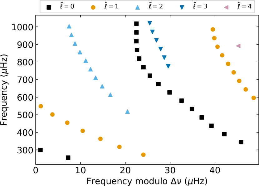
Figure 2: Identification of island modes obtained through our neural network for a $Z=0.02$, 2.5 $M_{\odot}$ model rotating at 70% of its breakup velocity, with 60% of its initial hydrogen abundance in the core. Here, $\Delta\nu=49.78\mu$Hz in the asymptotic regime.

Figure 2 shows an échelle diagram for one of the models we examined. Each ridge corresponds to a different value of $\widetilde{\ell}$ (obtained here through visual inspection). A regular separation appears and stabilizes when reaching the high-frequency asymptotic regime, thus confirming the result obtained on polytropic models by Lignières & Georgeot (2009).

García Hernández et al. (2015, 2017) analyzed observed oscillation spectra for several rotating $\delta$ Scuti stars. They identified statistically significant patterns in the frequency spectra. They were then able to correlate these large separations with the mean density of the star through a power law that reads:

$$\frac{\overline{\rho}}{\overline{\rho}_{\odot}}=1.55^{+1.07}_{-0.68}\left(\frac{\Delta\nu}{\Delta\nu_{\odot}}\right)^{2.035\pm 0.095},$$ (1)

with $\overline{\rho}_{\odot}=1.41$ g/cm³ and $\Delta\nu_{\odot}=134.8\mu Hz$ (Kjeldsen et al., 2008)

From our models, we obtain a similar scaling law in the asymptotic regime, that is

$$\frac{\overline{\rho}}{\overline{\rho}_{\odot}}=1.22\pm 0.02\left(\frac{\Delta\nu}{\Delta\nu_{\odot}}\right)^{2.091\pm 0.02}.$$ (2)

Note that the errorbars in equation 1 are observational, while those of equation 2 come from the fitting process. While the coefficients in our relation fall within the uncertainties of the observational relation, we find a difference in the constant factor (corresponding to the offset between the two trends in fig. 3).

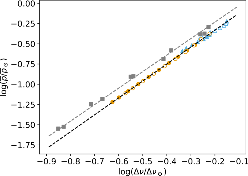
Figure 3: Stellar mean density as a function of the island-mode large separation computed in the asymptotic regime. Coloured data points are from our calculations. Empty symbols are for $Z=0.01$ and filled symbols for $Z=0.02$. Blue triangles correspond to varying rotational velocities, orange circles to varying hydrogen core abundances. The black dotted line is our fit using all our models. The grey squares are the data points and the grey dashed line is the corresponding fit from García Hernández et al. (2017).

3.2.1 Effect of the metallicity

The stars observed by García Hernández et al. (2017) have metallicities in the range $Z\sim 0.008-0.02$, which is covered by our models at $Z=0.01$ or $Z=0.02$. As can be seen on figure 3, models at $Z=0.01$ tend to be slightly denser than their $Z=0.02$ counterparts. However, the large separation derived from their island-mode spectrum follows closely the same scaling law: the metallicity variations in the (narrow) range corresponding to the observations has no impact on the $\overline{\rho}-\Delta\nu$ relation.

3.2.2 Roche model

Mean densities for eclipsing binary stars are derived by computing Roche model surfaces, which rely on the simplifying assumptions that the stellar mass is concentrated in its center and is rotating uniformly. The stellar volume is computed supposing, for simple geometrical reasons, that the radius measured through the eclipse analysis is the equatorial one. In order to test these assumptions and their impact on the estimate of the volume, we compute the volume of both the ESTER model and a Roche model of the same equatorial radius.

The volume of a given ESTER model is obtained through the integral

$$V=\iiint r^{2}\sin\theta d\theta d\phi dr=4\pi\int^{\pi/2}_{0}\frac{R_{s}^{3}(\theta)}{3}\sin\theta d\theta,$$ (3)

where $R_{s}$ is the surface radius computed consistently with the distribution of matter inside the star.

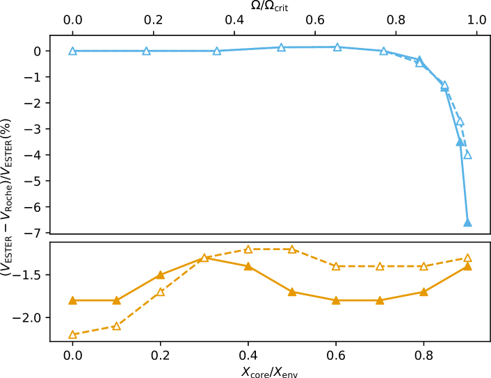
Figure 4: Relative difference in volume between Roche and ESTER models, in percentage, as a function of the rotation rate (top panel) or the core hydrogen abundance (bottom panel). The symbols are the same as in figure 3. The negative values show that Roche models tend to systematically underestimate the stellar volume, compared to ESTER models.

Figure 4 shows the relative difference $\Delta{\rm Volume}$, defined as $\left(\rm{V(Roche)-V(ESTER)}\right)/\rm V(ESTER)$. We find a systematic difference: Roche models always underestimate the volume, compared to models allowing for a more realistic distribution of matter and rotation profile. We see that the volume is underestimated by $\sim 1.6$% on average, and does not seem to depend on the model core hydrogen abudance. It remains low for all models, except at the most extreme rotation rate (at 90% of the critical velocity, where the difference can reach 6.6%). While this difference may impact the determination of stellar mean densities and interferometric radii, for instance, it still is one order of magnitude too small to account for the offset between the scaling relations eq. (1) and eq. (2).

3.2.3 Below the asymptotic regime

We contend that the discrepancy between the scaling relation obtained through modelling and that inferred from the observations lies with the frequency regime in which we compute the large separation. Indeed, in order to compare our results with the predictions of Lignières & Georgeot (2009), we computed high-frequency modes so to place ourselves in the asymptotic regime, where the large separation is expected to be constant.

However, García Hernández et al. (2009) showed that the frequency domain in which stars are observed is far below the asymptotic domain. They also showed that the large frequency separation increases with frequency: the leftward drift of the ridges shown in figure 2 is a signature of this phenomenon. Their calculations show that computing the large separation in the asymptotic domain can lead to a 10 to 15% overestimate with respect to the observations.

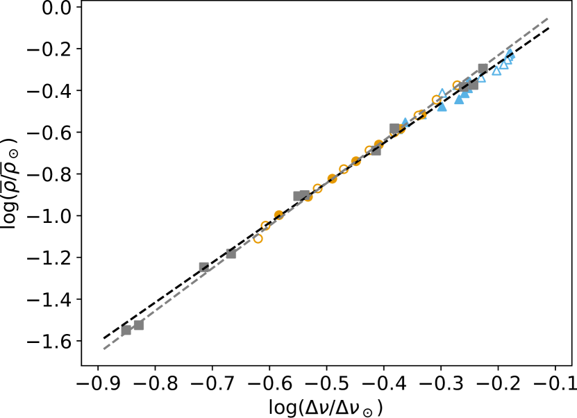
Figure 5: Stellar mean density as a function of the island-mode large separation in the frequency range corresponding to observations. Symbols are identical to those of figure 3.

To investigate this explanation, we compute island modes at lower frequencies. The stars observed by García Hernández et al. (2017) pulsate in different frequency ranges, that we compare to the breakup rotation rate of each star: those pulsation domains overlap in the range of $6$ to $9$ times the equatorial Keplerian velocity. The island modes in this range have orders $\widetilde{n}=8-12$, these values are consistent with the range of excitable modes predicted by Dupret et al. (2005) (note that, for even $\tilde{\ell}=0,m=0$ modes, $\tilde{n}=2n$). In comparison, the asymptotic regime is reached at frequencies roughly three times larger in our models, for $\tilde{n}=32-40$.

Figure 5 shows the separation computed in this domain, and qualitative agreement. The corresponding trend follows the relation

$$\frac{\overline{\rho}}{\overline{\rho}_{\odot}}=1.30\pm 0.06\left(\frac{\Delta\nu}{\Delta\nu_{\odot}}\right)^{1.905\pm 0.03}.$$ (4)

We find that the relation obtained using island modes fits the observations better than that computed in the asymptotic regime. The small difference with the observed relation may come from the reduced number of models we used. Indeed, not all the models we computed were included, as numerical errors prevented us from finding enough low-frequency island modes to compute a reliable separation in the most evolved cases. A wider domain in densities could be explored by computing models of different masses.

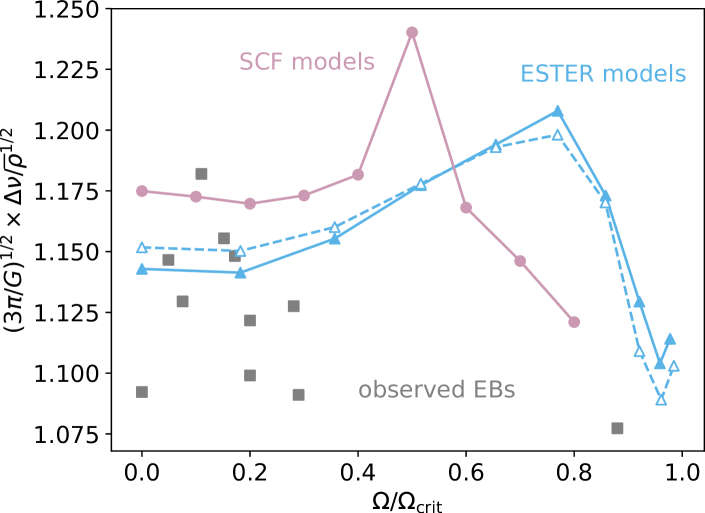
Figure 6: $\Delta\nu/\sqrt{\overline{\rho}}$ as a function of the rotation velocity (in units of the critical velocity). We use the values of $\Delta\nu$ obtained outside of the asymptotic (as in figure 5). We show the values obtained with $Z=0.02$ and $Z=0.01$ ESTER models (full blue symbols and solid line, and empty blue symbols and dashed line, respectively), and compare them with SCF models from Reese et al. (2009) (purple, see main text) and the observations from García Hernández et al. (2017) (grey). The lack of a clear trend confirms that the scaling does not depend explicitly on rotation.

In Figure 6 we plot the ratio $\Delta\nu/\sqrt{(}\overline{\rho})$ as a function of the rotation velocity. It shows the results obtained from ESTER models, along with simpler $2M_{\odot}$ SCF models (Reese et al., 2009) and observational data (García Hernández et al., 2017). In order to match the results for ESTER models, the data points for SCF models have been recomputed in the frequency domain corresponding to observations (the outlier at $\Omega=0.5\Omega_{\rm crit}$ is due to an avoided crossing between some of the computed modes). Some differences can be expected between the results for ESTER and SCF models, given that the former fully solve the structural and energy conservation equations, thus resulting in a 2D rotation profile and a baroclinic structure, whereas the latter only solves a horizontal average of the energy equation and uses imposed cylindrical (or in our case, uniform) rotation profiles, thus resulting in a simpler barotropic stellar structure. Nonetheless, the differences on $\Delta\nu$ remain relatively small. The lack of a trend with rotation shows that rotation has no additional impact on the large separation.

4 Conclusions

4.1 Summary

In this work, we computed two-dimensional models of fast-rotating stars and the corresponding oscillations by interfacing the ESTER and TOP codes. In order to compare to observations and conduct scientific analysis, it was necessary to first sort through the numerous modes calculated for every model. We trained a CNN to automate this process and classified the modes based on their geometry. Our network architecture was designed to be versatile and allowed us to achieve high accuracy whilst expediting the process dramatically.

In this first application of the deep-learning classification algorithm, we focused on identifying a specific subclass of pressure modes present in fast rotators, namely island modes of period 2. Those modes are expected to be the most visible in the p-mode frequency range, and to follow regular frequency patterns in the high-frequency asymptotic regime. We recover such patterns with state-of-the-art models, confirming both previous theoretical and observational works. Previous work has linked the large frequency separation of observed modes with the stellar mean density through a scaling law. We find a similar relation using the island-mode large separation, with an offset. We find that this difference cannot be attributed to metallicity effects nor to the estimate of the stellar volume, but arises from ‘the difference in the frequency domain sampled by the observed modes and the asymptotic domain in which we study the synthetic oscillations. Indeed, the modes observed in actual stars are not in the asymptotic regime and therefore present large separations roughly 10% smaller: this difference can also be used to obtain an estimate of the radial order of the detected oscillations in a given star. This $\overline{\rho}-\Delta\nu$ relation obtained from the observations is a very useful guide in modelling p-mode pulsators, such as $\delta$ Scuti stars, and will in turn help mode identification and the matching between models and observed stars.

4.2 Future prospects

We note that there is scope to optimize the CNN performance further, and we will continue to do so in future work. We can also modify the CNN to use quarter-plane plots, thus increasing the density of pixels by a factor of 2. Such an improvement would require the creation of separate training sets for the odd and even modes, which we are developing for future work.

Once the CNN had identified the 2-period island modes, they were manually sorted according to their spherical degree $\widetilde{\ell}$. This subsequent classification step can also be automated with a CNN and indeed the current work has provided us with a substantial training set to do so. We report an accuracy of $>$99% from our validation tests and have since added this automated classification step in our analysis pipeline for future use.

Exploring a wider range of models, varying other parameters (and most notably the stellar mass) will allow us to determine a more accurate and general $\overline{\rho}-\Delta\nu$ relation. There are other features of the computed oscillation spectra that can be exploited, such as the separation of modes at same $\tilde{n}$ and consecutive $\widetilde{\ell}$ values. Varying the azimuthal order $m$ will also allow us to bring out rotational splittings (that is, the frequency separation between modes with the same $(\widetilde{\ell},\widetilde{n})$ values but different $m$ values, which carry the signature of the stellar rotation), allowing for a description of the internal (differential) rotation of the star (Reese et al. in prep). The last remaining step is the automatic determination of the radial order $\tilde{n}$, which would allow the derivation of accurate asymptotic formulae for fast rotating stars. We note that the conclusions of this work have to be linked with previous efforts towards mode identification in fast-rotating stars, such as the calculation of mode visibilities (Reese et al., 2013) or two-dimensional non-adiabatic pulsation computations (Mirouh et al., 2017). Finally, expanding the number of stars on which this technique can be applied through current and future asteroseismology missions such as BRITE, TESS, or PLATO, will be of great help to confirm and elucidate any hidden dependence in the obtained scaling relation.

References

- Abadi et al. (2015) Abadi M., et al., 2015, TensorFlow: Large-Scale Machine Learning on Heterogeneous Systems, https://www.tensorflow.org/
- Angelou et al. (2017) Angelou G. C., Bellinger E. P., Hekker S., Basu S., 2017, ApJ, 839, 116
- Bellinger et al. (2016) Bellinger E. P., Angelou G. C., Hekker S., Basu S., Ball W. H., Guggenberger E., 2016, ApJ, 830, 31
- Bonazzola et al. (1998) Bonazzola S., Gourgoulhon E., Marck J.-A., 1998, Phys. Rev. D, 58, 104020
- Dupret et al. (2005) Dupret M.-A., Grigahcène A., Garrido R., Gabriel M., Scuflaire R., 2005, A&A, 435, 927