Quantum Zeno effect and nonclassicality in a PT symmetric system of coupled cavities

Abstract

The interplay between the nonclassical features and the parity-time (PT) symmetry (or its breaking) is studied here by considering a PT symmetric system consisting of two cavities with gain and loss. The conditions for PT invariance is obtained for this system. The behavior of the average photon number corresponding to the gain and loss modes for different initial states (e.g., vacuum, NOON, coherent, and thermal states) has also been obtained. With the help of the number operators, quantum Zeno and anti-Zeno effects are studied, and the observed behavior is compared in PT symmetric (PTS) and PT symmetry broken (PTSB) regimes. It has been observed that the relative phase of the input coherent fields plays a key role in the occurrence of these effects. Further, some nonclassicality features are witnessed using criteria based on the number operator(s). Specifically, intermodal antibunching, sum and difference squeezing, are investigated for specific input states. It is found that the various nonclassical features, including the observed quantum Zeno and anti-Zeno effects, are suppressed when one goes from PTS to PTSB regime. In other words, the dominance of the loss/gain rate in the field modes over the coupling strength between them diminishes the nonclassical features of the system.

I Introduction

The quantum systems are in many ways different from their classical counterparts. The most fundamental distinction is in the way they respond to a measurement or an interaction. The interaction of a quantum system with the measuring device has profound consequences on its subsequent dynamics, and can even suppress the time evolution if the interaction is frequent enough, a phenomenon known as the quantum Zeno effect (QZE) Misra and Sudarshan (1977). The QZE has been recently realized in many experiments and its applcations have been reported in quantum information Barenco et al. (1997), avoiding the decoherence Beige et al. (2000); Search and Berman (2000); Zhou et al. (2009), to sustain the entanglement Maniscalco et al. (2008); Wang et al. (2008), in the purification of quantum systems Erez et al. (2008), to suppress the intermolecular forces Wüster (2017), and to realize direct counterfactual communication Cao et al. (2017). The converse phenomenon of QZE is referred to as quantum anti-Zeno effect (QAZE) in which the time evolution of the quantum system speeds up when the measurements are frequent enough. The QZE and QAZE have been observed in many systems. For example, in trapped ions and atoms Itano et al. (1990); Fischer et al. (2001), superconducting qubits Barone et al. (2004); Harrington et al. (2017); Kakuyanagi et al. (2015), Bose-Einstein condensates Streed et al. (2006), nanomechanical oscillators Chen et al. (2010), quantum cavity systems Helmer et al. (2009) and nuclear spin systems Wolters et al. (2013); Zheng et al. (2013); Kalb et al. (2016). In Segal and Reichman (2007); Chaudhry (2016); Eleuch and Rotter (2017); Zhou et al. (2017); Chaudhry and Gong (2014); Zhang and Fan (2015); Maniscalco et al. (2006); Zhang et al. (2018), the QZE and QAZE have been studied in the context of open quantum systems, too. Another interesting feature of QZE that has been studied in the recent times is the formulation of a joint strategy by two or more players leading to their emerging as winners, and is broadly referred to as quantum Parrondo’s game Eisert et al. (1999); Amengual et al. (2004); MEYER and BLUMER (2002); Chandrashekar and Banerjee (2011).

The quantum Zeno effect is just one nontrivial consequence of the interaction between two quantum systems. There are many more. For example, the interactions between two systems can also lead to the inseparability of their quantum states, entanglement. Various optical/optomechanical systems have also been designed to generate the desired nonclassical states Pathak and Ghatak (2018) of radiation, thereby bringing the quantum aspects in the table top experiments. Different facets of nonclassicality, characterized by the negative values of Glaubler-Sudarshan $P$ function Glauber (1963); Sudarshan (1963), have been extensively investigated in various systems. A set of single mode nonclassical features (Agarwal (2013) and references therein), like sub-Poissonian photon statistics, antibunching, and squeezing of a field, have been reported to be useful in the development of quantum inspired technology Dowling and Milburn (2003); Browne et al. (2017). Two field modes may show nonlocal correlations as entanglement Horodecki et al. (2009), steering Cavalcanti and Skrzypczyk (2016), and Bell nonlocality Brunner et al. (2014) having applications in secure quantum communication Gisin et al. (2002); Shenoy-Hejamadi et al. (2017). Various witnesses of quantumness, including the ones mentioned here, have been studied in many systems, viz., cavity and optical systems Sen et al. (2013); Alam et al. (2017); Naikoo et al. (2018); Thapliyal et al. (2014a, b), Bose-Einstein condensates Giri et al. (2014, 2017), optomechanical systems Alam et al. (2017); Bose et al. (1997), atoms and quantum dots Baghshahi et al. (2015); Majumdar et al. (2012), single and interacting qubits Thapliyal et al. (2015); Chakrabarty et al. (2010), and engineered quantum states Thapliyal et al. (2017); Malpani et al. (2018).

Contemporary to the development of quantum optics, has been the emergence of parity-time (PT) symmetric optics, where the notion of PT symmetry is introduced to explain the real spectrum of non-Hermitian Hamiltonians Bender and Boettcher (1998); Bender (2007). The interest in this phenomenon has been escalated in the recent times Makris et al. (2008); Klaiman et al. (2008); West et al. (2010); Guo et al. (2009); Rüter et al. (2010); Chong et al. (2011); Regensburger et al. (2012); Peng et al. (2014); Li and Xie (2014); Liu et al. (2017). The PT symmetric (PTS) Hamiltonian ($H$) can have a real eigenvalue spectrum despite being non-Hermitian Bender and Boettcher (1998). Specifically, $[H,PT]=0$ assures the real eigenvalue spectrum of $H$. For example, $\hat{p}^{2}+i\hat{x}^{3}$ and $\hat{p}^{2}-\hat{x}^{4}$ are not Hermitian but PTS and possess real eigenvalues. In fact, these two Hamiltonians are special cases of the general parametric family of PTS Hamiltonians $H=\hat{p}^{2}+\hat{x}^{2}(i\hat{x})^{\epsilon}$, such that for $\epsilon\geq 0$ all the eigenvalues are real while for $\epsilon<0$ they are complex. These two regimes are respectively known as PTS and PT symmetry broken (PTSB) regimes Bender (2007). An equivalence of a quantum system possessing PT symmetry and a quantum system having Hermitian Hamiltonian was shown in Mostafazadeh (2003). In Peng et al. (2014), a system was realized whose dynamics is governed by PT Hamiltonian. Many optomechanical properties have been investigated for PTS systems, such as the cavity optomechanical properties underlying the phonon lasing action Jing et al. (2014), PTS chaos Lü et al. (2015), cooling of mechanical oscillator Liu and Liu (2016), cavity assisted metrology Liu et al. (2016), optomechanically-induced-transparency Li et al. (2016), and optomechanically induced absorption Zhang et al. (2017a). The possibility of the spontaneous generation of photons in PTS systems is illustrated in Agarwal and Qu (2012). In Zhang et al. (2017b), the gain in the quantum amplification by the superradiant emission of radiation was shown to be a consequence of the broken PT symmetry. Further, the exceptional points for an optical coupler with one lossy waveguide and polarization entangled input states were obtained in Longhi (2018). Nonclassicality in the coherent states for non-Hermitian systems is also reviewed recently Dey et al. (2018).

In this work, we aim to study the behavior of the various nonclassical features of a system as one goes from PTS to PTSB regime. We analyze the effect of this transition on the possibility of presence of QZE and QAZE as well as the nonclassical features, such as intermodal antibunching and the sum and difference squeezing for different choices of the input states. The rest of the paper is planned as follows. In Sec. II, we discuss the model and the solution to the equations of motion of cavity field modes in the Heisenberg picture. Section III is devoted to the discussion of various nonclassical features of the field modes. We finally conclude in Sec. IV.

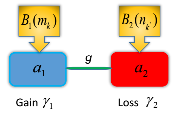
Figure 1: (Color online) The model. Two cavities bearing modes $a_{1}$ and $a_{2}$ coupled through coupling constant $g$ are also interacting with baths $B_{1}$ and $B_{2}$, respectively. The baths cause gain $\gamma_{1}$ and loss $\gamma_{2}$ in the first and second cavity, respectively.

II Model and Solution

In this work, we are interested to study the interplay between PT symmetry and various facets of nonclassicality. To this effect, we consider the system sketched in Fig. 1. Two optical cavities bearing modes $a_{1}$ and $a_{2}$, with corresponding frequencies $\omega_{1}$ and $\omega_{2}$, are connected by coupling constant $g$. The Hamiltonian for this system can be written as

$$H_{S} =\omega_{1}a_{1}^{\dagger}a_{1}+\omega_{2}a_{2}^{\dagger}a_{2}+g(a_{1}^{\dagger}a_{2}+{\rm H.c.}),$$ (1)

where H.c. stands for Hermitian conjugate. Throughout this paper, we are going to work in the natural units ($\hbar=c=1$). To bring the $PT$ symmetric effects, we allow the cavities in the system of interest to interact with the ambient environmental degrees of freedom. We denote the baths (reservoirs) as $B_{1}$ and $B_{2}$ and consider them to be coupled to the cavities bearing modes $a_{1}$ and $a_{2}$, respectively. We further assume that the former cavity has a gain rate $\gamma_{1}$, and the later has a loss rate $\gamma_{2}$. The Hamiltonian pertaining to the baths $(H_{B})$ and the system-bath interaction $(H_{SB})$ are respectively given by

$$H_{B} = \sum_{k}\nu_{k}m_{k}^{\dagger}m_{k}+\sum_{k^{\prime}}\nu_{k^{\prime}}n_{k^{\prime}}^{\dagger}n_{k^{\prime}},$$ (2a)

$$H_{SB} = \left\{\sum_{k}g_{k}m_{k}^{\dagger}a_{1}+\sum_{k^{\prime}}g_{k^{\prime}}n_{k^{\prime}}^{\dagger}a_{2}+{\rm H.c.}\right\}.$$ (2b)

Here, $m_{k}$ and $n_{k}^{\prime}$ are the annihilation operators corresponding to the baths $B_{1}$ and $B_{2}$, respectively, and are coupled to the corresponding cavity modes $a_{1}$ and $a_{2}$ with coupling strengths $g_{k}$ and $g_{k^{\prime}}$. Using Eqs. (1), (2a), and (2b), we obtain the following Langevin equations:

$$\dot{a}_{1}(t) =-i\omega_{1}a_{1}(t)+\gamma_{1}a_{1}(t)+f_{1}(t)-iga_{2}(t),$$ (3a)

$$\dot{a}_{2}(t) =-i\omega_{2}a_{2}(t)-\gamma_{2}a_{2}(t)+f_{2}(t)-iga_{1}(t).$$ (3b)

Here, $f_{1}(t)$ and $f_{2}(t)$ are the noise operators given by $-i\sum_{l}g_{l}b_{l}(0)e^{-i\nu_{l}t}$, where $b_{l}(0)$ denotes the corresponding bath operator. The noise operators satisfy the following properties Agarwal (2013):

$$\langle f_{1}^{\dagger}(t)f_{1}(t^{\prime})\rangle =2\gamma_{1}\delta(t-t^{\prime}),\quad\langle f_{1}(t)f_{1}^{\dagger}(t^{\prime})\rangle=0,$$ (4a)

$$\langle f_{2}(t)f_{2}^{\dagger}(t^{\prime})\rangle =2\gamma_{2}\delta(t-t^{\prime}),\quad\langle f_{2}^{\dagger}(t)f_{2}(t^{\prime})\rangle=0.$$ (4b)

The action of the parity operator $P$ and the time reversal operator $T$ on modes $a_{1}$ and $a_{2}$ can be summarized as

$$P :a_{1}\leftrightarrow-a_{2},\quad a_{1}^{\dagger}\leftrightarrow-a_{2}^{\dagger},$$ (5a)

$$T :a_{1}\leftrightarrow a_{1},\quad a_{1}^{\dagger}\leftrightarrow a_{1}^{\dagger},\quad a_{2}\leftrightarrow a_{2},\quad a_{2}^{\dagger}\leftrightarrow a_{2}^{\dagger}.$$ (5b)

The action of the time reversal operator also flips the sign of the complex number $i$. Thus, the PT invariance of Eqs. (3a) and (3b) demands that

$$\omega_{1}=\omega_{2}=\omega\quad{\textrm{and}}\quad\gamma_{1}=\gamma_{2}=\gamma.$$ (6)

To investigate the PT invariance further, let us redefine the annihilation operators as $\tilde{a}_{1}(t)=e^{-i\omega t}a_{1}(t)$, $\tilde{a}_{2}(t)=e^{-i\omega t}a_{2}(t)$, and the noise operator $F_{i}(t)=e^{-i\omega t}f_{i}(t)$. With this transformation Eqs. (3a) and (3b) become

$$\dot{\tilde{a}}_{1}(t) =\gamma\tilde{a}_{1}(t)+F_{1}(t)-ig\tilde{a}_{2}(t),$$ (7a)

$$\dot{\tilde{a}}_{2}(t) =-\gamma\tilde{a}_{2}(t)+F_{2}(t)-ig\tilde{a}_{1}(t).$$ (7b)

One can write the formal solution of the above equations as follows

$$\begin{pmatrix}\tilde{a}_{1}(t)\\ \tilde{a}_{2}(t)\end{pmatrix}=e^{-i\mathcal{K}t}\begin{pmatrix}\tilde{a}_{1}(0)\\ \tilde{a}_{2}(0)\end{pmatrix}+\int_{0}^{t}ds\,e^{-i\mathcal{K}(t-s)}\begin{pmatrix}F_{1}(s)\\ F_{2}(s)\end{pmatrix}.$$ (8)

Here, $\mathcal{K}$ is identified as the effective Hamiltonian for the system given by

$$\mathcal{K}=\begin{pmatrix}i\gamma&g\\ g&-i\gamma\end{pmatrix}$$ (9)

with eigenvalues

$$\lambda_{\pm}=\begin{cases}\pm\sqrt{g^{2}-\gamma^{2}}&{\rm for~{}}g\geq\gamma,\\ \\ \pm i\sqrt{\gamma^{2}-g^{2}}&{\rm for~{}}g<\gamma.\\ \end{cases}$$ (10)

Apart from the conditions given in Eq. (6), the complete PT invariance demands that the eigenvalues of $\mathcal{K}$ are real, that is $\gamma\leq g$. Naturally, PTSB regime is characterized by $\gamma>g$. In other words, the dominance of the gain/loss over the coupling strength breaks the PT symmetry of the system. The transition from the PTS to PTSB regime is governed by the eigenvalues of the effective Hamiltonian. Figure 2 shows the behavior of the eigenvalues with respect to the coupling strength $g$ and the gain (loss) rate $\gamma$. The two real branches of eigenvalues coalesce at $g=\gamma$ and become complex for $g<\gamma$. These points at which the transition from real to complex spectrum occurs, are known as exceptional points Longhi (2018).

(a)

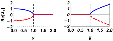
(b)

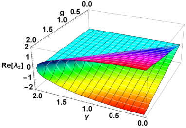
Figure 2: (Color online) The real part of the eigenvalues $\lambda_{\pm}$ is plotted as a function of the coupling strength $g$ and the gain (loss) rate $\gamma$. The points where the two eigenvalues coalesce are called as exceptional points. In (a), the blue (solid) and red (dashed) curves correspond to $\lambda_{+}$ and $\lambda_{-}$, respectively.

We can now rewrite the solution given in Eq. (8) by setting $Q=e^{-i\mathcal{K}t}$. With $\mathcal{K}$ given in Eq. (9), it can be shown that

$$Q=\begin{pmatrix}\cosh(\Omega t)+\frac{\gamma}{\Omega}\sinh(\Omega t)&\frac{-ig}{\Omega}\sinh(\Omega t)\\ \\ \frac{-ig}{\Omega}\sinh(\Omega t)&\cosh(\Omega t)-\frac{\gamma}{\Omega}\sinh(\Omega t)\end{pmatrix}.$$ (11)

Here, $\Omega=\sqrt{\gamma^{2}-g^{2}}$ controls the transition from PTS to PTSB phase. Finally, the solution turns out to be

$$\tilde{a}_{1}(t) =Q_{11}(t)\tilde{a}_{1}(0)+Q_{12}(t)\tilde{a}_{2}(0)$$

$$+\int_{0}^{t}ds\bigg{(}Q_{11}(t-s)F_{1}(s)+Q_{12}(t-s)F_{2}(s)\bigg{)},$$ (12)

$$\tilde{a}_{2}(t) =Q_{21}(t)\tilde{a}_{1}(0)+Q_{22}(t)\tilde{a}_{2}(0)$$

$$+\int_{0}^{t}ds\bigg{(}Q_{21}(t-s)F_{1}(s)+Q_{22}(t-s)F_{2}(s)\bigg{)}.$$ (13)

One can obtain the solution at the exceptional points by taking appropriate limits, specifically considering $\Omega\rightarrow 0$, we can obtain

$$Q|_{\Omega\rightarrow 0}=\begin{pmatrix}1+\gamma t&-igt\\ -igt&1-\gamma t\end{pmatrix}.$$ (14)

Having obtained the solution for the two field modes $\tilde{a}_{1}(t)$ and $\tilde{a}_{2}(t)$, we now proceed to study some properties of the output fields, like average photon numbers with different input states, and also look for the nonclassical features of the fields. Since the phase factor in $\tilde{a}_{k}(t)=e^{-i\omega t}a_{k}(t)$ ($k=1,2$) is not relevant in our study, in what follows, we would drop the tilde.

III Some properties of the output fields

In this section, we analyze some properties associated with the field modes $a_{1}$ (gain) and $a_{2}$ (loss), and their behavior in PTS and PTSB regimes.

Average photon number: We begin this study with the average photon number $n_{a_{i}}=\langle a_{i}^{\dagger}(t)a_{i}(t)\rangle$ corresponding to the mode $a_{i}$ $(i=1,2)$, by choosing different initial states. For example, with the input state as vacuum, one can obtain the following closed form expressions for the average photon number:

$$n_{a_{1}} =\frac{2\gamma^{2}\Omega\cosh(2\Omega t)-(\Omega^{2}+\gamma^{2})\gamma\sinh(2\Omega t)-2\gamma\Omega(\gamma+g^{2}t)}{2\Omega^{3}},$$

$$n_{a_{2}} =\frac{g^{2}\gamma}{2\Omega^{2}}\Big{[}-2t+\frac{\sinh(2\Omega t)}{\Omega}\Big{]}.$$ (15)

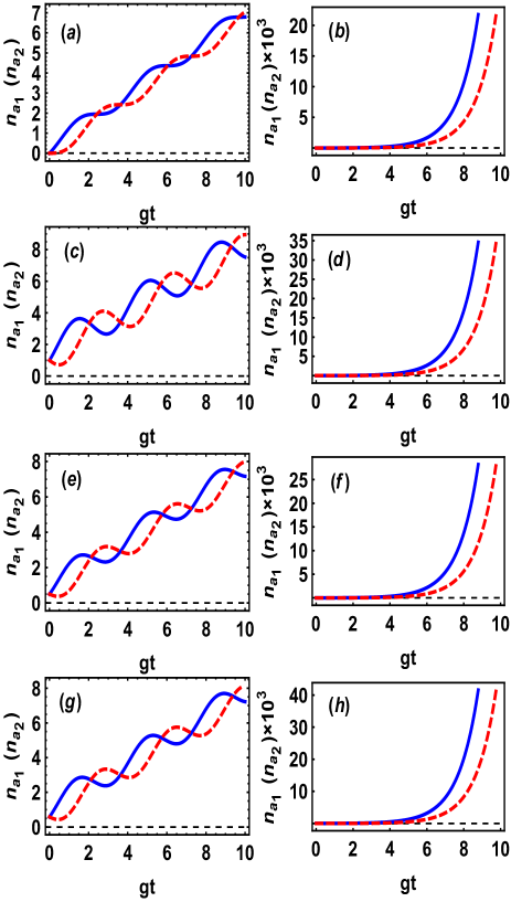
Figure 3: (Color online) Average photon number $n_{a_{1}}=\langle a_{1}^{\dagger}(t)a_{1}(t)\rangle$ (solid blue curve) and $n_{a_{2}}=\langle a_{2}^{\dagger}(t)a_{2}(t)\rangle$ (dashed red curve) with respect to the dimensionless parameter $gt$ for PTS (left panel) and PTSB (right panel) cases. The value of $\gamma$ is $0.5g$ and $1.1g$ corresponding to the PTS and PTSB regimes, respectively. The input states are: (a)-(b) Vacuum state $\ket{00}$; (c)-(d) Coherent state $\ket{\alpha_{1}\alpha_{2}}$, with $\alpha_{k}=r_{k}e^{i\theta_{k}}$ for $k=1,2$ and coherent state parameters $r_{1}=r_{2}=1$, $\theta_{1}=\theta_{2}=\pi/4$; (e)-(f) NOON state $(\ket{10}+\ket{01})/\sqrt{2}$; (g)-(h) Thermal state $\rho_{0}=(1-e^{\beta})^{2}\exp[-\beta(a_{1}^{\dagger}a_{1}+a_{2}^{\dagger}a_{2})]$ with $\beta=\hbar\omega/kT$. Here, we have chosen $\beta=1$.

Similarly, we have considered different initial states, such as coherent state $\ket{\alpha_{1},\alpha_{2}}$, NOON state $(\ket{1,0}+\ket{0,1})/\sqrt{2}$, and thermal state $\rho_{0}=(1-e^{\beta})^{2}\exp[-\beta(a_{1}^{\dagger}a_{1}+a_{2}^{\dagger}a_{2})]$ (see Appendix A), to compute the average photon numbers in the two cavities. The average photon number in each case is plotted in Fig. 3. The parameters $\gamma$ (gain/loss rate) and $g$ (coupling strength) are chosen such that the system is either in PTS or PTSB regime. In the PTS regime, the average photon number for the gain and loss modes is observed to grow together, waning the distinction between gain and loss cavities. In PTSB regime, however, the average photon number in the gain cavity grows faster as compared to the average photon number in the lossy cavity. This is due to the fact that in the PTSB phase, the gain/loss dominates the coupling strength between the two cavities. The oscillatory behavior of the curves in PTS case can be attributed to the fact that the elements of the $Q$ matrix change from hyperbolic to sinusoidal function as one goes from PTSB to PTS regime. The rapid increase in the photon number as a spontaneous photon generation process in the context of PT symmetry was also reported in Agarwal and Qu (2012) in a system of two coupled waveguides. In all these cases, in PTS regime, one can clearly see initial decay in the average photon number in the lossy cavity, which is compensated later by its interaction with the gain medium. In the set of possible input states, we have considered vacuum (shown to play an important role in PTS property Agarwal and Qu (2012)), a quantum state with positive (coherent state) and negative (NOON state) Glauber-Sudarshan $P$ function, and a mixed (thermal) state having positive $P$ function. Average photon numbers of two cavities does not give any signature of quantumness. Therefore, in what follows, we investigate the QZE and QAZE and some nonclassical features, like intermodal antibunching and squeezing, in the field modes, which will use the number operators calculated so far.

Quantum Zeno and anti-Zeno effects: A more general definition of QZE involves the dynamics for which the interaction part may be defined as a ‘continuous gaze’ on the system under consideration (see Facchi and Pascazio (2001) for a review). This interaction may be a measurement operator to explain QZE as introduced in Misra and Sudarshan (1977). In the present case, the two cavity model (in Fig. 1) can be considered as a system-probe configuration, where one of the cavities (considered system) is under a constant influence of the other cavity (probe). The occurrence of QZE and QAZE in the system-probe setting can be studied by defining Zeno parameter, introduced in Thapliyal and Pathak (2015); Thapliyal et al. (2016),

$$\zeta_{a_{i}}(t) =\frac{n_{a_{i}}-n_{a_{i}}|_{g=0}}{\displaystyle\prod_{i=1,2}n_{a_{i}}},$$ (16)

with $n_{a_{i}}=\langle a_{i}^{\dagger}(t)a_{i}(t)\rangle$. Here, we have normalized the Zeno parameter by dividing by the product of the average number of photons of the two modes. A positive (negative) value of the Zeno parameter $\zeta_{a_{i}}$ implies an increase (decrease) in the average photon numbers corresponding to the mode $a_{i}$ as a consequence of the coupling ($g$) with the probe field. The scenarios $\zeta_{a_{i}}(t)<0$ and $\zeta_{a_{i}}(t)>0$ are respectively known as QZE and QAZE.

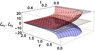
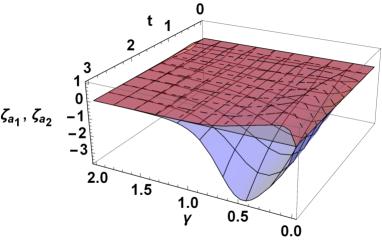
(a) (b) (c)

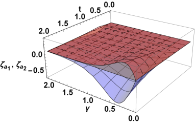
Figure 4: (Color online) Zeno parameter as defined in Eq. (16), $\zeta_{a_{1}}$ (blue surface) and $\zeta_{a_{2}}$ (red surface) with input state as vacuum (a), NOON state $(\ket{10}+\ket{01})/\sqrt{2}$ (b), and thermal state (c). In all the cases, the lossy mode ($a_{2}$) shows the QAZE while the gain mode ($a_{1}$) shows the QZE. Here, we have chosen coupling strength $g=1$, so that $\gamma<1$ and $\gamma>1$ correspond to PTS and PTSB regimes, respectively.

Figure 4 depicts the Zeno parameter with different initial states, viz., vacuum state (a), NOON state $(\ket{10}+\ket{01})/\sqrt{2}$ (b), and thermal state (c). In all the cases, mode $a_{2}$ (red surface) shows the QAZE effect while QZE is displayed by mode $a_{1}$ (blue surface). This nature is observed due to the fact that the number of photons generated under an independent evolution of the gain cavity is suppressed (which is described as QZE) due to its interaction with the lossy cavity. In contrast, an increase in the number of photons (which is described as QAZE) in the lossy cavity is the outcome of its interaction with the gain cavity. This increase/decrease in the number of photons also depends upon the values of parameters deciding PT symmetry property of the system.

(a)
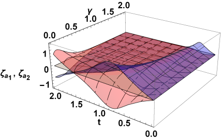
(b)

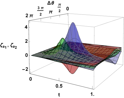
Figure 5: (Color online) Zeno parameter as defined in Eq. (16) with input state as coherent state $\ket{r_{1}e^{i\theta_{1}},r_{2}e^{i\theta_{2}}}$ for $r_{1}=r_{2}=1$. In (a), $\theta_{1}=\pi$, $\theta_{2}=-\pi/4$. The blue and red surfaces correspond to $\zeta_{a_{1}}$ and $\zeta_{a_{2}}$, respectively. Here, the coupling strength between the cavities $g=1$. (b) Variation with respect to the relative phase parameter $\Delta\theta=\theta_{1}-\theta_{2}$. The color scheme is as follows: blue for $\zeta_{a_{1}}$, red for $\zeta_{a_{2}}$ with $\gamma=0.5g$, that is, PTS regime; green for $\zeta_{a_{1}}$ and gray for $\zeta_{a_{2}}$ with $\gamma=1.5g$, PTSB regime. The parameter $\Delta\theta$ decides which of the two modes ($a_{1}$ or $a_{2}$) would show the QZE/QAZE. The maxima and minima in the plot occur at $\Delta\theta=\pi/2,3\pi/2$.

We separately discuss the case when both the cavity fields are initially in the coherent states as in this case, the transition between the QZE and QAZE can be controlled by the parameters of the input fields. Specifically, Fig. 5 depicts the Zeno parameter corresponding to modes $a_{1}$ and $a_{2}$ with input state as the coherent state $\ket{\alpha_{1}\alpha_{2}}$, such that $\alpha_{k}=r_{k}e^{i\theta_{k}}$ with $k=1,2$. Figure 5 (a) shows the variation of the Zeno parameters with respect to the gain/loss rate $\gamma$ and time $t$. In PTS regime ($\gamma<g$), the QZE and QAZE are more prominent as compared to PTSB regime ($\gamma>g$). The observed behavior can be attributed to the fact that in the PTS phase, the coupling is dominant and has pronounced effect, i.e., losses in cavity mode $a_{2}$ are supplemented by the gain cavity due to strong coupling between them. This causes large variation in the Zeno parameter in PTS phase when compared with the PTSB phase. In Fig. 5 (b), the Zeno parameter is shown as a function of the relative phase (difference of the phases corresponding to the coherent states of the two modes) $\Delta\theta=\theta_{1}-\theta_{2}$ and time $t$. It is clear that the presence of QZE or QAZE in modes $a_{1}$ and $a_{2}$ depends on the value of $\Delta\theta$. In this case, for $\Delta\theta>\pi$, the mode $a_{1}$ dominantly shows QAZE, while for $\Delta\theta<\pi$ it shows QZE. Therefore, a transition between QZE and QAZE can be controlled by the relative phase of the input coherent states, while variation in the amount of the Zeno parameter also depends upon whether the system is in the PTS/PTSB phase.

(a)
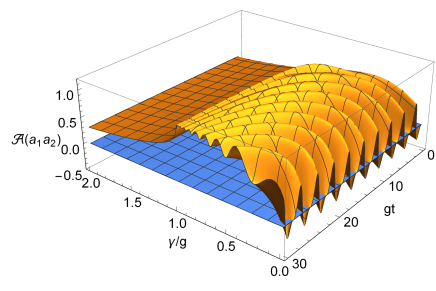
(b)

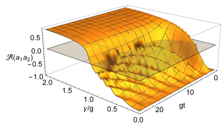
Figure 6: (Color online) Intermodal antibunching with input state as coherent state $\ket{\alpha_{1},\alpha_{2}}$ (a) and NOON state $(\ket{10}+\ket{01})/\sqrt{2}$ (b). In the former $\alpha_{1}=r_{1}e^{i\theta_{1}}$ and $\alpha_{2}=r_{2}e^{i\theta_{2}}$ with $r_{1}=1$, $r_{2}=2$, $\theta_{1}=\theta_{2}=\pi/2$. The nonclassical behavior corresponds to $\mathpzc{A}(a_{1}a_{2})<0$. The behavior in PTS regime ($\gamma<g$) is very different from the PTSB regime ($\gamma>g$).

Intermodal antibunching: For the field modes $a_{1}$ and $a_{2}$, the condition for intermodal antibunching is given as follows

$$\mathpzc{A}(a_{1}a_{2})=\langle a^{\dagger}_{1}a_{2}^{\dagger}a_{1}a_{2}\rangle-\langle a_{1}^{\dagger}a_{1}\rangle\langle a_{2}^{\dagger}a_{2}\rangle<0.$$ (17)

The first term in the right-hand side corresponds to the simultaneous detection in the outputs of two cavities, while the second term represents the product of individual detections in the outputs. In order to compute the first expectation value, we make use of the following decoupling relation (Naikoo et al. (2018) and references therein)

$$\langle ABCD\rangle \approx\langle AB\rangle\langle CD\rangle+\langle AD\rangle\langle BC\rangle+\langle AC\rangle\langle BD\rangle$$

$$-2\langle A\rangle\langle B\rangle\langle C\rangle\langle D\rangle.$$ (18)

Thus, we obtain the average value of the witness of intermodal antibunching $\mathpzc{A}(a_{1}a_{2})$ for different initial states, which detects the presense of nonclassicality for the negative values of the witness $\mathpzc{A}(a_{1}a_{2})$. Figure 6 depicts the variation of the intermodal antibunching witness $\mathpzc{A}(a_{1}a_{2})$ with input state as (a) coherent state and (b) NOON state. The nonclassical features are observed in both the cases as depicted by the negative values of the witness. Further, it is clear that the behavior in PTS and PTSB regimes is remarkably different, revealing that PTS phase favors nonclassicality compared to PTSB phase.

(a)
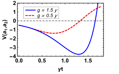
(b)

Figure 7: (Color online) Sum squeezing parameter $V(a_{1},a_{2})$ (a) and difference squeezing parameter $W(a_{1},a_{2})$ (b), as defined in Eqs. (20) and (21), plotted against dimensionless parameter $\gamma t$ with vacuum as the initial state. A state is sum (difference) squeezed if $V(a_{1},a_{2})<0$ $(W(a_{1},a_{2})<0)$. Here, we used $\phi=\pi/4$.

Sum squeezing criterion: Hillery’s sum squeezing criterion Hillery (1989) is defined in terms of a generalized two mode quadrature operator of the form

$$V_{\phi}=\frac{e^{-i\phi}a_{1}a_{2}+e^{i\phi}a_{1}^{\dagger}a_{2}^{\dagger}}{2},$$ (19)

in analogy of the single mode quadrature where $\phi$ is the phase angle of the coherent field used in the homodyne measurement. A state is said to be sum squeezed along phase angle $\phi$, if

$$V(a_{1},a_{2})=\langle(\Delta V_{\phi})^{2}\rangle-\frac{\langle a_{1}^{\dagger}a_{1}\rangle+\langle a_{2}^{\dagger}a_{2}\rangle+1}{4}<0$$ (20)

with $\langle(\Delta V_{\phi})^{2}\rangle=\langle V_{\phi}^{2}\rangle-\langle V_{\phi}\rangle^{2}$.

Difference squeezing criterion: A state is said to be difference squeezed if

$$W(a_{1},a_{2})=\langle(\Delta W_{\phi})^{2}\rangle-\frac{|\langle a_{1}^{\dagger}a_{1}\rangle-\langle a_{2}^{\dagger}a_{2}\rangle|}{4}<0.$$ (21)

The collective operator $W_{\phi}=\frac{1}{2}(e^{i\phi}a_{1}a_{2}^{\dagger}+e^{-i\phi}a_{1}^{\dagger}a_{2})$ and variance $\langle(\Delta W_{\phi})^{2}\rangle=\langle W_{\phi}^{2}\rangle-\langle W_{\phi}\rangle^{2}$.

We have chosen to study the sum and difference squeezing here as these two-mode nonclassical features use the average photon numbers we have studied in the beginning of this section. Figure 7 depicts the variation of the sum and difference squeezing parameters $V(a_{1},a_{2})$ and $W(a_{1},a_{2})$, respectively. The negative values of the parameters $V(a_{1},a_{2})$/$W(a_{1},a_{2})$,for any $\phi$ confirm the existence of the sum/difference squeezing. It can be seen that the sum/difference squeezing is enhanced in PTS regime ($g/\gamma>1$) as compared to PTSB regime ($g/\gamma<1$).

IV Conclusion

We considered a two cavity gain-loss system and discussed the conditions necessary for exhibiting PT invariance. This demanded equal gain-loss in the two cavities. Further, complete PT invariance requires the eigenvalues of the effective Hamiltonian to be real. This condition in turn means that the dominance of the gain/loss over the coupling strength $g$ breaks the PT invariance. With this setting, we studied the average photon number with different initial states, viz., vacuum, NOON, coherent, and thermal states. In all the four cases, the average photon number shows a similar behavior for gain and loss modes in PTS regime. In contrast to this, in PTSB regime, the gain mode is found to dominate over the lossy mode, while both show an exponential growth. We further studied some nonclassical features using the average photon numbers for different initial states. Specifically, we have reported the presence of QZE and QAZE in two cavities and nonclassical features, like intermodal antibunching and sum and difference squeezing. These witnesses of nonclassicality as well as the Zeno parameter exhibit suppression in the nonclassical features when one goes from PTS to PTSB regime. In other words, the dominance of the loss/gain over the coupling strength results in depletion of the nonclassical features of the fields. Further, it’s observed that the relative phase of the input coherent fields provides us a control parameter to switch between QZE and QAZE.

The present study is expected to impact deeper understanding of PT symmetry and the role it can play to probe nonclassicality in the physical systems relevant in the field of quantum optics and information processing.

Appendix A:

Average photon number with initial state as a NOON state. For a general NOON state $\frac{\ket{n,0}+\ket{0,n}}{\sqrt{2}}$, the average photon numbers can be shown to be

$$\begin{array}[]{lcl}\langle a_{1}^{\dagger}(t)a_{1}(t)\rangle&=&\frac{1}{2\Omega^{3}}\left\{-2\gamma(\gamma+g^{2}t)\Omega+n\Omega^{3}\cosh^{2}(\Omega t)\right.\\ &+&2\gamma^{2}\Omega\cosh(2\Omega t)+(g^{2}+\gamma^{2})n\Omega\sinh^{2}(\Omega t)\\ &+&\left.(n\Omega^{2}+2\gamma^{2}-g^{2})\gamma\sinh(2\Omega t)\right\},\\ \langle a_{2}^{\dagger}(t)a_{2}(t)\rangle&=&\frac{1}{2\Omega^{3}}\left\{-2g^{2}\gamma\Omega t+n\Omega^{3}\cosh^{2}(\Omega t)\right.\\ &+&n\Omega(g^{2}+\gamma^{2})\sinh^{2}(\Omega t)+\gamma(g^{2}-n\Omega^{2})\\ &\times&\left.\sinh(2\Omega t)\right\}.\end{array}$$ (A.1)

Average photon number with initial state as a coherent state. With a coherent state of the form $\ket{\alpha_{1},\alpha_{2}}$, such that $\alpha_{1}=r_{1}e^{i\theta_{1}}$ and $\alpha_{2}=r_{2}e^{i\theta_{2}}$, we have the following expression for the average photon numbers:

$$\begin{array}[]{lcl}\langle a^{\dagger}_{1}(t)a_{1}(t)\rangle&=&\frac{1}{2\Omega^{3}}\Bigg{[}\gamma(-g^{2}+2\gamma^{2})\sinh(2\Omega t)\\ &-&2\Omega\gamma(\gamma+g^{2}t)+2\Omega r_{1}^{2}\Omega^{2}\cosh^{2}(\Omega t)\\ &+&2\Omega\gamma^{2}\cosh(2\Omega t)+2\Omega\sinh^{2}(\Omega t)\\ &\times&\bigg{(}\gamma^{2}r_{1}^{2}+g^{2}r_{2}^{2}+2g\gamma r_{1}r_{2}\sin(\Delta\theta)\bigg{)}\\ &+&2\Omega r_{1}\bigg{(}\gamma r_{1}+gr_{2}\sin(\Delta\theta)\bigg{)}\sinh(2\Omega t)\Bigg{]},\\ \langle a^{\dagger}_{2}(t)a_{2}(t)\rangle&=&r_{2}^{2}\cosh^{2}(\Omega t)-\frac{r_{2}\bigg{(}\gamma r_{2}+gr_{1}\sin(\Delta\theta)\bigg{)}\sinh(2\Omega t)}{\Omega}\\ &+&\frac{2\Omega\bigg{(}g^{2}r_{1}^{2}+\gamma^{2}r_{2}^{2}+2g\gamma r_{1}r_{2}\sin(\Delta\theta)\bigg{)}\sinh^{2}(\Omega t)}{2\Omega^{3}}\\ &+&\frac{g^{2}\gamma(-2\Omega t+\sinh(2\Omega t))}{2\Omega^{3}}.\end{array}$$ (A.2)

Average photon number with initial state as a thermal state. The two mode isotropic thermal state can be represented by the normalized density matrix

$$\rho_{0}(\beta) =(1-e^{\beta})^{2}\exp[-\beta(a_{1}^{\dagger}a_{1}+a_{2}^{\dagger}a_{2})],$$

$$=(1-e^{\beta})^{2}\sum_{n_{1},n_{2}=0}^{\infty}\exp(-\beta(n_{1}+n_{2}))|n_{1},n_{2}\rangle\langle n_{1},n_{2}|.$$ (A.3)

Here $\beta=\hbar\omega/k_{B}T$ and we have used the natural units $\hbar=k_{B}=1$. The average photon number in this case is given by

$$\begin{array}[]{lcl}\langle a^{\dagger}_{1}(t)a_{1}(t)\rangle&=&\frac{g^{2}\sinh^{2}(\Omega t)}{\Omega^{2}}(1-e^{\beta})^{2}\sum_{n_{1},n_{2}}e^{-\beta(n_{1}+n_{2})}n_{2}\\ &+&\left\{\cosh(\Omega t)+\frac{\gamma}{\Omega}\sinh(\Omega t)\right\}^{2}(1-e^{\beta})^{2}\\ &\times&\sum_{n_{1},n_{2}}e^{-\beta(n_{1}+n_{2})}n_{1}-\frac{\gamma(g^{2}-2\gamma^{2})\sinh(2\Omega t)}{2\Omega^{3}}\\ &-&\frac{\gamma\left\{2(\gamma+g^{2}t)\Omega-2\gamma\Omega\cosh(2\Omega t)\right\}}{2\Omega^{3}}\\ \langle a^{\dagger}_{2}(t)a_{2}(t)\rangle&=&\frac{g^{2}\sinh^{2}(\Omega t)}{\Omega^{2}}(1-e^{\beta})^{2}\sum_{n_{1},n_{2}}e^{-\beta(n_{1}+n_{2})}n_{2}\\ &+&\left\{\cosh(\Omega t)+\frac{\gamma}{\Omega}\sinh(\Omega t)\right\}^{2}\\ &+&\frac{g^{2}\gamma}{2\Omega^{3}}(-2\Omega t+\sinh(2\Omega t)).\end{array}$$ (A.4)

References

- Misra and Sudarshan (1977) B. Misra and E. C. G. Sudarshan, Journal of Mathematical Physics 18, 756 (1977).
- Barenco et al. (1997) A. Barenco, A. Berthiaume, D. Deutsch, A. Ekert, R. Jozsa, and C. Macchiavello, SIAM Journal on Computing 26, 1541 (1997).
- Beige et al. (2000) A. Beige, D. Braun, B. Tregenna, and P. L. Knight, Physical Review Letters 85, 1762 (2000).
- Search and Berman (2000) C. Search and P. Berman, Physical Review Letters 85, 2272 (2000).
- Zhou et al. (2009) L. Zhou, S. Yang, Y.-x. Liu, C. Sun, and F. Nori, Physical Review A 80, 062109 (2009).
- Maniscalco et al. (2008) S. Maniscalco, F. Francica, R. L. Zaffino, N. L. Gullo, and F. Plastina, Physical review letters 100, 090503 (2008).
- Wang et al. (2008) X.-B. Wang, J. You, and F. Nori, Physical Review A 77, 062339 (2008).
- Erez et al. (2008) N. Erez, G. Gordon, M. Nest, and G. Kurizki, Nature 452, 724 (2008).
- Wüster (2017) S. Wüster, Physical review letters 119, 013001 (2017).
- Cao et al. (2017) Y. Cao, Y.-H. Li, Z. Cao, J. Yin, Y.-A. Chen, H.-L. Yin, T.-Y. Chen, X. Ma, C.-Z. Peng, and J.-W. Pan, Proceedings of the National Academy of Sciences , 201614560 (2017).
- Itano et al. (1990) W. M. Itano, D. J. Heinzen, J. Bollinger, and D. Wineland, Physical Review A 41, 2295 (1990).
- Fischer et al. (2001) M. Fischer, B. Gutiérrez-Medina, and M. Raizen, Physical review letters 87, 040402 (2001).
- Barone et al. (2004) A. Barone, G. Kurizki, and A. Kofman, Physical review letters 92, 200403 (2004).
- Harrington et al. (2017) P. Harrington, J. Monroe, and K. Murch, Physical review letters 118, 240401 (2017).
- Kakuyanagi et al. (2015) K. Kakuyanagi, T. Baba, Y. Matsuzaki, H. Nakano, S. Saito, and K. Semba, New Journal of Physics 17, 063035 (2015).
- Streed et al. (2006) E. W. Streed, J. Mun, M. Boyd, G. K. Campbell, P. Medley, W. Ketterle, and D. E. Pritchard, Physical review letters 97, 260402 (2006).
- Chen et al. (2010) P.-W. Chen, D.-B. Tsai, and P. Bennett, Physical Review B 81, 115307 (2010).
- Helmer et al. (2009) F. Helmer, M. Mariantoni, E. Solano, and F. Marquardt, Physical Review A 79, 052115 (2009).
- Wolters et al. (2013) J. Wolters, M. Strauß, R. S. Schoenfeld, and O. Benson, Physical Review A 88, 020101 (2013).
- Zheng et al. (2013) W. Zheng, D. Xu, X. Peng, X. Zhou, J. Du, and C. Sun, Physical Review A 87, 032112 (2013).
- Kalb et al. (2016) N. Kalb, J. Cramer, D. J. Twitchen, M. Markham, R. Hanson, and T. H. Taminiau, Nature communications 7, 13111 (2016).
- Segal and Reichman (2007) D. Segal and D. R. Reichman, Physical Review A 76, 012109 (2007).
- Chaudhry (2016) A. Z. Chaudhry, Scientific Reports 6, 29497 (2016).
- Eleuch and Rotter (2017) H. Eleuch and I. Rotter, Physical Review E 95, 062109 (2017).
- Zhou et al. (2017) Z. Zhou, Z. Lü, H. Zheng, and H.-S. Goan, Physical Review A 96, 032101 (2017).
- Chaudhry and Gong (2014) A. Z. Chaudhry and J. Gong, Physical Review A 90, 012101 (2014).
- Zhang and Fan (2015) Y.-R. Zhang and H. Fan, Scientific Reports 5, 11509 (2015).
- Maniscalco et al. (2006) S. Maniscalco, J. Piilo, and K.-A. Suominen, Physical review letters 97, 130402 (2006).
- Zhang et al. (2018) J.-M. Zhang, J. Jing, L.-G. Wang, and S.-Y. Zhu, Phys. Rev. A 98, 012135 (2018).
- Eisert et al. (1999) J. Eisert, M. Wilkens, and M. Lewenstein, Phys. Rev. Lett. 83, 3077 (1999).
- Amengual et al. (2004) P. Amengual, A. Allison, R. Toral, and D. Abbott, in Proc. R. Soc. Lond. A, Vol. 460 (The Royal Society, 2004) pp. 2269–2284.
- MEYER and BLUMER (2002) D. A. MEYER and H. BLUMER, Fluctuation and Noise Letters 2, L257 (2002).
- Chandrashekar and Banerjee (2011) C. Chandrashekar and S. Banerjee, Physics Letters A 375, 1553 (2011).
- Pathak and Ghatak (2018) A. Pathak and A. Ghatak, Journal of Electromagnetic Waves and Applications 32, 229 (2018).
- Glauber (1963) R. J. Glauber, Physical Review 131, 2766 (1963).
- Sudarshan (1963) E. C. G. Sudarshan, Physical Review Letters 10, 277 (1963).
- Agarwal (2013) G. S. Agarwal, Quantum Optics (Cambridge University Press, Cambridge, 2013).
- Dowling and Milburn (2003) J. P. Dowling and G. J. Milburn, Philosophical Transactions of the Royal Society of London A: Mathematical, Physical and Engineering Sciences 361, 1655 (2003).
- Browne et al. (2017) D. Browne, S. Bose, F. Mintert, and M. Kim, Progress in Quantum Electronics 54, 2 (2017).
- Horodecki et al. (2009) R. Horodecki, P. Horodecki, M. Horodecki, and K. Horodecki, Reviews of modern physics 81, 865 (2009).
- Cavalcanti and Skrzypczyk (2016) D. Cavalcanti and P. Skrzypczyk, Reports on Progress in Physics 80, 024001 (2016).
- Brunner et al. (2014) N. Brunner, D. Cavalcanti, S. Pironio, V. Scarani, and S. Wehner, Reviews of Modern Physics 86, 419 (2014).
- Gisin et al. (2002) N. Gisin, G. Ribordy, W. Tittel, and H. Zbinden, Reviews of modern physics 74, 145 (2002).
- Shenoy-Hejamadi et al. (2017) A. Shenoy-Hejamadi, A. Pathak, and R. Srikanth, Quanta 6, 1–47 (2017).
- Sen et al. (2013) B. Sen, S. K. Giri, S. Mandal, C. R. Ooi, and A. Pathak, Phys. Rev. A 87, 022325 (2013).
- Alam et al. (2017) N. Alam, K. Thapliyal, A. Pathak, B. Sen, A. Verma, and S. Mandal, arXiv:1708.03967 (2017).
- Naikoo et al. (2018) J. Naikoo, K. Thapliyal, A. Pathak, and S. Banerjee, Phys. Rev. A 97, 063840 (2018).
- Thapliyal et al. (2014a) K. Thapliyal, A. Pathak, B. Sen, and J. Peřina, Phys. Rev. A 90, 013808 (2014a).
- Thapliyal et al. (2014b) K. Thapliyal, A. Pathak, B. Sen, and J. Peřina, Phys. Lett. A 378, 3431 (2014b).
- Giri et al. (2014) S. K. Giri, B. Sen, C. R. Ooi, and A. Pathak, Phys. Rev. A 89, 033628 (2014).
- Giri et al. (2017) S. K. Giri, K. Thapliyal, B. Sen, and A. Pathak, Physica A 466, 140 (2017).
- Bose et al. (1997) S. Bose, K. Jacobs, and P. Knight, Phys. Rev. A 56, 4175 (1997).
- Baghshahi et al. (2015) H. Baghshahi, M. K. Tavassoly, and S. J. Akhtarshenas, Quantum Information Processing 14, 1279 (2015).
- Majumdar et al. (2012) A. Majumdar, M. Bajcsy, and J. Vučković, Phys. Rev. A 85, 041801 (2012).
- Thapliyal et al. (2015) K. Thapliyal, S. Banerjee, A. Pathak, S. Omkar, and V. Ravishankar, Annl. Phys. 362, 261 (2015).
- Chakrabarty et al. (2010) I. Chakrabarty, S. Banerjee, and N. Siddharth, Quantum Information and Computation 11 (2010).
- Thapliyal et al. (2017) K. Thapliyal, N. L. Samantray, J. Banerji, and A. Pathak, Physics Letters A 381, 3178 (2017).
- Malpani et al. (2018) P. Malpani, N. Alam, K. Thapliyal, A. Pathak, V. Narayanan, and S. Banerjee, arXiv preprint arXiv:1808.01458 (2018).
- Bender and Boettcher (1998) C. M. Bender and S. Boettcher, Physical Review Letters 80, 5243 (1998).
- Bender (2007) C. M. Bender, Reps. Prog. Phys. 70, 947 (2007).
- Makris et al. (2008) K. G. Makris, R. El-Ganainy, D. N. Christodoulides, and Z. H. Musslimani, Phys. Rev. Lett. 100, 103904 (2008).
- Klaiman et al. (2008) S. Klaiman, U. Günther, and N. Moiseyev, Phys. Rev. Lett. 101, 080402 (2008).
- West et al. (2010) C. T. West, T. Kottos, and T. c. v. Prosen, Phys. Rev. Lett. 104, 054102 (2010).
- Guo et al. (2009) A. Guo, G. J. Salamo, D. Duchesne, R. Morandotti, M. Volatier-Ravat, V. Aimez, G. A. Siviloglou, and D. N. Christodoulides, Phys. Rev. Lett. 103, 093902 (2009).
- Rüter et al. (2010) C. E. Rüter, K. G. Makris, R. El-Ganainy, D. N. Christodoulides, M. Segev, and D. Kip, Nat. Phys. 6 (2010).
- Chong et al. (2011) Y. D. Chong, L. Ge, and A. D. Stone, Phys. Rev. Lett. 106, 093902 (2011).
- Regensburger et al. (2012) A. Regensburger, C. Bersch, M. A. Miri, G. Onishchukov, D. N. Christodoulides, and U. Peschel, Nature (London) 488 (2012).
- Peng et al. (2014) B. Peng, S. K. Özdemir, F. Lei, F. Monifi, M. Gianfreda, G. L. Long, S. Fan, F. Nori, C. M. Bender, and L. Yang, Nature Physics 10, 394 EP (2014), article.
- Li and Xie (2014) X. Li and X.-T. Xie, Phys. Rev. A 90, 033804 (2014).
- Liu et al. (2017) Y.-L. Liu, R. Wu, J. Zhang, Ş. K. Özdemir, L. Yang, F. Nori, and Y.-x. Liu, Physical Review A 95, 013843 (2017).
- Mostafazadeh (2003) A. Mostafazadeh, Journal of Physics A: Mathematical and General 36, 7081 (2003).
- Jing et al. (2014) H. Jing, S. K. Özdemir, X.-Y. Lü, J. Zhang, L. Yang, and F. Nori, Phys. Rev. Lett. 113, 053604 (2014).
- Lü et al. (2015) X.-Y. Lü, H. Jing, J.-Y. Ma, and Y. Wu, Phys. Rev. Lett. 114, 253601 (2015).
- Liu and Liu (2016) Y.-L. Liu and Y.-x. Liu, arXiv:1609.02722 (2016).
- Liu et al. (2016) Z.-P. Liu, J. Zhang, Ş. K. Özdemir, B. Peng, H. Jing, X.-Y. Lü, C.-W. Li, L. Yang, F. Nori, and Y.-x. Liu, Physical review letters 117, 110802 (2016).
- Li et al. (2016) W. Li, Y. Jiang, C. Li, and H. Song, Scientific Reports 6, 31095 (2016).
- Zhang et al. (2017a) X. Y. Zhang, Y. Q. Guo, P. Pei, and X. X. Yi, Phys. Rev. A 95, 063825 (2017a).
- Agarwal and Qu (2012) G. S. Agarwal and K. Qu, Phys. Rev. A 85, 031802 (2012).
- Zhang et al. (2017b) L. Zhang, G. S. Agarwal, W. P. Schleich, and M. O. Scully, Phys. Rev. A 96, 013827 (2017b).
- Longhi (2018) S. Longhi, Opt. Lett. 43, 5371 (2018).
- Dey et al. (2018) S. Dey, A. Fring, and V. Hussin, in Coherent States and Their Applications (Springer, 2018) pp. 209–242.
- Facchi and Pascazio (2001) P. Facchi and S. Pascazio, in Progress in Optics, Vol. 42, edited by E. Wolf (Elsevier, Amsterdam, 2001) Chap. 3, pp. 147–218.
- Thapliyal and Pathak (2015) K. Thapliyal and A. Pathak, in International Conference on Optics and Photonics 2015, Vol. 9654 (International Society for Optics and Photonics, 2015) p. 96541F.
- Thapliyal et al. (2016) K. Thapliyal, A. Pathak, and J. Peřina, Phys. Rev. A 93, 022107 (2016).
- Hillery (1989) M. Hillery, Phys. Rev. A 40, 3147 (1989).