Quantum remote sensing with asymmetric information gain

Abstract

Typically, the aim of quantum metrology is to sense target fields with high precision utilizing quantum properties. Unlike the typical aim, in this paper, we use quantum properties for adding a new functionality to quantum sensors. More concretely, we propose a delegated quantum sensor (a client-server model) with security inbuilt. Suppose that a client wants to measure some target fields with high precision, but he/she does not have any high-precision sensor. This leads the client to delegate the sensing to a remote server who possesses a high-precision sensor. The client gives the server instructions about how to control the sensor. The server lets the sensor interact with the target fields in accordance with the instructions, and then sends the sensing measurement results to the client. In this case, since the server knows the control process and readout results of the sensor, the information of the target fields is available not only for the client but also for the server. We show that, by using an entanglement between the client and the server, an asymmetric information gain is possible so that only the client can obtain the sufficient information of the target fields. In our scheme, the server generates the entanglement between a solid state system (that can interact with the target fields) and a photon, and sends the photon to the client. On the other hand, the client is required to possess linear optics elements only including wave plates, polarizing beam splitters, and single-photon detectors. Our scheme is feasible with the current technology, and our results pave the way for a novel application of quantum metrology.

I Introduction

Quantum properties such as superposition and entanglement are considered to be useful resources for several information processing tasks Shor (1997); Grover (1997); Harrow et al. (2009); Vandersypen et al. (2001); Bennett and Brassard (1984); Bennett et al. (1992); Gisin et al. (2002); Broadbent et al. (2009); Morimae and Fujii (2013); Takeuchi et al. (2016); Barz et al. (2012); Greganti et al. (2016); Dowling and Milburn (2003); Spiller et al. (2005). For example, a quantum computer efficiently solves some problems that seem to be hard for classical computers Shor (1997); Grover (1997); Harrow et al. (2009); Vandersypen et al. (2001). Quantum cryptography such as quantum key distribution enables two remote parties to communicate in an information-theoretic secure way Bennett and Brassard (1984); Bennett et al. (1992); Gisin et al. (2002). Furthermore, recently, by combining these two concepts, blind quantum computing (BQC) protocols have also been proposed Broadbent et al. (2009); Morimae and Fujii (2013); Takeuchi et al. (2016); Barz et al. (2012); Greganti et al. (2016). BQC enables a client with computationally weak devices to delegate universal quantum computing to a remote server who has a universal quantum computer while the client’s privacy (input, output, and algorithm) is information-theoretically protected.

Quantum metrology is also one of such practical applications of quantum properties Degen et al. (2016); Budker and Romalis (2007); Balasubramanian et al. (2008); Maze et al. (2008); Dolde et al. (2011); Neumann et al. (2013); Wineland et al. (1992); Huelga et al. (1997); Matsuzaki et al. (2011); Chin et al. (2012). By using the superposition property of a qubit Degen et al. (2016), we can improve the sensitivity to measure target fields such as magnetic fields, electric fields, and temperature Budker and Romalis (2007); Balasubramanian et al. (2008); Maze et al. (2008); Dolde et al. (2011); Neumann et al. (2013). When the frequency of the qubit can be shifted by the target fields, a superposition state of the qubit will acquire a phase shift on the non-diagonal terms during the interaction with the target fields. Therefore, the readout of the phase provides us with the information of the target fields. Further, the use of entanglement resources enhances the measurable sensitivity, and an entanglement sensor can beat the standard quantum limit that the sensitivity of any classical sensor is bounded by Wineland et al. (1992); Huelga et al. (1997); Matsuzaki et al. (2011); Chin et al. (2012).

Just as interdisciplinary approaches between quantum computing and quantum cryptography have lead to propose BQC, interdisciplinary approaches between quantum metrology, quantum computing, and quantum cryptography have lead to propose practical quantum sensing protocols Kessler et al. (2014); Dür et al. (2014); Arrad et al. (2014); Herrera-Martí et al. (2015); Unden et al. (2016); Matsuzaki and Benjamin (2017); Higgins et al. (2007); Waldherr et al. (2012); Nakayama et al. (2015); Matsuzaki et al. (2017); Komar et al. (2014); Eldredge et al. (2018); Proctor et al. (2018). For example, while quantum error correction Lidar and Brun (2013) is a concept that has been discussed in the field of quantum computation for the mitigation of errors during the computation, it has been found that the quantum error correction is also useful to improve the sensitivity of quantum sensors Kessler et al. (2014); Dür et al. (2014); Arrad et al. (2014); Herrera-Martí et al. (2015); Unden et al. (2016); Matsuzaki and Benjamin (2017). A phase estimation algorithm Kitaev (1996) for quantum computation has been used to increase the dynamic range of quantum sensors Higgins et al. (2007); Waldherr et al. (2012). Combination of a quantum computer and a quantum sensor provides us with a way to implement a projective measurement of energy on target systems Nakayama et al. (2015); Matsuzaki et al. (2017). Besides them, although a quantum network is an important concept in quantum cryptography Sasaki et al. (2011); Wang et al. (2013), a network of quantum sensors is also becoming an attractive topic in quantum metrology Komar et al. (2014); Eldredge et al. (2018). This is because a quantum sensing network can enhance the estimation precision under certain conditions Proctor et al. (2018). Also, there are researches that combine the quantum cryptography and quantum metrology Giovannetti et al. (2001); Giovannetti et al. (2002a, b); Chiribella et al. (2005, 2007); Huang et al. (2017); Xie et al. (2018). In the setup of these researches, a few nodes exist, and there are noisy channels between them. The aim of these researches is to share the sensing results (measured at a node) between the nodes without leaking the information to an eavesdropper that has an access to the channels.

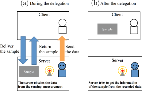
Figure 1: A schematic diagram to illustrate client-server based quantum sensing. We consider the cases during and after the delegation of the sensing. (a) During the delegation, the client sends a sample to the server who holds a high-precision quantum sensor. The client gives the server instructions about how to control the quantum sensor for the measurement of the sample, and the server obeys the instructions. The server sends the measurement results to the client, and the server returns the sample to the client. (b) After the delegation, the server can try to estimate the information of the sample from the classical data remaining in the server’s quantum sensor. Interestingly, our protocol described in this paper prevents the server from obtaining the information of the sample from the remaining data while the client can recover the information of the sample, which we call asymmetric information gain.

In this paper, we also take an interdisciplinary approach to add novel functionality to quantum sensors. Our protocol is based on an idea to combine the BQC and quantum metrology. More concretely, we discuss a situation that a client who does not have any quantum sensor tries to have an access of a remote quantum sensor that belongs to a server at a remote site. This situation is given as Fig. 1. First, the client sends a sample to be measured to the server, and then gives the server instructions about how to use the sensor for the measurement of the sample. Second, according to the instructions, the server lets the sensor interact with the target field (the sample). Finally, the server sends the sensing measurement results and returns the sample to the client. We assume here that the server obeys the client’s instructions during the delegation of quantum sensing. This assumption seems to be reasonable as if the sample is a macroscopic object, it is hard to encrypt the sample. In fact, if we allow the server’s deviation from the instructions during the delegation, the server can easily obtain the information about the sample without being noticed by the client. This is a large difference between the situation of our paper and that of BQC, since the input of BQC is typically an input of a mathematical problem. Even under this assumption, since the classical information about the control process and readout results of the sensor remains at the server’s place after the delegation, the information of the target field should be available not only for the client but also for the server as shown in Fig. 1 (b). This is problematic when the client does not want to reveal the information of the sample.

Then, we will consider the following question: even if the classical information about the control process and readout results of the sensor remain in the server’s quantum sensor after the delegation, can we construct a protocol such that the client obtains the sufficient information of the target field while the server cannot do it? We will show that such an asymmetric information gain between the client and server from the quantum sensor is possible by using entanglement and a reasonably realistic experimental setup.

Standard quantum teleportation Bennett et al. (1993); Bouwmeester et al. (1997); Furusawa et al. (1998) can be a way to realize the asymmetric information gain, which, however, may have a technical problem in terms of feasibility as we will discuss. A superposition state of a qubit for the sensing can acquire a relative phase due to the target fields, and this state can be teleported to the site of the client by the quantum teleportation if an ideal Bell pair is available between the client’s site and the server’s site. In this case, only the client knows the value of the qubit phase where the information of target fields is encoded. However, in this method, the client needs to keep one half of the Bell pair until the outcome of the Bell measurement is sent from the server. This means that the client should have a quantum memory Julsgaard et al. (2004). Although a long-lived quantum memory is possible in the state of art technology Hedges et al. (2010), it would be more feasible if the asymmetric information gain can be realized with less demanding conditions. Furthermore, since it is difficult to share the ideal Bell pairs, the client has to certify how well the server prepares the Bell pair. Therefore, in this paper, we will propose a more feasible scheme that can estimate the fidelity between an actual state and the ideal Bell pair, and does not require any quantum memory for the client’s site.

We explain the basic ideas of our scheme. As shown in Fig. 2, the standard quantum metrology consists of three steps such as the state preparation (the preparation of $|+\rangle\equiv(|0\rangle+|1\rangle)/\sqrt{2}$), the interaction with target fields, and the readout of the qubit (for details, see Sec. II). In order to propose our remote sensing protocol, we divide the state preparation step into two steps, i.e. the Bell pair generation and the client’s subsequent measurement. First, in the Bell pair generation, the client estimates the fidelity between the actual two-qubit state $\rho$ prepared by the server and the ideal Bell pair. If $\rho$ is close to the ideal Bell pair, the client accepts it. Otherwise, the client rejects. Thanks to this step, we can remove the necessity of the ideal Bell pair from our protocol. Note that in general, errors in a channel between the client and the server vary depending on the time. Therefore, we cannot use the quantum state tomography Smithey et al. (1993); Hradil (1997); Banaszek et al. (1999) and the process tomography Poyatos et al. (1997); Chuang and Nielsen (1997) for our purpose. After the client accepts $\rho$, by measuring one half of $\rho$, the client prepares a single-qubit state at the server’s side. Finally, the server performs the standard quantum metrology using the single-qubit state instead of $|+\rangle$, and sends the measurement result to the client. The key idea of our protocol is that the state of the single qubit is known for the client because the client knows the measurement outcome while the server cannot know the state. This difference results in the asymmetric information gain where the client obtain the sufficient information of the sample while the server does not obtain it. Although some readers may think that the server can also obtain the sufficient information by performing the standard quantum metrology with initial state $|+\rangle$ in parallel, this deviation is prohibited by our assumption mentioned above.

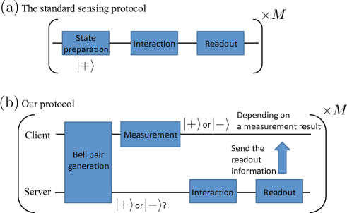
Figure 2: Comparison of the standard sensing protocol with our remote sensing protocol. Here, $|\pm\rangle\equiv(|0\rangle\pm|1\rangle)/\sqrt{2}$ and $M$ is the repetition number. (a) In the standard protocol, there are three steps such as the state preparation, the interaction, and the readout. (b) In our protocol, the state preparation is composed of the Bell pair generation (between the server and the client) and a subsequent measurement by the client, while the interaction and the readout are implemented at the server’s side similar to the standard protocol. Since the server does not know the client’s measurement result, the server cannot know which single-qubit state is prepared at the server’s side before the interaction while the client can know it. This difference realizes the asymmetric information gain.

From an experimental point of view, our protocol would corresponds to a situation that, after the server generates a Bell pair between a solid-state qubit and a flying qubit such as a photon, the photon is sent to the client and is measured by the client immediately after the photon arrives at the client’s side. Therefore, the client does not need any quantum memory, and the only requirement for the client is an ability to measure the flying qubits (photons), which can be implemented by just basic linear optics elements such as a wave plate, a polarizing beam splitter, and single-photon detectors. In general, imperfections of projective measurements on the qubits decrease the sensitivity as a quantum sensor. While there are commercially available single photon detectors, an accurate projective measurement on the solid-state qubit is not a mature technology yet, and not every researcher is capable of implementing precise projective measurements on the solid state qubits. In our quantum remote sensing protocol, even when the client does not have high-precision projective measurement apparatuses of the solid-state qubits, the client can delegate the standard sensing protocol to the server with a technology of accurate projective measurements, and so the client can measure the sample with better sensitivity. To achieve this goal, we use the quantum property such as entanglement.

The rest of this paper is organized as follows: In Secs. II and III, as preliminaries, we review the standard quantum metrology and a random-sampling test, which is a fidelity estimation protocol for Bell pairs. In Sec. IV, by combining the standard quantum metrology and the random-sampling test, we propose the quantum remote sensing protocol. In Sec. IV.1, we give a procedure of our protocol. In Sec. IV.2, we derive the upper bound of the uncertainty obtained by the client. In Sec. IV.3, we derive the lower bound of the uncertainty obtained by the server. In Sec. IV.4, from these bounds of uncertainties, we show that our protocol achieves the asymmetric information gain. In Sec. V, we discuss possible experimental implementations of our protocol. In Sec. VI, we conclude our discussion.

II Quantum metrology

Let us review the standard quantum metrology by using a single-qubit state. A Hamiltonian of the qubit is given as

$$\hat{\mathcal{H}}=\frac{{\color[rgb]{0,0,0}\hbar}\omega}{2}\hat{\sigma}_{z},$$ (1)

where $\omega$ denotes the angular frequency of the qubit. Suppose that we can linearly shift the resonant frequency by external fields such as $\omega\propto B$, where $B$ denotes the amplitude of the target field. By estimating the resonant frequency, we can determine the amplitude of the target field. For such an estimation, a typical Ramsey-type measurement can be used. The procedure is as follows:

1. Prepare an initial state $|+\rangle$.

2. Let the state $|+\rangle$ evolve by the Hamiltonian in Eq. (1) for a time $t$.

3. Measure the state by a projection operator of $\hat{\mathcal{P}}=(\openone+\hat{\sigma}_{y})/2$.

4. Repeat steps 1-3 within a given total time $T$.

The number of repetitions is described by $M=T/(t_{\rm{p}}+t+t_{\rm{r}})$ where $t_{\rm{p}}$ ($t_{\rm{r}}$) denotes the required time for the preparation (readout) of the state. From these repetitions, we obtain $M$ measurement results $\{m_{1},m_{2},\cdots,m_{M}\}$, where $m_{j}\in\{0,1\}$ $(1\leq j\leq M)$. By using the average value $S_{M}=(\sum_{j=1}^{M}m_{j})/M$, we can estimate the target parameter $\omega$. The above procedure is shown by a quantum circuit in Fig. 3.

The uncertainty $\delta\omega$ of the resonant frequency can be calculated as follows: we have the probability $P\equiv{\rm Tr}[\hat{\mathcal{P}}e^{-i\hat{\mathcal{H}}t{\color[rgb]{0,0,0}/\hbar}}|+\rangle\langle+|e^{i\hat{\mathcal{H}}t{\color[rgb]{0,0,0}/\hbar}}]$ of obtaining $m_{j}=1$. From Eq. (1), we obtain $P=(1+\sin\omega t)/2\simeq(1+\omega t)/2$, where we assume $|\omega t|\ll 1$ because we are interested in detecting a small amplitude of the target field. Throughout of this paper, we assume the same condition. From the average value $S_{M}$, one can define an estimated value of $\omega$ such as $\omega^{(\rm{est})}_{M}=(2S_{M}-1)/t$. We have

$$\delta^{2}P = M\langle(S_{M}-P)^{2}\rangle$$

$$\simeq M\frac{t^{2}}{4}\langle(\omega_{M}^{(\rm{est})}-\omega)^{2}\rangle$$

where $\langle\cdot\rangle$ denotes the statistical average and $\delta^{2}P=P(1-P)$ denotes the variance. So we obtain

$$\delta\omega\simeq\frac{1}{t\sqrt{M}}$$

where $\delta\omega\equiv\sqrt{\langle(\omega_{M}^{(\rm{est})}-\omega)^{2}\rangle}$ denotes the uncertainty of the estimation.

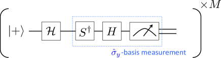
Figure 3: The quantum circuit representation of the standard quantum metrology protocol. Here, $\mathcal{H}$ represents the time evolution by the Hamiltonian in Eq. (1), $S^{\dagger}\equiv|0\rangle\langle 0|-i|1\rangle\langle 1|$, $H$ is the Hadamard gate, and the meter symbol represents the $\hat{\sigma}_{z}$-basis measurement.

III Random-sampling test for Bell pairs

In our quantum remote sensing protocol, it is important to share the Bell pair between the client and the server. However, there are usually many possible error sources in a channel between the client and the server, and they decrease the fidelity with the Bell pair. Since such the infidelity with the Bell pair will affect the performance of our protocol to obtain the asymmetric information gain (as we will describe later), it is important to estimate a lower bound of the fidelity between an actual two-qubit state $\rho$ prepared by the remote server and the ideal Bell pair $|\Phi^{+}\rangle\equiv(|00\rangle+|11\rangle)/\sqrt{2}$. More precisely, in order to derive the uncertainty of the delegated quantum sensing, we have to guarantee that the two-qubit state $\rho$ satisfies $\langle\Phi^{+}|\rho|\Phi^{+}\rangle\geq 1-\epsilon$ with probability at least $1-\delta$ $(0<\epsilon,\delta\leq 1)$. Since errors in the channel may vary depending on the time, we cannot assume any independent and identically distributed (i.i.d.) property. This means that the quantum state tomography Smithey et al. (1993); Hradil (1997); Banaszek et al. (1999) and the process tomography Poyatos et al. (1997); Chuang and Nielsen (1997) are not appropriate for our purpose. In order to estimate the fidelity without assuming any i.i.d. property, we use a destructive random-sampling test Nielsen and Chuang (2000); Takeuchi et al. (2018). For the completeness of the paper, we review the random-sampling test for the Bell pair.

The test runs as follows:

1. A client sets three parameters $\epsilon$, $\delta$, and $\Delta$. Here, $\Delta$ determines the error-robustness of the random-sampling test, and $0\leq\Delta<\epsilon/3$. The client tells these three values to the remote server.

2. The server sends an $8k$-qubit state $\rho_{S}$ to the client, where

   $$k=\left\lceil\cfrac{75}{8(\epsilon-3\Delta)^{2}}\log{\cfrac{2}{\delta}}\right\rceil$$ (2)

   with $\lceil\cdot\rceil$ being the ceiling function. Without loss of generality, we can assume that the state $\rho_{S}$ consists of $4k$ registers, and each register stores two qubits. If the state $\rho_{S}$ is not disturbed by any channel noise, $\rho_{S}=(|\Phi^{+}\rangle\langle\Phi^{+}|)^{\otimes 4k}$. Otherwise, $\rho_{S}$ is arbitrary $8k$-qubit quantum state whose registers may be entangled.

3. The client chooses $k$ registers from $4k$ registers independently and uniformly at random, and then the client measures each of them in the $\hat{\sigma}_{x}\otimes\hat{\sigma}_{x}$ basis, which we call the $X$ test. If two outcomes on two qubits in the same register are the same, we say the register passes the $X$ test. Otherwise, it fails the $X$ test.

4. The client chooses $k$ registers from the remaining $3k$ registers independently and uniformly at random, and then the client measures each of them in the $\hat{\sigma}_{z}\otimes\hat{\sigma_{z}}$ basis, which we call the $Z$ test. If two outcomes on two qubits in the same register are the same, we say the register passes the $Z$ test. Otherwise, it fails the $Z$ test.

5. The client chooses one register, which we call the target register, from the remaining $2k$ registers uniformly at random. Other remaining registers are discarded.

6. The client counts the number $N_{\rm fail}$ of registers that fail the $X$ test or the $Z$ test. If $N_{\rm fail}\leq 2k\Delta$, the client keeps the target register. Otherwise, the client discards it.

Note that in the random-sampling test, we do not assume any i.i.d. property of the $4k$ registers. Therefore, this test works for any channel noise. This test also works for a certain error in the server’s apparatus if it can be treated as a channel noise. This is why we do not have to assume that all of the server’s operations are perfect.

In step 5, $2k-1$ registers are discarded. Although this may seem to be a huge waste, this discarding is necessary to show Theorem 2, which is given later. Fidelity estimation protocols that do not discard any register have already been proposed Hayashi and Morimae (2015); Markham and Krause (2018), but they have no error tolerance, i.e. $\Delta=0$. An effective use of discarded registers has also been discussed in Ref. Takeuchi et al. (2018).

In order to show that the random-sampling test works correctly as a fidelity estimation protocol, we show two properties, so called the completeness and the soundness. Intuitively, if the client can accept the ideal Bell pair $|\Phi^{+}\rangle$ with high probability, we say that the random-sampling test has the completeness. Thanks to the completeness, the client does not mistakenly reject $|\Phi^{+}\rangle$. On the other hand, if the random-sampling test guarantees that an accepted quantum state is close to $|\Phi^{+}\rangle$ with high probability, we say that it has the soundness. Thanks to the soundness, the client does not mistakenly accept a quantum state that is far from $|\Phi^{+}\rangle$. More rigorously, the following two theorems hold:

Theorem 1 (Completeness)

When $\rho_{S}=(|\Phi^{+}\rangle\langle\Phi^{+}|)^{\otimes 4k}$, the client does not discard the target register in step 6 (i.e. the random-sampling test succeeds) with unit probability.

Proof. The Bell pair $|\Phi^{+}\rangle$ is stabilized by $\hat{\sigma}_{x}\otimes\hat{\sigma}_{x}$ and $\hat{\sigma}_{z}\otimes\hat{\sigma}_{z}$. In other words, the Bell pair satisfies

$$\hat{\sigma}_{x}\otimes\hat{\sigma}_{x}|\Phi^{+}\rangle=\hat{\sigma}_{z}\otimes\hat{\sigma}_{z}|\Phi^{+}\rangle=|\Phi^{+}\rangle.$$

Accordingly, $|\Phi^{+}\rangle$ always passes the $X$ test and the $Z$ test. Since the number $N_{\rm fail}$ of registers that fail the $X$ test or the $Z$ test is $0$, the client does not discard the target register in step 6 with unit probability. (Remember that the client does not discard the target register in step 6 when $N_{\rm fail}\leq 2k\Delta$, and $\Delta\geq 0$.) $\blacksquare$

Theorem 2 (Soundness)

In step 5, the state $\rho_{\rm tgt}$ of the target register, which is a single register chosen in step 5, satisfies

$$\langle\Phi^{+}|\rho_{\rm tgt}|\Phi^{+}\rangle\geq 1-\epsilon{\color[rgb]{0,0,0}+3\Delta-\cfrac{3N_{\rm fail}}{2k}}$$ (3)

with probability at least $1-\delta$.

In general, the client cannot determine the value of $N_{\rm fail}$ without performing experiment. However, once $N_{\rm fail}\leq 2k\Delta$ holds, Eq. (3) gives the client the non-trivial lower bound $1-\epsilon$. A proof of Theorem 2 is given in Appendix A.

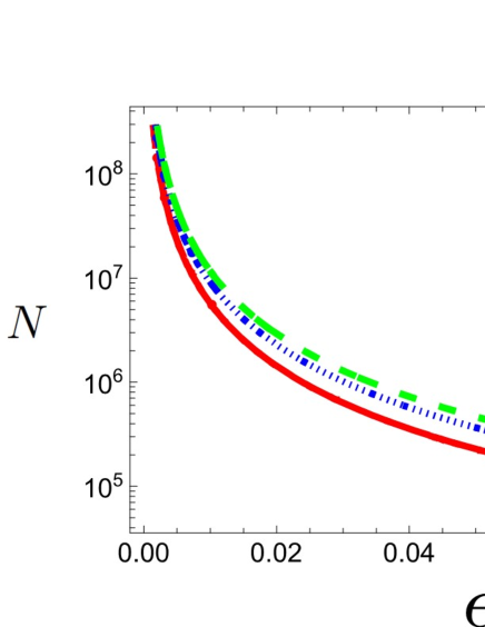
Figure 4: The required number $N=8k$ of qubits as a function of $\epsilon$. Here, $k=\left\lceil 75\log{(2/\delta)}/[8(\epsilon-3\Delta)^{2}]\right\rceil$. The bottom, middle, and top lines show the value of $8k$ for $(\delta,\Delta)=(10^{-3},0)$, $(10^{-5},0)$, and $(10^{-3},\epsilon/10)$, respectively.

Using Eq. (2) and Theorem 2, we can derive how many qubits are necessary to prepare a two-qubit state $\rho_{\rm tgt}$ whose fidelity is at least $1-\epsilon$ with probability $1-\delta$. Note that for simplicity, we here consider the situation where $N_{\rm fail}\leq 2k\Delta$ holds with unit probability. As examples, we explain two cases where this condition is satisfied. First, the ideal (noiseless) channel can satisfy the condition. Second, we can consider a channel noise where the identity operation, the bit-flip operation $(\hat{\sigma}_{x})$, the phase-flip operation $(\hat{\sigma}_{z})$, or the bit- and phase-flip operation $(\hat{\sigma}_{x}\hat{\sigma}_{z})$ is periodically applied. Suppose that Bob sends one half of a single register (two-qubit state) per a certain time $\tau_{\rm{B}}$, and one of three error operations ($\hat{\sigma}_{x}$, $\hat{\sigma}_{z}$, and $\hat{\sigma}_{x}\hat{\sigma}_{z}$) is applied once every $\tau_{\rm{B}}/\Delta$. In this case, $N_{\rm fail}$ is definitely less than or equal to $2k\Delta$. Note again that this situation is just a hypothetical one to simplify the discussion. Theorem 2 also holds for other situations. In Fig. 4, for some specific values of $\delta$ and $\Delta$, we show the $\epsilon$-dependence of the number $8k$ of qubits.

IV Quantum remote sensing

In this section, as a main result, we propose a quantum remote sensing protocol. Simply speaking, our protocol runs as follows: first, the client and the server try to share a Bell pair. In this step, since the Bell pair is disturbed by channel noises, they estimate the fidelity between the actual shared two-qubit state $\rho$ and the ideal Bell pair $|\Phi^{+}\rangle$ using the random-sampling test. Second, if $\rho$ is sufficiently close to $|\Phi^{+}\rangle$, the client measures his/her half of $\rho$ to prepare a single-qubit state at the server’s side. Finally, the server performs the standard quantum metrology protocol using the single-qubit state, and then sends the readout result to the client. Since the server cannot know which state is prepared by the client, our protocol achieves the asymmetric information gain.

IV.1 Protocol

By combining the standard quantum metrology protocol given in Sec. II and the random-sampling test given in Sec. III, we now propose the quantum remote sensing protocol. In order to fit the random-sampling test to our quantum remote sensing protocol, we slightly modify the random-sampling test. In the random-sampling test given in Sec. III, the $8k$-qubit state $\rho_{S}$ is sent simultaneously in step 2. In this case, a quantum memory is needed for the client. In order to remove the necessity of the quantum memory from the client, the server sends each qubit one by one to the client, and the client randomly chooses his/her action from the $X$ test, $Z$ test, discarding, and the $\hat{\sigma}_{x}$-basis measurement on the one half of the target register. The $\hat{\sigma}_{x}$-basis measurement is necessary to prepare a single-qubit state at the server’s side, which is used to perform the standard quantum metrology protocol. Furthermore, we partition the $X$ test and the $Z$ test, which are performed by the client in Sec. III, into the client’s and the server’s measurements.

Our quantum remote sensing protocol runs as follows:

1. The client sets three parameters $\epsilon$, $\delta$, and $\Delta$, where $0\leq\Delta<\epsilon/3$. The client tells these three values to a remote server.

2. The server prepares an $8k$-qubit state $\rho_{S}$, where

   $$k=\left\lceil\cfrac{75}{8(\epsilon-3\Delta)^{2}}\log{\cfrac{2}{\delta}}\right\rceil$$

   with $\lceil\cdot\rceil$ being the ceiling function. The state $\rho_{S}$ consists of $4k$ registers, and each registers store two qubits.

3. The client chooses $k$ registers, which we call the $X$ set, from $4k$ registers independently and uniformly at random. Then, the client tells the server which registers are selected as the $X$ set.

4. The client chooses $k$ registers, which we call the $Z$ set, from the remaining $3k$ registers independently and uniformly at random. Then, the client tells the server which registers are selected as the $Z$ set.

5. The client chooses one register, which we call the target register, from the remaining $2k$ registers independently and uniformly at random. Then, the client tells the server which register is selected as the target register.

6. The server sends one half of each register to the client one by one. (In total, the server sends $4k$ qubits to the client.)

7. The client and the server perform one of following four steps for each register:

   1. If a register is in the $X$ set, the client and the server measure it in the $\hat{\sigma}_{x}^{(C)}\otimes\hat{\sigma}_{x}^{(S)}$ basis, where the superscripts $C$ and $S$ represent an operator applied on the client’s site and the server’s site, respectively. If the client’s and the server’s outcomes are the same, we say the register passes the $X$ test. Otherwise, it fails the $X$ test. Note that they can check whether or not their outcomes are the same by classical communication.

   2. If a register is in the $Z$ set, the client and the server measure it in the $\hat{\sigma}_{z}^{(C)}\otimes\hat{\sigma}_{z}^{(S)}$ basis. If the client’s and the server’s outcomes are the same, we say the register passes the $Z$ test. Otherwise, it fails the $Z$ test.

   3. If a register is the target register, the client measures the one half of the target register in the $\hat{\sigma}_{x}^{(C)}$ basis to prepare a single-qubit state $\rho_{\rm QRS}$ at the server’s site. Let $s\in\{0,1\}$ be the measurement outcome. Then, the server stores $\rho_{\rm QRS}$ in his/her quantum memory.

   4. Otherwise, the client and the server discard the register.

8. The client counts the number $N_{\rm fail}$ of registers that fail the $X$ test or the $Z$ test. If $N_{\rm fail}\leq 2k\Delta$, the random-sampling test succeeds, and the client proceeds to the next step. Otherwise, the test fails, and the client aborts the protocol.

9. The server performs the standard quantum metrology given in Sec. II where the initial state is replaced with the quantum state $\rho_{\rm QRS}$. More specifically, the single-qubit state $\rho_{\rm QRS}$ is evolved by the Hamiltonian in Eq. (1) and then measured in the $\hat{\sigma}_{y}$ basis. The server sends the measurement outcome $o\in\{0,1\}$ to the client.

10. The client calculates $s\oplus o$ and accepts it as the result of the sensing.

11. The client and the server repeat steps 1-10 $M$ times to obtain sufficiently high precision.

We will show that our quantum remote sensing protocol achieves the asymmetric information gain. In other words, the uncertainty of the estimation of the client becomes much smaller than that of the server. Since the small uncertainty implies the success of the metrology, this asymmetric property means that the client can obtain more accurate information of the sensing results than the server. This asymmetry comes from the fact that the measurement outcome $s$ in step 7 (c) is known only for the client. To quantify such the asymmetric information gain between the client and server, we calculate the averaged uncertainty over the outcome $s$ from each point of view. We assume here that each repetition is independent from the others, which means that the probability of the measurement at step 9 in a repetition has no correlation with that in the other repetitions. This assumption is needed to calculate the uncertainty. Also, due to this, we can decrease the uncertainty of the estimation by increasing the repetition number $M$. On the other hand, in the steps from 1 to 10 inside a single repetition, we do not assume any i.i.d. property about the quantum states. These assumptions seem to be reasonable especially when the state preparation time $t_{\rm{p}}$ is much shorter than the interaction time $t$. More concretely, since the $8k$-qubit state $\rho_{S}$ is generated in a short time, $8k$ qubits may be correlated each other. On the other hand, since the interaction time is long, i.e. the time interval between each repetition is long, the $8k$-qubit state $\rho_{S}$ prepared in the $i$th $(1\leq i\leq M-1)$ repetition should not correlate with that prepared in the $(i+1)$th repetition.

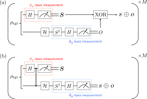
Figure 5: (a) The quantum circuit representation of our delegated metrology where $\rho_{\rm tgt}$ denotes the state of the target register between the server and the client. It is worth mentioning that, by taking a large limit of the number $k$, $\rho_{\rm tgt}$ approaches the ideal Bell pair. (b) The quantum circuit equivalent to the circuit in (a). The vertical line represents the controlled-$\hat{\sigma}_{z}$ gate $|0\rangle\langle 0|\otimes I+|1\rangle\langle 1|\otimes\hat{\sigma}_{z}$. These two circuits output $s\oplus o$ with the same probability.

IV.2 Uncertainty of the client

Let us first calculate the averaged uncertainty of the client. Hereafter, for simplicity, we only consider the situation where $N_{\rm fail}\leq 2k\Delta$ holds with unit probability. To this end, we derive the initial state $\rho_{\rm QRS}$ of the standard quantum metrology protocol. We give a quantum circuit corresponding to our quantum remote sensing protocol in Fig. 5 (a). By transforming the quantum circuit in Fig. 5 (a), we obtain the quantum circuit in Fig. 5 (b). Since these two quantum circuits output $s\oplus o$ with the same probability, the uncertainties calculated from these two quantum circuits are also the same. Let $p_{s}$ and $\rho^{(s)}$ be the probability of the client obtaining the measurement outcome $s$ and the single-qubit state prepared when the measurement outcome is $s$, respectively. In Fig. 5 (b), $\sum_{s=0}^{1}p_{s}\hat{\sigma}_{z}^{s}\rho^{(s)}\hat{\sigma}_{z}^{s}$ is used as the initial state of the standard quantum metrology protocol. Therefore, we can assume that $\rho_{\rm QRS}=\sum_{s=0}^{1}p_{s}\hat{\sigma}_{z}^{s}\rho^{(s)}\hat{\sigma}_{z}^{s}$. Note that the quantum circuit in Fig. 5 (b) does not achieve the asymmetric information gain because the value of $s\oplus o$ is revealed also for the server. However, our present aim is to calculate the uncertainty. Therefore, we can replace the quantum circuit in Fig. 5 (a) with that in Fig. 5 (b).

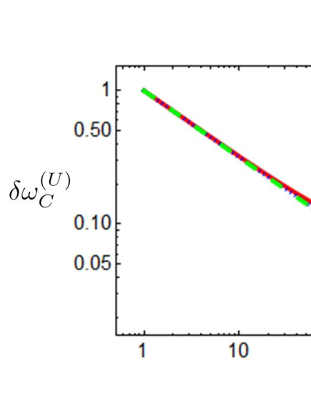
Figure 6: The client’s uncertainty $\delta\omega_{{C}}^{({U})}$against the number $M$ of repetitions where we set $t=1$. Although the horizontal axis represents discrete values, we use continuous lines for plots as guides for the eyes.

From Theorem 2, the target register satisfies $\langle\Phi^{+}|\rho_{\rm tgt}|\Phi^{+}\rangle\geq 1-\epsilon$ with probability at least $1-\delta$. Therefore, for the virtual initial state $\sum_{s=0,1}p_{s}\hat{\sigma}_{z}^{s}\rho^{(s)}\hat{\sigma}_{z}^{s}$, the following corollary holds:

Corollary 1

$\langle+|\sum_{s=0,1}p_{s}\hat{\sigma}_{z}^{s}\rho^{(s)}\hat{\sigma}_{z}^{s}|+\rangle\geq 1-\epsilon$ with a probability at least $1-\delta$.

Proof. We use the monotonicity of the fidelity, i.e. a property that the fidelity is not decreased by any trace-preserving (TP) map. First, we consider the non-demolition $\hat{\sigma}_{x}$-basis measurements on the first qubits of $|\Phi^{+}\rangle$ and $\rho_{\rm tgt}$. Note that these non-demolition measurements are not performed in practice. These are only used to show this corollary. Then, the Hadamard gates are applied on the first qubits. As a result, $|\Phi^{+}\rangle$ and $\rho_{\rm tgt}$ becomes

$$\cfrac{|0+\rangle\langle 0+|+|1-\rangle\langle 1-|}{2}$$ (4)

and

$$p_{0}|0\rangle\langle 0|\otimes\rho^{(0)}+p_{1}|1\rangle\langle 1|\otimes\rho^{(1)},$$ (5)

respectively. Here, $|-\rangle\equiv(|0\rangle-|1\rangle)/\sqrt{2}$. Next, we perform the controlled-$\hat{\sigma}_{z}$ gates, which correspond to $\hat{\sigma}_{z}^{s}$ applied on the second qubits, and then trace out the first qubits. After these operations, Eqs. (4) and (5) become $|+\rangle$ and

$$\sum_{s=0,1}p_{s}\hat{\sigma}_{z}^{s}\rho^{(s)}\hat{\sigma}_{z}^{s},$$

respectively. Since the above four operations (the non-demolition measurement, the Hadamard gate, the controlled-$\hat{\sigma}_{z}$ gate, and the discarding of the first qubit) are TP maps, from Theorem 2,

$$\langle+|\sum_{s=0,1}p_{s}\hat{\sigma}_{z}^{s}\rho^{(s)}\hat{\sigma}_{z}^{s}|+\rangle\geq\langle\Phi^{+}|\rho_{\rm tgt}|\Phi^{+}\rangle\geq 1-\epsilon$$

with a probability at least $1-\delta$. $\blacksquare$

From Corollary 1, we derive the upper bound of the averaged uncertainty $\delta\omega_{C}$ obtained by the client as follows:

Theorem 3

Let $\epsilon<1/2$. Then, in the limit of small $\omega$,

$$\delta\omega_{C}\leq\frac{1}{t}{\color[rgb]{0,0,0}\sqrt{\frac{1}{M}+4(\epsilon-\epsilon^{2})}}\equiv\delta\omega_{C}^{(U)}$$

with a probability at least $(1-\delta)^{M}$.

A proof of Theorem 3 is given in Appendix B.

Although the client should have a probability $P={\rm Tr}[\hat{\mathcal{P}}e^{-i\hat{\mathcal{H}}t{\color[rgb]{0,0,0}/\hbar}}|+\rangle\langle+|e^{i\hat{\mathcal{H}}t{\color[rgb]{0,0,0}/\hbar}}]$ with the ideal Bell pair, the actual probability $P^{\prime}={\rm Tr}[\hat{\mathcal{P}}e^{-i\hat{\mathcal{H}}t{\color[rgb]{0,0,0}/\hbar}}(\sum_{s=0,1}p_{s}\hat{\sigma}_{z}^{s}\rho^{(s)}\hat{\sigma}_{z}^{s})e^{i\hat{\mathcal{H}}t{\color[rgb]{0,0,0}/\hbar}}]$ is not known for the client due to the possible errors in the channel between the client and server. This lack of the knowledge of the exact form of the probability induces a residual error that is not reduced by increasing the number $M$ of the repetitions. We plot the uncertainty $\delta\omega_{C}^{(U)}$ against $M$ in Fig. 6, and this actually shows that the uncertainty is bounded by the residual error even when $M$ is large. As we decrease $\epsilon$, $\delta\omega_{C}^{(U)}$ approaches to $\delta\omega$.

IV.3 Uncertainty of the server

Next, we calculate the uncertainty of the server. The server cannot know the value of $s$. Therefore, from the viewpoint of the server, $\rho_{\rm\color[rgb]{0,0,0}QRS}={\rm Tr}_{C}[\rho_{\rm{tgt}}]$, where ${\rm Tr}_{C}[\cdot]$ is the partial trace over the qubit possessed by the client. Since ${\rm Tr}_{C}[|\Phi^{+}\rangle\langle\Phi^{+}|]=\openone/2$, from Theorem 2, the fidelity between the completely mixed state $\openone/2$ and $\rho_{\rm\color[rgb]{0,0,0}QRS}$ is at least $1-\epsilon$ with probability at least $1-\delta$.

From this fact, we show the following theorem:

Theorem 4

Let $\delta\omega_{S}$ be the uncertainty of the server. Then, in the limit of small $\omega$,

$$\delta\omega_{S}\geq\frac{1}{2t}\sqrt{\frac{1-4(\epsilon-\epsilon^{2})}{M(\epsilon-\epsilon^{2})}}\equiv\delta\omega_{S}^{(L)}$$

with a probability at least $(1-\delta)^{M}$.

A proof of Theorem 4 is given in Appendix C.

Here, in order to decrease the server’s uncertainty $\delta\omega_{S}^{(L)}$ as much as possible, we assume that the server knows the actual form of the probability $P^{\prime}$ unlike the client. In this case, the uncertainty $\delta\omega_{S}^{(L)}$ of the estimation decreases as we increase the repetition number $M$.

IV.4 Comparison of the uncertainties between the client and the server

Using Theorems 3 and 4, We compare the uncertainty of the client and that of the server. In our protocol, we use $8k=8\left\lceil 75\log{(2/\delta)}/[8(\epsilon-3\Delta)^{2}]\right\rceil$ qubits to generate the single-qubit state $\rho_{\rm QRS}$. This means that we have $\epsilon\simeq 3\Delta+\sqrt{75\log{(2/\delta)}/8k}$. From this relationship, we can plot the ratio $\delta\omega_{S}^{(L)}/\delta\omega_{C}^{(U)}$ against $N=8k$ (the number of the qubits to extract a single high-fidelity Bell pair) as shown in Fig. 7. Importantly, as we increase $N$ that corresponds to decrease $\epsilon$, we can increase the ratio $\delta\omega_{S}^{(L)}/\delta\omega_{C}^{(U)}$, and so the information gain becomes more asymmetric. Also, we plot the ratio $\delta\omega_{S}^{(L)}/\delta\omega_{C}^{(U)}$ against $M$ in Fig. 8. As we increase the number $M$ of repetitions, the uncertainty of the client becomes closer to that of the server. This comes from the fact that the server does not know the precise form of the probability $P^{\prime}$. However, Fig. 8 shows that, by taking $M\leq 1000$, we can realize a large asymmetric information gain such as $\delta\omega_{S}^{(L)}/\delta\omega_{C}^{(U)}\geq 5$ when $\Delta=0$, $\delta=10^{-6}$, and $8k=8\times 10^{8}$.

From Fig. 6, by increasing the value of $M$, we can decrease the client’s uncertainty $\delta\omega_{C}$. However, from Fig. 8, we notice that the asymmetric information gain becomes smaller as we increase $M$. In fact, $\delta\omega_{S}^{(L)}/\delta\omega_{C}^{(U)}$ is a monotonically decreasing function of $M$, which is known from Theorems 3 and 4. Furthermore, the probability $(1-\delta)^{M}$ of Theorems 3 and 4 is exponentially decreased as we increase $M$. Therefore, in order to achive the sufficiently large $\delta\omega_{S}^{(L)}/\delta\omega_{C}^{(U)}$, the sufficiently large $(1-\delta)^{M}$, and the sufficiently small $\delta\omega_{C}$ simultaneously, we have to make the value of $N$ sufficiently large. In other words, by increasing $N$, we can achieve the arbitrary large asymmetric information gain even when $M$ is quite large. We can observe this behaviour in Fig. 8.

In the quantum metrology, it is common to use the standard deviation as the measure of the uncertainty. However, it is not the only way to compare the uncertainties between the client and the server. In Appendix D, to investigate the asymmetric information gain more deeply, we discuss another method to evaluate the uncertainties and obtain the similar asymmetric information gain.

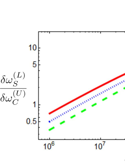
Figure 7: Plot of $\delta\omega_{S}^{(L)}/\delta\omega_{C}^{(U)}$ against the number $N=8k$ of qubits required to extract a single two-qubit state that is close to the Bell pair by the random-sampling test where we set $\delta=10^{-6}$ and $\Delta=0$. Although the horizontal axis represents discrete values, we use continuous lines for plots as guides for the eyes.

V Possible experimental realization

We discuss possible experimental realizations of our protocol. To implement our protocol, we need a solid state system that has a strong coupling with the target fields. Also, a quantum transducer from the solid state system to photons is required to generate a Bell pair between the client and the server. There are several systems that satisfy these requirements.

Nitrogen vacancy (NV) center in diamond is one of the candidates to realize our protocol Maze et al. (2008); Taylor et al. (2008); Balasubramanian et al. (2008); Collins (1994); Gruber et al. (1997); Jelezko et al. (2002). NV centers provide us with a spin triplet, and we can use this system as an effective two level system by using frequency selectivity. Microwave pulses allow us to implement single-qubit gate operations of the NV centers Jelezko et al. (2004). We can readout the state of the NV centers through photoluminescence detection Jiang et al. (2009). On top of these properties, the NV centers have a coupling with magnetic fields, and so the NV centers can be used to measure magnetic fields with a high sensitivity Maze et al. (2008); Taylor et al. (2008); Balasubramanian et al. (2008). Moreover, the NV centers are considered as a candidate to realize a distributed quantum computer and a quantum repeater Barrett and Kok (2005); Childress et al. (2006); Nemoto et al. (2014, 2016). Actually, an entanglement between the NV center and a flying photon can be generated with the current technology Togan et al. (2010). These properties are prerequisite for the possible realization of our protocol.

Moreover, there is a practical motivation to use our scheme of a delegated quantum sensor with the NV center. It is preferable to fabricate a smaller sensor to improve the spatial resolution. Although many efforts have been made to create the NV center in a small nanodiamond Rondin et al. (2012); Cuche et al. (2009); Balasubramanian et al. (2008); Maletinsky et al. (2012), the fabrication of the small nanodiamond containing an NV center is not a mature technology yet. So the client who wants to measure the sample with a high spatial resolution can delegate the sensing to the server who is capable of fabricating such a nanodimaond with a NV center.

A superconducting flux qubit (FQ) coupled with electron spins would be another candidate to realize our protocol Twamley and Barrett (2010); Marcos et al. (2010); Zhu et al. (2011); Zhu et al. (2014); Matsuzaki et al. (2015). High fidelity gate operations of the FQ are available with the current technology Bylander et al. (2011), and it is possible to implement quantum non-demolition measurements on the FQ Clarke and Wilhelm (2007). Moreover, the FQ can be a sensitive magnetic-field sensor due to the large persistent current of the FQ Bal et al. (2012). It is worth mentioning that the FQ itself does not have a direct coupling with the optical photons. However, the quantum state of the FQ can be transferred to the electron spins Saito et al. (2013), and some of the electron spins such as NV centers or rare-earth doped crystals have a coupling with the photons. By using these properties, it is in principle possible to convert the quantum information encoded in the FQ into the form of the photons Blum et al. (2015); Lai et al. (2018); O’Brien et al. (2014). Although such a quantum transducer from the superconducting qubits to the photons is not experimentally demonstrated yet, such a hybrid approach can also be a candidate to realize our remote sensing protocol in the future.

Also, there would be practical advantage for the client to use our delegation scheme with the FQ. The resonant frequency $\omega_{\rm{FQ}}$ of the FQ can be shifted by the applied magnetic field $B$, and the derivative has a linear relationship with the persistent current $I_{\rm{P}}$ of the FQ such as $d\omega_{\rm{FQ}}/dB\propto I_{\rm{P}}$. So the FQ with a higher persistent current has a better sensitivity as a magnetic field sensor. However, such a realization of the high persistent current requires a special design of the superconducting circuit Paauw et al. (2009); Twamley and Barrett (2010), and not every researcher could fabricate such a sample. In our delegation scheme, if the server has an ability to fabricate such a high persistent current FQ, the client can use the server’s FQ to improve the sensitivity to measure the sample that the client has.

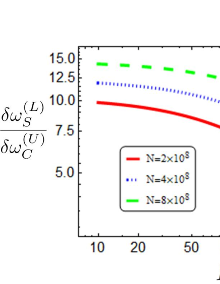
Figure 8: Plot of $\delta\omega_{S}^{(L)}/\delta\omega_{C}^{(U)}$ against the number $M$ of repetitions where we set $\delta=10^{-6}$ and $\Delta=0$. Although the horizontal axis represents discrete values, we use continuous lines for plots as guides for the eyes.

VI Conclusion

We have proposed a delegated quantum sensing protocol. We have considered a situation where the client asks the server to measure the target sample when the client does not have a quantum sensor but the server does. The client provides a sample to be measured with the server, and sends the server the instructions about how to use the quantum sensor to measure the sample. The server obeys the client’s instructions during the measurement of the sample, and will return the sample to the client after the measurement. Importantly, if the standard quantum sensing scheme is naively implemented, not only the client but also the server can obtain the information of the client’s sample even after returning the sample, because of the server’s knowledge of the measurement results. We show that, by using an entanglement between the client and the server, it is possible to realize an asymmetric information gain where only the client can obtain the sufficient information of the sample while the server cannot do it. Our protocol does not require any quantum memory for the client, and so our protocol would be feasible even in the current technology.

However, the resource cost of our protocol is higher than that of the standard quantum sensing protocol, because we need approximately $10^{9}$ qubits in our parameter regime as shown in Fig. 8. As a future work, it is interesting to propose a more resource-efficient quantum remote sensing protocol.

APPENDIX A: PROOF OF THEOREM 2

In this Appendix, we give a proof of Theorem 2.
Proof. The proof is similar to that of Ref. Takeuchi et al. (2018). In order to show this theorem, we use the following inequality:

Lemma 1 (Serfling’s bound Serfling (1974); Tomamichel and Leverrier (2017))

Consider a set of binary random variables $Y=(Y_{1},Y_{2},\ldots,Y_{T})$ with $Y_{j}$ $(1\leq j\leq T)$ taking values in $\{0,1\}$ and $T=N+K$. Then, for any $0<\nu<1$,

$${\rm Pr}\left[\sum_{j\in\bar{\Pi}}Y_{j}\geq\cfrac{N}{K}\sum_{j\in\Pi}Y_{j}+N\nu\right]\leq{\rm exp}\left[-\cfrac{2\nu^{2}NK^{2}}{(N+K)(K+1)}\right],$$

where $\Pi$ is a set of $K$ samples chosen independently and uniformly at random from $Y$ without replacement. $\bar{\Pi}$ is the complementary set of $\Pi$.

Note that the sampling without replacement means that once a sample is selected, it is removed from the population in all subsequent selections.

Let $\Pi^{X}$ and $\Pi^{Z}$ be the sets of $k$ registers used for the $X$ test and the $Z$ test, respectively. In step 3 of the random-sampling test, the client measures $k$ registers of the set $\Pi^{X}$ in the $\hat{\sigma}_{x}\otimes\hat{\sigma}_{x}$ basis. If the $j$th $(1\leq j\leq k)$ register passes the $X$ test, we set $Y_{j}=0$. Otherwise, $Y_{j}=1$. Therefore, by setting $K=k$ and $T=4k$ in Lemma 1, the number $\sum_{j\in\bar{\Pi}^{X}}Y_{j}$ of registers that are not stabilized by $\hat{\sigma}_{x}\otimes\hat{\sigma}_{x}$, where $\bar{\Pi}^{X}$ is the complementary set of $\Pi^{X}$, is upper bounded by

$$3k\nu+3\sum_{j\in\Pi^{X}}Y_{j}$$ (6)

with probability at least

$$1-{\rm exp}\left[-\cfrac{6\nu^{2}k^{3}}{4k(k+1)}\right]\equiv q_{X}.$$ (7)

Next, in step 4 of the random-sampling test, the client measures $k$ registers of the set $\Pi^{Z}$ in the $\hat{\sigma}_{z}\otimes\hat{\sigma}_{z}$ basis. Note that since the registers used for the $Z$ test are selected from registers that are not used for the $X$ test, $\bar{\Pi}^{X}\supset\Pi^{Z}$. By setting $Y_{j}$ in the similar manner to the case of the $X$ test, and setting $K=k$ and $T=3k$ in Lemma 1, the number $\sum_{j\in\bar{\Pi}^{Z}}Y_{j}$ of registers that are not stabilized by $\hat{\sigma}_{z}\otimes\hat{\sigma}_{z}$, where $\bar{\Pi}^{Z}$ is the set of remaining $2k$ registers, is upper bounded by

$$2k\nu+2\sum_{j\in\Pi^{Z}}Y_{j}$$ (8)

with probability at least

$$1-{\rm exp}\left[-\cfrac{4\nu^{2}k^{3}}{3k(k+1)}\right]\equiv q_{Z}.$$ (9)

We set $\nu=2(\epsilon-3\Delta)/5$. From Eqs. (6), (7), (8), and (9), we can guarantee that among the remaining $2k$ registers, at least

$$(4k-2k)-\left(3k\nu+3\sum_{j\in\Pi^{X}}Y_{j}\right)-\left(2k\nu+2\sum_{j\in\Pi^{Z}}Y_{j}\right)$$ (10)

$$= 2k-5k\nu-3\sum_{j\in\Pi^{X}}Y_{j}-2\sum_{j\in\Pi^{Z}}Y_{j}$$

$$\geq 2k-5k\nu-{\color[rgb]{0,0,0}3N_{\rm fail}}$$

$$= 2k-2k(\epsilon-3\Delta)-{\color[rgb]{0,0,0}3N_{\rm fail}}$$

$$= 2k{\color[rgb]{0,0,0}\left(1-\epsilon+3\Delta-\cfrac{3N_{\rm fail}}{2k}\right)}$$

registers always pass the $X$ test and the $Z$ test simultaneously with probability at least

$$q_{X}q_{Z}$$

$$= \left[1-{\rm exp}\left(-\cfrac{3}{2}\nu^{2}k\cfrac{1}{1+1/k}\right)\right]$$

$$\times\left[1-{\rm exp}\left(-\cfrac{4}{3}\nu^{2}k\cfrac{1}{1+1/k}\right)\right]$$

$$\geq \left[1-{\rm exp}\left(-\cfrac{3}{4}\nu^{2}k\right)\right]\left[1-{\rm exp}\left(-\cfrac{2}{3}\nu^{2}k\right)\right]$$

$$\geq 1-2{\rm exp}\left(-\cfrac{2}{3}\nu^{2}k\right)$$

$$\geq 1-2{\rm exp}\left(-\log{\cfrac{2}{\delta}}\right)$$ (12)

$$= 1-\delta,$$ (13)

where we have used $k>1$ and Eq. (2) to derive Eqs. (APPENDIX A: PROOF OF THEOREM 2) and (12), respectively. Only the ideal Bell pair $|\Phi^{+}\rangle$ can always passes both of the $X$ test and the $Z$ test. Therefore, from Eq. (10), the ratio of the number of the ideal Bell pairs to that of non-ideal two-qubit quantum states in the remaining $2k$ registers is at least

$${\color[rgb]{0,0,0}\cfrac{2k\left[1-\epsilon+3\Delta-3N_{\rm fail}/(2k)\right]}{2k}=1-\epsilon+3\Delta-\cfrac{3N_{\rm fail}}{2k}}.$$ (14)

Let

$$\Bigg{\{}|\beta_{ij}\rangle\equiv(\hat{\sigma}_{z}^{i}\otimes\openone)(\hat{\sigma}_{x}^{j}\otimes\openone)\cfrac{|00\rangle+|11\rangle}{\sqrt{2}}\Bigg{|}i,j\in\{0,1\}\Bigg{\}}$$

be the Bell basis. The uniform random selection in step 5 is equivalent to selecting the first register of the remaining $2k$ registers after the random permutation. Therefore, Eqs. (13) and (14) mean that when the state $\rho_{\rm tgt}$ is expanded by the Bell basis:

$$\rho_{\rm tgt}=\sum_{i,j}\sum_{i^{\prime},j^{\prime}}q_{iji^{\prime}j^{\prime}}|\beta_{ij}\rangle\langle\beta_{i^{\prime}j^{\prime}}|,$$

where $\sum_{i,j}q_{ijij}=1$, the coefficient $q_{0000}$ is at least $1-\epsilon+3\Delta-3N_{\rm fail}/(2k)$ with probability at least $1-\delta$. Accordingly, from $|\beta_{00}\rangle=|\Phi^{+}\rangle$ and $\langle\beta_{ij}|\Phi^{+}\rangle=0$ for any $(i,j)\neq(0,0)$,

$$\langle\Phi^{+}|\rho_{\rm tgt}|\Phi^{+}\rangle\geq 1-\epsilon{\color[rgb]{0,0,0}+3\Delta-\cfrac{3N_{\rm fail}}{2k}}$$

with probability at least $1-\delta$. $\blacksquare$

APPENDIX B: PROOF OF THEOREM 3

In this Appendix, we give a proof of Theorem 3.
Proof. First, let us describe a general theory about how to derive the uncertainty of the estimation. Suppose that a state $\rho_{\omega}$, which is the $|+\rangle$ state in the standard quantum metrology, is given, and this state is measured by a projective measurement. We here assume that the probability has a linear dependence on $\omega$. Therefore, we have

$$P={\rm{Tr}}[\hat{\mathcal{P}}\rho_{\omega}]=x+y\omega.$$

If $M$ copies of the state $\rho_{\omega}$ are given, one can measure the state $M$ times and obtain $M$ measurement results $\{m_{j}\}_{j=1}^{M}$, where $m_{j}\in\{0,1\}$. From the average value $S_{M}=(\sum_{j=1}^{M}m_{j})/M$, one can estimate the value of $\omega$ such as $\omega^{(\rm{est})}_{M}=(S_{M}-x)/y$. However, if an unknown error occurs, the actual given state might be $\rho^{\prime}_{\omega}$ that is different from $\rho_{\omega}$, and we consider this case. Suppose that the probability for this state is described as

$$P^{\prime}={\rm{Tr}}[\hat{\mathcal{P}}\rho^{\prime}_{\omega}]=x^{\prime}+y^{\prime}\omega,$$

and this is the actual probability in this case. Furthermore, the average value becomes $S^{\prime}_{M}=(\sum_{j=1}^{M}m^{\prime}_{j})/M$, where $m^{\prime}_{j}(\in\{0,1\})$ is the measurement result obtained from the $j$th copy of $\rho^{\prime}_{\omega}$. Let ${\omega^{\prime}}_{M}^{({\rm est})}\equiv(S^{\prime}_{M}-x)/y$. From the difference between $P$ and $P^{\prime}$, we have

$$\delta^{2}P^{\prime} \equiv M\langle(S^{\prime}_{M}-P^{\prime})^{2}\rangle$$

$$= M\langle(x+y{\omega^{\prime}}_{M}^{(\rm{est})}-x^{\prime}-y^{\prime}\omega)^{2}\rangle$$

$$= M\left\langle\left[\left(x-x^{\prime}\right)+y({\omega^{\prime}}_{M}^{(\rm{est})}-\omega)+(y-y^{\prime})\omega\right]^{2}\right\rangle.$$

So we obtain

$$\delta\omega_{C}$$

$$= \sqrt{\langle({\color[rgb]{0,0,0}{\omega^{\prime}}_{M}^{(\rm{est})}}-\omega)^{2}\rangle}$$

$$= \sqrt{\frac{\frac{\delta^{2}P^{\prime}}{M}+(x-x^{\prime})^{2}+(y-y^{\prime})^{2}\omega^{2}+2(x-x^{\prime})(y-y^{\prime})\omega}{y^{2}}}$$

where we have used $\langle{\omega^{\prime}}^{(\rm{est})}\rangle=(\langle S^{\prime}_{M}\rangle-x)/y=(x^{\prime}+y^{\prime}\omega-x)/y$. By considering small $\omega$, we obtain

$$\delta\omega_{\rm{C}}\simeq\frac{1}{y}\sqrt{\frac{\delta^{2}P^{\prime}}{M}+(x-x^{\prime})^{2}}.$$ (15)

Next, we adopt the above general theory to calculate the uncertainty of the client in our protocol. We define $\rho_{0}\equiv\sum_{s=0,1}p_{s}\hat{\sigma}_{z}^{s}\rho^{(s)}\hat{\sigma}_{z}^{s}$, and we obtain $F\equiv\langle+|\rho_{0}|+\rangle\geq 1-\epsilon$ with probability at least $1-\delta$ from Corollary 1. Since any single-qubit state can be written by a sum of Pauli matrices, we obtain

$$\rho_{0}=\cfrac{\openone+r_{x}\hat{\sigma}_{x}+r_{y}\hat{\sigma}_{y}+r_{z}\hat{\sigma}_{z}}{2},$$

where $r_{x}$, $r_{y}$, and $r_{z}$ are real values such that $r_{x}^{2}+r_{y}^{2}+r_{z}^{2}\leq 1$. We can derive the upper bound $\delta\omega_{C}^{(U)}$ of the client’s uncertainty by optimizing the values of $r_{x}$, $r_{y}$, and $r_{z}$ under the condition that $F\geq 1-\epsilon$. From

$$F=\langle+|\rho_{0}|+\rangle=\frac{1}{2}+\frac{r_{x}}{2}\geq 1-\epsilon,$$

we obtain $r_{x}\geq 1-2\epsilon$ and $r_{y}^{2}\leq 1-r_{x}^{2}-r_{z}^{2}\leq 1-r_{x}^{2}\leq 1-(1-2\epsilon)^{2}=4\epsilon-4\epsilon^{2}$. We here assume that $\epsilon<1/2$. On the other hand, from Eq. (1), the time evolution is described by

$$\rho(t)\simeq\rho_{0}-i\frac{\omega t}{2}[\hat{\sigma}_{z},\rho_{0}]$$

where we consider a small $\omega$. Therefore, we have

$${\rm{Tr}}[\rho(t)\hat{\sigma}_{y}]\simeq r_{y}+\omega tr_{x}.$$

So we obtain

$$P^{\prime}={\rm{Tr}}\left[\frac{\openone+\hat{\sigma}_{y}}{2}\rho(t)\right]\simeq\frac{1+r_{y}+\omega tr_{x}}{2}.$$ (16)

Since $\delta^{2}P^{\prime}=P^{\prime}(1-P^{\prime})$, from Eqs. (15) and (16),

$$\delta^{2}\omega_{C}=\frac{1}{y^{2}}\left[\frac{\delta^{2}P^{\prime}}{M}+(x-x^{\prime})^{2}\right]\leq\frac{1}{t^{2}}\left[\frac{1}{M}+4(\epsilon-\epsilon^{2})\right],$$

where we have used $x=1/2$, $y=t/2$, $x^{\prime}=(1+r_{y})/2$, and $|r_{y}|\leq 2\sqrt{\epsilon-\epsilon^{2}}$. So we obtain

$$\delta\omega^{(U)}_{C}=\frac{1}{t}\sqrt{\frac{1}{M}+4\left(\epsilon-\epsilon^{2}\right)}$$

as the upper bound on the estimation error for the client. The above argument is true if $\langle+|\rho_{0}|+\rangle\geq 1-\epsilon$ holds for all $M$ repetitions. Since this holds with probability at least $1-\delta$ for each repetition, and each repetition is assumed to be independent from the other repetiions, the above argument is true with probability at least $(1-\delta)^{M}$. $\blacksquare$

APPENDIX C: PROOF OF THEOREM 4

In this Appendix, we give a proof of Theorem 4.
Proof. We can describe the single-qubit state $\rho_{\rm\color[rgb]{0,0,0}QRS}$ of the server as follows:

$$\rho_{\rm\color[rgb]{0,0,0}QRS}=\cfrac{\openone+R_{x}\hat{\sigma}_{x}+R_{y}\hat{\sigma}_{y}+R_{z}\hat{\sigma}_{z}}{2}.$$

Let $F(\openone/2,\rho_{\rm QRS})$ be the fidelity between $\openone/2$ and $\rho_{\rm QRS}$. We derive the lower bound $\delta\omega_{S}^{(L)}$ of the server’s uncertainty by optimizing the values of $R_{x}$, $R_{y}$, and $R_{z}$ under the condition that $F(\openone/2,\rho_{\rm\color[rgb]{0,0,0}QRS})\geq 1-\epsilon$. From Eq. (1), we have

$$P = {\rm{Tr}}\left[e^{-i\hat{\mathcal{H}}t{\color[rgb]{0,0,0}/\hbar}}\rho_{\rm\color[rgb]{0,0,0}QRS}e^{i\hat{\mathcal{H}}t{\color[rgb]{0,0,0}/\hbar}}\frac{\openone+\hat{\sigma}_{y}}{2}\right]$$ (17)

$$= \frac{1+R_{y}\cos\omega t+R_{x}\sin\omega t}{2}$$

$$\simeq \frac{1+R_{y}+R_{x}\omega t}{2}$$

for a small $\omega$. In the polar coordinate, we consider $R_{x}=R\sin\theta\cos\phi$, $R_{y}=R\sin\theta\sin\phi$, and $R_{z}=R\cos\theta$, where $R\equiv\sqrt{R_{x}^{2}+R_{y}^{2}+R_{z}^{2}}$, $0\leq\theta\leq\pi$, and $0\leq\phi<2\pi$, On the other hand, we obtain

$$F(\openone/2,\rho_{\rm QRS})=\frac{1}{2}+\frac{1}{2}\sqrt{1-R^{2}}\geq 1-\epsilon$$

and so we have $2\sqrt{\epsilon-\epsilon^{2}}\geq R\geq R_{x}$ and $2\sqrt{\epsilon-\epsilon^{2}}\geq R_{y}$. We assume that the server knows the form of the density matrix $\rho_{\rm QRS}$, and so the server can estimate the value of $\omega$ from the actual form of the probability $P$ unlike the client. From Eqs. (15) and (17),

$$\delta^{2}\omega_{S}\simeq\frac{1}{y^{2}}\frac{\delta^{2}P^{\prime}}{M}\simeq\frac{1-R_{y}^{2}}{t^{2}R_{x}^{2}M}\geq\frac{1-4(\epsilon-\epsilon^{2})}{4t^{2}M(\epsilon-\epsilon^{2})},$$

where we have used $y=tR_{x}/2$, $R_{x}\leq 2\sqrt{\epsilon-\epsilon^{2}}$, and $R_{y}\leq 2\sqrt{\epsilon-\epsilon^{2}}$. So we obtain

$$\delta\omega_{S}^{(L)}=\frac{1}{2t}\sqrt{\frac{1-4(\epsilon-\epsilon^{2})}{M(\epsilon-\epsilon^{2})}}$$

as the lower bound on the uncertainty for the server. The above argument is true if $F(\openone/2,\rho_{\rm QRS})\geq 1-\epsilon$ holds for all $M$ repetitions. Since this holds with probability at least $1-\delta$ for each repetition, and each repetition is assumed to be indepedent from the other repetitions, the above argument is true with probability at least $(1-\delta)^{M}$. $\blacksquare$

APPENDIX D: ANOTHER WAY TO EVALUATE THE UNCERTAINTY OF THE ESTIMATION

In the quantum metrology, it is common to use the variance (or the standard deviation) for the estimation of the accuracy of the sensing protocol. This is the reason why we have adopted this measure to evaluate the asymmetric information gain between the client and server about the sensing results in the main text. However, in some other communities, the variance is not the standard measure but people typically use a statistical inequality.

In this Appendix, we evaluate the uncertainty of the estimation using Hoeffding’s inequality (for details, see Lemma 2). Although such the estimation is not common in the field of the quantum metrology, we include these results especially for the readers who are familiar with statistics.

VI.1 The standard quantum metrology

First, let us consider the simple protocol to measure the target field using a single qubit. The setup is the same as that described in Sec. II. We evaluate a confidence interval for estimaion results of quantum metrology as analyzed in Ref. Sugiyama (2015). We use Hoeffding’s inequality for simplicity, although an empirical Hoeffding inequality was used in Ref. Sugiyama (2015). We also limit the parameter region into a range that the linearization explained in Appendix B is valid. The uncertainty in the approach is defined as

$${\color[rgb]{0,0,0}\Delta}\omega\equiv|\omega^{(\rm{est})}_{M}-\omega|=\frac{2}{t}|S_{M}-P|.$$

To evaluate this uncertainty, we will use the following inequality:

Lemma 2 (Hoeffding’s inequality Hoeffding (1963))

Consider a set of independent random variables $X=(X_{1},X_{2},\ldots,X_{M})$ with $X_{j}$ $(1\leq j\leq M)$ taking values in the interval $[0,1]$. Then, for any $\mu\geq 0$,

$${\rm Pr}\left[\left|\cfrac{1}{M}\sum_{j=1}^{M}X_{j}-\left\langle\cfrac{1}{M}\sum_{j=1}^{M}X_{j}\right\rangle\right|\geq\mu\right]\leq 2e^{-2\mu^{2}M}$$

where $\langle\cdot\rangle$ denotes the expectation value.

From Lemma 2 with $\mu=\tilde{s}/\sqrt{M}$, for any positive $\tilde{s}$ satisfying $e^{-2{\tilde{s}}^{2}}\leq 1/2$,

$${\color[rgb]{0,0,0}\Delta}\omega\leq\frac{2\tilde{s}}{t\sqrt{M}}$$

holds with a probability at least $1-2e^{-2\tilde{s}^{2}}$.

VI.2 Uncertainty of the client

We will explain how to derive the uncertainty of the client using Hoeffding’s inequality. The setup is the same as that described in Sec. IV.2. First, let us consider a general case. While one estimates the value of $\omega$ based on the ideal probability

$$P={\rm{Tr}}[\hat{\mathcal{P}}\rho_{\omega}]=x+y\omega,$$

the actual probability (that may be deviated from the ideal one due to unknown errors) is described as

$$P^{\prime}={\rm{Tr}}[\hat{\mathcal{P}}\rho^{\prime}_{\omega}]=x^{\prime}+y^{\prime}\omega.$$

We can calculate the uncertainty as follows:

$${\color[rgb]{0,0,0}\Delta}\omega$$

$$\equiv |{\omega^{\prime}}^{(\rm{est})}_{M}-\omega|$$

$$= \left|\frac{S^{\prime}_{M}-x}{y}-\frac{P^{\prime}-x^{\prime}}{y^{\prime}}\right|$$

$$= \left|\frac{y^{\prime}S^{\prime}_{M}-yP^{\prime}-xy^{\prime}+x^{\prime}y}{yy^{\prime}}\right|$$

$$= \left|\frac{y^{\prime}S^{\prime}_{M}-yS^{\prime}_{M}+yS^{\prime}_{M}-yP^{\prime}+x^{\prime}y-xy+xy-xy^{\prime}}{yy^{\prime}}\right|$$

$$\leq \frac{|y^{\prime}-y||S^{\prime}_{M}|+|y||S^{\prime}_{M}-P^{\prime}|+|y||x^{\prime}-x|+|x||y-y^{\prime}|}{|yy^{\prime}|}$$

Next, we adopt the above general theory to calculate the uncertainty $\Delta\omega_{C}$ of the client. We have $x=1/2$, $y=t/2$, $x^{\prime}=(1+r_{y})/2$, $y^{\prime}=tr_{x}/2$, $r_{x}\geq 1-2\epsilon$, $|r_{y}|\leq 2\sqrt{\epsilon-\epsilon^{2}}$, $|y-y^{\prime}|\leq|t\epsilon|$, and $|x-x^{\prime}|\leq\sqrt{\epsilon-\epsilon^{2}}$. By substituting these into Eq. (LABEL:newformula), we obtain

$${\color[rgb]{0,0,0}\Delta}\omega_{C}$$ (19)

$$= |{\omega^{\prime}}_{M}^{\rm{(est)}}-\omega|$$

$$\leq \frac{|y^{\prime}-y||S^{\prime}_{M}|+|y||S^{\prime}_{M}-P^{\prime}|+|y||x^{\prime}-x|+|x||y-y^{\prime}|}{|yy^{\prime}|}$$

$$\leq \frac{2}{t(1-2\epsilon)}(2\epsilon|S^{\prime}_{M}|+|S^{\prime}_{M}-P^{\prime}|+\sqrt{\epsilon-\epsilon^{2}}+\epsilon)$$

$$\leq \frac{2}{t(1-2\epsilon)}(3\epsilon+|S^{\prime}_{M}-P^{\prime}|+\sqrt{\epsilon-\epsilon^{2}}).$$

The above argument is true with probability at least $(1-\delta)^{M}$ from the same reason as Appendix B.

We will use the inequality described in Lemma 2 with Eq. (19), and we obtain, for any positive $\tilde{s}$ satisfying $e^{-2{\tilde{s}}^{2}}\leq 1/2$,

$${\color[rgb]{0,0,0}\Delta}\omega_{\color[rgb]{0,0,0}C}\leq\frac{2}{t(1-2\epsilon)}\left(3\epsilon+\frac{\tilde{s}}{\sqrt{M}}+\sqrt{\epsilon-\epsilon^{2}}\right){\color[rgb]{0,0,0}\equiv{\color[rgb]{0,0,0}\Delta}\omega_{C}^{(U)}}$$

with a probability at least $(1-2e^{-2\tilde{s}^{2}})(1-\delta)^{M}$, where we choose $\mu=\tilde{s}/\sqrt{M}$.

As we explained above, the actual probability $P^{\prime}$ is not known for the client, and this lack of the knowledge induces a residual error that is not reduced by increasing the number $M$ of the repetitions.

VI.3 Uncertainty of the server

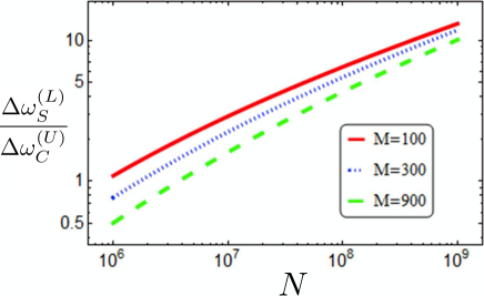
Figure 9: Plot of ${\color[rgb]{0,0,0}\Delta}\omega_{S}^{(L)}/{\color[rgb]{0,0,0}\Delta}\omega_{C}^{(U)}$ against the number $N=8k$ of qubits required to extract a single two-qubit state that is close to the Bell pair by the random-sampling test where we set $\delta=10^{-6}$, $\Delta=0$, and $\tilde{s}=2$ Although the horizontal axis represents discrete values, we use continuous lines for plots as guides for the eyes.

From Eqs. (17) and (LABEL:newformula), we obtain ${\color[rgb]{0,0,0}\Delta}\omega_{S}\equiv|\omega^{\rm{(est)}}_{M}-\omega|=2|S_{M}-P|/(R_{x}t)$. Since we consider the worst case where the server obtains the largest amount of the information, it is natural to choose the parameter $R_{x}$ that minimizes the uncertainty $\Delta\omega_{S}$ of the server. As a result, we have

$$\min{\color[rgb]{0,0,0}\Delta}\omega_{S}=\frac{|S_{M}-P|}{t\sqrt{\epsilon-\epsilon^{2}}}$$ (20)

where we have used $R_{x}\leq 2\sqrt{\epsilon-\epsilon^{2}}$. This argument is tru with probability at least $(1-\delta)^{M}$ from the same reason as Appendix C.

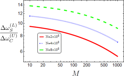
Figure 10: Plot of ${\color[rgb]{0,0,0}\Delta}\omega_{S}^{(L)}/{\color[rgb]{0,0,0}\Delta}\omega_{C}^{(U)}$ against the number $M$ of repetitions where we set $\delta=10^{-6}$, $\Delta=0$, and $\tilde{s}=2$. Although the horizontal axis represents discrete values, we use continuous lines for plots as guides for the eyes.

When the server tries to estimate the value of $\omega$ with the optimal state, the server obtains the uncertainty described in Eq. (20). Then, the server needs to choose a statistical inequality to evaluate $|S_{M}-P|$. Although there are many choices, we consider a case of Hoeffing’s inequality. By using Lemma 2, we obtain, for any positive $\tilde{s}$ satisfying $e^{-2\tilde{s}^{2}}\leq 1/2$,

$$\min{\color[rgb]{0,0,0}\Delta}\omega_{S}\leq\frac{\tilde{s}}{t\sqrt{M}\sqrt{\epsilon-\epsilon^{2}}}{\color[rgb]{0,0,0}\equiv{\color[rgb]{0,0,0}\Delta}\omega_{S}^{(L)}}$$ (21)

with a probability $(1-2e^{-2\tilde{s}^{2}})(1-\delta)^{M}$. It is worth mentioning that, if the server could use another inequality, the server might achieve a better value than that described in Eq. (21). However, finding the best inequality for the server is beyond the scope of this paper, and so we leave this point as a future work.

VI.4 Comparison between the client and server

We compare the uncertainty of the client and that of the server. We plot the ratio ${\color[rgb]{0,0,0}\Delta}\omega_{S}^{(L)}/{\color[rgb]{0,0,0}\Delta}\omega_{C}^{(U)}$ against $N=8k$ in Fig. 9. As we increase $N$, we can increase the ratio ${\color[rgb]{0,0,0}\Delta}\omega_{S}^{(L)}/{\color[rgb]{0,0,0}\Delta}\omega_{C}^{(U)}$, and so the information gain becomes more asymmetric. Also, we plot the ratio ${\color[rgb]{0,0,0}\Delta}\omega_{S}^{(L)}/{\color[rgb]{0,0,0}\Delta}\omega_{C}^{(U)}$ against $M$ in Fig. 10. As we increase the number $M$ of repetitions, the uncertainty of the client becomes closer to that of the server, because the client does not know the precise form of the probability $P^{\prime}$. These results qualitatively agree with the results shown in Figs. 7 and 8 where we use the standard deviation for the evaluation.

References

- Shor (1997) P. W. Shor, SIAM J. Comput. 26, 1484 (1997).
- Grover (1997) L. K. Grover, Phys. Rev. Lett. 79, 325 (1997).
- Harrow et al. (2009) A. W. Harrow, A. Hassidim, and S. Lloyd, Phys. Rev. Lett. 103, 150502 (2009).
- Vandersypen et al. (2001) L. M. Vandersypen, M. Steffen, G. Breyta, C. S. Yannoni, M. H. Sherwood, and I. L. Chuang, Nature (London) 414, 883 (2001).
- Bennett and Brassard (1984) C. H. Bennett and G. Brassard, in Proceedings of IEEE International Conference on Computers, Systems, and Signal Processing (IEEE, New York, 1984), p. 175.
- Bennett et al. (1992) C. H. Bennett, F. Bessette, G. Brassard, L. Salvail, and J. Smolin, Journal of cryptology 5, 3 (1992).
- Gisin et al. (2002) N. Gisin, G. Ribordy, W. Tittel, and H. Zbinden, Reviews of modern physics 74, 145 (2002).
- Broadbent et al. (2009) A. Broadbent, J. Fitzsimons, and E. Kashefi, in Proceedings of the 50th Annual Symposium on Foundations of Computer Science (IEEE, Los Alamitos, 2009), p. 517.
- Morimae and Fujii (2013) T. Morimae and K. Fujii, Phys. Rev. A 87, 050301(R) (2013).
- Takeuchi et al. (2016) Y. Takeuchi, K. Fujii, R. Ikuta, T. Yamamoto, and N. Imoto, Phys. Rev. A 93, 052307 (2016).
- Barz et al. (2012) S. Barz, E. Kashefi, A. Broadbent, J. F. Fitzsimons, A. Zeilinger, and P. Walther, Science 335, 303 (2012).
- Greganti et al. (2016) C. Greganti, M.-C. Roehsner, S. Barz, T. Morimae, and P. Walther, New Journal of Physics 18, 013020 (2016).
- Dowling and Milburn (2003) J. P. Dowling and G. J. Milburn, Philos. Trans. R. Soc. London A 361, 1655 (2003).
- Spiller et al. (2005) T. P. Spiller, W. J. Munro, S. D. Barrett, and P. Kok, Contemp. Phys. 46, 407 (2005).
- Degen et al. (2016) C. Degen, F. Reinhard, and P. Cappellaro, arXiv:1611.02427 (2016).
- Budker and Romalis (2007) D. Budker and M. Romalis, Nat. Phys. 3, 227 (2007).
- Balasubramanian et al. (2008) G. Balasubramanian et al., Nature (London) 455, 648 (2008).
- Maze et al. (2008) J. Maze et al., Nature (London) 455, 644 (2008).
- Dolde et al. (2011) F. Dolde et al., Nat. Phys. 7, 459 (2011).
- Neumann et al. (2013) P. Neumann et al., Nano letters 13, 2738 (2013).
- Wineland et al. (1992) D. J. Wineland, J. J. Bollinger, W. M. Itano, F. L. Moore, and D. J. Heinzen, Phys. Rev. A 46, R6797(R) (1992).
- Huelga et al. (1997) S. F. Huelga, C. Macchiavello, T. Pellizzari, A. K. Ekert, M. B. Plenio, and J. I. Cirac, Phys. Rev. Lett. 79, 3865 (1997).
- Matsuzaki et al. (2011) Y. Matsuzaki, S. C. Benjamin, and J. Fitzsimons, Phys. Rev. A 84, 012103 (2011).
- Chin et al. (2012) A. W. Chin, S. F. Huelga, and M. B. Plenio, Phys. Rev. Lett. 109, 233601 (2012).
- Kessler et al. (2014) E. M. Kessler, I. Lovchinsky, A. O. Sushkov, and M. D. Lukin, Phys. Rev. Lett. 112, 150802 (2014).
- Dür et al. (2014) W. Dür, M. Skotiniotis, F. Fröwis, and B. Kraus, Phys. Rev. Lett. 112, 080801 (2014).
- Arrad et al. (2014) G. Arrad, Y. Vinkler, D. Aharonov, and A. Retzker, Phys. Rev. Lett. 112, 150801 (2014).
- Herrera-Martí et al. (2015) D. A. Herrera-Martí, T. Gefen, D. Aharonov, N. Katz, and A. Retzker, Phys. Rev. Lett. 115, 200501 (2015).
- Unden et al. (2016) T. Unden et al., Phys. Rev. Lett. 116, 230502 (2016).
- Matsuzaki and Benjamin (2017) Y. Matsuzaki and S. Benjamin, Phys. Rev. A 95, 032303 (2017).
- Higgins et al. (2007) B. L. Higgins, D. W. Berry, S. D. Bartlett, H. M. Wiseman, and G. J. Pryde, Nature (London) 450, 393 (2007).
- Waldherr et al. (2012) G. Waldherr, J. Beck, P. Neumann, R. Said, M. Nitsche, M. Markham, D. Twitchen, J. Twamley, F. Jelezko, and J. Wrachtrup, Nat. Nanotechnol. 7, 105 (2012).
- Nakayama et al. (2015) S. Nakayama, A. Soeda, and M. Murao, Phys. Rev. Lett. 114, 190501 (2015).
- Matsuzaki et al. (2017) Y. Matsuzaki, S. Nakayama, A. Soeda, S. Saito, and M. Murao, Phys. Rev. A 95, 062106 (2017).
- Komar et al. (2014) P. Komar, E. M. Kessler, M. Bishof, L. Jiang, A. S. Sørensen, J. Ye, and M. D. Lukin, Nat. Phys. 10, 582 (2014).
- Eldredge et al. (2018) Z. Eldredge, M. Foss-Feig, J. A. Gross, S. L. Rolston, and A. V. Gorshkov, Phys. Rev. A 97, 042337 (2018).
- Proctor et al. (2018) T. J. Proctor, P. A. Knott, and J. A. Dunningham, Phys. Rev. Lett. 120, 080501 (2018).
- Lidar and Brun (2013) D. A. Lidar and T. A. Brun, Quantum error correction (Cambridge University Press, Cambridge, 2013).
- Kitaev (1996) A. Y. Kitaev, Electronic Colloquium on Computational Complexity 3, 3 (1996).
- Sasaki et al. (2011) M. Sasaki et al., Optics express 19, 10387 (2011).
- Wang et al. (2013) J.-Y. Wang et al., Nat. Photon. 7, 387 (2013).
- Giovannetti et al. (2001) V. Giovannetti, S. Lloyd, and L. Maccone, Nature (London) 412, 417 (2001).
- Giovannetti et al. (2002a) V. Giovannetti, S. Lloyd, and L. Maccone, J. Opt. B: Quantum Semiclassical Opt. 4, S413 (2002a).
- Giovannetti et al. (2002b) V. Giovannetti, S. Lloyd, and L. Maccone, Phys. Rev. A 65, 022309 (2002b).
- Chiribella et al. (2005) G. Chiribella, G. M. D’Ariano, and M. F. Sacchi, Phys. Rev. A 72, 042338 (2005).
- Chiribella et al. (2007) G. Chiribella, L. Maccone, and P. Perinotti, Phys. Rev. Lett. 98, 120501 (2007).
- Huang et al. (2017) Z. Huang, C. Macchiavello, and L. Maccone, arXiv:1706.03894 (2017).
- Xie et al. (2018) D. Xie, C. Xu, J. Chen, and A. M. Wang, Quant. Info. Proc. 17, 116 (2018).
- Bennett et al. (1993) C. H. Bennett, G. Brassard, C. Crépeau, R. Jozsa, A. Peres, and W. K. Wootters, Phys. Rev. Lett. 70, 1895 (1993).
- Bouwmeester et al. (1997) D. Bouwmeester, J.-W. Pan, K. Mattle, M. Eibl, H. Weinfurter, and A. Zeilinger, Nature (London) 390, 575 (1997).
- Furusawa et al. (1998) A. Furusawa, J. L. Sørensen, S. L. Braunstein, C. A. Fuchs, H. J. Kimble, and E. S. Polzik, Science 282, 706 (1998).
- Julsgaard et al. (2004) B. Julsgaard, J. Sherson, J. I. Cirac, J. Fiurášek, and E. S. Polzik, Nature (London) 432, 482 (2004).
- Hedges et al. (2010) M. P. Hedges, J. J. Longdell, Y. Li, and M. J. Sellars, Nature (London) 465, 1052 (2010).
- Smithey et al. (1993) D. T. Smithey, M. Beck, M. G. Raymer, and A. Faridani, Phys. Rev. Lett. 70, 1244 (1993).
- Hradil (1997) Z. Hradil, Phys. Rev. A 55, R1561 (1997).
- Banaszek et al. (1999) K. Banaszek, G. M. D’Ariano, M. G. A. Paris, and M. F. Sacchi, Phys. Rev. A 61, 010304 (1999).
- Poyatos et al. (1997) J. F. Poyatos, J. I. Cirac, and P. Zoller, Phys. Rev. Lett. 78, 390 (1997).
- Chuang and Nielsen (1997) I. L. Chuang and M. A. Nielsen, J. Mod. Opt. 44, 2455 (1997).
- Nielsen and Chuang (2000) M. A. Nielsen and I. L. Chuang, Quantum Computation and Quantum Information (Cambridge University Press, Cambridge, 2000).
- Takeuchi et al. (2018) Y. Takeuchi, A. Mantri, T. Morimae, A. Mizutani, and J. F. Fitzsimons, arXiv:1806.09138 (2018).
- Hayashi and Morimae (2015) M. Hayashi and T. Morimae, Phys. Rev. Lett. 115, 220502 (2015).
- Markham and Krause (2018) D. Markham and A. Krause, arXiv:1801.05057 (2018).
- Taylor et al. (2008) J. Taylor, P. Cappellaro, L. Childress, L. Jiang, D. Budker, P. Hemmer, A. Yacoby, R. Walsworth, and M. Lukin, Nat. Phys. 4, 810 (2008).
- Collins (1994) A. T. Collins, Properties and Growth of Diamond, edited by G. Davies (INSPEC, London, 1994).
- Gruber et al. (1997) A. Gruber, A. Dräbenstedt, C. Tietz, L. Fleury, J. Wrachtrup, and C. Von Borczyskowski, Science 276, 2012 (1997).
- Jelezko et al. (2002) F. Jelezko, I. Popa, A. Gruber, C. Tietz, J. Wrachtrup, A. Nizovtsev, and S. Kilin, Appl. Phys. Lett. 81, 2160 (2002).
- Jelezko et al. (2004) F. Jelezko, T. Gaebel, I. Popa, A. Gruber, and J. Wrachtrup, Phys. Rev. Lett. 92, 076401 (2004).
- Jiang et al. (2009) L. Jiang et al., Science 326, 267 (2009).
- Barrett and Kok (2005) S. D. Barrett and P. Kok, Phys. Rev. A 71, 060310(R) (2005).
- Childress et al. (2006) L. Childress, J. M. Taylor, A. S. Sørensen, and M. D. Lukin, Phys. Rev. Lett. 96, 070504 (2006).
- Nemoto et al. (2014) K. Nemoto, M. Trupke, S. J. Devitt, A. M. Stephens, B. Scharfenberger, K. Buczak, T. Nöbauer, M. S. Everitt, J. Schmiedmayer, and W. J. Munro, Phys. Rev. X 4, 031022 (2014).
- Nemoto et al. (2016) K. Nemoto, M. Trupke, S. J. Devitt, B. Scharfenberger, K. Buczak, J. Schmiedmayer, and W. J. Munro, Sci. Rep. 6, 26284 (2016).
- Togan et al. (2010) E. Togan et al., Nature (London) 466, 730 (2010).
- Rondin et al. (2012) L. Rondin, J. P. Tetienne, P. Spinicelli, C. Dal Savio, K. Karrai, G. Dantelle, A. Thiaville, S. Rohart, J. F. Roch, and V. Jacques, Appl. Phys. Lett. 100, 153118 (2012).
- Cuche et al. (2009) A. Cuche, A. Drezet, Y. Sonnefraud, O. Faklaris, F. Treussart, J.-F. Roch, and S. Huant, Opt. Express 17, 19969 (2009).
- Maletinsky et al. (2012) P. Maletinsky, S. Hong, M. S. Grinolds, B. Hausmann, M. D. Lukin, R. L. Walsworth, M. Loncar, and A. Yacoby, Nat. Nanotechnol. 7, 320 (2012).
- Twamley and Barrett (2010) J. Twamley and S. D. Barrett, Phys. Rev. B 81, 241202 (2010).
- Marcos et al. (2010) D. Marcos, M. Wubs, J. M. Taylor, R. Aguado, M. D. Lukin, and A. S. Sørensen, Phys. Rev. Lett. 105, 210501 (2010).
- Zhu et al. (2011) X. Zhu et al., Nature (London) 478, 221 (2011).
- Zhu et al. (2014) X. Zhu, Y. Matsuzaki, R. Amsuss, K. Kakuyanagi, T. Shimo-Oka, N. Mizuochi, K. Nemoto, W. J. Munro, K. Semba, and S. Saito, Nat. Commun. 3424, 4524 (2014).
- Matsuzaki et al. (2015) Y. Matsuzaki et al., Phys. Rev. Lett. 114, 120501 (2015).
- Bylander et al. (2011) J. Bylander, S. Gustavsson, F. Yan, F. Yoshihara, K. Harrabi, G. Fitch, D. G. Cory, Y. Nakamura, J. S. Tsai, and W. D. Oliver, Nat. Phys. 7, 565 (2011).
- Clarke and Wilhelm (2007) J. Clarke and F. K. Wilhelm, Nature (London) 453, 1031 (2007).
- Bal et al. (2012) M. Bal, C. Deng, J.-L. Orgiazzi, F. Ong, and A. Lupascu, Nat. Commun. 3, 1324 (2012).
- Saito et al. (2013) S. Saito, X. Zhu, R. Amsüss, Y. Matsuzaki, K. Kakuyanagi, T. Shimo-Oka, N. Mizuochi, K. Nemoto, W. J. Munro, and K. Semba, Phys. Rev. Lett. 111, 107008 (2013).
- Blum et al. (2015) S. Blum, C. O’Brien, N. Lauk, P. Bushev, M. Fleischhauer, and G. Morigi, Phys. Rev. A 91, 033834 (2015).
- Lai et al. (2018) Y.-Y. Lai, G.-D. Lin, J. Twamley, and H.-S. Goan, Phys. Rev. A 97, 052303 (2018).
- O’Brien et al. (2014) C. O’Brien, N. Lauk, S. Blum, G. Morigi, and M. Fleischhauer, Phys. Rev. Lett. 113, 063603 (2014).
- Paauw et al. (2009) F. G. Paauw, A. Fedorov, C. J. P. M. Harmans, and J. E. Mooij, Phys. Rev. Lett. 102, 090501 (2009).
- Serfling (1974) R. J. Serfling, Ann. Stat. 2, 39 (1974).
- Tomamichel and Leverrier (2017) M. Tomamichel and A. Leverrier, Quantum 1, 14 (2017).
- Sugiyama (2015) T. Sugiyama, Phys. Rev. A 91, 042126 (2015).
- Hoeffding (1963) W. Hoeffding, Journal of the American Statistical Association 58, 13 (1963).