Improving constant in end-point Poincaré inequality on Hamming cube

Abstract.

We improve the constant $\frac{\pi}{2}$ in $L^{1}$-Poincaré inequality on Hamming cube. For Gaussian space the sharp constant in $L^{1}$ inequality is known, and it is $\sqrt{\frac{\pi}{2}}$. For Hamming cube the sharp constant is not known, and $\sqrt{\frac{\pi}{2}}$ gives an estimate from below for this sharp constant. On the other hand, L. Ben Efraim and F. Lust-Piquard have shown an estimate from above: $C_{1}\leq\frac{\pi}{2}$. There are at least two other independent proofs of the same estimate from above (we write down them in this note). Since those proofs are very different from the proof of Ben Efraim and Lust-Piquard but gave the same constant, that might have indicated that constant is sharp. But here we give a better estimate from above, showing that $C_{1}$ is strictly smaller than $\frac{\pi}{2}$. It is still not clear whether $C_{1}>\sqrt{\frac{\pi}{2}}$. We discuss this circle of questions.

1. Introduction

In [1] the following inequality is proved

(1.1) $$\|f-\mathbb{E}f\|_{1}\leq\frac{\pi}{2}\|\nabla f\|_{1},$$

where $f$ is a function on Hamming cube $\{-1,1\}^{n}$. Pisier proved that in Gaussian space the following Poincaré inequality holds with the sharp constant $\sqrt{\pi/2}$:

(1.2) $$\|f-\mathbb{E}f\|_{1}\leq\sqrt{\frac{\pi}{2}}\|\nabla f\|_{1},$$

If we denote by $C_{1}$ the best constant in the Poincaré inequality in $L^{1}(\{-1,1\}^{n})$, then we see that

$$\sqrt{\frac{\pi}{2}}\leq C_{1}\leq\frac{\pi}{2}\,.$$

In this note we improve the right estimate. Let $\Delta$ be Laplacian on $\{-1,1\}^{n}$ (negative operator). Let $P_{t}:=e^{t\Delta}$ be a corresponding semi-group.

The proof of (1.1) in [1] is striking. To obtain this estimate the authors adapt Pisier’s proof to the Hamming cube. For this they lift the problem about functions to non-commutative problem about matrices. After that they manage to represent operator $P_{t}$ as a compression of a semi-group acting on a non-commutative space of $2^{n}\times 2^{n}$ matrices, and then the rest of the argument relies on the non-commutative Khinthchin inequality. This lifting of a problem about usual functions to a non-commutative setting is immensely beautiful and enticing, but also a bit mysterious.

There are “commutative” proofs of the estimate from above in $L^{1}(\{-1,1\}^{n})$-Poincaré inequality. We present them in Section 7. They give exactly the same constant $\pi/2$ (or worse) as in [1] but they use a sort of “Bellman function” monotonicity idea. We learnt them from the book of Bakry–Gentil–Ledoux [2], Chapter 8.

This persistence of $\pi/2$ constant in three very different proofs could have been suggestive. But here we prove that sharp constant is smaller than $\pi/2$. What it is remains enigmatic.

2. Dual problem

We write a dual problem as follows. Let $f\in L^{1}(\{-1,1\}^{n})$ and $g\in L^{\infty}(\{-1,1\}^{n})$. Let $\mathbb{E}f=0$. Then

$$f-\mathbb{E}f=-\int_{0}^{\infty}\frac{d}{dt}P_{t}f\,dt\,.$$

and hence

$$(f-\mathbb{E}f,g)=-\int_{0}^{\infty}(\Delta P_{t}f,g)\,dt=-\int_{0}^{\infty}(\Delta f,P_{t}g)\,dt=$$

$$-(\Delta f,\int_{0}^{\infty}P_{t}g\,dt)=-(\nabla f,\int_{0}^{\infty}\nabla P_{t}g\,dt)\,.$$

Therefore,

$$\mathbb{E}|f-\mathbb{E}f|\leq\|\nabla f\|_{1}\cdot\sup_{\|g\|_{\infty}\leq 1}\Big{\|}\int_{0}^{\infty}\nabla P_{t}g\,dt\Big{\|}_{\infty}\leq\|\nabla f\|_{1}\cdot\sup_{\|g\|_{\infty}\leq 1}\int_{0}^{\infty}\|\nabla P_{t}g\|_{\infty}\,dt\,.$$

So we will estimate

$$\sup_{\|g\|_{\infty}\leq 1}\int_{0}^{\infty}\|\nabla P_{t}g\|_{\infty}\,dt$$

by $C_{dual}\|g\|_{\infty}$. We will prove that $C_{dual}<\frac{\pi}{2}$. We just showed that $C_{1}\leq C_{dual}$. There is a very good possibility that $C_{1}<C_{dual}$. We discuss that in this note, where we talk about the $Curl$ space–see below in Section 13.

3. Integral operator

Let us consider $g\mapsto\nabla P_{t}g$ as an integral operator and let us write down its kernel. Consider independent random variables $\{y_{1},\dots,y_{n}\}$, which are $\rho$-correlated with standard Bernoulli independent random variables $\{x_{1},\dots,x_{n}\}$. If $y_{i}=x_{i}$ with probability $\frac{1+\rho}{2}$ and $y_{i}=-x_{i}$ with probability $\frac{1-\rho}{2}$, then we have them exactly $\rho$-correlated $\mathbb{E}y_{i}x_{i}=\rho$. Given a fixed string $x\in\{-1,1\}^{n}$, we can write

$$\mathbb{E}_{{\bf y}\sim N_{\rho}(x)}{\bf y}^{S}=\rho^{|S|}x^{S},$$

where $S$ is a multi-index of $0$ and $1$, $x^{S}$ is a corresponding polynomial, and ${\bf y}\sim N_{\rho}(x)$ means distribution $\rho$-correlated independent random variables.

Putting $\rho=e^{-t}$ we get

$$\mathbb{E}_{{\bf y}\sim N_{\rho}(x)}g({\bf y})=(P_{t}g)(x)\,.$$

Since

$$\nabla P_{t}g=e^{-t}P_{t}\nabla g$$

we can apply this to $\partial_{1}g$.

$$(P_{t}\partial_{1}g)(x)=\mathbb{E}_{{\bf y}\sim N_{\rho}(x)}\partial_{1}g({\bf y})\,.$$

Now we want to find $\varphi_{1}({\bf y})$ such that

$$\mathbb{E}_{{\bf y}\sim N_{\rho}(x)}\partial_{1}g({\bf y})=\mathbb{E}_{{\bf y}\sim N_{\rho}(x)}\varphi_{1}({\bf y})g({\bf y})\,.$$

But $\partial_{1}$ eliminates all polynomials that do not have ${\bf y}_{1}$ and cross off ${\bf y}_{1}$ from other polynomials. So $\varphi_{1}$ such that

$$\mathbb{E}_{{\bf y}\sim N_{\rho}(x)}\varphi_{1}({\bf y}){\bf y}_{k}=\delta_{1k}\,.$$

Clearly the following $\varphi_{1}$ works:

$$\varphi_{1}(y)=\frac{y_{1}-\mathbb{E}_{{\bf y}\sim N_{\rho}(x)}{\bf y}_{1}}{Var[{\bf y_{1}}]}=\frac{y_{1}-\rho x_{1}}{1-\rho^{2}}=\frac{y_{1}-e^{-t}x_{1}}{1-e^{-2t}}\,.$$

Combining all that we get the integral representation of $(P_{t}\nabla g)(x)$:

(3.1) $$(P_{t}\nabla g)(x)=\mathbb{E}_{{\bf y}\sim N_{\rho}(x)}\Big{(}(\frac{{\bf y_{1}}-e^{-t}x_{1}}{1-e^{-2t}},\dots,\frac{{\bf y_{n}}-e^{-t}x_{n}}{1-e^{-2t}})g({\bf y})\Big{)}\,.$$

From (3.1) we get ($\lambda=\lambda_{1},\dots,\lambda_{n})$ (a unit vector in $\mathbb{R}^{n}$)

(3.2) $$\|(P_{t}\nabla g)\|_{\infty}\leq\frac{1}{\sqrt{1-e^{-2t}}}\|g\|_{\infty}\left\|\sup_{\lambda:\|\lambda\|_{2}=1}\mathbb{E}_{{\bf y}\sim N_{\rho}(x)}\Big{|}\sum_{j=1}^{n}\lambda_{j}\frac{{\bf y}_{j}-e^{-t}x_{j}}{\sqrt{1-e^{-2t}}}\Big{|}\right\|_{\infty}$$

To estimate the right hand side without loss of generality we can assume that $x_{j}=1$ for all $j=1,\ldots,n$. Indeed, this follows from the fact that we are taking supremum over all $\lambda\in\mathbb{S}^{n-1}$, and since ${\bf y}-e^{-t}x_{j}$ takes values $x_{j}(1-e^{-t})$ and $-x_{j}(1+e^{-t})$ we can absorb the signs $x_{j}$ into the values of $\lambda_{j}$.

The random variables $\frac{{\bf y}_{j}-e^{-t}}{\sqrt{1-e^{-2t}}}$ are independent, and they have the same distribution as random variables $\xi_{i}^{t}$ that assume value $\sqrt{\frac{1-e^{-t}}{1+e^{-t}}}$ with probability $\frac{1+e^{-t}}{2}$ and $-\sqrt{\frac{1+e^{-t}}{1-e^{-t}}}$ with probability $\frac{1-e^{-t}}{2}$.

Hence, for $\|g\|_{\infty}\leq 1$, we have

(3.3) $$\|\nabla(P_{t}g)\|_{\infty}=\frac{e^{-t}}{\sqrt{1-e^{-2t}}}\sup_{\lambda:\|\lambda\|_{2}=1}\big{\|}\sum\lambda_{j}\xi_{j}^{t}\big{\|}_{L^{1}(\mathbb{P})}\,.$$

Notice that $\int\xi_{j}^{t}\,d\mathbb{P}=0$, $\int(\xi_{j}^{t})^{2}\,d\mathbb{P}=1$. Thus, there is a trivial estimate

(3.4) $$\|\nabla(P_{t}g)\|_{\infty}=\frac{e^{-t}}{\sqrt{1-e^{-2t}}}\sup_{\lambda:\|\lambda\|_{2}=1}\big{\|}\sum\lambda_{j}\xi_{j}^{t}\big{\|}_{L^{2}(\mathbb{P})}\leq\frac{e^{-t}}{\sqrt{1-e^{-2t}}}\,.$$

The first estimate here is just (3.3), the second one is just a trivial fact that $\|\sum\lambda_{j}\xi_{j}^{t}\big{\|}_{L^{2}(\mathbb{P})}^{2}=\lambda_{1}^{2}+\dots+\lambda_{n}^{2}=1$.

Using $\int_{0}^{\infty}\frac{e^{-t}}{\sqrt{1-e^{-2t}}}dt=\int_{0}^{1}\frac{du}{\sqrt{1-u^{2}}}=\frac{\pi}{2}$ we see (1.1) one more time.

To improve this estimate it is sufficient to prove the following theorem.

Theorem 3.1.

Let $p\in[\frac{1}{2},1\big{]}$. Consider independent random variables $\varepsilon_{j}$, $j=1,\dots,n$, having values $\sqrt{\frac{1-p}{p}}$ with probability $p$ and $-\sqrt{\frac{p}{1-p}}$ with probability $1-p$. Then $\sup_{\lambda\in\mathbb{R}^{n}:\|\lambda\|_{2}=1}\|\sum\lambda_{j}\varepsilon_{j}\|_{1}=:q(p)<1$ for $p$ lying in a small interval around $3/4$.

Remark 3.2.

In fact, the proof will show that $q(p)<1$ for all $p\in(\frac{1}{2},1)$.

In the next two section we prove this theorem.

Acknowledgement. We are grateful to Sergei Bobkov who indicated to us the article [3]. The proof there, even though it is different from the proof below, encouraged us.

4. Maximum $\lambda$ is separated from $1$

Everything is real-valued below. We will need the $8$-th moment in the calculation below.

Let $\xi_{i}$, $i=1,\dots,n$ be our random Bernoulli variables with $\mathbb{E}\xi=0,\mathbb{E}\xi^{2}=1$, $1-p,p$ probability of values $\sqrt{\frac{p}{1-p}},-\sqrt{\frac{1-p}{p}}$, and independent. Let $\lambda=(\lambda_{1},\dots,\lambda_{n})$ be a point on the unit sphere. In this section we consider the case

(4.1) $$\max|\lambda_{k}|^{2}\leq 0.99\,.$$

We want to prove that independently of $n$ under this assumption above and with a certain $\varepsilon>0$, which will depend only on a constant $p$ chosen later in (4.7), we will have

(4.2) $$\max|\lambda_{k}|^{2}\leq 0.99\Rightarrow\mathbb{E}|\sum\lambda_{i}\xi_{i}|\leq(1-\varepsilon^{2})\big{(}\mathbb{E}(\sum\lambda_{i}\xi_{i})^{2}\big{)}^{1/2}=1-\varepsilon^{2}\,.$$

Denote $Y:=|\sum\lambda_{i}\xi_{i}|$ and notice that if the opposite happens for some $\lambda$ satisfying (4.1), then

$$\mathbb{E}(Y-\mathbb{E}Y)^{2}=1-\big{(}\mathbb{E}Y\big{)}^{2}<1-(1-\varepsilon^{2})^{2}\leq 2\varepsilon^{2}\,.$$

So if (4.2) does not hold, then on a large probability $Y$ is close to $\mathbb{E}Y$ (and $\mathbb{E}Y$ is close to $1$ of course) for certain $\lambda$ satisfying (4.1). Hence, for this $\lambda$,

$$\text{with probability}\quad 1-2\varepsilon\quad\text{one has}\,\,\big{|}|\sum\lambda_{i}\xi_{i}|-1\big{|}^{2}\leq\varepsilon+2\varepsilon^{2}\,.$$

We took here into account that if the opposite to (4.2) happens, then $0\leq 1-\mathbb{E}Y\leq 1-\sqrt{1-2\varepsilon^{2}}$. In particular, we obtain

(4.3) $$P\left(\left||\sum\lambda_{j}\xi_{j}|^{2}-1\right|\leq\sqrt{\varepsilon+2\varepsilon^{2}}(1+\sqrt{\varepsilon+2\varepsilon^{2}})\right)\geq 1-2\varepsilon$$

Now let us bring (4.3) (with a certain $\varepsilon$ chosen below with the help of constant $B$ from (4.5) below) to a contradiction if (4.1) holds.

Consider $\ell=\sum\lambda_{i}\xi_{i}$, then

$$\ell^{2}=\sum\lambda_{i}^{2}\xi_{i}^{2}+2\sum_{i<j}\lambda_{i}\lambda_{j}\xi_{i}\xi_{j}\,.$$

So

$$\ell^{4}=\sum\lambda_{i}^{4}\xi_{i}^{4}+2\sum_{i<j}\lambda_{i}^{2}\lambda_{j}^{2}\xi_{i}^{2}\xi_{j}^{2}+4\sum_{i<j}\lambda_{i}^{2}\lambda_{j}^{2}\xi_{i}^{2}\xi_{j}^{2}+$$

(4.4) $$4\sum_{i<j,k<m,(i,j)\neq(k,m)}\lambda_{i}\lambda_{j}\xi_{i}\xi_{j}\lambda_{k}\lambda_{m}\xi_{k}\xi_{m}\,+4\sum_{m,\,i<j}\lambda_{m}^{2}\xi_{m}^{2}\lambda_{i}\lambda_{j}\xi_{i}\xi_{j}$$

Of course $\mathbb{E}\ell^{2}=1$. Now calculate $Var[\ell^{2}]$. By (4) we have

$$Var[\ell^{2}]=\mathbb{E}(\ell^{2}-1)^{2}=\mathbb{E}\ell^{4}-2\mathbb{E}\ell^{2}+1=\mathbb{E}\ell^{4}-1=$$

$$\mathbb{E}\xi^{4}\sum\lambda_{i}^{4}+6\sum_{i<j}\lambda_{i}^{2}\lambda_{j}^{2}-1\geq\sum\lambda_{j}^{4}+3(1-\sum\lambda_{j}^{4})-1=$$

$$2(1-\sum\lambda_{j}^{4})\geq 2\cdot 0.01=0.02$$

Here we have used $\mathbb{E}\xi^{4}\geq 1$ and $\lambda_{j}^{4}\leq 0.99\lambda_{j}^{2}$ for all $j=1,\ldots,n$.

Let $X:=|\ell^{2}-1|$. If

(4.5) $$\mathbb{E}X^{4}\leq B(\mathbb{E}X^{2})^{2},$$

then the Paley–Zygmund estimate applied to $X^{2}$ says

$$\mathbb{P}(X\geq t(\mathbb{E}X^{2})^{1/2})\geq(1-t^{2})^{2}\frac{1}{B},\quad t\in(0,1)\,.$$

Let us take (4.5) for granted and let us then see what Paley–Zygmund estimate gives us with $t=1/2$. Since we estimated $\mathbb{E}X^{2}$ from below as follows

$$\mathbb{E}X^{2}\geq 0.02$$

we get

(4.6) $$\mathbb{P}(|\ell^{2}-1|\geq 0.07)\geq\mathbb{P}(X\geq\frac{1}{2}\frac{\sqrt{2}}{10})\geq\frac{9}{16}\frac{1}{B}\,.$$

This contradicts (4.3). Indeed, summing up (4.3) and (4.6) we obtain

(4.7) $$\mathbb{P}(|\ell^{2}-1|\geq 0.07)+\mathbb{P}\big{(}|\ell^{2}-1|\leq\sqrt{\varepsilon+2\varepsilon^{2}}(1+\sqrt{\varepsilon+2\varepsilon^{2}})\big{)}\geq\frac{9}{16B}+1-2\varepsilon\,.$$

Now it remains to take $\varepsilon$ sufficiently small to get a contradiction.

So if we prove (4.5) with $B$ depending on $p$ but independent of $n$, we would prove that we have the drop in norm as in (4.2) with $\varepsilon$ sufficiently small depending only on $p$.

To see (4.5) with $B$ independent of $n$ and independent of $\lambda_{i}$ satisfying (4.1), $\sum\lambda_{i}^{2}=1$, let us recall that $X=|\ell^{2}-1|$ and we already estimated $\mathbb{E}X^{2}=\mathbb{E}(\ell^{2}-1)^{2}\geq 0.02$ from below, and this estimate depends only on assumption (4.1).

To prove (4.5) we now just need to estimate $\mathbb{E}X^{4}=\mathbb{E}(\ell^{2}-1)^{4}$ from above by $C(p)<\infty$. For this we need only to estimate $\mathbb{E}\,\ell^{8}$. Looking at (4), we square it and integrate. It is clear then that only sums involving $\lambda_{k}^{2m}$, $m=1,2,3,4$, will survive. It is now easy to see that $\mathbb{E}\,\ell^{8}\leq C(p)$, where $C(p)$ is bounded if we do not make $p\to 1$. This just because $\sum_{j=1}^{n}\lambda_{j}^{2m}\leq 1,\,m=1,2,\dots$, and because of the obvious estimate $\mathbb{E}\,|\xi_{i}|^{2m}\leq K(p,m,\delta)<\infty$ if $p\in[\frac{1}{2},1-\delta\big{)}$.

Hence, we have

(4.8) $$\mathbb{E}X^{4}\leq B(p)(\mathbb{E}X^{2})^{2},\quad B(p)\leq B_{\delta}<\infty,\,\,p\in[1/2,1-\delta\big{)}\,.$$

So for $p=\frac{3}{4}$ and also for $p$ in a small fixed (independent of $n$) neighborhood of $p=\frac{3}{4}$ we have a definite drop in norm. In other words, we have the Hölder inequality with constant strictly smaller than $1$ independently of $n$ and independent of $\lambda$ satisfying (4.1).

5. Maximum is close to $1$

What if the $\max_{k}|\lambda_{k}|^{2}=:\lambda_{1}^{2}$ is in $[0.99,1]$? Here we should think that $p\in(\frac{1}{2}+\delta,1\big{]}$. For example $p$ is in a small fixed interval around $\frac{3}{4}$.

Then we write for $p=\frac{3}{4}$:

$$\mathbb{E}|\sum\lambda_{i}\xi_{i}|\leq\lambda_{1}\mathbb{E}|\xi_{1}|+\mathbb{E}|\sum_{i=2}^{n}\lambda_{i}\xi_{i}|\leq\lambda_{1}\mathbb{E}|\xi_{1}|+\big{(}\mathbb{E}|\sum_{i=2}^{n}\lambda_{i}\xi_{i}|^{2}\big{)}^{1/2}$$

$$\leq 2\sqrt{(1-p)p}+\sqrt{1-\lambda_{1}^{2}}\leq\frac{\sqrt{3}}{2}+\frac{1}{10}<0.87+0.1=0.97.$$

Again we have a fixed drop in Hölder inequality independent on $n$. And the same drop happens trivially in a small neighborhood of $p=\frac{3}{4}$, and this neighborhood does not depend neither on $n$ nor on $\lambda$ such that $\max_{k}|\lambda_{k}|^{2}\in[0.99,1]$

6. Bellman proof of Maurey–Pisier estimate on gaussian space

We want to explain two proofs of $L^{1}$-Poincaré inequality on Hamming cube that can be derived from the literature.

We already mentioned that there are other proofs of the estimate $\mathbb{E}|f-\mathbb{E}f|$ via $C\,\mathbb{E}|\nabla f|$ on Hamming cube. These can be called “Bellman function proofs”, they also gave $C=\frac{\pi}{2}$. Let us briefly recall one of them. First we recall how to use “Bellman function approach” to derive the sharp constant $\sqrt{\frac{\pi}{2}}$ in gaussian space.

The proof from [2] below is longer than a very short proof of Maurey–Pisier, but it has the advantage that it can be somewhat generalized to Hamming cube $L^{1}$-Poincar e inequality.

Let $\Phi(x)$ be the gaussian error function,

$$\Phi(x)=\frac{1}{\sqrt{2\pi}}\int_{-\infty}^{x}e^{-y^{2}/2}\,dy\,.$$

Let us consider the “gaussian isoperimetric profile”:

$$I=\Phi^{\prime}\circ\Phi^{-1}:[0,1]\to\Big{[}0,\frac{1}{\sqrt{2\pi}}\Big{]}\,.$$

Let us first prove Maurey–Pisier estimate by “Bellman function” approach borrowed from [2], Chapter 8. Another, and more elegant proof, can be found in [12]. But it is very “gaussian” and difficult to invent a simple way to adapt it to the Hamming cube situation. In a certain sense paper [1] does such an adaptation but in a very fascinating non-obvious way.

Let $P_{t}=e^{t\Delta}$ denote the Ornstein–Uhlenbeck semigroup on $\mathbb{R}^{n}$, $\Delta$ is the Ornstein–Uhlenbeck Laplacian. Function $I^{2}$ will play the part of “Bellman function” in the sense that a certain monotonicity involving the semigroup $P_{t}$ and function $I^{2}$ will be crucial. We first consider only $f$ such that $0\leq f\leq 1$. Obviously,

$$\big{[}I(P_{t}f)\big{]}^{2}-\big{[}P_{t}(I(f))\big{]}^{2}=-\int_{0}^{t}\frac{d}{ds}\big{[}P_{s}(I(P_{t-s}f))\big{]}^{2}\,ds$$

Combine this with

$$-\frac{d}{ds}\big{[}P_{s}(I(P_{t-s}f))\big{]}^{2}=-2P_{s}(I(P_{t-s}f))\cdot P_{s}\bigg{(}\Delta\big{(}I(P_{t-s}f)\big{)}-I^{\prime}(P_{t-s}f)\cdot\Delta P_{t-s}f\bigg{)}=$$

$$-2P_{s}(I(P_{t-s}f))\cdot P_{s}\bigg{(}I^{\prime\prime}(P_{t-s}f)\cdot|\nabla P_{t-s}f|^{2}\bigg{)}=2P_{s}(I(P_{t-s}f))\cdot P_{s}\bigg{(}\frac{|\nabla P_{t-s}f|^{2}}{I(P_{t-s}f)}\bigg{)}\geq$$

$$2P_{s}(I(P_{t-s}f))\cdot\frac{\big{[}P_{s}|\nabla P_{t-s}f|\big{]}^{2}}{P_{s}(I(P_{t-s}f))}=\big{[}P_{s}|\nabla P_{t-s}f|\big{]}^{2}\,.$$

The third equality here is because $I^{\prime\prime}=-\frac{1}{I}$. The inequality is just Cauchy-Schwartz inequality: $\int\frac{A^{2}}{B}d\mu\geq\frac{[\int A\,d\mu]^{2}}{\int B\,d\mu}$. The second equality is the chain rule in this form: for any smooth $G$ and test function $g$ on $\mathbb{R}^{n}$

(6.1) $$\Delta G(g)=G^{\prime}(g)\Delta g+G^{\prime\prime}(g)|\nabla g|^{2}\,.$$

We warn the reader that only this last simple equality will fail on the cube.

Let us combine the estimate

(6.2) $$\big{[}I(P_{t}f)\big{]}^{2}-\big{[}P_{t}(I(f))\big{]}^{2}\geq 2\int_{0}^{t}\big{[}P_{s}|\nabla P_{t-s}f|\big{]}^{2}\,ds,$$

which has been just obtained, with the following well-known (and easy, see, e. g., [2]) estimate for the Ornstein-Uhlenbeck semigroup:

(6.3) $$|\nabla P_{s}g|\leq e^{-s}P_{s}|\nabla g|\,.$$

Then we get

$$\big{[}I(P_{t}f)\big{]}^{2}-\big{[}P_{t}(I(f))\big{]}^{2}\geq 2\int_{0}^{t}e^{2s}|\nabla P_{t}f|^{2}\,ds\,.$$

Thus

$$0\leq f\leq 1\Rightarrow|\nabla P_{t}f|^{2}\leq\frac{1}{e^{2t}-1}\big{(}\big{[}I(P_{t}f)\big{]}^{2}-\big{[}P_{t}(I(f))\big{]}^{2}\big{)}\leq\frac{\big{[}I(P_{t}f)\big{]}^{2}}{e^{2t}-1}\,,$$

and so

$$0\leq f\leq 1\Rightarrow|\nabla P_{t}f|\leq\frac{I(P_{t}f)}{\sqrt{e^{2t}-1}}\leq\frac{1}{\sqrt{2\pi}}\frac{1}{\sqrt{e^{2t}-1}}\,,$$

Hence,

(6.4) $$0\leq f\leq 1\Rightarrow\int_{0}^{\infty}|\nabla e^{t\Delta}f|dt\leq\frac{1}{\sqrt{2\pi}}\int_{0}^{\infty}\frac{1}{\sqrt{e^{2t}-1}}\,dt=\frac{1}{\sqrt{2\pi}}\frac{\pi}{2}=\frac{1}{2}\sqrt{\frac{\pi}{2}}\,.$$

Finally, this immediately implies

(6.5) $$\int_{0}^{\infty}|\nabla e^{t\Delta}f|dt\leq\sqrt{\frac{\pi}{2}}\|f\|_{\infty}\,.$$

This gives the sharp constant in $L^{1}$-Poincaré inequality on gaussian space:

(6.6) $$\mathbb{E}_{g}|f-\mathbb{E}f|\leq\sqrt{\frac{\pi}{2}}\mathbb{E}_{g}|\nabla f|\,.$$

This proof can be somewhat generalized to Hamming cube $L^{1}$-Poincar e inequality. Since the simple chain rule (6.1) will not work, the proof should be modified and the constant jumps: strangely enough, it becomes $\frac{\pi}{2}$. Here is the reasoning.

It would be nice to have on Hamming cube $C^{n}$ the variant of our usual relationship (6.1), e. g., to have it in this form:

$$I^{\prime}(g)\Delta g-\Delta[I(g)]\geq c[-I^{\prime\prime}(g)]|\nabla g|^{2}$$

with some constant $c$, $c\leq 1$. This is how we wish to replace (6.1), which is false on Hamming cube. On gaussian space this is equality with $c=1$ as we saw in (6.1) with $G=I$

7. Bellman proofs of Ben Efraim–Lust-Piquard estimate on Hamming cube

On cube this becomes two point inequality

$$-x_{j}\partial_{j}g\cdot I^{\prime}(g)+x_{j}\partial_{j}(I(g))\geq c[-I^{\prime\prime}(g)]|\partial_{j}g|^{2},$$

where $\partial_{j}g=(g(x_{j}=1)-g(x_{j}=-1))/2$. Or, denoting $g(x_{j}=1)=:b,g(x_{j}=-1)=:a$:

$$-(b-a)I^{\prime}(b)+(I(b)-I(a))\geq\frac{c}{2}[-I^{\prime\prime}(b)](a-b)^{2}\geq 0\,.$$

This is

(7.1) $$I(b)-I(a)-I^{\prime}(b)(b-a)+\frac{c}{2}I^{\prime\prime}(b)(a-b)^{2}\geq 0$$

that suppose to be valid for all pairs $a,b$ in $[0,1]$. Fix $a$ and tend $b$ to one of the end points $0$ or $1$. Let, for example, $b\to 0$. Notice that $I^{\prime\prime}(b)\to-\infty$ as $-\frac{1}{b}\frac{1}{\sqrt{\log 1/b}}$, and notice that $I^{\prime}(b)\to+\infty$ as $\sqrt{\log 1/b}$. Hence (7.1) never can be true for $b$ allowed to tend to end points.

We saw that (7.1) cannot hold for all pairs $a,b\in[0,1]$.

So our first try to circumvent the lack of the chain rule is not successful.

But we can ask another question: what is the largest possible constant $k>0$ such that

(7.2) $$I(b)-I(a)-I^{\prime}(b)(b-a)-k\,(a-b)^{2}/2\geq 0\quad\forall a,b\in[0,1]?$$

The answer of course is obvious, $k=\sqrt{2\pi}$. Indeed,

(7.3) $$I(b)-I(a)-I^{\prime}(b)(b-a)+\frac{1}{2}\max_{c\in[0,1]}[I^{\prime\prime}(c)](a-b)^{2}\geq 0,\quad\forall a,b\in[0,1],$$

$$\text{that is}\quad I(b)-I(a)-I^{\prime}(b)(b-a)-\sqrt{2\pi}(a-b)^{2}/2\geq 0\,.$$

To check that constant $k$ in (7.2) cannot be bigger than $\sqrt{2\pi}$ just make $a$ and $b$ go to $1/2$. The previous estimate (7.3) gives us

(7.4) $$-x_{j}\partial_{j}g\cdot I^{\prime}(g)+x_{j}\partial_{j}(I(g))\geq\min[-I^{\prime\prime}(g)]|\partial_{j}g|^{2}=\sqrt{2\pi}|\partial_{j}g|^{2},$$

Or,

(7.5) $$I^{\prime}(g)\Delta g-\Delta[I(g)]\geq\sqrt{2\pi}|\nabla g|^{2}$$

Let now $\Delta$ be the Laplacian on Hamming cube, and $P_{t}=e^{t\Delta}$ be the corresponding flow on cube. Then we get the analog of (6.2) (but without squares over $[\cdot]$):

(7.6) $$\big{[}I(P_{t}g)\big{]}-\big{[}P_{t}(I(g))\big{]}\geq\sqrt{2\pi}\int_{0}^{t}\big{[}P_{s}|\nabla P_{t-s}g|^{2}\big{]}\,ds\geq\sqrt{2\pi}\int_{0}^{t}\big{[}P_{s}|\nabla P_{t-s}g|\big{]}^{2}\geq\sqrt{2\pi}|\nabla P_{t}g|^{2}\int_{0}^{t}e^{2s}ds,$$

(7.7) $$\frac{1}{2}(e^{2t}-1)\sqrt{2\pi}|\nabla e^{t\Delta}g|^{2}\leq I(e^{t\Delta}g)-e^{t\Delta}I(g)\leq I(e^{t\Delta}g)\leq\frac{1}{\sqrt{2\pi}}\$$

Or,

$$\frac{1}{2}(e^{2t}-1)\sqrt{2\pi}|\nabla e^{t\Delta}g|^{2}\leq\frac{1}{\sqrt{2\pi}}\$$

Hence, for $0\leq g\leq 1$ we have

(7.8) $$\ |\nabla e^{t\Delta}g\|_{\infty}\leq\frac{1}{\sqrt{2\pi}}\frac{\sqrt{2}}{\sqrt{e^{2t}-1}}$$

Hence for any bounded positive $g$

$$\|\nabla e^{t\Delta}g\|_{\infty}\leq\frac{1}{\sqrt{2\pi}}\frac{\sqrt{2}}{\sqrt{e^{2t}-1}}\|g\|_{\infty}\,.$$

Now

$$\int_{0}^{\infty}\frac{1}{\sqrt{e^{2t}-1}}dt=\frac{\pi}{2}\,.$$

So for positive $g$

(7.9) $$\int_{0}^{\infty}\|\nabla e^{t\Delta}g\|_{\infty}dt\leq\frac{\pi}{2}\cdot\frac{1}{\sqrt{\pi}}\|g\|_{\infty}\,.$$

So for all $g$,

(7.10) $$\int_{0}^{\infty}\|\nabla e^{t\Delta}g\|_{\infty}dt\leq\sqrt{\pi}\|g\|_{\infty}\,.$$

This is worse than $\frac{\pi}{2}\|g\|_{\infty}$. Looking at the above proof, we immediately see that $I=\Phi^{\prime}\circ\Phi^{-1}$ being optimal for the estimate in gaussian space might be not optimal on cube. In fact, replacing $\Delta(I(P_{t-s}f)\big{)}-I^{\prime}(P_{t-s}f)\cdot\Delta P_{t-s}f$ by $\Delta(B(P_{t-s}f)\big{)}-B^{\prime}(P_{t-s}f)\cdot\Delta P_{t-s}f$ we can see that we should find $B:[0,1]\to\mathbb{R}_{+}$ such that

(7.11) $$M_{B}:=\frac{\max_{[0,1]}B(x)}{\min_{[0,1]}[-B^{\prime\prime}(x)]}\to\min\,.$$

If we call this minimum $M$, we obtain (just by repeating the reasoning of Section 6) the following estimate:

$$0\leq f\leq 1\Rightarrow|\nabla P_{t}f|\leq\sqrt{2}\sqrt{M}\frac{1}{\sqrt{e^{2t}-1}},$$

For $B=I$ we have $M_{I}=\frac{1}{2\pi}$. And this implies (7.9), and (7.10).

But the choice $B(x)=x(1-x)$ gives minimum in (7.11), and it is $\frac{1}{8}$. Then

$$0\leq f\leq 1\Rightarrow\int_{0}^{\infty}|\nabla P_{t}f|dt\leq\sqrt{2}\frac{1}{2\sqrt{2}}\frac{\pi}{2}=\frac{\pi}{4}\,.$$

Hence,

$$\int_{0}^{\infty}|\nabla P_{t}f|dt\leq\frac{\pi}{2}\|f\|_{\infty}\,.$$

And this way we get a commutative proof of Ben Efraim–Lust-Piquard estimate:

$$\mathbb{E}|g-\mathbb{E}g|\leq\frac{\pi}{2}\mathbb{E}|\nabla g|\,.$$

8. Discussion

8.1. Functions with only two values have constant $\sqrt{\frac{\pi}{2}}$ in $L^{1}$-Poincaré inequality

Incidentally, the question of validity of the Gaussian inequality constant $\sqrt{\frac{\pi}{2}}$ on the hypercube is particularly mysterious, for the following reason. In the Gaussian case, the extremizer that attains the optimal constant is the indicator function of a halfspace of probability $1/2$. In particular, it is a fortiori a function of the form $f=1_{A}$. But if we restrict the hypercube $L^{1}$-Poincaré inequality only to indicators $f=1_{A}$, then the inequality does hold with the same constant as in the Gaussian case and this is optimal.

This follows from Bobkov’s inequality on the cube. In fact, it is known that

(8.1) $$\max_{p\in[0,1]}\frac{2p(1-p)}{I(p)}=\sqrt{\frac{\pi}{2}}\,.$$

Now notice that any function $f$ having only two values can be made to a function having values $0,1$ by linear transformation $f\to af+b$. And this transformation does not change the constant in Poincaré inequality.Then we can think that $1$ is assumed with probability $p\in(0,1)$. Hence $\mathbb{E}f=p$, $\mathbb{E}|f-\mathbb{E}f|=2p(1-p)$.

Let $B(x,y):=\sqrt{I^{2}(x)+y^{2}}$. Here $I(x)=\Phi^{\prime}\circ\Phi^{-1}(x)$, where $\Phi$ is the Gaussian error function. It is called Bobkov’s function and Bobkov [4] proved that for any $f:\{-1,1\}^{n}\to[0,1]$ the following inequality holds:

(8.2) $$I(\mathbb{E}f)=B(\mathbb{E}f,0)\leq\mathbb{E}\big{[}B(f,|\nabla f|)\big{]}\,.$$

For functions as above having values $0,1$ only, this becomes

(8.3) $$I(\mathbb{E}f)\leq\mathbb{E}|\nabla f|\,.$$

So we have for function as above (that is having only two values)

$$\frac{I(p)}{2p(1-p)}\mathbb{E}|f-\mathbb{E}f|=2p(1-p)\frac{I(p)}{2p(1-p)}=I(p)\leq\mathbb{E}|\nabla f|\,,$$

or

(8.4) $$\mathbb{E}|f-\mathbb{E}f|\leq\max_{p\in[0,1]}\frac{2p(1-p)}{I(p)}\,\,\mathbb{E}|\nabla f|\leq\sqrt{\frac{\pi}{2}}\,\,\mathbb{E}|\nabla f|\,.$$

So if the $L^{1}-$Poincare inequality were to not hold for general functions with the optimal constant, that begs the question what extremizers could possibly look like: then they cannot look like indicators, as they do in the Gaussian case.

Of course, in the continuous case one can re-derive the $L^{1}$-Poincaré inequality from its set version, but this does not work in the discrete case as it requires the co-area formula.

8.2. Lipschitz properties in Gaussian setting

In this subsection let $0\leq f\leq 1$. In Section 6 we have seen that the following holds in Gaussian setting for the Ornstein–Uhlenbeck semi-group $P_{t}$ and Bobkov’s function $I=\Phi^{\prime}\circ\Phi^{-1}$:

(8.5) $$I(P_{t}f)^{2}-(P_{t}I(f))^{2}\geq(e^{2t}-1)|\nabla P_{t}f|^{2}.\quad\nabla P_{s}f=e^{-s}P_{s}\nabla f\,.$$

For our purposes, we ignore the second term on the left. That is, we are interested in the following slightly weaker inequality:

(8.6) $$I(P_{t}f)^{2}\geq(e^{2t}-1)|\nabla P_{t}f|^{2}.$$

As is already remarked by Bakry-Ledoux, this inequality has the following equivalent formulation:

(8.7) $$(e^{2t}-1)|\nabla\Phi^{-1}(P_{t}f)|^{2}\leq 1.$$

Indeed, this follows immediately from the chain rule. (Note that the equivalence between (8.6) and (8.7) does not hold on the hypercube where the chain rule does not hold; so not clear which is more natural.)

In other words, in the Gaussian case, the estimate we seek has a very clean reformulation: the quantity $\Phi^{-1}(P_{t}f)$ (which is precisely what appears, say, in Ehrhard inequality) is Lipschitz with universal constant depending only on $t$. This estimate is very useful, e.g. it was used it in the characterization of equality cases of Ehrhard inequality [15].

Now we want to give another formulation of (8.7) that is even more basic. We claim that (8.7) should be viewed as a sort of dual isoperimetric inequality for Gaussian measure.

We have not seen discussion of such inequalities in the literature but it surely seems natural. To be precise, we claim (8.7) is equivalent to the following extremal statement: among all functions $0\leq f\leq 1$, the quantity $|\nabla\Phi^{-1}(P_{t}f)|$   is maximized pointwise when $f=1_{H}$, where $H$ is a half-space.

Indeed it suffices to note that equality in (8.7) holds pointwise whenever $f=1_{H}$ is any half-space. This shows both that the inequality is sharp and that it has a sort of isoperimetric interpretation.

It is not at all clear what the analogous considerations might be on the hypercube.

9. Paradoxical experiments

Let us consider again the $L^{1}$-estimate on the cube: $\mathbb{E}|f-\mathbb{E}f|\leq C\|\nabla f\|_{1}$. Define $g:\,\mathbb{R}\to\mathbb{R}$ such that $g(z)=1$ for $z>0$, $g(z)=0$ for $z=0$ and $g(z)=-1$ for $z<0$. Let $f_{n}(x_{1},\cdots,x_{n})=g\Big{(}\frac{\sum_{j=1}^{n}x_{j}}{\sqrt{n}}\Big{)}$.

Consider first $n\gg 1$ with $n$ being odd.

Obviously $\mathbb{E}f_{n}=0$ and $\mathbb{E}|f_{n}|=1$. On the other hand, for each $i=1,\cdots,n$, easy to check that $|\partial_{i}f_{n}|$ takes value only $0$ or $1$.

Furthermore, denoting $Z_{n}=\sum_{j=1}^{n}x_{j}$, it is not difficult to check that $|\partial_{i}f_{n}|=1$ if and only if either $Z_{n}=1$, $x_{i}=1$, or $Z_{n}=-1$, $x_{i}=-1$.

From this we get $|\nabla f_{n}|=\sqrt{\frac{n+1}{2}}$ or $0$, and the number of vertices where $|\nabla f_{n}|\neq 0$ is precisely $2\binom{n}{\frac{n+1}{2}}$. Therefore,

(9.1) $$\|\nabla f_{n}\|_{1}=\frac{1}{2^{n}}\cdot\binom{n}{\frac{n+1}{2}}\cdot\sqrt{\frac{n+1}{2}}\cdot 2={\frac{2}{\sqrt{\pi}}}\cdot(1+o_{n}(1)),$$

as $n$ tend to infinity.

Now consider $n\gg 1$ with $n$ being even. Then $\mathbb{E}f_{n}=0$ and $\mathbb{E}|f_{n}|=1-o_{n}(1)$. On the other hand, now we will be jumping from $\pm 1$ values to $0$ values while calculating $\partial_{i}g$, hence:

$$\|\nabla f_{n}\|_{1}=2^{-n}\cdot\binom{n}{\frac{n}{2}}\cdot\sqrt{n}\cdot\frac{1}{2}+2^{-n}\cdot\binom{n}{\frac{n}{2}+1}\cdot\sqrt{\frac{n}{2}+1}\cdot\frac{1}{2}\cdot 2=\frac{1+\sqrt{2}}{\sqrt{2\pi}}\cdot(1+o_{n}(1)).$$

The above two cases show that for $2$-valued $g$ one cannot saturate the optimal constant for the discrete Hamming cube case. For the odd $n$ case we get the constant

$$C_{odd,charact.function}=\frac{\sqrt{\pi}}{2}<\sqrt{\frac{\pi}{2}},$$

and for the even $n$ case we get

$$C_{even,charact.function}=\sqrt{\pi}\frac{\sqrt{2}}{\sqrt{2}+1}<\sqrt{\frac{\pi}{2}}.$$

Amusingly, if we take $g$ to be a smooth function, then it is not difficult to check that for $f_{n}=g((\sum_{j=1}^{n}x_{j})/\sqrt{n})$, one has

$$|\partial_{j}f_{n}|=\frac{1}{\sqrt{n}}\cdot\Big{(}\big{|}g^{\prime}\Big{(}\frac{\sum_{j=1}^{n}x_{j}}{\sqrt{n}}\Big{)}\big{|}+O(n^{-\frac{1}{2}})\Big{)}.$$

From this one gets

(9.2) $$\frac{\mathbb{E}|f_{n}-\mathbb{E}f_{n}|}{\mathbb{E}|\nabla f_{n}|}\to\frac{\mathbb{E}_{\gamma}|g(z)-\mathbb{E}_{\gamma}g(z)|}{\mathbb{E}_{\gamma}|g^{\prime}|},\quad\text{$n\to\infty$},$$

where $E_{\gamma}$ denotes expectation with respect to standard Gaussian measure on $\mathbb{R}$.

In particular, choosing function $g$ to be a smooth approximation to ${\bf 1}_{\mathbb{R}_{+}}$ and then choosing $f_{n}$, $f_{n}(x_{1},\cdots,x_{n})=g\Big{(}\frac{\sum_{j=1}^{n}x_{j}}{\sqrt{n}}\Big{)}$, we conclude that the right hand side of (9.2) is as close to $\sqrt{\frac{\pi}{2}}$ as we wish. Then making $n\to\infty$ we achieve that the left hand side is also as close to $\sqrt{\frac{\pi}{2}}$ as we wish.

But these $f_{n}$ will have values $-1,1$ and many values in between. it is possible to prove that we cannot achieve the constant $\sqrt{\frac{\pi}{2}}$ by testing symmetric functions having values $-1,1$ or $-1,0,1$ alone. The constants in $L^{1}$-Poincaré inequality for such functions are uniformly in $n$ strictly smaller than $\sqrt{\frac{\pi}{2}}$.

10. Symmetric functions

Let us consider functions having only two values, but symmetric. It is convenient to think now that functions have only values $0,1$, and let us consider balanced functions:

$$\mathbb{E}f=\frac{1}{2}\,.$$

Let us now think that $x_{i}$ are independent standard $0,1$ Bernoulli random variables. Function $f$ has the same value on $R_{k}:=\{x:x_{1}+\dots x_{n}=k\}$. In the previous section we considered the case, when $f$ had one value on all $R_{k}$ with $k<\frac{n}{2}$ and another value on all $R_{k}$, $k>\frac{n}{2}$ (for $n$ odd, say).

Now let us consider more general symmetric function. As always, being balanced, it will have $\mathbb{E}|f-\mathbb{E}f|=\frac{1}{2}$, so we need to minimize $\mathbb{E}|\nabla f|$, or, to minimize $\mathbb{E}|\nabla{\bf 1}_{A}|$, with $|A|=\frac{1}{2}$. Clearly, it is better for us not to allow ${\bf 1}_{A}$ to oscillate in too many places. One place of oscillation was considered in the previous section.

Let us show now that by choosing two places of oscillation we can only make $|A|/\mathbb{E}|\nabla{\bf 1}_{A}|$ smaller by making $\mathbb{E}|\nabla{\bf 1}_{A}|$ bigger.

So choose $a=\Phi^{-1}(\frac{3}{4})$ and put $k=\big{[}\frac{n}{2}+a\frac{1}{2}\sqrt{n}\big{]}$. Let $A$ be the set where $x_{1}+\dots x_{n}\in[n-k,k]$.

Then

$$\mathbb{E}|\nabla{\bf 1}_{A}|\approx 2\Big{[}\frac{1}{2}\sqrt{n-k}\binom{n}{k}\frac{1}{2^{n}}+\frac{1}{2}\sqrt{k+1}\binom{n}{k+1}\frac{1}{2^{n}}\Big{]}\,.$$

By de Moivre–Laplace formula

$$\frac{1}{2^{n}}\binom{n}{k}\approx\frac{2}{\sqrt{n}}\phi(a)=\frac{2}{\sqrt{n}}I(\frac{3}{4})\,.$$

Hence, since $\sqrt{k}\approx\frac{\sqrt{n}}{\sqrt{2}}$ and $\sqrt{n-k}\approx\frac{\sqrt{n}}{\sqrt{2}}$, we get the following:

$$\mathbb{E}|\nabla{\bf 1}_{A}|\approx 2\sqrt{2}\,I\big{(}\frac{3}{4}\big{)}\,.$$

Hence, for $f={\bf 1}_{A}$, with $A$ described above, we have

$$\mathbb{E}|f-\mathbb{E}f|\leq\frac{1}{4\sqrt{2}\,I\big{(}\frac{3}{4}\big{)}}\mathbb{E}|\nabla f|\,.$$

Constant $C_{odd,charact.function}=\frac{\sqrt{\pi}}{2}$ from the previous section is nothing else than $\frac{1}{2\sqrt{2}\,I(\frac{1}{2})}$. Clearly

$$\frac{1}{4\sqrt{2}\,I\big{(}\frac{3}{4}\big{)}}=\frac{1}{4\sqrt{2}\,I\big{(}\frac{1}{4}\big{)}}<\frac{1}{2\sqrt{2}\,I(\frac{1}{2})},$$

because $2I\big{(}\frac{1}{4}\big{)}>2I(\frac{1}{2})$ by concavity of function $I$.

The conclusion: the symmetric function in this section gives a smaller constant in $L^{1}$-Poincaré inequality than a simpler characteristic function in the previous section. It is very believable that among balanced symmetric functions with only two values it is the optimal one, thus,

$$\max\frac{\mathbb{E}|f-\mathbb{E}f|}{\mathbb{E}|\nabla f|}=\frac{\sqrt{\pi}}{2}\,.$$

Remark 10.1.

Consider this maximum over all functions having two values (without the loss of generality, just values $0,1$). We saw that it is at most $\sqrt{\frac{\pi}{2}}$ in this general setting. But is this constant attained? For balanced symmetric functions, it is now very believable (by the discussion in the present section) that maximum above is much smaller, namely $\frac{\sqrt{\pi}}{2}$. But even for all functions with two values (with no symmetries whatsoever) that maximum can be smaller than $\sqrt{\frac{\pi}{2}}$. In Proposition 3.1 on page 259 of [5] functions $f={\bf 1}_{A_{n}(a)}$ are considered. Here $a\in\mathbb{R}$, and

$$A_{n}(a)=\Big{\{}x:\frac{x_{1}+\dots+x_{n}-\frac{n}{2}}{\frac{1}{2}\sqrt{n}}\leq a\Big{\}},$$

where $x_{i}$ are standard independent Bernoulli variables with values $0,1$. If $a=\Phi^{-1}(\alpha),\alpha\in[0,1]$, then

$$\mathbb{E}|{\bf 1}_{A_{n}(a)}-\mathbb{E}{\bf 1}_{A_{n}(a)}|=2\alpha(1-\alpha)\,.$$

On the other hand, $\mathbb{E}|\nabla{\bf 1}_{A_{n}(a)}|$ is calculated on page 259 of [5]:

$$\mathbb{E}|\nabla{\bf 1}_{A_{n}(a)}|\approx\sqrt{2}\,\phi(a)=\sqrt{2}\,I(\alpha)\,.$$

Whence,

(10.1) $$\lim_{n\to\infty}\max_{\alpha\in[0,1]}\frac{\mathbb{E}|{\bf 1}_{A_{n}(a)}-\mathbb{E}{\bf 1}_{A_{n}(a)}|}{\mathbb{E}|\nabla{\bf 1}_{A_{n}(a)}|}=\frac{1}{2\sqrt{2}\,I(\frac{1}{2})}=\frac{\sqrt{\pi}}{2},\quad a=\Phi^{-1}(\alpha),\alpha\in[0,1]\,.$$

Remark 10.2.

We saw above function a certain $f$ having three values $1,0,-1$, for which the ratio $\frac{\mathbb{E}|f-\mathbb{E}f|}{\mathbb{E}|\nabla f|}$ is bigger than $\frac{\sqrt{\pi}}{2}$, namely it is asymptotically $\frac{\sqrt{2}}{\sqrt{2}+1}\sqrt{\pi}$. We also saw that allowing more values we can saturate the constant $\sqrt{\frac{\pi}{2}}$. It is not clear whether we can surpass this constant.

11. Kernel representation of operator $T$

Operator $f\to\int_{0}^{\infty}\nabla e^{t\Delta}\,f\,dt$ can be written also as follows:

$$Tf=\int_{0}^{\infty}e^{-t}e^{t\Delta}\,\nabla f\,dt=\int_{0}^{\infty}\nabla e^{t\Delta}\,f\,dt\,.$$

Notice that we cannot loose $e^{-t}$ here, if we drop $e^{-t}$, the expression will become undefined for, say, $f=x_{1}$. We cannot either consider anything like

$$f\to\nabla\int_{0}^{\infty}e^{t\Delta}f\,dt=\nabla\Delta^{-1}\,f,$$

because this latter expression is undefined on $f={\bf 1}$.

However, we can remedy this drawback just by introducing the orthogonal projection $P_{0}$ onto functions on Hamming cube that have average zero: $P_{0}f:=f-\mathbb{E}f$. Then we can write down $T$ in the following form

(11.1) $$Tf=\nabla\Delta^{-1}P_{0}f\,.$$

But for operator $T$ defined above, it is easy to give its matrix (kernel) representation. For that let us double the cube: $C^{2n}=\{(x^{\prime},x)\in C^{n}\times C^{n}\}$ and consider

$$\Pi(x^{\prime},x):=\Pi_{t}(x^{\prime},x):=\Pi_{k=1}^{n}(1+e^{-t}x_{k}^{\prime}x_{k})\,.$$

If $d\mu(x^{\prime})$ is the uniform measure on the first $C^{n}$ and if $x$ in the second $C^{n}$ get fixed, we get a new probability measure

$$d\mathbb{P}(x^{\prime}):=d\mathbb{P}_{x}(x^{\prime}):=\Pi(x^{\prime},x)\,d\mu(x^{\prime})\,.$$

It is very easy to see that it is indeed a probability measure for any $x$.

In these terms it is easy to compute the matrix of operator $T$. In fact, we have already done this above: let $K(x^{\prime},x)$ be the kernel representing $T$ in the sense that

$$Tf(x)=\int_{C^{n}}K(x^{\prime},x)f(x^{\prime})\,d\mu(x^{\prime})\,.$$

It is a vector kernel, and let $T_{i}$ corresponds to $\int_{0}^{\infty}\partial_{i}e^{t\Delta}\,f\,dt$, where $\partial_{i}$ is the elimination operator for $x_{i}$. Let $K_{i}$ be the kernel of $T_{i}$ in the just mentioned sense. Then

(11.2) $$K_{i}(x^{\prime},x)=\int_{0}^{\infty}\frac{e^{-t}}{\sqrt{1-e^{-2t}}}\frac{x_{i}^{\prime}-e^{-t}x_{i}}{\sqrt{1-e^{-2t}}}\Pi(x^{\prime},x)\,dt\,.$$

This we already had in the third Section essentially. Now let us rewrite it conveniently.

(11.3) $$K_{1}(x^{\prime},x)=\int_{0}^{\infty}\frac{e^{-t}}{1-e^{-2t}}(x_{1}^{\prime}-e^{-t}x_{1})\,\Pi(x^{\prime},x)\,dt\,.$$

This does not look very nice because of $t\approx 0$ seems like creating a problem. But it does not, because this expression can be rewritten as follows:

(11.4) $$K_{1}(x^{\prime},x)=\int_{0}^{\infty}\frac{e^{-t}}{1-e^{-2t}}x_{1}^{\prime}\,(1-e^{-t}x_{1}^{\prime}x_{1})(1+e^{-t}x_{1}^{\prime}x_{1})\Pi_{k=2}^{n}(1+e^{-t}x_{k}^{\prime}x_{k})\,dt\,,$$

which is

(11.5) $$K_{1}(x^{\prime},x)=\int_{0}^{\infty}\frac{e^{-t}}{1-e^{-2t}}x_{1}^{\prime}\,(1-e^{-2t})\Pi_{k=2}^{n}(1+e^{-t}x_{k}^{\prime}x_{k})\,dt\,,$$

which is

(11.6) $$K_{1}(x^{\prime},x)=\int_{0}^{\infty}e^{-t}x_{1}^{\prime}\,\Pi_{k=2}^{n}(1+e^{-t}x_{k}^{\prime}x_{k})\,dt\,,$$

Now the kernel of $T$ is $K=(K_{1},K_{2},\dots,K_{n})$, where $K_{i}$ is

(11.7) $$K_{i}(x^{\prime},x)=\int_{0}^{\infty}e^{-t}x_{i}^{\prime}\,\Pi_{k\neq i}^{n}(1+e^{-t}x_{k}^{\prime}x_{k})\,dt\,,\quad i=1,\dots,n\,.$$

Recall the notation $C^{n}=\{-1,1\}^{n}$. We are interested in the norm of the integral operator with kernel $K=(K_{1},\dots,K_{n})$ as the operator from $L^{\infty}(C^{n})\to L^{\infty}(C^{n};\ell^{2}_{n})$.

Given $x,y\in C^{n}$ we write $z=y\cdot x=(y_{1}x_{1},\dots,y_{n}x_{n})\in C^{n}$.

Kernel $K_{i}(x^{\prime},x)$ can be written down as $K_{i}(x^{\prime},x)=x_{i}\tilde{K}_{i}(x^{\prime},x)$, where

$$\tilde{K}_{i}(x^{\prime},x):=\int_{0}^{\infty}e^{-t}x_{i}^{\prime}x_{i}\,\Pi_{k\neq i}^{n}(1+e^{-t}x_{k}^{\prime}x_{k})\,dt,$$

and we see that this is a kernel of the form $k_{i}(x^{\prime}\cdot x_{i})$, that is, it is a convolution kernel.

We use it with measure $d\mu(x^{\prime})$ that is invariant, meaning that $d\mu(x^{\prime}\cdot x)$ is the same measure. Notice also that the facts that $K_{i}(x^{\prime},x)=x_{i}\tilde{K}_{i}(x^{\prime},x),x_{i}=\pm 1,$ imply that the norm of operator with kernel $K$ is the same as the norm of operator with kernel $\tilde{K}$ – we mean here the action from $L^{\infty}(C^{n})\to L^{\infty}(C^{n};\ell^{2}_{n})$.

Let us write

(11.8) $$m_{i,z}:=2^{-n}K_{i}(z,{\bf 1})=2^{-n}\int_{0}^{\infty}e^{-t}z_{i}\,\Pi_{k\neq i}^{n}(1+e^{-t}z_{k})\,dt=2^{-n}\int_{0}^{1}z_{i}\,\Pi_{k\neq i}^{n}(1+\rho z_{k})\,d\rho\,,\quad i=1,\dots,n\,,$$

The reasoning that we have just made implies that the norm of the integral operator $K$ is the same as the norm of the matrix $M:=(m_{i,z})_{i=1,\dots,n;\,z\in\{-1,1\}^{n}}$ as the matrix acting from $\ell^{\infty}_{2^{n}}$ to $\ell^{2}_{n}$. In fact, this is just invariance:

$$\int_{C^{n}}\tilde{K}(x^{\prime}\cdot x)f(x^{\prime})d\mu(x^{\prime})=\int_{C^{n}}\tilde{K}(y)f_{x}(y)d\mu(y),\quad f_{x}(y):=f(y\cdot x)\,.$$

Since $f\to f_{x}$ is an isometry in $L^{\infty}(C^{n})$, we see that the norm of our operators from $L^{\infty}(C^{n})$ to $L^{\infty}(C^{n};\ell^{2}_{n})$ is the same as the norm of matrix $M$ from $\ell^{\infty}_{2^{n}}$ to $\ell^{2}_{n}$.

Rewriting again, we get:

$$K_{i}(z,{\bf 1})=\int_{0}^{1}\frac{z_{i}(1-\rho z_{i})}{1-\rho^{2}}\,\Pi_{k=1}^{n}(1+\rho z_{k})\,d\rho=\int_{0}^{1}\frac{z_{i}-\rho}{1-\rho^{2}}\,\Pi_{k=1}^{n}(1+\rho z_{k})\,d\rho\,,\quad i=1,\dots,n\,,$$

Let us denote by $d(z)=\operatorname{dist}(z,{\bf 1})$ in Hamming metric. Then for $z\in\{-1,1\}^{n}$ we have:

$$\Pi_{k=1}^{n}(1+\rho z_{k})=(1+\rho)^{n-d(z)}(1-\rho)^{d(z)}\,.$$

Thus,

(11.9) $$K_{i}(z,{\bf 1})=\int_{0}^{1}\frac{z_{i}-\rho}{1-\rho^{2}}(1+\rho)^{n-d(z)}(1-\rho)^{d(z)}\,d\rho\,,\quad i=1,\dots,n\,,$$

Let $M_{\rho}:=(m_{i,z}(\rho))_{i=1,\dots,n;\,z\in\{-1,1\}^{n}}$ be the matrix acting from $\ell^{\infty}_{2^{n}}$ to $\ell^{2}_{n}$, whose $n\times 2^{n}$ matrix elements are given by the following formula:

(11.10) $$m_{i,z}(\rho):=2^{-n}\frac{z_{i}-\rho}{1-\rho^{2}}(1+\rho)^{n-d(z)}(1-\rho)^{d(z)}\,,\quad i=1,\dots,n,z\in\{-1,1\}^{n}\,,\rho\in(0,1)\,.$$

Of course, matrix elements $m_{i,z}:=2^{-n}K_{i}(z,{\bf 1})$ are just $\int_{0}^{1}m_{i,z}(\rho)\,d\rho$, and one may wonder what to do with integration of $1/(1-\rho^{2})$? But this is easy: if $d(z)>0$ then we cancel this singularity by $(1-\rho)^{d(z)}$ factor, and if $d(z)=0$, then of course $z={\bf 1}$ and instead of factor $1/(1-\rho^{2})$ we have factors $(z_{i}-\rho)/(1-\rho^{2})=(1-\rho)/(1-\rho^{2})=1/(1+\rho)$ for all $i$.

To compute the norm of the matrix $M=(m_{i,z})=\int_{0}^{1}M_{\rho}\,d\rho$ as the matrix acting from $\ell^{\infty}_{2^{n}}$ to $\ell^{2}_{n}$ one can try to do two different things.

The first attempt. Calculate

(11.11) $$\max_{\lambda,\,\|\lambda\|_{\ell^{2}_{n}}\leq 1}\mathbb{E}_{z}\Big{|}\sum_{i=1}^{n}\lambda_{i}\int_{0}^{1}\frac{z_{i}-\rho}{1-\rho^{2}}(1+\rho)^{n-d(z)}(1-\rho)^{d(z)}\,d\rho\Big{|}$$

Or one can try to use a rougher estimate as follows.

The second attempt. Calculate

(11.12) $$\int_{0}^{1}\max_{\lambda,\,\|\lambda\|_{\ell^{2}_{n}}\leq 1}\mathbb{E}_{z}\Big{|}\sum_{i=1}^{n}\lambda_{i}\frac{z_{i}-\rho}{1-\rho^{2}}\Big{|}\,(1+\rho)^{n-d(z)}(1-\rho)^{d(z)}\,d\rho$$

The second attempt is precisely what we have done in Sections 4 and 5, especially see (3.2). We were not very careful in estimating the quantity in (11.12), we just proved that it is strictly smaller than $\pi/2$.

However, the integrals in (11.11), namely,

$$m_{i,z}=\int_{0}^{1}\frac{z_{i}-\rho}{1-\rho^{2}}(1+\rho)^{n-d(z)}(1-\rho)^{d(z)}\,d\rho$$

seems to be treatable, they can be written down as certain combinatorial sums.

For example,

$$m_{i,{\bf 1}}=\int_{0}^{1}(1+\rho)^{n-1}\,d\rho,\quad i=1,\dots,n\,.$$

For $z=(1,\dots,1,-1)$ we have

$$m_{i,z}=\int_{0}^{1}(1+\rho)^{n-2}(1-\rho)\,d\rho,\quad i=1,\dots,n-1\,,$$

$$m_{n,z}=-\int_{0}^{1}(1+\rho)^{n-1}\,d\rho\,.$$

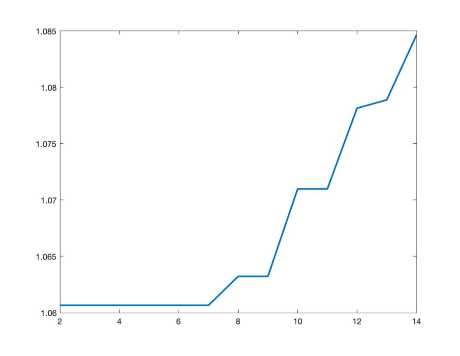
Figure 1. Growth of dual constant with $n$.

12. Computer experiment for finding $C_{dual}$

Let us consider the quantity

(12.1) $$C_{dual,n}:=\sup_{\|g\|_{L^{\infty}(\{-1,1\}^{n})}\leq 1}\|\int_{0}^{\infty}\nabla P_{t}g\,dt\|_{\infty}\,,$$

and let us try to find its numerical values for small dimensions $n$.

For $n=2$ the optimizer is

$$g(x_{1},x_{2})=\min(x_{1},x_{2})=(x_{1}x_{2}+x_{1}+x_{2}-1)/2.$$

In dimensions $n=3,\dots,7$, the optimal value is the same so one can just take two-dimensional function like $g(x_{1},\dots,x_{n})=\min(x_{1},x_{2}$). Of course, there may be many other optimizers.

The first nontrivial dimension where the $2D$ case is not optimal is $n=8$.

We would like to call the attention of the reader that the graph we get is extremely curious. It seems up to dimension $7$, two-dimensional functions are optimal. Then suddenly in dimension $8$ there is enough structure to do better with a truly eight-dimensional function.

The optimal value increases only very slowly. If we assume it grows sort of linearly (no reason it should, just to assume it to make some guesses), then one would extrapolate from the plot that $C_{dual,n}$ would reach $\sqrt{\pi/2}$ only around dimension $n=60$. This means that there is probably little insight to be gained from the specific structure of low-dimensional optimizers. Also, it is very different than the usual experience, which is that universality phenomena (like CLT) often kick in at surprisingly low dimension. For example, for Bernoulli $\varepsilon_{k}$ one has

$$\mathbb{E}|\varepsilon_{1}+...+\varepsilon_{9}|/\sqrt{9}|\approx 0.82,\,\,\mathbb{E}|\varepsilon_{1}+...+\varepsilon_{13}|/\sqrt{13}|\approx 0.81,$$

which is quite close to the Gaussian limit $\sqrt{2/\pi}\approx 0.80$. Here, we are very far from the Gaussian case and seem to approach it only very slowly.

See Fig. 1 for the growth of the dual constant with $n$. One can see that it grows very slowly (and does not grow at all for $n=2,\dots,7$). Then it slowly starts to pick up. Since we work with matrices of size $n\times 2^{n}$, their size grows too fast. We have already noted that the growth on this figure suggests that we come close to $\sqrt{\pi/2}$ only for $n=60$ or $70$. This experiment is beyond the computer reach.

13. $Curl$ space and $C_{dual}$

Let us remind the reader that

$$(f-\mathbb{E}f,g)=-(\nabla f,\int_{0}^{\infty}\nabla P_{t}g\,dt)\,.$$

Therefore,

$$\mathbb{E}|f-\mathbb{E}f|\leq\|\nabla f\|_{1}\cdot\sup_{\|g\|_{\infty}\leq 1}\Big{\|}\int_{0}^{\infty}\nabla P_{t}g\,dt\Big{\|}_{L^{\infty}/Curl}\leq$$

So we need to estimate

(13.1) $$C_{1}:=\sup_{\|g\|_{\infty}\leq 1}\inf_{h\in Curl}\|h+\int_{0}^{\infty}\nabla P_{t}g\,dt\|_{\infty}\,,$$

where the “$Curl$” space is the following:

$$Curl:=\{h=(h_{1},\dots,h_{n}):\mathbb{E}(h\cdot\nabla\varphi)=0\,,\forall\varphi\}\,.$$

Since $\nabla=(\partial_{1},\dots,\partial_{n})$, and $\partial_{k}$ is the elimination of $x_{k}$ operator:

$$\partial_{k}\varphi=\frac{1}{2}(\varphi^{x_{k}\to 1}-\varphi^{x_{k}\to-1})\,.$$

Space $Curl$ consists of vector functions $h=(h_{1},\dots,h_{n})$, such that

(13.2) $$\partial^{*}_{1}h_{1}+\dots+\partial^{*}_{n}h_{n}=0\,.$$

Here

$$\partial^{*}_{k}\varphi=x_{k}\frac{1}{2}(\varphi^{x_{k}\to 1}+\varphi^{x_{k}\to-1})\,.$$

In other words, it is a creation operator, that is

$$\partial^{*}_{k}x^{S}=\begin{cases}x_{k}x^{S},\,\,\text{if}\,\,k\notin S,\\ 0,\,\,\,\,\,\,\,\,\,k\in S\,.\end{cases}$$

Space $Curl$ is very large, as the vector functions $h$ such that $\partial^{*}_{k}h_{k}=0,k=1,\dots,n,$ are in this space. And for that to hold, it is enough for each $h_{k}$ to be of the following form:

(13.3) $$h_{k}=x_{k}\partial_{k}H_{k}$$

with arbitrary $H_{k}$, $k=1,\dots,n$. In fact, space $Curl$ is much larger than that.

To get the value of $C_{1}$ is the same as to calculate the quantity in (13.1). In the previous sections we gave some estimates on a potentially bigger quantity $C_{dual}$, which is given by the following formula:

(13.4) $$C_{dual}:=\sup_{\|g\|_{\infty}\leq 1}\|\int_{0}^{\infty}\nabla P_{t}g\,dt\|_{\infty}\,,$$

13.1. $Curl$ space in gaussian setting does not matter

Consider functions in $L^{1}(\mathbb{R}^{1},\gamma_{1})$ orthogonal to all $\mathcal{D}:=\{f^{\prime}:f\in C_{0}^{\infty}(\mathbb{R}^{1})\}$. Then

$$\int hf^{\prime}d\gamma_{1}=0,\quad\forall f^{\prime}\in\mathcal{D}\,.$$

Therefore,

$$-\int h^{\prime}fd\gamma+\int xhfd\gamma_{1}=0,\quad\forall f\in C_{0}^{\infty}\,.$$

Hence

$$h^{\prime}=xh,\quad h=C\cdot e^{\frac{x^{2}}{2}}\,.$$

This does not belong to $L^{1}(\gamma)$ unless $C=0$. So only zero function is in $Curl$. So in gaussian setting the $Curl$ space is zero.

But in dimension $2$ and higher curl space unfortunately exists in gaussian setting. In fact, in $2D$ this space consists of vector functions $h=(h_{1},h_{2})\in L^{1}(\mathbb{R}^{2},\gamma_{2})$ such that

(13.5) $$(h_{1})_{x_{1}}+(h_{2})_{x_{2}}=x_{1}h_{1}+x_{2}h_{2}\,,$$

which has a solution $h_{1}=-x_{2},h_{2}=x_{1}$.

In gaussian space, however, we know that

(13.6) $$C_{1}=C_{dual}\,,$$

where these constants can be seen in (13.1) and (13.4) correspondingly – where $P_{t}$ should be understood as Ornstein–Uhlenbeck semi-group.

For $n=1$ this follows from the above mentioned fact that $Curl=0$ for $1D$ gaussian case. Now let $n>1$. Let $G$ be the function of one variable that almost give the supremum in

$$\sup_{\|g\|_{\infty}\leq 1}\|\int_{0}^{\infty}\nabla P_{t}g\,dt\|_{\infty}$$

for $n=1$. Whence,

$$\|\int_{0}^{\infty}\nabla P_{t}^{(1)}G\,dt\|_{\infty}=\|\int_{0}^{\infty}e^{-t}P_{t}^{(1)}\nabla G\,dt\|_{\infty}\approx\sqrt{\frac{\pi}{2}}\,.$$

Here $P_{t}^{(1)}$ is Ornstein–Uhlenbeck semi-group in $L^{1}(\mathbb{R}^{1},\gamma_{1})$. Since function $G=G(x_{1})$, we can understand the last inequality also with $P_{t}^{(n)}$ is Ornstein–Uhlenbeck semi-group in $L^{1}(\mathbb{R}^{n},\gamma_{n})$:

$$\|\int_{0}^{\infty}\nabla P_{t}^{(n)}G\,dt\|_{\infty}=\|\int_{0}^{\infty}e^{-t}P_{t}^{(n)}\nabla G\,dt\|_{\infty}\approx\sqrt{\frac{\pi}{2}}\,.$$

This is because $(P_{t}^{(n)}g)(x)=(P_{t}^{(1)}g)(x_{1})$ for $g$ depending only on $x_{1}$.

14. Combinatorial formulation of $C_{dual}$

Constant $C_{dual}$, given by $C_{dual}:=\sup_{\|g\|_{\infty}\leq 1}\|\int_{0}^{\infty}\nabla P_{t}g\,dt\|_{\infty}$ is just

$$C_{dual}=\|T\|_{L^{\infty}\to L^{\infty}}\,,$$

where $T$ is, e.g. from (11.1), that is, $T=\nabla\Delta^{-1}P_{0}$.

The norm $\|T\|_{L^{\infty}\to L^{\infty}}$ is the smallest constant $C$ in the following inequality:

$$\|\nabla\Delta^{-1}P_{0}f\|_{\infty}\leq C\|f\|_{\infty},$$

which can be written down as follows

$$\|\nabla\Delta^{-1}f_{0}\|_{\infty}\leq C\inf_{a}\|f_{0}+a{\bf 1}\|_{\infty}\,,$$

where $f_{0}$ runs over all functions on Hamming cube that have zero average. Such functions can be written down as $f_{0}=\Delta F$, so we plug this representation into the above formula. Notice that $\Delta^{-1}\Delta F=F-\mathbb{E}F$. So we are looking at the best constant $C$ in

$$\|\nabla F\|_{\infty}=\|\nabla(F-\mathbb{E}F)\|_{\infty}\leq C\inf_{a}\|\Delta F+a{\bf 1}\|_{\infty}\,.$$

Denote Hamming graph as $(V,E)$, where vertices are denoted by $i=1,\dots,2^{n}$.

Then the previous best constant squared, namely, $C^{2}$ (that, is $C_{dual}^{2}$) is the best constant in the following inequality with arbitrary real numbers $\{a_{i}\}_{i=1}^{2^{n}}$:

(14.1) $$\sup_{i\in V}\sum_{j:(i,j)\in E}(a_{i}-a_{j})^{2}\leq C^{2}\inf_{a\in\mathbb{R}}\sup_{i\in V}\Big{(}a+\sum_{j:(i,j)\in E}(a_{i}-a_{j})\Big{)}^{2}\,.$$

In particular, we have proved that with $\varepsilon>0$ and independent of $n$

(14.2) $$\sup_{i\in V}\sum_{j:(i,j)\in E}(a_{i}-a_{j})^{2}\leq\Big{(}\frac{\pi}{2}-\varepsilon\Big{)}^{2}\sup_{i\in V}\Big{(}\sum_{j:(i,j)\in E}(a_{i}-a_{j})\Big{)}^{2}\,.$$

15. Calculations with matrix $M$. An example when $Curl$ space is essential

Recall that we introduced in (11.10) the following $n\times 2^{n}$ matrix $M_{\rho}:=(m_{i,z}(\rho))_{i=1,\dots,n;\,z\in\{-1,1\}^{n}}$:

(15.1) $$m_{i,z}(\rho):=2^{-n}\frac{z_{i}-\rho}{1-\rho^{2}}(1+\rho)^{n-d(z)}(1-\rho)^{d(z)}\,,\quad i=1,\dots,n,z\in\{-1,1\}^{n}\,,\rho\in(0,1)\,.$$

We considered it as acting from $\ell^{\infty}_{2^{n}}$ to $\ell^{2}_{n}$.

Of course, matrix elements $m_{i,z}:=2^{-n}K_{i}(z,{\bf 1})$ are just $\int_{0}^{1}m_{i,z}(\rho)\,d\rho$. Again we considered it as acting from $\ell^{\infty}_{2^{n}}$ to $\ell^{2}_{n}$, and we know that the sharp dual constant in $L^{1}$-Poincaré inequality is the norm of this matrix as acting from $\ell^{\infty}_{2^{n}}$ to $\ell^{2}_{n}$.

The norm of the matrix $M=(m_{i,z})=\int_{0}^{1}M_{\rho}\,d\rho$ as the matrix acting from $\ell^{\infty}_{2^{n}}$ to $\ell^{2}_{n}$ is

(15.2) $$\max_{\lambda,\,\|\lambda\|_{\ell^{2}_{n}}\leq 1}\mathbb{E}_{z}\Big{|}\sum_{i=1}^{n}\lambda_{i}\int_{0}^{1}\frac{z_{i}-\rho}{1-\rho^{2}}(1+\rho)^{n-d(z)}(1-\rho)^{d(z)}\,d\rho\Big{|}$$

We know that it is less than $\frac{\pi}{2}-\varepsilon$, where $\varepsilon>0$ does not depend on $n$.

There is a “sister” problem, where $L^{1}$-Poincaré inequality is replaced by $L^{\infty}$ one. It cannot have the form $\|f-\mathbb{E}f\|_{\infty}\leq C\|\nabla f\|_{\infty}$ with constant independent of $n$. This is impossible, e.g. because inequality $a_{1}+\dots+a_{n}\leq C(a_{1}^{2}+\dots+a_{n}^{2})^{1/2}$ is false. However, if one changes the definition of the gradient, then the corresponding inequality becomes meaningful and important (see, e.g., [11] or [18].)

Denote $|\tilde{\nabla}f|(x)=\sum_{i=1}^{n}|\partial_{i}f(x)|$. Then one can ask, whether the following inequality holds and with what sharp constant independent of $n$:

(15.3) $$\|f-\mathbb{E}f\|_{\infty}\leq C_{\infty}\|\tilde{\nabla}f\|_{\infty}\,?$$

This is a combinatorial question about the diameter of Hamming cube with weighted lengths of edges. Namely, this is equivalent to asking (see [11]) what is the supremum of $L^{\infty}$ norms of functions $f$ having zero average on cube and such that

(15.4) $$|\tilde{\nabla}f(x)|\leq 1\quad\forall x\in\{-1,1\}^{n}\,.$$

Remark 15.1.

Condition (15.4) can be reformulated in purely combinatorial terms as follows (see [11]): every edge of the graph (=Hamming cube) is provided with its variable “length” $\ell(x,y)$, and

$$\sum_{y\sim x}\ell(x,y)\leq 2\quad\forall x\in\{-1,1\}^{n}\,.$$

One wants then to know what is the universal sharp estimate on the diameter of the cube?

This becomes the question about independent of $n$ sharp constant $C_{\infty}$ such that (15.3) holds. The reference [11] has a very nice reasoning of F. Petrov that proves the following:

$$C_{\infty}=2\,.$$

Notice that we can easily translate the estimate (15.3) into a certain fact about our matrix $M=(m_{i,z})=\int_{0}^{1}M_{\rho}\,d\rho$ defined in (11.8). In fact, repeating our reasoning in the previous sections, we can notice that (15.3) is equivalent to finding

$$\sup_{f:\|f||_{L^{1}(\{-1,1\}^{n}}\leq 1}\inf_{h\in Curl}\|h+\int_{0}^{\infty}\nabla P_{t}fdt\|_{L^{1}(\{-1,1\}^{n};\ell^{\infty}_{n})}\,.$$

If $Curl$ space would not play any role, that would mean that we are interested in

$$\sup_{f:\|f||_{L^{1}(\{-1,1\}^{n}}\leq 1}\|\int_{0}^{\infty}\nabla P_{t}fdt\|_{L^{1}(\{-1,1\}^{n};\ell^{\infty}_{n})}\,.$$

We can calculate this norm now. It is the norm of our familiar operator

$$f\to\int_{0}^{\infty}\nabla P_{t}fdt$$

as acting from $L^{1}(\{-1,1\}^{n},d\mu)$ to $L^{1}(\{-1,1\}^{n},d\mu;\ell^{\infty}_{n})$.

This is the same the norm of operator $K=(K_{1},\dots,K_{n})$ (introduced in Section 11) as acting from $L^{1}(C^{n},d\mu)$ to $L^{1}(C^{n},d\mu;\ell^{\infty}_{n})$. Kernel $K_{i}(x^{\prime},x)$ can be written down as $K_{i}(x^{\prime},x)=x_{i}\tilde{K}_{i}(x^{\prime},x)$, where

$$\tilde{K}_{i}(x^{\prime},x):=\int_{0}^{\infty}e^{-t}x_{i}^{\prime}x_{i}\,\Pi_{k\neq i}^{n}(1+e^{-t}x_{k}^{\prime}x_{k})\,dt,$$

and we see that this is a kernel of the form $k_{i}(x^{\prime}\cdot x_{i})$, that is, it is a convolution kernel.

We use it with measure $d\mu(x^{\prime})$ that is invariant, meaning that $d\mu(x^{\prime}\cdot x)$ is the same measure. Notice also that the facts that $K_{i}(x^{\prime},x)=x_{i}\tilde{K}_{i}(x^{\prime},x),x_{i}=\pm 1,$ imply that the norm of operator with kernel $K$ is the same as the norm of operator with kernel $\tilde{K}$ – we mean here the action from $L^{1}(C^{n})\to L^{1}(C^{n};\ell^{\infty}_{n})$.

The norm of convolution operator from $L^{1}$ to $L^{1}$ is just $L^{1}$ norm of its kernel.

The reasoning that we have just made implies that the norm of the integral operator $K$ from $L^{1}(C^{n})\to L^{1}(C^{n};\ell^{\infty}_{n})$ is the same as the norm of the matrix $M:=(m_{i,z})_{i=1,\dots,n;\,z\in\{-1,1\}^{n}}$ considered as the vector function in $L^{1}(C^{n};\ell^{\infty}_{n})$, which is

$$\int_{C^{n}}\max_{i=1,\dots,n}|\tilde{K}_{i}(z,{\bf 1})d\mu(z)=\int_{C^{n}}\max_{i=1,\dots,n}|K_{i}(z,{\bf 1})d\mu(z)=\sum_{z\in C^{n}}\max_{i=1,\dots,n}|m_{i,z}|\,.$$

Matrix elements $m_{i,z}$ were computed in Section 11, see (11.8). So it is easy to calculate the latter quantity.

Formula (11.8) gives us the following:

• if $d(z)=\operatorname{dist}(z,{\bf 1})=0$, then for all $i$ we have $m_{i,z}(\rho)=2^{-n}(1+\rho)^{n-1}$,

• if $d(z)=\operatorname{dist}(z,{\bf 1})=1$, then $\max_{i=1,\dots,n}|m_{i,z}|=2^{-n}\int_{0}^{1}(1+\rho)^{n-1}d\rho$ again,

• if $d(z)=\operatorname{dist}(z,{\bf 1})=2$, then $\max_{i=1,\dots,n}|m_{i,z}|=2^{-n}\int_{0}^{1}(1+\rho)^{n-2}(1-\rho)d\rho$, …,

• if $d(z)=\operatorname{dist}(z,{\bf 1})=n$, then $\max_{i=1,\dots,n}|m_{i,z}|=2^{-n}\int_{0}^{1}(1-\rho)^{n-1}d\rho$.

Hence

$$\sum_{z\in C^{n}}\max_{i=1,\dots,n}|m_{i,z}|=2^{-n}\int_{0}^{1}[(1+\rho)^{n-1}+n(1+\rho)^{n-1}+\frac{n(n-1)}{2}(1+\rho)^{n-2}(1-\rho)+$$

$$\dots+(1-\rho)^{n-1}]\,d\rho=2^{-n}\int_{0}^{1}[n(1+\rho)^{n-1}+\frac{n(n-1)}{2}(1+\rho)^{n-2}(1-\rho)+\dots+(1-\rho)^{n-1}]\frac{1-\rho}{1-\rho}\,d\rho+$$

$$+2^{-n}\int_{0}^{1}(1+\rho)^{n-1}d\rho=$$

$$2^{-n}\int_{0}^{1}\frac{[(1+\rho)^{n}+n(1+\rho)^{n-1}(1-\rho)+\frac{n(n-1)}{2}(1+\rho)^{n-2}(1-\rho)^{2}+\dots+(1-\rho)^{n}-(1+\rho)^{n}]}{1-\rho}\,d\rho+$$

$$+2^{-n}\int_{0}^{1}(1+\rho)^{n-1}d\rho=$$

$$2^{-n}\int_{0}^{1}\frac{(1+\rho+1-\rho)^{n}-(1+\rho)^{n}}{1-\rho}\,d\rho+2^{-n}\int_{0}^{1}(1+\rho)^{n-1}d\rho=\int_{0}^{1}\frac{1-(\frac{1+\rho}{2})^{n}}{1-\rho}\,d\rho+\frac{2^{-n}}{n}(2^{n}-1)=$$

$$2\int_{1/2}^{1}\frac{1-x^{n}}{2(1-x)}\,dx+O\big{(}\frac{1}{n}\big{)}=\int_{1/2}^{1}(1+x+x^{2}+\dots x^{n-1})\,dx+O\big{(}\frac{1}{n}\big{)}=1+\frac{1}{2}+\frac{1}{3}+\dots+\frac{1}{n}+O(1)=$$

$$\log n+O(1)\,.$$

We see that the operator norm $\sup_{f:\|f||_{L^{1}(\{-1,1\}^{n}}\leq 1}\|\int_{0}^{\infty}\nabla P_{t}fdt\|_{L^{1}(\{-1,1\}^{n};\ell^{\infty}_{n})}$ grows logarithmically with $n$. So $Curl$ space plays major part for the calculation of $C_{\infty}$ since we know from [11], [18] that $C_{\infty}$ is bounded independent of $n$. One cannot forget about $Curl$ space in this problem.

16. Some formulas for $C_{dual}$

As we know

(16.1) $$C_{dual}=\lim_{n\to\infty}\sup_{\|v\|_{\ell_{n}^{2}}\leq 1}\mathbb{E}_{z}\Big{|}\sum_{i=1}^{n}v_{i}\int_{0}^{1}\frac{z_{i}-\rho}{1-\rho^{2}}(1+\rho)^{n-d({\bf 1},z)}(1-\rho)^{d({\bf 1},z)}\,d\rho\Big{|}$$

Let $B(a,b)=\int_{0}^{1}t^{a-1}(1-t)^{b-1}$ denote the beta function. For $k=d({\bf 1},z)$ integrals

$$2^{-n}\int_{0}^{1}\frac{z_{i}-\rho}{1-\rho^{2}}(1+\rho)^{n-d({\bf 1},z)}(1-\rho)^{d({\bf 1},z)}\,d\rho=\begin{cases}\int_{0}^{1/2}t^{k}(1-t)^{n-k-1}dt,\quad z_{i}=1\\ -\int_{0}^{1/2}t^{k-1}(1-t)^{n-k}dt,\quad z_{i}=-1\end{cases}$$

are certain combinatorial quantities called “incomplete beta functions”

$$=\begin{cases}B_{1/2}(k+1,n-k)=F_{1/2}(n-k-1,n)\cdot B(k+1,n-k),\quad\text{if}\,\,z_{i}=1,\\ B_{1/2}(k,n-k+1)=-F_{1/2}(n-k,n)\cdot B(k,n-k+1),\quad\text{if}\,\,z_{i}=-1\,.\end{cases}$$

This can be written down as

$$=\begin{cases}B_{1/2}(k+1,n-k)=F_{1/2}(n-k-1,n)\frac{1}{(n-k)\binom{n}{k}},\quad\text{if}\,\,z_{i}=1,\\ B_{1/2}(k,n-k+1)=-F_{1/2}(n-k,n)\frac{1}{k\binom{n}{k}},\quad\text{if}\,\,z_{i}=-1\,.\end{cases}$$

Here $F_{1/2}(n-k-1,n)$ is the probability of at least $k+1$ successes in Bernoulli scheme with $n$ trials:

$$F_{1/2}(n-k-1,n)=2^{-n}\sum_{r=k+1}^{n}\binom{n}{r}\,.$$

Thus, we can rewrite the main part of formula (16.1) for $C_{dual}$ as follows

$$\mathbb{E}_{z}\Big{|}\sum_{i=1}^{n}v_{i}\int_{0}^{1}\frac{z_{i}-\rho}{1-\rho^{2}}(1+\rho)^{n-d({\bf 1},z)}(1-\rho)^{d({\bf 1},z)}\,d\rho\Big{|}=$$

$$=\frac{1}{2^{n}}\sum_{k=0}^{n}\binom{n}{k}\mathbb{E}\Big{[}\Big{|}\sum_{i=1}^{n}v_{i}\frac{1}{\binom{n}{k}}\frac{2z_{i}}{1+(1-2k/n)z_{i}}\sum_{r=k+1-1_{z_{i}=-1}}^{n}\binom{n}{r}\Big{|}\Big{|}d({\bf 1},z)=k\Big{]}$$

$$=\frac{1}{2^{n}}\sum_{k=0}^{n}\mathbb{E}\Big{[}\Big{|}\sum_{i=1}^{n}v_{i}\frac{2z_{i}}{1+(1-2k/n)z_{i}}\sum_{r=k+1-1_{z_{i}=-1}}^{n}\binom{n}{r}\Big{|}\Big{|}d({\bf 1},z)=k\Big{]}$$

$$=\frac{1}{n2^{n-1}}\sum_{k=0}^{n-1}\sum_{r=k+1}^{n}\binom{n}{r}\mathbb{E}\Big{[}\Big{|}\sum_{i=1}^{n}v_{i}\frac{z_{i}}{1+(1-2k/n)z_{i}}\Big{|}\Big{|}d({\bf 1},z)=k\Big{]}$$

$$+\frac{1}{2^{n}}\sum_{k=1}^{n}\frac{1}{k}\binom{n}{k}\mathbb{E}\Big{[}\Big{|}\sum_{i:\,z_{i}=-1}v_{i}\Big{|}\Big{|}d({\bf 1},z)=k\Big{]}$$

But $\|v\|_{2}\leq 1$, so $\mathbb{E}\Big{[}\Big{|}\sum_{i:\,z_{i}=-1}v_{i}\Big{|}\Big{|}d({\bf 1},z)=k\Big{]}\leq\sqrt{k}$. Therefore, the last sum is

$$\leq\frac{1}{2^{n}}\sum_{k=1}^{n}\frac{1}{\sqrt{k}}\binom{n}{k}\leq\sqrt{\frac{1}{2^{n}}\sum_{k=1}^{n}\frac{1}{k}\binom{n}{k}}\leq\frac{2}{\sqrt{n+1}}\to 0.$$

Hence, we can rewrite

$$\mathbb{E}_{z}\Big{|}\sum_{i=1}^{n-1}v_{i}\int_{0}^{1}\frac{z_{i}-\rho}{1-\rho^{2}}(1+\rho)^{n-d({\bf 1},z)}(1-\rho)^{d({\bf 1},z)}\,d\rho\Big{|}=$$

$$\frac{1}{n2^{n-1}}\sum_{k=0}^{n}\sum_{r=k+1}^{n}\binom{n}{r}\mathbb{E}\Big{[}\Big{|}\sum_{i=1}^{n}v_{i}\frac{z_{i}}{1+(1-2k/n)z_{i}}\Big{|}\Big{|}d({\bf 1},z)=k\Big{]}+o(1)\,.$$

Here is the first formula for $C_{dual}$:

(16.2) $$C_{dual}=\lim_{n\to\infty}\sup_{\|v\|_{\ell_{n}^{2}}\leq 1}\frac{1}{n2^{n-1}}\sum_{k=0}^{n-1}\sum_{r=k+1}^{n}\binom{n}{r}\mathbb{E}\Big{[}\Big{|}\sum_{i=1}^{n}v_{i}\frac{z_{i}}{1+(1-2k/n)z_{i}}\Big{|}\Big{|}d({\bf 1},z)=k\Big{]}\,.$$

We can simplify further this formula. For that, consider

$$\Phi_{n}(k):=\frac{1}{2^{n}}\sum_{r=k+1}^{n}\binom{n}{r}=\mathbb{P}[\text{Binom}(n,\frac{1}{2})>k]\,.$$

This implies

$$\Phi_{n}(\frac{\sqrt{n}}{2}+\frac{x\sqrt{n}}{2})\to\mathbb{P}[N(0,1)>x]\,.$$

Theorem 16.1.

(16.3) $$C_{dual}=\lim_{n\to\infty}\sup_{\|v\|_{\ell_{n}^{2}}\leq 1}\frac{2}{n}\sum_{k=0}^{n/2}\mathbb{E}\Big{[}\Big{|}\sum_{i=1}^{n}v_{i}\frac{z_{i}}{1+(1-2k/n)z_{i}}\Big{|}\Big{|}d({\bf 1},z)=k\Big{]}\,.$$

Proof.

Define

$$X_{i}^{k}:=\frac{z_{i}}{1+(1-2k/n)z_{i}}\,.$$

By Cauchy–Schwarz we get

(16.4) $$\mathbb{E}[\sum_{i=1}^{n}v_{i}X_{i}^{k}|d({\bf 1},z)=k]\leq\sum_{i,j=1}^{n}v_{i}v_{j}\mathbb{E}[X_{j}^{k}X_{i}^{k}|d({\bf 1},z)=k]\,.$$

It is easy to see that

$$\mathbb{E}[X_{i}^{k}|d({\bf 1},z)=k]=0,$$

$$\mathbb{E}[(X_{i}^{k})^{2}|d({\bf 1},z)=k]=\frac{n^{2}}{4k(n-k)},$$

$$\mathbb{E}[X_{i}^{k}X_{j}^{k}|d({\bf 1},z)=k]=-\frac{1}{n-1}\frac{n^{2}}{4k(n-k)},\quad i\neq j.$$

Hence, we know the Gramm matrix $G:=\{\mathbb{E}[X_{j}^{k}X_{i}^{k}|d({\bf 1},z)=k]\}$. It is self adjoint rank one perturbation of the diagonal matrix $\text{diag}(\frac{n}{n-1}\frac{n^{2}}{4k(n-k)})$. So it is easy to calculate the norm of $G$. It is $\sqrt{\frac{n}{n-1}\frac{n^{2}}{4k(n-k)}}$.

Hence, by (16.4)

(16.5) $$\mathbb{E}[\sum_{i=1}^{n}v_{i}X_{i}^{k}|d({\bf 1},z)=k]\leq\sqrt{\frac{n}{n-1}\frac{n^{2}}{4k(n-k)}}\,.$$

Let $b_{n}=\sqrt{n}\log n$. By the same spectral estimate for a cut-off matrix and by the fact that $\Phi_{n}(k)\leq 1$, we will get

(16.6) $$\sum_{k=n/2-b_{n}}^{n/2+b_{n}}\Phi_{n}(k)\mathbb{E}[\sum_{i=1}^{n}v_{i}X_{i}^{k}|d({\bf 1},z)=k]\leq\sum_{k=n/2-b_{n}}^{n/2+b_{n}}\sqrt{\frac{n}{n-1}\frac{n^{2}}{4k(n-k)}}=O(b_{n})\,.$$

Thus,

(16.7) $$\frac{1}{n2^{n-1}}\sum_{k=n/2-b_{n}}^{n/2+b_{n}}\sum_{r=k+1}^{n}\binom{n}{r}\mathbb{E}\Big{[}\Big{|}\sum_{i=1}^{n}v_{i}\frac{z_{i}}{1+(1-2k/n)z_{i}}\Big{|}\Big{|}d({\bf 1},z)=k\Big{]}=O\big{(}\frac{\log n}{\sqrt{n}}\big{)}\,.$$

Using the spectral estimate for another cut-off matrix and the fact that $\sqrt{\frac{n}{n-1}\frac{n^{2}}{4k(n-k)}}=O(\sqrt{n})$, we get

(16.8) $$\mathbb{E}[\sum_{i=1}^{n}v_{i}X_{i}^{k}|d({\bf 1},z)=k]\leq\sqrt{\frac{n}{n-1}\frac{n^{2}}{4k(n-k)}}=O(\sqrt{n})\,.$$

Hence,

$$\sum_{k=n/2+b_{n}}^{n-1}\Phi_{n}(k)\mathbb{E}\Big{[}\Big{|}\sum_{i=1}^{n}v_{i}\frac{z_{i}}{1+(1-2k/n)z_{i}}\Big{|}\Big{|}d({\bf 1},z)=k\Big{]}=O\Big{(}\sqrt{n}\sum_{k=n/2+b_{n}}^{n-1}\Phi_{n}(k)\Big{)}$$

(16.9) $$=O(n^{3/2}\Phi_{n}(n/2+b_{n}))=O(n^{3/2}e^{-\log^{2}n})\,.$$

(16.10) $$\frac{1}{n2^{n-1}}\sum_{k=n/2+b_{n}}^{n-1}\sum_{r=k+1}^{n}\binom{n}{r}\mathbb{E}\Big{[}\Big{|}\sum_{i=1}^{n}v_{i}\frac{z_{i}}{1+(1-2k/n)z_{i}}\Big{|}\Big{|}d({\bf 1},z)=k\Big{]}=O\big{(}n^{1/2}e^{-\log^{2}n}\big{)}\,.$$

So when we come to the limit with $n\to\infty$ in (16.2), we are left with

$$C_{dual}=\lim_{n\to\infty}\sup_{\|v\|_{\ell_{n}^{2}}\leq 1}\frac{1}{n2^{n-1}}\sum_{k=n/2-b_{n}}^{n-1}\sum_{r=k+1}^{n}\binom{n}{r}\mathbb{E}\Big{[}\Big{|}\sum_{i=1}^{n}v_{i}\frac{z_{i}}{1+(1-2k/n)z_{i}}\Big{|}\Big{|}d({\bf 1},z)=k\Big{]}=$$

$$=\lim_{n\to\infty}\sup_{\|v\|_{\ell_{n}^{2}}\leq 1}\frac{2}{n}\sum_{k=n/2-b_{n}}^{n-1}\Phi_{n}(k)\mathbb{E}\Big{[}\Big{|}\sum_{i=1}^{n}v_{i}\frac{z_{i}}{1+(1-2k/n)z_{i}}\Big{|}\Big{|}d({\bf 1},z)=k\Big{]}=$$

$$=\lim_{n\to\infty}\sup_{\|v\|_{\ell_{n}^{2}}\leq 1}\frac{2}{n}\sum_{k=n/2-b_{n}}^{n-1}\mathbb{E}\Big{[}\Big{|}\sum_{i=1}^{n}v_{i}\frac{z_{i}}{1+(1-2k/n)z_{i}}\Big{|}\Big{|}d({\bf 1},z)=k\Big{]},$$

the last equality being true because in this range of $k$ we have

$$1-O(e^{-\log^{2}n})\leq\Phi_{n}(k)\leq 1\,.$$

Now we can add back

$$\frac{2}{n}\sum_{k=n/2-b_{n}}^{n/2+b_{n}}\mathbb{E}\Big{[}\Big{|}\sum_{i=1}^{n}v_{i}\frac{z_{i}}{1+(1-2k/n)z_{i}}\Big{|}\Big{|}d({\bf 1},z)=k\Big{]}$$

and

$$\frac{2}{n}\sum_{k=n/2+b_{n}}^{n-1}\mathbb{E}\Big{[}\Big{|}\sum_{i=1}^{n}v_{i}\frac{z_{i}}{1+(1-2k/n)z_{i}}\Big{|}\Big{|}d({\bf 1},z)=k\Big{]}$$

as we already saw that they are $O\big{(}\frac{\log n}{\sqrt{n}}\big{)}$ and $O\big{(}e^{-\log^{2}n}\big{)}$ correspondingly. Theorem is completely proved. ∎

Remark 16.2.

From (16.5) and (16.2) one immediately deduces the estimate

(16.11) $$C_{dual}\leq\lim_{n\to\infty}\sum_{k=1}^{n-1}\Phi_{n}(k)\frac{1}{\sqrt{k(n-k)}}=\frac{\pi}{2}\,.$$

Of course Theorem 16.1 also immediately gives this estimate. This is one of the numerous re-proofs of Lust-Piquard–Ben Efraim estimate from [1]. As we can see the reason for their estimate lies in Cauchy–Schwarz estimate and spectral calculation for the Gramm matrix.

Remark 16.3.

What we did in this paper, was that we estimated by funny Khintchine inequality another (and formally bigger than $C_{dual}$) quantity

(16.12) $$\lim_{n\to\infty}\int_{0}^{1}\sup_{\|v\|_{\ell_{n}^{2}}\leq 1}\mathbb{E}_{z}\Big{|}\sum_{i=1}^{n}v_{i}\frac{z_{i}-\rho}{1-\rho^{2}}\Big{|}(1+\rho)^{n-d({\bf 1},z)}(1-\rho)^{d({\bf 1},z)}\,d\rho<\frac{\pi}{2}\,.$$

References

[1]L. Ben Efraim, F. Lust-Piquard, Poincaré type inequalities on the discrete cube and in the CAR algebra,
Probab. Theory Related Fields 141 (2008), no. 3-4, 569–602.
[2]D. Bakry, I. Gentil, M. Ledoux, Analysis and Geometry of Markov Diffusion Operator, Grundlehren der mathematischen Wissenschaften, v. 348, Springer, 2014.
[3]Sergey G. Bobkov, Gennadiy P. Chistyakov, On Concentration Functions of Random Variables, J. Theor. Probab.
DOI 10.1007/s10959-013-0504-1.
[4]S.G. Bobkov, An isoperimetric inequality on the discrete cube, and an elementary proof of the isoperimetric inequality in Gauss space, The Annals of Probability
1997, Vol. 25, No. 1, 206–214.
[5]S.G. Bobkov, F. Gotze, Exponential integrability and transportation cost related to logarithmic Sobolev inequalities,
J. Funct. Anal. 163 (1) (1999) 1–28.
[6]Dong Li, On a frequency localized Bernstein inequality and some generalized Poincaré-type inequalities,
Math. Res. Lett. 20 (2013), no. 5, 933–945.
[8]Paata Ivanisvili, Fedor Nazarov and Alexander Volberg,
Square function and the Hamming cube: Duality, to appear in Discrete Analysis, 2018.
[9]Paata Ivanisvili, Alexander Volberg, Isoperimetric functional inequalities via the maximum principle: the exterior differential systems approach, arxiv. 1511.06895,
Operator Theory:
Advances and Applications, Vol. 261, 279–303, Birkhauser volume dedicated to V. P. Khavin.
[10]R. O’Donnell, Analysis of Boolean functions, Cambridge University Press, 2014.
[11]P. Ivanisvili, B. Kloeckner, F. Nazarov, F. Petrov, https://mathoverflow.net/questions/286329/diameter-of-a-weighted-hamming-cube/303016-303016
[12]G. Pisier, Probabilistic methods in the geometry of Banach spaces, in: Probability and Analysis, (Varenna, 1985), Lecture Notes in Math. 1206, Springer, Berlin, 1986.
[13]G. Samorodnitsky, M. Taqqu, Stable non-Gaussian Random Processes. Chapman and Hall, New York, London, 1994, 632 pp.
[14]A. Naor, T. Hytönen, Pisier’s inequality revisited, Studia Mathematica 215 (2013), no. 3, 221–235.
[15]Y. Shenfeld, R. van Handel , The equality cases of the Ehrhard-Borell inequality. Adv. Math. 331 (2018), 339–386.
[16]M. Talagrand, Isoperimetry, logarithmic Sobolev inequalities on the discrete cube, and Margulis’ graph connectivity theorem, Geometric and Functional Analysis (GAFA), 3 (1993), No. 3, pp. 295–314.
[17]R. van Handel, The Borell–Ehrhard game. Probab. Theory Related Fields 170 (2018), no. 3–4, 555–585.
[18]R. Wagner, Notes on an inequality by Pisier for functions on the discrete cube, Milman, V. D. (ed.) et al., Geometric aspects of functional analysis. Proceedings of the Israel seminar (GAFA) 1996-2000. Berlin: Springer. Lect. Notes Math. 1745, 263-268 (2000).