Number of Particles in Fission Fragments

Abstract

Background

In current simulations of fission, the number of protons and neutrons in a given fission fragment is almost always obtained by integrating the total density of particles in the sector of space that contains the fragment. The semiclassical nature of this procedure and the antisymmetry of the many-body wave-function of the whole nucleus systematically leads to noninteger numbers of particles in the fragment.

Purpose

We seek to estimate rigorously the probability of finding $Z$ protons and $N$ neutrons in a fission fragment, i.e., the dispersion in particle number (both charge and mass). Knowing the dispersion for any possible fragmentation of the fissioning nucleus will improve the accuracy of predictions of fission fragment distributions and the simulation of the fission spectrum with reaction models.

Methods

Given a partition of the full space $\mathbb{R}^{3}$ in two sectors corresponding to the two prefragments, we discuss two different methods. The first one is based on standard projection techniques extended to arbitrary partitions of space. We also introduce a novel sampling method that depends only on a relevant single-particle basis for the whole nucleus and the occupation probability of each basis function in each of the two sectors. We estimate the number of particles $A$ in the left (right) fragment by statistical sampling of the joint probability of having $A$ single-particle states in the left (right) sector of space.

Results

We use both methods to estimate the charge and mass number dispersion of several scission configurations in ²⁴⁰Pu using either a macroscopic-microscopic approach or full Hartree-Fock-Bogoliubov calculations. We show that restoring particle-number symmetry naturally produces odd-even effects in the charge probability, which could explain the well-known odd-even staggering effects of charge distributions.

Conclusions

We discuss two methods to estimate particle-number dispersion in fission fragments. In the limit of well-separated fragments, the two methods give identical results. It can then be advantageous to use the sampling method since it provides a $N$-body basis for each prefragment, which can be used to estimate fragment properties at scission. When the two fragments are still substantially entangled, the sampling method breaks down and one has to use projector techniques, which gives the exact particle-number dispersion even in that limit. Note that in this paper, we have assumed that scission configurations could be described well by a static Bogoliubov vacuum: the strong odd-even staggering in the charge distributions could be somewhat attenuated when going beyond this hypothesis.

I Introduction

The theoretical understanding of nuclear fission, discovered in 1938 by O. Hahn and F. Strassmann, remains a vexing challenge even to this day. The fission of a heavy atomic nucleus presents a number of conceptual as well as practical difficulties. A fissioning nucleus is a particular example of a quantum many-body system of strongly interacting fermions, whose interaction is only known approximately. Fission dynamics is explicitly time dependent and involves open channels (mostly neutrons, but also photons). From a fundamental perspective, the physics of scission, or how an interacting, quantum many-body system splits into two well-separated interacting quantum many-body systems is very poorly known. Although there has been a considerable body of experimental work on fission in general, the most accurate data involve the decay of the fission fragments. The mechanism by which these fragments are formed in the first place must be described by theory.

Several approaches have been developed over the years to describe the fission process. Since fission times are rather slow compared with single-particle (s.p.) types of excitations Bulgac et al. (2016, 2018), quasistatic approaches are well justified. Most incarnations of these approaches rely on identifying a few collective variables that drive the fission process, mapping out the potential energy surface in this collective space (which fixes all properties of fission fragments) and computing the probability for the nucleus to be at any point on the surface, e.g., with semiclassical dynamics, such as Langevin  Abe et al. (1996); Fröbrich and Gontchar (1998); Usang et al. (2016), random walk Randrup et al. (2011); Randrup and Möller (2011, 2013); Ward et al. (2017) or with fully quantum-mechanical dynamics such as the time-dependent generator coordinate method Berger et al. (1984); Goutte et al. (2005); Regnier et al. (2016, 2018). One major limitation of these approaches is the need to identify scission configurations in the potential energy surface, that is, the arbitrary frontier that separates configurations where the nucleus is whole from those where it has split into two fragments Younes and Gogny (2011); Schunck et al. (2014); Schunck and Robledo (2016). In practice, such scission configurations happen to always be characterized by noninteger values of average particle numbers in the fragments.

The arbitrariness of the very concept of scission is strongly mitigated in explicitly nonadiabatic theories of fission, such as the various formulations of time-dependent nuclear density functional theory Umar et al. (2010); Simenel and Umar (2014); Goddard et al. (2015); Scamps et al. (2015); Tanimura et al. (2015); Bulgac et al. (2016); Goddard et al. (2016); Tanimura et al. (2017); Bulgac et al. (2018). Since these approaches simulate the real-time evolution of the nucleus and explicitly conserve energy, one can obtain excellent estimates of fission fragment properties well past the actual scission point Simenel and Umar (2014); Bulgac et al. (2016, 2018). However, these theories still simulate the evolution of the fissioning nucleus instead of the fragments themselves: The latter remain entangled even after scission and, thus, have also noninteger values of protons and neutrons Scamps et al. (2015). Particle-number symmetry in the fragments could, in principle, be restored by using standard projection techniques. This approach was pioneered initially in the case of particle transfer in heavy-ion fusion reactions Simenel (2010); Scamps and Lacroix (2013); Sekizawa and Yabana (2013, 2014). However, as we will discuss below, projection techniques do not allow to identify independent configurations in the fragments. Although this does not impact the estimate of primary charge or mass yields, it would be very useful to have access to a basis of $N$-body Slater determinants of particles to calculate other observables.

Our goal is, thus, to explore an alternative method to estimate the number of particles in the fission fragments. More precisely, given a description of the fissioning system by an $A$-body Slater determinant or a quasiparticle vacuum, we seek to determine both the probability that the total $N$-body wave-function contains a Slater determinant of particles with $A_{1}$ ($A_{2}$) particles in the left (right) fragment, both $A_{1}$ and $A_{2}$ being integers and $A_{1}+A_{2}=A$, as well as a suitable basis of s.p. states to describe them. In this paper, we propose a new method that only depends on a physically relevant s.p. basis for the fissioning nucleus and a set of occupation probabilities.

We present our theoretical framework in Section II. This includes some general notations, the presentation of our Monte Carlo (MC) sampling method, and a reminder of projection techniques adapted to the case of fission fragments. Section III is focused on the validation and numerical implementation of the sampling method. In Section IV, we study in more details the fragmentation probabilities for scission configurations in ²⁴⁰Pu, before concluding in Section V.

II Theoretical Formalism

The prediction of the primary mass or charge distribution in fission can be decomposed in three steps Schunck and Robledo (2016). First, one calculates the energy of the fissioning system for a set of configurations with different geometric shapes or constraints. This potential energy surface (PES) is divided into two regions, one where the nucleus has split into two fragments, the other where it has not; scission configurations correspond to the frontier between the two regions. In a second step, one estimates the probability to populate each scission configuration. This can be done either semiclassically by solving the Langevin equation as in Refs. Nadtochy and Adeev (2005); Nadtochy et al. (2007); Sadhukhan and Pal (2011); Nadtochy et al. (2012); Aritomo et al. (2015); Sadhukhan et al. (2016); Usang et al. (2016); Ishizuka et al. (2017); Sierk (2017); Usang et al. (2017) or with a random walk approach Randrup et al. (2011); Randrup and Möller (2011, 2013); Möller and Ichikawa (2015); Ward et al. (2017), or more microscopically by using time-dependent configuration techniques, such as the time-dependent generator coordinate method with the Gaussian overlap approximation (TDGCM-GOA) Goutte et al. (2004, 2005); Regnier et al. (2016); Zdeb et al. (2017); Tao et al. (2017); Zhao et al. (2019); Regnier et al. (2019). Finally, the result of the time-dependent evolution are coupled with an estimate of fragment properties to estimate the actual distribution of nuclear observables, such as charge, mass, total kinetic energy (TKE), etc.

In the case of charge and mass distributions, the last step of the procedure outlined above involves estimating the particle number in the fission fragments. Until recently, all fission calculations have used a semiclassical estimate of the average particle number based on integrating the one-body density. Below, we describe two methods to obtain integer values of particle number. The first method, which is developed in this paper, involves a Monte Carlo sampling of s.p. configurations. Its main advantage is that it indirectly provides a set of s.p. wave-functions for each of the fragments, which could then be used to estimate quantities, such as, e.g., the level density. The second method is based on extending standard projection techniques to arbitrary space partitionings and was introduced originally by Simenel in Simenel (2010) for Slater determinants and later extended in Scamps and Lacroix (2013) to the case of superfluid systems.

II.1 Space partitioning

Let us first assume that the state $|{\Phi}\rangle$ of the fissioning system is a Slater determinant of particles,

$$|{\Phi}\rangle\equiv\prod_{k=0}^{A-1}\hat{c}^{{\dagger}}_{k}|{0}\rangle,$$ (1)

where $|{0}\rangle$ is the particle vacuum. The operator $\hat{c}^{{\dagger}}_{k}$ creates a fermion in the s.p. state $k$ and reads

$$\hat{c}^{{\dagger}}_{k}=\int_{\mathcal{V}}\mathrm{d}^{3}\bm{r}\,\varphi_{k}(\bm{r})\hat{c}^{{\dagger}}({\bm{r}}),$$ (2)

where $\varphi_{k}(\bm{r})$ is the s.p. wave-function for state $k$ and the operator $\hat{c}^{{\dagger}}({\bm{r}})$ creates a well-localized fermion at point $\bm{r}$ (we omit spin and isospin degrees of freedom for the sake of simplicity). Recall that the set of all functions $\varphi_{k}(\bm{r})$ forms a basis of the $\mathcal{L}_{2}$ Hilbert space of square-integrable functions.

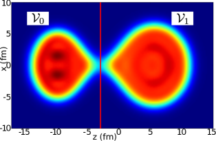
Figure 1: Illustration of the partition of the space $\mathcal{V}$ into $\mathcal{V}_{0}$ and $\mathcal{V}_{1}$ using the local density. The color scale corresponds to the value of the local density associated with a Slater determinant $|{\Phi}\rangle$. The red line separates $\mathcal{V}_{0}$ (to the left of the line) and $\mathcal{V}_{1}$ (to the right of the line).

We also assume that it is possible to partition the full space $\mathcal{V}\equiv\mathbb{R}^{3}$ into two sectors $\mathcal{V}_{0}$ and $\mathcal{V}_{1}$ such that $\mathcal{V}_{0}$ ($\mathcal{V}_{1}$) is the region where the left (right) fragment is localized. Such a partitioning could, for instance, be defined by introducing the coordinates of a neck between the two prefragments at scission as illustrated schematically in Figure 1. The two prefragments are separated by the red line located at the neck position. It is, then, always possible to decompose the s.p. wave-functions into

$$\varphi_{k}(\bm{r})=\alpha_{k}^{(0)}\varphi^{(0)}_{k}(\bm{r})+\alpha_{k}^{(1)}\varphi^{(1)}_{k}(\bm{r}),$$ (3)

where $\varphi^{(p)}_{k}(\bm{r})$ is defined in $\mathcal{V}_{p}$ ($p=0,1$) and $\alpha_{k}^{(p)}$ are normalization coefficients obtained by integrating the s.p. wave-functions in the domain $\mathcal{V}_{p}$,

$$\alpha_{k}^{(p)}=\sqrt{\int_{\mathcal{V}_{p}}d^{3}\bm{r}\,|\varphi_{k}(\bm{r})|^{2}}.$$ (4)

In terms of operators, the expansion of Eq.(3) simply translates into

$$\hat{c}^{{\dagger}}_{k}=\alpha_{k}^{(0)}\hat{c}^{(0){\dagger}}_{k}+\alpha_{k}^{(1)}\hat{c}^{(1){\dagger}}_{k}.$$ (5)

The ladder operators $\hat{c}^{(0){\dagger}}_{k}$, $\hat{c}^{(1){\dagger}}_{k}$ and their Hermitian conjugates verify the following anticommutation relations ($p,r=0,1$)

$$\left\{\hat{c}^{(p){\dagger}}_{k},\hat{c}^{(r){\dagger}}_{l}\right\} =\left\{\hat{c}^{(p)}_{k},\hat{c}^{(r)}_{l}\right\}=0$$ (6)

$$\left\{\hat{c}^{(p){\dagger}}_{k},\hat{c}^{(r)}_{l}\right\} =\delta_{pr}\int{\rm d}\bm{r}\ \varphi^{(p)}_{k}(\bm{r})\varphi^{(r)*}_{l}(\bm{r})$$ (7)

In the general case, $\{\hat{c}^{(p){\dagger}}_{k},\hat{c}^{(p)}_{l}\}\neq 0$ when $k\neq l$. However, it is always possible to restore all the fermion anticommutation relations by orthonormalizing (for example with the Gram-Schmidt procedure) the bases $\{\hat{c}^{(0){\dagger}}_{k}\}$ and $\{\hat{c}^{(1){\dagger}}_{k}\}$ separately. Given these prerequisites, the goal of our method is to estimate the relative probability of finding a many-body state with $N_{p}$ particles in the subspace $\mathcal{V}_{p}$.

II.2 Monte Carlo Approach

We first present a method that only requires the coefficients (4). Calculating them requires, in turn, only two ingredients: a set of s.p. wave-functions and a partitioning of $\mathbb{R}^{3}$. Let us emphasize that from a mathematical or algorithmic point of view, the partitioning of the space is entirely arbitrary. We refer to our method as MC sampling.

II.2.1 Orthonormal Bases

We first introduce the general principles of our method for the idealized case where the $\varphi_{k}^{(p)}$ form an orthonormal basis of $\mathcal{V}_{p}$. We emphasize very clearly that, in the most general case, this condition is not satisfied. In the context of fission, however, it can be approached asymptotically in the limit of infinitely separated fragments. In practice, it is reasonable to assume that scission configurations will sufficiently well approximate this limiting case so that the method can still provide reasonable estimates of the particle numbers.

If the $\varphi_{k}^{(p)}$ form an orthonormal basis of $\mathcal{V}_{p}$, then the fermion anticommutation relations between the corresponding s.p. operators are satisfied. Let us insert Eq. (5) in Eq. (1). We obtain

$$|{\Phi}\rangle=\sum_{\begin{subarray}{c}\bm{p}=(p_{0},\dots,p_{A-1})\\ p_{k}\in(0,1)\end{subarray}}\left[\prod_{k=0}^{A-1}\alpha_{k}^{(p_{k})}\right]\left[\prod_{k=0}^{A-1}\hat{c}^{(p_{k}){\dagger}}_{k}\right]|{0}\rangle.$$ (8)

In Eq. (8), we sum over all possible $A$-uplets of $0$ and $1$. Since we assume that the $\hat{c}^{(0){\dagger}}_{k}$ and $\hat{c}^{(1){\dagger}}_{k}$ correspond to orthonormal bases, the $A$-body state $|{\bm{p}}\rangle$ defined by

$$|{\bm{p}}\rangle=\prod_{k=0}^{A-1}\hat{c}^{(p_{k}){\dagger}}_{k}|{0}\rangle$$ (9)

is a Slater determinant. By using the fermion anticommutation relations of the $\hat{c}^{(p){\dagger}}_{k}$, we see that the set of all the possible $|{\bm{p}}\rangle$ forms an orthonormal basis of the $A$-body space. By construction, each state $|{\bm{p}}\rangle$ is an eigenvector of the particle-number operators for both $\mathcal{V}_{0}$ and $\mathcal{V}_{1}$ and contains two sets of particles. The first set is completely in $\mathcal{V}_{0}$ and will contribute only to the left fragment; the second set is completely in $\mathcal{V}_{1}$ and will contribute only to the right fragment. Therefore, we can easily calculate the number of particles in the left (right) fragment for $|{\bm{p}}\rangle$ and $N_{0}(\bm{p})$ ($N_{1}(\bm{p})$). Since $p_{k}$ is either 0 or 1, it is easy to show that

$$N_{0}(\bm{p})=\sum_{k=0}^{A-1}(1-p_{k}),\qquad N_{1}(\bm{p})=\sum_{k=0}^{A-1}p_{k}.$$ (10)

and that $N_{0}(\bm{p})+N_{1}(\bm{p})=A$ as expected. We can, therefore, rewrite Eq. (8) in the form

$$|{\Phi}\rangle=\sum_{N_{0}=0}^{A-1}c_{N_{0}}|{N_{0}}\rangle,$$ (11)

where $|{N_{0}}\rangle$ is the normalized component of $|{\Phi}\rangle$ with $N_{0}$ fermions in the left fragment, which is given by

$$|{N_{0}}\rangle \equiv\frac{1}{c_{N_{0}}}\sum_{\begin{subarray}{c}\bm{p}=(p_{0},\dots,p_{A-1})\\ N_{0}(p)=N_{0}\end{subarray}}\left[\prod_{k=0}^{A-1}\alpha_{k}^{(p_{k})}\right]|{p}\rangle,$$ (12)

$$c_{N_{0}} \equiv\sqrt{\sum_{\begin{subarray}{c}\bm{p}=(p_{0},\dots,p_{A-1})\\ N_{0}(p)=N_{0}\end{subarray}}\left(\prod_{k=0}^{A-1}\alpha_{k}^{(p_{k})}\right)^{2}}.$$ (13)

Let us consider two different states $|{N_{0}}\rangle$ and $|{N_{0}^{\prime}}\rangle$ such that $N_{0}\neq N_{0}^{\prime}$. The states $|{N_{0}}\rangle$ and $|{N_{0}^{\prime}}\rangle$ are expanded on disjointed subsets of the basis $|{\bm{p}}\rangle$. Since we already showed that this basis is orthonormal, it implies that the states $|{N_{0}}\rangle$ and $|{N_{0}^{\prime}}\rangle$ are orthogonal and the squared norm of $|{N_{0}}\rangle$ is given by

$$\langle{N_{0}}|{N_{0}}\rangle=1.$$ (14)

We can now define the probability $\mathbb{P}_{0}({N_{0}})$ to measure the left fragment with $N_{0}$ particles as

$$\mathbb{P}_{0}({N_{0}})\equiv\langle{\Phi}|{N_{0}}\rangle\langle{N_{0}}|{\Phi}\rangle=c_{N_{0}}^{2}.$$ (15)

Calculating all the probabilities $\mathbb{P}_{0}({N_{0}})$ using (13) and (15) scales like $A\times 2^{A}$. Although this can certainly be done for nuclei with $A<30$, it becomes problematic in heavy systems, such as actinides. Instead, we can use a statistical approach to sample this probability. Specifically, we will use Monte Carlo sampling techniques to estimate the distribution of probability. For an $A$-body Slater determinant, this only requires drawing $A$ uniformly-distributed random numbers at each iteration.

II.2.2 Non-orthonormal Bases

As briefly mentioned earlier, the set of s.p. functions $\varphi_{k}^{(p)}(\bm{r})$ does not, in general, forms a basis of the subspace $\mathcal{V}_{p}$. Note that $\mathcal{V}_{p}$ is a Hilbert space very similar to the usual Hilbert space of square-integrable functions $\mathcal{L}^{2}(\mathbb{R}^{3})$. Therefore, it could, in principle, be equipped with a proper basis. The problem is that such bases are not necessarily related to the original basis of functions $\varphi_{k}(\bm{r})$ through a simple relation, such as Eq.(3).

The only case where the functions entering Eq. (3) do form a basis of their respective Hilbert space is when the two fragments are infinitely separated. This can be most easily seen from exactly solvable models. In one dimension, for example, a double harmonic-oscillator potential of the type $V(x)=\tfrac{\omega^{2}}{8a^{2}}(x-a)^{2}(x+a)^{2}$, somewhat simulates the potential well between two (identical) prefragments separated by an average distance of $2a$. At the limit of infinite separation ($a\rightarrow\infty$), the two harmonic oscillators completely decouple and the solution of the Schrödinger equation for the full system tends toward the sum of two harmonic oscillators shifted by $\pm a$; see, e.g., Ref Kleinert (2009) for a comprehensive presentation. Note that a full treatment of the problem with path integrals would still lead to a nonzero tunneling probability between the two systems, which is beyond the scope of this paper.

The point of this short discussion is that our hypothesis that the two sets of functions $\varphi_{k}^{(0)}$ and $\varphi_{k}^{(1)}$ are approximately orthonormal should be reasonable.

II.2.3 Inclusion of Pairing Correlations

Pairing correlations play an essential role in the fission process Simenel and Umar (2014); Tanimura et al. (2015); Bulgac et al. (2016). In static calculations, they are typically described within the BCS or Hartree-Fock-Bogoliubov (HFB) approximations (with or without projection). In both cases, one can always define a set of s.p. wave-functions $\varphi_{k}(\bm{r})$ associated with the operators $\hat{c}^{{\dagger}}_{k}$. This basis can be, for instance, made of the eigenstates of some realistic average potential (macroscopic-microscopic approaches) or of the nuclear mean field (Hartree-Fock theory), or it can be the canonical basis in the HFB theory. Together with s.p. states, pairing theories also provide the occupation amplitudes $u_{k}$ and $v_{k}$, such that $u_{k}^{2}+v_{k}^{2}=1$.

Based on these remarks, one can extend our method of calculation for the probability $\mathbb{P}({N_{0}})$ of finding $N_{0}$ particles in the left fragment in the presence of pairing correlations by performing two consecutive statistical samplings. We first draw random sets of $A$-occupied levels from the canonical basis based on the values of the probability amplitudes $u_{k}^{2}$ and $v_{k}^{2}$. For any such sample, we can then apply the method outlined in the previous sections. In more detail, the procedure is the following:

1. For each energy-level $k$ in the canonical basis, draw a uniformly distributed random number $0\leq r_{k}\leq 1$ and select the level for occupation if $r_{k}\leq v_{k}^{2}$. The Slater determinant $|{\tilde{\Phi}_{\bm{p}}}\rangle$, thus, formed out of all the occupied levels, occurs with the probability

   $$\mathbb{P}({\bm{p}})=\prod_{\begin{subarray}{c}o\\ p_{o}=1\end{subarray}}v_{o}^{2}\prod_{\begin{subarray}{c}n\\ p_{n}=0\end{subarray}}u_{n}^{2}.$$ (16)

2. For each such state $|{\tilde{\Phi}_{\bm{p}}}\rangle$ with good particle number, we calculate the probability $\mathbb{P}({N_{0}})$ that the left fragment has $N_{0}$ particles by using the method presented earlier.

3. We repeat this two-step sampling as many times as needed for the final probability distributions $\mathbb{P}({N_{0}})$ to converge. In practice, this requires on the order of a few thousands of iterations.

It is important to realize that the first step of the procedure described above can be used to estimate the probability $\mathbb{P}({N_{0}})$ that an arbitrary BCS or HFB state contains exactly $N_{0}$ particles. Therefore, it is an alternative way to project on particle number without introducing any projector. We will take advantage of this observation to validate our method.

II.3 Projectors Method

The number of particles in fission fragments can also be recovered by using projector techniques as developed in Refs. Simenel (2010); Scamps and Lacroix (2013). Here, we give a brief summary of projection with emphasis on practical aspects and possible differences between the MC sampling presented previously.

In the standard approach to projection, see e.g., Refs. Ring and Schuck (2004); Schunck (2019), the particle-number projection (PNP) operator $\hat{P}^{q}(N)$ reads

$$\hat{P}^{q}(N)\equiv\frac{1}{2\pi}\int_{0}^{2\pi}{\rm d}\theta\,e^{i\theta(\hat{N}^{q}-N)},$$ (17)

where $q=\text{neutron,proton}$ is the type of particle and $\hat{N}^{q}$ is the particle-number operator. The idea in Simenel (2010) is the following: instead of using the particle number on the full space, one may define an operator $\hat{N}_{p}^{q}$ that count the number of particles only in the partition $\mathcal{V}_{p}$. This operator can be written

$$\hat{N}_{p}^{q}\equiv\int dx\,\hat{c}^{{\dagger}}({x})\hat{c}({x})\Theta_{p}(\bm{r}),$$ (18)

where, as usual, we note $x\equiv(\bm{r},\sigma,q)$ and $\int dx\equiv\sum_{\sigma}\int d^{3}\bm{r}$. In (18), $p$ indexes the partitions $\mathcal{V}_{p}$ and $\Theta_{p}(\bm{r})$ represents the indicator function of $\mathcal{V}_{p}$, i.e.,

$$\Theta_{p}(\bm{r})\equiv\begin{cases}1&\text{if $\bm{r}\in\mathcal{V}_{p}$,}\\ 0&\text{otherwise.}\end{cases}$$ (19)

Obviously, we have the operatorial equality,

$$\sum_{p}\hat{N}_{p}^{q}=\hat{N}^{q}.$$ (20)

In Ref. Simenel (2010), $\mathcal{V}_{p}$ is denoted as $R$ and corresponds to the set of points with a positive value of $x$. In this case, $\Theta_{R}(\bm{r})\equiv\Theta(x)$ and, therefore, we obtain the equation (1) of Ref. Simenel (2010). Based on this definition, we can construct $\hat{P}_{p}^{q}(N)$, the particle-number projector on the partition $\mathcal{V}_{p}$, as follows:

$$\hat{P}_{p}^{q}(N)\equiv\frac{1}{2\pi}\int_{0}^{2\pi}{\rm d}\theta\,e^{i\theta(\hat{N}_{p}^{q}-N)}.$$ (21)

Computing the action of $\hat{P}_{p}^{q}(N)$ on an arbitrary HFB vacuum $|{\Phi}\rangle$ can be done by defining shift operators $\hat{z}_{p}\equiv z^{\hat{N}_{p}^{q}}$ with $z=e^{i\theta}$ and following the same approach as in Ref. Dobaczewski et al. (2007). By working directly with these field operators in coordinate space, one may show that

$$\big{(}\hat{N}_{p}^{q}\big{)}^{n}\hat{c}^{{\dagger}}({x})=\hat{c}^{{\dagger}}({x})\big{[}\Theta_{p}(x)+\hat{N}_{p}^{q}\big{]}^{n},$$ (22)

which leads to

$$\hat{z}_{p}\hat{c}^{{\dagger}}({x})\hat{z}_{p}^{-1}=e^{i\theta\Theta_{p}(x)}\hat{c}^{{\dagger}}({x}).$$ (23)

By introducing the expansion of the field operators $\hat{c}^{{\dagger}}({x})$ on a basis, we arrive at

$$b^{\dagger}_{k}(\theta)\equiv\hat{z}_{p}\hat{c}^{{\dagger}}_{k}\hat{z}_{p}^{-1}=\sum_{l}F_{kl}(\theta)\hat{c}^{{\dagger}}_{l},$$ (24)

with

$$F_{kl}(\theta)=\int dx\,\varphi^{*}_{k}(x)\varphi_{l}(x)e^{i\theta\Theta_{p}(x)}=\delta_{kl}+S_{kl}^{(p)}(e^{i\theta}-1),$$ (25)

where $S_{kl}^{(p)}$ is the overlap matrix of the basis $\varphi_{k}^{(p)}$. We then find that the action of the shift operator on the HFB vacuum reads, in the canonical basis,

$$\hat{z}_{p}|{\Phi}\rangle=\prod_{k>0}\Big{[}u_{k}+v_{k}b_{k}^{\dagger}(\theta)b_{\bar{k}}^{\dagger}(\theta)\Big{]}|{0}\rangle.$$ (26)

The calculation of the norm overlap can, then, be efficiently computed with the Pfaffian techniques of Ref. Robledo (2009) as outlined in Ref. Scamps et al. (2015).

In order to estimate the probability $\mathbb{P}_{p}^{q}({N})$ to find $N$ nucleons of type $q$ in the spatial partition $\mathcal{V}_{p}$, we must also make sure that the total number of particles in the fissioning system is restored. Therefore, the probability $\mathbb{P}_{p}^{q}({N})$ involves a double-projection,

$$\mathbb{P}_{p}^{q}({N})\equiv\frac{\langle{\Phi}|\hat{P}_{p}^{q}(N)\hat{P}^{q}(N_{\rm tot})|{\Phi}\rangle}{\langle{\Phi}|\hat{P}^{q}(N_{\rm tot})|{\Phi}\rangle},$$ (27)

where $N_{\rm tot}$ is the total number of particles of species $q$ for the fissioning nucleus. As mentioned in Ref. Scamps and Lacroix (2013), the double-projection involves the integration over two gauge angles $\theta$ and $\theta^{\prime}$. One can easily show that the rotated-wave function will simply read

$$\hat{z}_{p}\hat{z}|{\Phi}\rangle=\prod_{k>0}\Big{[}u_{k}+v_{k}b_{k}^{\dagger}(\theta,\theta^{\prime})b_{\bar{k}}^{\dagger}(\theta,\theta^{\prime})\Big{]}|{0}\rangle,$$ (28)

where $b^{\dagger}_{k}(\theta,\theta^{\prime})$ is given by (24), only replacing $F_{kl}(\theta)$ by $F_{kl}(\theta,\theta^{\prime})=F_{kl}(\theta)e^{i\theta^{\prime}}$.

III Proofs of Principle

In this section, we study how the MC sampling method can be used to restore particle number. First, we validate the approach against the projector method in a standard case of particle-number restoration for a fully-paired HFB vacuum. We then apply MC sampling to estimate fragmentation probabilities in different subspaces and analyze the numerical convergence of the method.

III.1 Validation

The validation consists of using our sampling method to compute the coefficients $c_{N}$ of the expansion of an arbitrary HFB state $|\Phi\rangle$ on good-particle-number Slater determinants,

$$|{\Phi}\rangle=\sum_{N}c_{N}|{N}\rangle,\quad|{N}\rangle=\frac{\hat{P}(N)|{\Phi}\rangle}{\sqrt{\langle{\Phi}|\hat{P}(N)|{\Phi}\rangle}}.$$ (29)

This is done simply by following Step 1 of the procedure discussed in Section II.2.3. We chose (arbitrarily) the nucleus $Z=60$ and $N=70$ for the tests. We used the code HFBTHO 3 Perez et al. (2017) to solve the HFB equation for this nucleus in a deformed HO basis of 16 shells (oscillator length: $b_{0}=2.0$ fm, $\beta_{2}=0.2$). We took the SkM* parametrization of the Skyrme functional, a surface-volume pairing interaction with $V_{0n}=V_{0p}=-250$ MeV and an infinite quasiparticle cutoff. Note that it does not matter if these characteristics are realistic or not: They were chosen exclusively to make sure there was a substantial amount of pairing correlations for both protons and neutrons.

Table 1: Comparison of the sampling method and exact particle number-projection for the calculation of the coefficients of the expansion of Eq. (29) for both protons and neutrons; see the text for additional details.

	$|c_{N}|^{2}$		$|c_{Z}|^{2}$
Number	PNP	sampling	PNP	sampling
N	0.3706	0.3707	0.3906	0.3905
N-2	0.3208	0.3207	0.3363	0.3362
N-4	0.2079	0.2079	0.1971	0.1972
N-6	0.1006	0.1007	0.0760	0.0760

We then projected the HFB solution on $N_{0}=70$, $68$, $66$ and $64$ as well as on $Z_{0}=60$, $58$, $56$ and $54$ using the Fomenko discretization of the particle-number projector with $L=13$ gauge points. Since number parity is conserved in this case, the coefficients $c_{N}$ of the expansion of Eq. (29) are then simply given by Anguiano et al. (2001); Sheikh et al. (2002); Stoitsov et al. (2005)

$$c_{N}^{2}=\langle\Phi|\hat{P}(N)|\Phi\rangle=\frac{1}{L}\sum_{l=0}^{L-1}\langle{\Phi}|e^{i\theta_{l}(\hat{N}-N)}|{\Phi}\rangle,$$ (30)

where $\theta_{l}=\pi l/L$ are the gauge angles. To ensure that $\sum_{N\in I}|c_{N}|^{2}=1$ for our subset $I$ of particle numbers, we renormalized the coefficients. The table 1 compares the results obtained with direct projection and with our sampling method applied on the canonical basis. They are exact to within $10^{-4}$, which corresponds to the precision of the sampling.

III.2 Fragmentation Probabilities

We now examine how MC sampling can be used to estimate the particle number in different subspaces. For simplicity, we focused on the nucleus ²⁴⁰Pu. For this proof of principle, we consider a macroscopic-microscopic approach where the shape of the nucleus is described by the matched quadratic surface (3QS) parametrization Nix (1969, 1972); Hasse and Myers (1988). The s.p. states are obtained by solving the Schrödinger equation for a few specific elongated shapes listed in Table 2 in an axial HO basis of $N_{\rm sh}=35$ shells. Pairing correlations are treated in the Lipkin-Nogami approximation with a seniority pairing force characterized by Eq. (107) of Möller et al. (2016). We used an energy window of $\pm 5$ MeV around the Fermi level to define our valence space; further details of the theoretical framework can be found in Ref. Möller et al. (2016).

The quantities $A_{\rm L}$ and $Z_{\rm L}$ listed in Table 2 refer to the mass and charge of the prefragments obtained by integrating the one-body local density at the left and right of the neck position. The latter is defined as the point with the lowest density between the two prefragments.

Table 2: Characteristics of scission configurations: shape parameters, and average mass and charge fragmentation.

Shape	$\alpha_{2}$	$\alpha_{3}$	$\sigma_{1}$	$\sigma_{2}$	$\sigma_{3}$	$A_{\rm L}$	$Z_{\rm L}$
I	0.30	0.192	3.500	-0.576	0.640	99.61	39.78
II	0.25	0.203	3.889	-0.365	0.810	101.33	40.91
III	0.25	0.250	3.500	-0.450	1.000	102.36	41.82
IV	0.20	0.605	3.182	-0.545	1.210	112.29	44.95

We have calculated the fragmentation probabilities associated with the configurations of Table 2. We drew $n_{\rm pair}=10\,000$ $A$-body Slater determinants and for each of them used $n_{\rm loc}=10\,000$ Monte Carlo samples to estimate the number of particles in the fragments. Since the configurations are not fully scissioned, we take into account the uncertainty associated with the position $z_{\mathrm{neck}}$ of the neck by assuming that $z_{\mathrm{neck}}$ follows a normal distribution $\mathcal{N}(\bar{z}_{\mathrm{neck}},A_{\mathrm{neck}}\times Q_{\mathrm{neck}})$, where $\bar{z}_{\mathrm{neck}}$ is the position of the minimum between the two fragments of the local density along the z-axis, $A_{\mathrm{neck}}=1$ fm/nuc and $Q_{\mathrm{neck}}$ is the average value of the Gaussian neck operator Berger et al. (1990); Schunck et al. (2014).

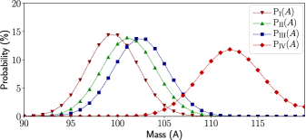
Figure 2: Mass fragmentation probabilities (light fragment) for all the configurations listed in Table 2.

The mass fragmentation probabilities are shown in Figure 2. We note that all curves are smooth and are peaked near the values of $A$ corresponding to the geometric split between the fragments. There is no visible odd-even staggering (OES) for any of the mass probabilities. In the case of the charge fragmentation probabilities shown in Figure 3, we note that the maximum of each curve is always associated with an even number of protons. Moreover, the probability for any even-proton number is always higher than the probability of any of the two odd-proton neighbors. In other words, we observe a clear OES. The different behavior of the mass and charge fragmentations is most likely caused by the Coulomb potential between the fragments, which increases the height of the effective barrier between them and, therefore, tends to localize the protons better than the neutrons.

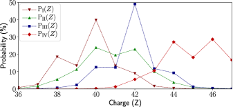
Figure 3: Charge fragmentation probabilities (light fragment) for all the configurations listed in Table 2.

Note that the fragmentation probabilities shown in Figure 2 and Figure 3 cannot be compared to experimental data Schillebeeckx et al. (1992); Nishio et al. (1995): They give only the dispersion around four specific fragmentations. In contrast, experimental fission fragment distributions include all possible fragmentations of the compound nucleus. To compare with experimental data, the first step is to explicitly simulate the nuclear dynamics, e.g., with semiclassical methods, such as Langevin or random walk Nadtochy and Adeev (2005); Nadtochy et al. (2007); Sadhukhan and Pal (2011); Nadtochy et al. (2012); Aritomo et al. (2015); Sadhukhan et al. (2016); Usang et al. (2016); Ishizuka et al. (2017); Sierk (2017); Usang et al. (2017); Randrup et al. (2011); Randrup and Möller (2011, 2013); Möller and Ichikawa (2015); Ward et al. (2017) or microscopic methods, such as the time-dependent generator coordinate method Goutte et al. (2004, 2005); Regnier et al. (2016); Zdeb et al. (2017); Tao et al. (2017); Zhao et al. (2019); Regnier et al. (2019). This would provide the probability distribution $\mathbb{P}({\mathcal{S}})$ for the nucleus to be in a given scissionned or quasiscissionned state $\mathcal{S}$. The second step would be to fold the probability distribution thus obtained with the probabilities $\mathbb{P}_{\mathcal{S}}({A})$ or $\mathbb{P}_{\mathcal{S}}({Z})$ that our method provides via

$$Y(X) =\sum_{\mathcal{S}}\mathbb{P}({\mathcal{S}})\mathbb{P}_{\mathcal{S}}({X}),\quad X=Z,A$$ (31)

$$Y(A,Z) =\sum_{\mathcal{S}}\mathbb{P}({\mathcal{S}})\mathbb{P}_{\mathcal{S}}({A})\mathbb{P}_{\mathcal{S}}({Z}).$$ (32)

Note that even if we do not consider correlations between protons and neutrons in the fragment probabilities in our method, the yields $Y(A,Z)$ obtained with the dynamics contains them.

III.3 Numerical Convergence

The MC method of Sec. II.2 is statistical and relies on sampling a probability distribution. When pairing correlations are included, the sampling is characterized by two numbers: $n_{\rm pair}$, the number of draws of the particle Slater determinants (first step of the algorithm presented in Sec. II.2.3, p. II.2.3), and $n_{\rm loc}$, the number of draws of a localized Slater determinant of $A$ particles from the left or right basis [cf. Eq. (8)]. Here, we evaluate the uncertainty associated with these two integers for the particular case of configuration II in Table 2.

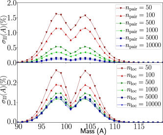
Figure 4: Standard deviations associated with the probabilities to measure the light fragment with a mass $A$ for the shape II. Top: For different values of $n_{\rm pair}$ and with $n_{\rm loc}=10\,000$. Bottom: For different values of $n_{\rm loc}$ and with $n_{\rm pair}=10\,000$.

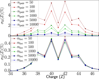
Figure 5: Same as Figure 4 for the charge fragmentations.

We considered 12 cases: $n_{\rm pair}=50$, $100$, $500$, $1\,000$, $5\,000$, $10\,000$ with $n_{\rm loc}=10\,000$; and $n_{\rm pair}=10000$ with $n_{\rm loc}=50$, $100$, $500$, $1\,000$, $5\,000$, $10\,000$. For each of them, we calculated the fragmentation probability in mass and charge $S=200$ times. We then calculated the unbiased estimator of the standard deviation $\sigma_{\mathrm{II}}(X)$ for the distributions in mass and in charge using the following expression, for $X=A,Z$:

$$\sigma_{\mathrm{II}}(X)\equiv\sqrt{\frac{1}{S-1}\sum_{k=0}^{S-1}\big{[}Y^{(k)}_{\mathrm{II}}(X)-\bar{Y}_{\mathrm{II}}(X)\big{]}^{2}},$$ (33)

where $Y^{(k)}_{\mathrm{II}}(X)$ is the $k$th calculation of the yields with our method and $\bar{Y}_{\mathrm{II}}(X)$ is the mean value of all the $Y^{(k)}_{\mathrm{II}}(X)$. The standard deviations are shown in Figure 4 for the mass distributions, and in Figure 5 for the charge distributions. The most sensitive parameter is $n_{\rm pair}$ with an improvement of 1.6% of the standard deviations on the masses and 5.5% on the charges between the cases $n_{\rm pair}=50,n_{\rm loc}=10\,000$ and $n_{\rm pair}=n_{\rm loc}=10\,000$ as shown in the upper panels of Figure 4 and Figure 5. For all the cases with $n_{\rm pair}=10\,000$, the standard deviations are always below 0.5%, and the improvement of the standard deviations is below 0.2% for the masses and not visible for the charges between the cases $n_{\rm loc}=50$ and $n_{\rm loc}=10\,000$.

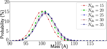
Figure 6: Probabilities to measure the light fragment with a mass $A$ for the shape II for different number of shells $N_{\mathrm{sh}}$ in the basis.

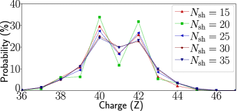
Figure 7: Same as Figure 6 for the charge of the light fragment.

The two other numerical parameters in our method are the number of shells $N_{\mathrm{sh}}$ and the truncation in the BCS occupation numbers $v^{2}_{\mathrm{thresh}}$. To analyze the impact of $N_{\mathrm{sh}}$, we have calculated the fragmentation probabilities in mass and charge for $N_{\mathrm{sh}}=15,20,25,30,$ and $35$ in the case of the configuration II. The corresponding curves are presented in Figure 6 and Figure 7. The increase in the number of shells shifts the most probable mass of the light fragment from $A=100$ to $A=101$ (and, therefore, shifts the most probable mass of the heavy fragment from $A=140$ to $A=139$). The increase of the number of shells does not change the most probable charge of the fragments. However, it drastically reduces the OES in the charge distribution between the cases $N_{\mathrm{sh}}=15$ and $N_{\mathrm{sh}}=35$.

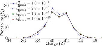
Figure 8: Probabilities to measure the light fragment with a charge $Z$ for the shape II different values $v^{2}_{\mathrm{thresh}}$ of the occupation numbers’ threshold.

To study the influence of the BCS occupations $v^{2}_{\mathrm{thresh}}$, we have calculated the fragmentation probability in mass and charge for the four cases $v^{2}_{\mathrm{thresh}}=1.0\times 10^{-1},2.8\times 10^{-3},1.7\times 10^{-9},1.0\times 10^{-15}$. The corresponding probabilities are shown in Figure 8 for the charge distributions only. All the distributions for the mass and the charges have converged below 1% for $v^{2}_{\mathrm{thresh}}\leq 2.8\times 10^{-3}$.

IV Number of Particles at Scission

In this section, we apply both the MC sampling and the projector methods to estimate the dispersion in particle number of realistic scission configurations for the case of ²⁴⁰Pu.

IV.1 Macroscopic-microscopic Calculations

First, we compare our approach with the projector method presented in Refs. Simenel (2010); Scamps and Lacroix (2013) for the macroscopic-microscopic approach. The Schödinger equation was solved in a basis of $N_{\rm sh}=35$ shells. Pairing correlations are treated in the same way as in Sec. III.3. We consider a scission configuration in ²⁴⁰Pu characterized by the following values of the 3QS parameters: $r_{\rm neck}=2.50$ fm, $\alpha_{2}=0.448$, $\alpha_{3}=0.6259$, $\sigma_{1}=3.0613$, $\sigma_{2}=-0.5349$, and $\sigma_{3}=0.9047$. This configuration corresponds to the most likely trajectory for a series of random walks on the five-dimensional potential energy surface Verrière et al. (2019).

Starting from this initial configuration, we vary the parameter $\sigma_{2}$ in order to reduce the size of the neck, and thus, approach the limit of two orthonormal s.p. bases for each of the prefragments. In practice, the values of $\sigma_{2}$ were chosen such that the neck radius takes the values $0.04$, $1.0$, $1.25$, $1.5$, $1.75$, $2.0$ fm. Figure 9 gives a visual representation of these configurations. For the MC sampling, we use $n_{\rm pair}=10\,000$ and $n_{\rm loc}=1\,000$; together with our basis size of a $N_{\rm sh}=30$ and a BCS threshold of $v^{2}_{\rm thresh}=10^{-5}$, this gives a statistical precision of approximately 0.5% on the charge and 0.15% on the mass fragmentation probabilities.

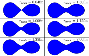
Figure 9: Geometric shapes associated with the scission configurations of Table 3.

Table 3: Characteristics of scission configurations: neck radius, shape parameters and average mass/charge fragmentations of the left fragment.

$r_{\rm neck}$	$\alpha_{2}$	$\alpha_{3}$	$\sigma_{1}$	$\sigma_{2}$	$\sigma_{3}$	$A_{\rm L}$	$Z_{\rm L}$
0.04	0.448	0.6259	3.0613	-0.8431	0.9047	138.8	53.1
1.00	0.448	0.6259	3.0613	-0.7876	0.9047	139.5	53.5
1.25	0.448	0.6259	3.0613	-0.7576	0.9047	139.8	53.7
1.50	0.448	0.6259	3.0613	-0.7219	0.9047	140.1	53.8
1.75	0.448	0.6259	3.0613	-0.6812	0.9047	140.6	54.0
2.00	0.448	0.6259	3.0613	-0.6361	0.9047	141.4	54.3

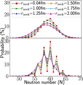
Figure 10: Upper panel: Neutron fragmentation probabilities (light fragment) for all the configurations listed in Table 3 obtained with our method. Lower panel: same probabilities obtained with the method presented in Simenel (2010).

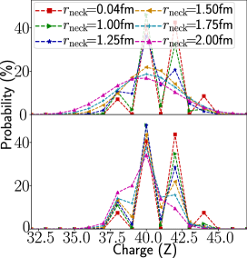
Figure 11: Same as Figure 10 for the charge fragmentation probabilities (color online).

The neutron fragmentation probabilities are shown in Figure 10: the top panel shows results with MC sampling, while the bottom panel shows results with projectors. We first note that there are substantial differences between the two approaches. Projectors yield an OES in the neutron fragmentations probabilities for $r_{\rm neck}<2.00$ fm. In contrast, there is no such OES in the sampling method except for very small values of the neck radius ($r_{\rm neck}<0.50$ fm).

The main explanation for this discrepancy is related to the parametrization of the nuclear surface. In generating the family of shapes of Figure 9, we started from the 3QS parameters corresponding to $r_{\rm neck}=2.5$ fm, and reduced only the value of $\sigma_{2}$ to obtain the other shapes. As a consequence of volume conservation, the fragments become more and more oblate with decreasing values of $r_{\rm neck}$, which increases the value of the neutron Fermi energy. This facilitates tunneling for the states with energies around and above the Fermi level, even more so since pairing correlations for neutrons are rather high with our parametrization of the pairing force (the pairing gap is of the order of $\Delta_{n}\approx 2.25$ MeV for all configurations). This spurious “geometrical” effect could have been avoided with a more rigorous exploration of the nuclear shapes around our initial scission configuration, by making sure that, as we vary the size of the neck, all deformation parameters are adjusted so that the the energy remains a minimum. Such an exploration of the deformation space is automatic in self-consistent calculations, but should be done by hand in semi-phemenological methods. The cost of doing so in a a five-dimensional PES as the one we were working with is rather substantial.

Because of the Coulomb barrier, the proton Fermi energy is much lower than the top of the barrier between the two prefragments: Tunneling is much less of an issue, and protons are better localized. This could explain why the agreement between the two methods is much better for the charge fragmentation probabilities, as shown in Figure 11: The probability associated with an odd $Z$ vanishes for a value of $r_{\rm neck}$ below 1.00 fm with both methods, and a strong OES appears, at $r_{\rm neck}=1.25$ fm for the MC sampling and at $r_{\rm neck}=1.75$ with projectors. The quantitative agreement between the two approaches is, in fact, relatively good for $r_{\rm neck}\leq 1$ fm.

IV.2 EDF Calculations

To gain further insight, we performed similar calculations in a fully microscopic framework. Specifically, we considered the scission configurations near the most likely fission of ²⁴⁰Pu which are discussed extensively in Sec. IV of Ref. Schunck et al. (2014). These configurations were obtained by performing constrained HFB calculations with $\langle\hat{Q}_{20}\rangle=345$ b and $\langle\hat{Q}_{\rm neck}\rangle$ varying between 0.1 and 4.5. All calculations were performed with the Skyrme SkM* energy functional; numerical details, such as the size and characteristics of the basis, the parameters of the pairing force, etc., can be found in Ref. Schunck et al. (2014).

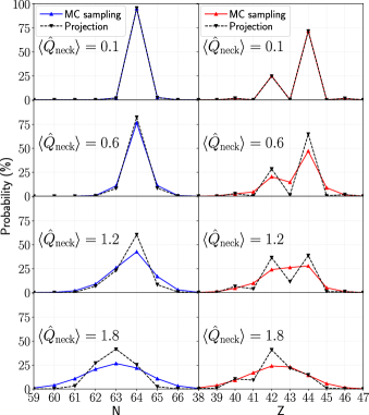
Figure 12: Left panel: Comparison of the neutron fragmentation probabilities obtained with our Monte Carlo sampling (full lines) and the projection method (dashed black lines) for different values of $\langle\hat{Q}_{\rm neck}\rangle$. Right panel: same for the proton fragmentations (color online).

For each value of the Gaussian neck parameter, we used the double-projection method to estimate the fragmentation probabilities of the system. We also computed the occupation probabilities $v_{k}^{2}$ in the canonical basis as well as the coefficients $\alpha_{k}$ of Eq. (8) needed for the MC method. Fig. 12 summarizes the results for the proton and neutron fragmentation probabilities obtained in the two methods.

We note that the agreement between projection and MC sampling at the limit of very small necks is much better than in the macroscopic-microscopic approach. One might attribute this better agreement to the fact that, in HFB calculations, the shapes of both the fissioning nucleus and the prefragments are automatically determined so that the energy of the fissioning system is minimum. As a consequence, such self-consistent calculations do not suffer from the geometrical artifact described in the previous section and the Fermi energy of both protons and neutrons does not vary much in the range of $\langle\hat{Q}_{\rm neck}\rangle$ considered here, in contrast to the macroscopic-microscopic case.

V Conclusion

We have presented a new method to estimate the uncertainty of particle number in the fission fragments. It relies on sampling the probability distribution of finding $N$ particles in the fragments based solely on the knowledge of a relevant s.p. basis for the fissioning nucleus together with occupation probabilities. We showed that our approach can be used to emulate results of particle-number projection techniques, but also provides s.p. bases for each subsystem – provided the latter are sufficiently well separated. We emphasize that it is applicable both for Slater determinants and for generalized Slater determinants (= quasiparticle vacuum of the HFB theory) and is readily applicable when the energy states are not degenerate (e.g., when parity is internally broken). Indeed, when parity is conserved, s.p. or quasiparticles are, by definition, spread over the two prefragments, and the splitting of the individual particle states might lead to nonorthogonal bases for each parition. In such cases, the degree of orthogonality of the basis within each partition should be tested to know if the Monte Carlo sampling method is applicable.

We showed that restoring the particle number in the prefragments formed at scission produces an odd-even staggering of probability fragmentations. When combined with full simulations of fission dynamics, this result could be key to reproducing the experimentally observed OES of the charge distributions. In addition, restoring the particle number could also be used to eliminate one of the free parameters typically associated with the calculations of fission fragment distributions (folding with a Gaussian, see Regnier et al. (2018)).

While we have illustrated our method in the case of the fission process of heavy atomic nuclei, it is, in principle, applicable to a much broader range of problems, such as, for example, the localization of electrons inside a molecule. In this case, space partitions would correspond to a small volume near each nucleus of the molecule, and we could calculate the number of electrons around each of them.