Region-Referenced Spectral Power Dynamics of EEG Signals: A Hierarchical Modeling Approach

Abstract

Functional brain imaging through electroencephalography (EEG) relies upon the analysis and interpretation of high-dimensional, spatially organized time series. We propose to represent time-localized frequency domain characterizations of EEG data as region-referenced functional data. This representation is coupled with a hierarchical regression modeling approach to multivariate functional observations. Within this familiar setting, we discuss how several prior models relate to structural assumptions about multivariate covariance operators. An overarching modeling framework, based on infinite factorial decompositions, is finally proposed to balance flexibility and efficiency in estimation. The motivating application stems from a study of implicit auditory learning, in which typically developing (TD) children, and children with autism spectrum disorder (ASD) were exposed to a continuous speech stream. Using the proposed model, we examine differential band power dynamics as brain function is interrogated throughout the duration of a computer-controlled experiment. Our work offers a novel look at previous findings in psychiatry, and provides further insights into the understanding of ASD. Our approach to inference is fully Bayesian and implemented in a highly optimized Rcpp package.

arXiv:0000.0000

T1This work was supported by the grant R01 MH122428-01 (DS, DT) from the National Institute of Mental Health.

, , , , , , and

1 Introduction

The human brain and its functional relation to biobehavioral processes like motor coordination, memory formation and perception, as well as pathological conditions like Parkinson’s disease, epilepsy, and autism have been a subject of intense scientific scrutiny Broyd et al. (2009), Uhlhaas and Singer (2010), Murias et al. (2007). An important and highly prevalent imaging paradigm aims to study macroscopic neural oscillations projected onto the scalp in the form of electrophysiological signals, and record them by means of electroencephalography (EEG).

Currently, a typical multi-channel EEG imaging study is carried out with a geodesic EEG-net, composed of up to 256 electrodes. After precise placement on the scalp, electrodes collect electrophysiological signals at high time-resolution, through event-related potentials (ERP) or event-related oscillations (ERO). In this setting, endogenous or exogenous events can result in frequency-specific changes to ongoing EEG oscillations. The spectral features of the resulting time-series are often used to quantify such changes. Specifically, in a time-frequency analysis, the spatiotemporal dynamics of frequency-specific power are examined as they relate to sensory, motor and/or cognitive processes Scheffler et al. (2018) Gou, Choudhury and Benasich (2011) Mills, Coffey-Corina and Neville (1993).

Our work is motivated by a study of language acquisition in young children with autism spectrum disorder (ASD), a developmental condition that affects an individual’s communication and social interactions Lord et al. (2000). It is thought that typically developing (TD) infants, as young as 6 months old, start to parse continuous streams of speech to actively discern word patterns Kuhl (2004). Infants diagnosed with ASD, tend to feature late development of linguistic skills Eigsti et al. (2011). Because, neither verbal instructions nor behavioral evaluations can be performed on toddlers, EEG platforms have been recognized as an effective and non-invasive functional brain imaging tool.

In an idealized setting, for each study unit we aim to characterize variability in the relative log-power of a specific frequency band, recorded at a scalp location $s$, at time $t$. This aim is, however, complexed by several estimation- and data-related challenges. Raw EEG recordings, in fact, suffer from exogenous contamination, poor spatial resolution, as well as non-stationarity. To mitigate these issues, several pre-processing and regularization strategies have been proposed in the literature Scheffler et al. (2018). In this article, we build on our previous work and couple the characterization of EEG spectral dynamics as region-referenced functional data with a Bayesian model for multivariate functional observations. Fig. 1 illustrates the fundamental nature of the data structures considered in our motivating case study, by depicting specific band power trajectories through time-in-trial and across 3 of 11 brain regions in a study of language acquisition. Given this data structure, we are interested in region-specific, time-varying differences in band power dynamics between diagnostic groups. Crucially, valid inference depends on the correct specification of large multivariate covariance functions.

Many approaches to functional data analysis rely on functional principal components analysis as a fundamental tool for advanced modeling Yao, Müller and Wang (2005) James, Hastie and Sugar (2000). Methods for the analysis of multivariate functional data are more sporadic, but tend to follow similar strategies with specific attention paid to data scales Chiou, Chen and Yang (2014) or potential heterogeneity in the functional evaluation domain Happ and Greven (2018). The Bayesian literature on the subject is more sparse, with notable exceptions to be found in Baladandayuthapani et al. (2008), who consider nested spatially correlated functional data under assumptions of separability, and the more general work of Zhou et al. (2010), who consider similar data structures under more flexible covariance models.

The use of typical spatial assumptions is, however, problematic in the analysis of region-referenced EEG data. Namely, Euclidean distances between electrodes may not accurately characterize functional dependency of within-subject relative log-power readings. Therefore, instead of relying on pre-specified covariance structures (e.g. conditionally autoregressive models) to describe within-subject correlation, we propose to estimate them through functional factor analysis.

In particular, this article introduces a probabilistic framework for multivariate functional data regression which hinges on two ideas, (1) the constructive definition of Gaussian Processes through basis expansions, and (2) the modeling of covariance operators through functional factor analysis Montagna et al. (2012a). While neither approach is new, we highlight the application of these concepts to functional brain imaging though EEG. In the process, we discuss important consequences associated with specific implementation choices as they relate to transparent assumptions on the structure of multivariate covariance functions. Our proposal seeks to develop a general framework for automatic shrinkage and regularization through infinite factor models Bhattacharya and Dunson (2011). The resulting methodology is suitable for nonparametric estimation with any projection methods, which is amenable for use in a broad range of applications.

The article is organized as follows. In Section 2, we outline a conceptual framework for region-referenced band powers dynamics. A hierarchical functional model for region-referenced functional data is introduced in Section 3. We assess the performance of the proposed model on engineered datasets in Section 4, and apply our work to a neurocognitive study on auditory implicit learning in Section 5. We conclude with a critical discussion of our work in Section 6.

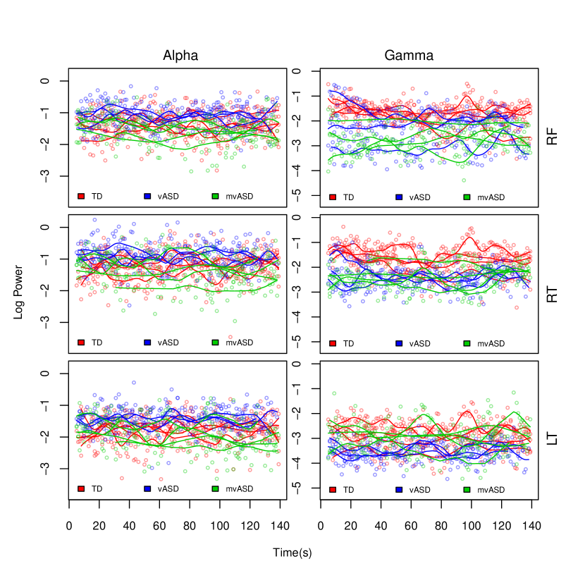
Figure 1: Power Dynamics in Language Acquisition. Log power dynamics both raw and smoothed, in three of eleven anatomical regions: (LT) left temporal, (RT) right temporal, and (RF) right frontal. For each region, we plot the principal component power for two frequency bands (Alpha, Gamma) during time on trial. We select three subjects from each of the three diagnostic groups: (TD) typically developing, (vASD) verbal ASD, and (mvASD) minimally verbal ASD.

2 Time-dependent Region-referenced Band-Power

EEG signals, measured through high resolution geodesic networks of electrodes, allow for highly localized interrogation of cortical functions throughout the duration of a computer-controlled experiment. In large studies, the high-dimensional nature of the resulting time series poses potential modeling and computational challenges.

Due to spatial proximity, neighboring electrodes collect signals likely to be highly multicollinear. In this context, the analysis of EEG data is often preceded by a dimension reduction exercise, aimed at discarding redundant information and aid interpretation through the definition of region-level summaries. Specifically, electrodes are partitioned according to anatomical regions on the scalp. Subsequently, region-level summaries are defined by averaging power spectra or by selecting the power spectrum of a single electrode within the region. Alternatively, given that multicollinearity of signals defines similarity in their spectral features, spectral PCA Brillinger (1981) has been proposed to pool information within anatomical regions with minimal loss of information. Applications to EEG data have been recently proposed by Ombao and Ho (2006), and Scheffler et al. (2018). Our approach follows closely the development in Scheffler et al. (2018), who perform spectral PCA on non-overlapping EEG segments. Our target summaries however focus on specific frequency bands as opposed to the entire power spectrum.

We outline and define basic concepts used in our work and defer details to Section 2 of the Supplement Li et al. (2020a). Let $\bm{X}_{ij}(s,t)$ denote the raw EEG recording, conceptualized as a locally stationary, zero-mean $q_{j}$-dimensional random process observed on subject $i$, $i=1,\ldots,n$, within anatomical region $j$, $j=1,\ldots,p$, for segment $t$, $t=1,\ldots,m$, at a sampling rate $U$ across discretized time $s$, $(s=0,\pm 1,\ldots,\pm U/2)$, assuming a 1s analysis window. For each observation $\bm{X}_{ij}(s,t)$, FFT is performed to obtain Fourier coefficients $\bm{d}_{ij}(\omega,t)=U^{-1/2}\sum_{s}\bm{X}_{ij}(s,t)\exp\{-i2\pi\omega s\}$, at frequency $\omega$. The raw periodogram matrix $\bm{I}_{ij}(\omega,t)=\bm{d}_{ij}(\omega,t)\overline{\bm{d}_{ij}}(\omega,t)^{\prime}$ is computed, where $\overline{\bm{d}_{ij}}(\omega,t)^{\prime}$ is the transpose of the complex conjugate of $\bm{d}_{ij}(\omega,t)$. Following Ombao and Ho (2006), we define kernel smoothed spectral density matrices $\tilde{\bm{I}}_{ij}(\omega,t)$, by smoothing $\bm{I}_{ij}(\omega,t)$ across $\omega$, using a Daniell kernel with bandwidths selected through generalized cross validation (GCV). Crucially, smoothing bandwidth are held fixed within region, resulting in $\tilde{\bm{I}}_{ij}(\omega,t)$ being Hermitian and non-negative definite.

A one-dimensional region-level summary may be obtained by defining the principal power $\lambda^{*}_{ij}(\omega,t):=c_{ij}^{-1}(t)\,\max_{|\bm{z}|=1}\bm{z}^{\prime}\tilde{\bm{I}}_{ij}(\omega,t)\,\bm{z}$, as the normalized leading eigenvalue of $\tilde{\bm{I}}_{ij}(\omega,t)$, with $c_{ij}(t)=\int\lambda_{ij}^{*}(\omega,t)\,d\omega$. Within region, the principal power summarizes common frequency-level variation across electrodes along the direction of the leading eigenvector. In contrast to Scheffler et al. (2018), who consider region-referenced longitudinal-functional representations, we adopt a simplified view and focus on specific frequency bands. Specifically, for a frequency range $(\omega_{a},\,\omega_{b})$, this article emphasizes modeling the time-varying principal band power $\gamma_{ij}(t):=\int_{\omega_{a}}^{\omega_{b}}\lambda^{*}_{ij}(\omega,t)\,d\omega$.

In adults, typical frequency bands and their spectral boundaries are delta ($<$4 Hz), theta (4-8 Hz), alpha (8-15 Hz), beta (15-32 Hz), and gamma (32-50 Hz). This view is motivated by traditional approaches in neurocognitive science, which differentiate functionally distinct frequency bands as they are thought to target distinct neurocognitive and biobehavioral processes Saby and Marshall (2012).

3 Hierarchical Models for Region-referenced Functional Data

3.1 Data Projections

Given a frequency band of interest, let $Y_{ij}(t)=\log\{\gamma_{ij}(t)\}$ be the logarithm of the principal band power for subject $i$, anatomical region $j$, evaluated at time $t$. In practice, for each subject, only a finite number of observations are collected discretely at $\bm{t}_{i}=\{t_{i1},t_{i2},\ldots,t_{im_{i}}\}$. However, for ease of notation, and without loss of generality, we assume $t\in\mathcal{T}=[a,b]$. Collecting all region-level log band-power measurements into a $p$-dimensional vector $\bm{Y}_{i}(t)=\{Y_{i1}(t),\ldots,Y_{ip}(t)\}^{\prime}$, we characterize subject-level observations as possibly contaminated multivariate functional data. Specifically, let $\bm{f}_{i}(t)=\{f_{i1}(t),\ldots,f_{ip}(t)\}^{\prime}$ be a set of $p$-dimensional random functions, with each $f_{ij}(t)$, $j=1,\ldots,p$, in $\mathcal{L}_{2}(\mathcal{T})$, a Hilbert space of square integrable functions with respect to the Lebesque measure on $\mathcal{T}$. We assume,

$$\bm{Y}_{i}(t)=\bm{f}_{i}(t)+\bm{\epsilon}_{i}(t),\quad\bm{\epsilon}_{i}(t)\sim N_{p}(0,\bm{\Sigma_{\epsilon}}),$$ (3.1)

with residual covariance $\bm{\Sigma}_{\epsilon}=\text{diag}(\sigma_{\epsilon 1}^{2},\ldots,\sigma_{\epsilon p}^{2})$. Given $\bm{f}_{i}(t)$, at time $t$, $\bm{Y}_{i}(t)$ is assumed to arise from independent realizations of a heteroscedastic multivariate Gaussian distribution.

We characterize the random functions $\bm{f}_{i}(t)$ through finite-dimensional projections onto $q$ cubic $B$-spline bases $\bm{b}(t)=\{b_{1}(t),\ldots,b_{q}(t)\}^{\prime}$. Specifically, let $\bm{\Theta}_{i}=\{\theta_{ijk}\}\in\mathbb{R}^{p\times q}$ be a matrix of random basis coefficients, we express 3.1 as follows:

$$\bm{Y}_{i}(t)=\bm{\Theta}_{i}\bm{b}(t)^{\prime}+\bm{\epsilon}_{i}(t).$$ (3.2)

The representation above is readily available for hierarchical modeling. Given priors on $\bm{\Theta}_{i}$ and $\bm{\Sigma}_{\epsilon}$, standard posterior inference and computation applies to the seemingly challenging problem of modeling multivariate functional data. Crucially, if the elements of $\bm{\Theta}_{i}$ are assumed Gaussian, given $\bm{b}(t)$, the simple construction in 3.2 implies that $\bm{f}_{i}(t)$ follows a $p$-dimensional Gaussian process, with second-order properties fully determined by covariance assumptions on the random basis coefficients.

In the following sections we develop an overarching structure for prior specification, including possible dependence on covariate information, and discuss modeling strategies and their implications for flexibility and efficiency in estimation.

3.2 Hierarchical Priors and Dependence on Covariates

A typical study of functional brain imaging aims to relate subject-level time-stable covariate information $\bm{w}_{i}=(w_{i1},\ldots,w_{id})^{\prime}$, with a region-referenced dynamic outcome $\bm{Y}_{i}(t)$. We focus on the conditional expectation $E\{\bm{Y}_{i}(t)\mid\bm{w}_{i}\}=E(\bm{\Theta}_{i}\mid\bm{w}_{i})\,\bm{b}(t)^{\prime}$ as the principal measure of association between covariates and brain function outcomes. Let $M(\bm{w}_{i})\coloneqq E(\bm{\Theta}_{i}\mid\bm{w}_{i})$; a familiar modeling framework for $\bm{\Theta}_{i}$ relies on the following matrix mixed effects construction,

$$\bm{\Theta}_{i}=M(\bm{w}_{i})+\bm{Z}_{i},\quad\text{vec}(\bm{Z}_{i})\sim N_{pq}(0,\bm{\Sigma}_{z});$$ (3.3)

where $\bm{Z}_{i}\in\mathbb{R}^{p\times q}$ captures subject specific regional and functional variation. Assuming $\bm{w}_{i}$ is organized as a regression design vector, let $\bm{\Psi}_{\ell}\in\mathbb{R}^{p\times q}$, $\ell=1,\ldots,d$, be regression coefficients; a matrix linear model defines $M(\bm{w}_{i})=\sum_{\ell=1}^{d}\bm{\Psi}_{\ell}\,w_{i\ell}$. In this setting, the regression functions $\bm{\mu}_{\ell}(t)\coloneqq\bm{\Psi}_{\ell}\bm{b}(t)^{\prime}$, are $p$-dimensional varying coefficients, to be interpreted in relation to the design structure encoded in $\bm{w}_{i}$ Zhu, Li and Kong (2012).

Given a basis projection, the second order behavior indexing functional and region-level dependence for the the multivariate Gaussian process $\bm{f}_{i}(t)$ is fully determined by the covariance matrix $\bm{\Sigma}_{z}$. While finite-dimensional, this matrix is likely high-dimensional as its spans both the number of regions $p$, and a potentially large number of basis functions $q$. We discuss three modeling approaches, aimed at regularization through shrinkage and simplifying structural assumptions, namely: (NB) a Naïve-Bayes prior, (SS) a Separable Sandwich prior, and (NS) a regularized Non-Separable prior.

(NB) Naïve-Bayes Prior. This construction exploits two simplifying assumptions: (1) the random coefficients matrix $\bm{Z}_{i}$ is assumed to follow a Matrix Gaussian distribution, and (2) covariance along time is parametrized through Bayesian P-splines smoothing penalties Lang and Brezger (2004). Let $\bm{\Omega}_{0}\in\mathbb{R}^{q\times q}$ be a deterministic penalty matrix, and $\bm{S}\in\mathbb{R}^{p\times p}$ be a covariance matrix indexing dependence between anatomical regions. The NB prior assumes

$$\bm{Z}_{i}\sim\mathcal{M}\mathcal{N}(0,\bm{S},\bm{\Omega}_{0}^{-1}),\quad\quad\bm{S}^{-1}\sim W(\nu,\bm{S}^{-1}_{0}/\nu).$$ (3.4)

The prior above structures $\bm{\Sigma}_{z}=\bm{S}\otimes\bm{\Omega}_{0}^{-1}$, implying separability of covariation between regions and time points. The matrix $\bm{S}$ serves both the purpose of modeling dependence between brain regions through its off diagonal elements, and the purpose of establishing region-level adaptive smoothing through its diagonal elements as they multiply $\bm{\Omega_{0}^{-1}}$. More details about this matrix and the choice of hyperparameters are discussed in Web Appendix C. While greatly simplified, when compared to a completely unstructured $\bm{\Sigma_{z}}$, this construction is potentially problematic as it hinges on a relatively rigid parametrization for the time-covariance, while enforcing only mild Wishart regularization of $\bm{S}$.

(SS) Separable Sandwich Prior. A more balanced approach to the prior in 3.4 retains the assumption of separability, but implements adaptive regularized estimation of both the time and region covariance. In particular, we extend the approach of Montagna et al. (2012b), and propose a two-way Bayesian latent factor model for $\bm{Z}_{i}$. Let $\bm{\Upsilon}=\{\upsilon_{jr}\}\in\mathbb{R}^{p\times k_{1}}$, and $\bm{\Gamma}=\{\gamma_{vs}\}\in\mathbb{R}^{q\times k_{2}}$ be two loading matrices. Also let $\bm{H}_{i}=\{h_{rs}\}\in\mathbb{R}^{k_{1}\times k_{2}}$, be a random matrix with $h_{rs}\sim_{iid}N(0,1)$, $r=1,\ldots,k_{1}$, $s=1,\ldots,k_{2}$, we write:

$$\bm{Z}_{i}=\bm{\Upsilon}\bm{H}_{i}\bm{\Gamma}^{\prime}+\bm{R}_{i},\quad\quad\text{with}\quad\bm{R}_{i}\sim\mathcal{M}\mathcal{N}(\bm{0},\bm{\Sigma}_{p},\bm{\Sigma}_{q});$$ (3.5)

where $\bm{\Sigma}_{p}$ and $\bm{\Sigma}_{q}$, both are diagonal with anisotropic components. This construction, implies

$$\bm{\Sigma_{z}}=\bm{\Upsilon}\bm{\Upsilon}^{\prime}\otimes\bm{\Gamma}\bm{\Gamma}^{\prime}+\bm{\Sigma}_{p}\otimes\bm{\Sigma}_{q}.$$

Typically, as in latent factor models, a truncation $k_{1}<p$ and $k_{2}<q$ is selected to define a low-rank representation of the region and time covariances. Rather than selecting the number of latent factors, we consider the multiplicative shrinkage prior of Bhattacharya and Dunson (2011), so that:

$$\upsilon_{jr}\mid\phi_{jr},\tau_{r}\sim\text{N}(0,\phi_{jr}^{-1}\tau_{r}^{-1}), \quad\phi_{jr}\sim\text{Ga}(\nu_{1}/2,\nu_{1}/2),\quad\tau_{r}=\prod_{u=1}^{r}\delta_{u},$$

$$\delta_{1}\sim\text{Ga}(a_{11},1), \quad\delta_{u}\sim\text{Ga}(a_{12},1),\quad\text{when }u>1;$$

$$\gamma_{vs}\mid\rho_{vs},\kappa_{s}\sim\text{N}(0,\rho_{vs}^{-1},\kappa_{s}^{-1}), \quad\rho_{vs}\sim\text{Ga}(\nu_{2}/2,\nu_{2}/2),\quad\kappa_{s}=\prod_{\ell=1}^{s}\pi_{v},$$

$$\pi_{1}\sim\text{Ga}(a_{21},1), \quad\pi_{v}\sim\text{Ga}(a_{22},1),\quad\text{when }\ell>1.$$

When $a_{11}>1,a_{12}>1$, this prior defines stochastically increasing precisions as more columns are added to $\bm{\Upsilon}$ and $\bm{\Gamma}$. Specific details about this shrinkage strategy and choice of hyperparameters are reported in the Supplement (Section 3) Li et al. (2020a). In what follows, we build on latent factor representations and forego the assumption of separability altogether.

(NS) Non-Separable Prior. As noted in Cressie and Huang (1999), the class of separable models (3.4, 3.5) is severely limited since it cannot capture region-time interaction. The cross-covariance functions between the time series at any region has the same shape, regardless of region location. Separable structures are often chosen for convenience rather than for their ability to fit the data well. These limitations make the separability approach difficult to justify in the setting of functional neuroimaging. A simple approach, which foregoes this assumption, while still defining a regularized representation of $\bm{\Sigma}_{z}$ involves dealing with $\mbox{vec}(\bm{Z}_{i})$ directly. Specifically, let $\bm{\Xi}=\{\xi_{cs}\}\in\mathbb{R}^{pq\times k}$, be a loading matrix, and $\bm{\eta}_{i}\sim N_{k}(0,I_{k})$, we write

$$\text{vec}(\bm{Z}_{i})=\bm{\Xi}\,\bm{\eta}_{i}+\bm{r}_{i},\quad\quad\text{with}\quad\bm{r}_{i}\sim N_{pq}(0,\bm{\Sigma}_{r}),$$ (3.6)

with $\bm{\Sigma}_{r}=\mbox{diag}(\sigma^{2}_{r1},\ldots,\sigma^{2}_{rpq})$, implying $\bm{\Sigma}_{z}=\bm{\Xi}\,\bm{\Xi}^{\prime}+\bm{\Sigma}_{r}$. This formulation leads to a probabilistic version of the multivariate FPCA of Chiou, Chen and Yang (2014), with normalization handled through explicit assumptions of heteroscedasticity through $\bm{\Sigma}_{r}$. Echoing the approach used in the sandwich prior, the model is completed with a shrinkage prior on the loading matrix $\bm{\Xi}$, so that

$$\bm{\xi}_{(s)}^{(c)}\mid\bm{\Omega}_{s},\tau_{c}\sim N\left({\bm{0},\,\bm{\Omega}_{s}^{-1}\tau_{c}^{-1}}\right), \quad\bm{\Omega}_{s}\sim\text{W}(\nu,\bm{\Omega}_{0}/\nu),\quad\tau_{c}=\prod_{l=1}^{c}\delta_{l},$$

$$\delta_{1}\sim\text{Ga}(a_{1},1), \quad\delta_{l}\sim\text{Ga}(a_{2},1),\quad\text{when }l>1;$$

where $\bm{\xi}_{(s)}^{(c)}$ indicates the $s$-th $p$-dimensional block, $s\in\{1,\ldots,q\}$, of the $c$-th column of $\bm{\Xi}$, $c=1,\ldots,k$.

It is easy to show that the vectorized model in 3.6 encompasses both the separable sandwich prior in 3.5 and the naïve-Bayes prior in 3.4. We examine the finite sample properties of these modeling strategies under several simulation scenarios in the section 4.

The three priors listed above span a broad range of model flexibility. We recognize, however, that several other nuanced configurations have been considered in the literature; particularly, when sampling schedules allow for design-driven structural assumptions. For example, in the context of longitudinal functional data, methodological simplifications to multivariate functional data, include both functional random effects models Greven et al. (2010) and simplified multivariate functional principal components representations Park and A (2015). Weakly separable covariance structures have been characterized in Chen and Lynch (2017), bridging the complexity of SS and NS models, by expressing a multi-way covariance as the linear combination of rank-one strongly-separable terms. This idea has found several applications and extensions in the context of longitudinal functional data literature Lynch and Chen (2018); Scheffler et al. (2020); Shamshoian et al. (2019). While a comprehensive comparison is out of scope for this work, in the context of our case study and through simulations, we aim to assess how a general NS model can avoid losses in efficiency through adaptive regularization.

3.3 Posterior Inference

Posterior inference is based on Markov Chain Monte Carlo simulations from the target measure. All prior models discussed in section 3.2 are amenable to simple Gibbs Sampling implementations. A highly optimized R package for data manipulation and inference is freely available from github at https://github.com/Qian-Li.

The MCMC transition schedule implemented in our package is optimized to marginalize out subject by region coefficients whenever possible, therefore limiting the degree of autocorrelation between posterior draws. As is the case with GP-type regression, in applying our method beyond EEG data, some care is needed, as the scalability of simple posterior sampling schemes could be an issue in high-dimensions (large $n$ or $p$). In these cases, specialized approximation strategies are, however, applicable as described in Nishimura and Suchard (2018).

We note that the loading matrix $\bm{\Xi}$ in 3.6, as well as $\bm{\Upsilon}$ and $\bm{\Gamma}$ in 3.5 are not likelihood-identified due to invariance to orthogonal rotations. Crucially, however: $\bm{\Xi}\bm{\Xi}^{\prime}$, $\bm{\Upsilon}\bm{\Upsilon}^{\prime}$ and $\bm{\Gamma}\bm{\Gamma}^{\prime}$ are all uniquely identified, leading to likelihood-identifiability of $\bm{\Sigma}_{z}$. Given posterior samples from the model parameters, Monte Carlo estimates of all quantities of interest, including simultaneous credible bands are obtained in a relatively straightforward fashion Baladandayuthapani, Mallick and Carrol (2005). Detailed calculations, including full conditional distributions are reported in the Supplement Li et al. (2020a).

4 Experiments on Engineered Data

To evaluate the finite sample performance of the hierarchical model and priors described in Section 3 we carried out an extensive Monte Carlo study considering data generated under several dependence structure (separable, non-separable), dependence strength, sample size, and signal-to-noise ratio scenarios. The signal-to-noise ratio is defined by $\text{SNR}=\frac{1}{n}\frac{1}{p}\sum_{i=1}^{n}\sum_{j=1}^{p}\int_{\mathcal{T}}f_{ij}(t)^{2}dt/\sigma_{\epsilon}^{2}$. Intuitively, SNR in this context can be intended as an inflation quotient for the error-variance $\sigma^{2}_{\epsilon}$. The general goal of these experiments aims to assess how well the mean $M(\bm{w}_{i})$ and covariance $\bm{\Sigma}_{z}$ are recovered under different priors and simulation truths. Further details regarding the data generation scheme are available in Web Appendix (Section 4).

Let $\hat{\bm{\mu}}_{\ell}(t)$ and $\widehat{\bm{\Sigma}}_{z}$ denote posterior mean estimates for their parametric counterparts (Section 3.2). To quantify the quality of estimates we consider relative squared errors, defined as follows:

• Mean: average relative squared error across regions and covariates, s.t.

  $$\text{RSE}(M)=\frac{1}{dp}\sum_{\ell=1}^{d}\left[\frac{\int_{t}\{\hat{\bm{\mu}}_{\ell}(t)-\bm{\mu}_{\ell}(t)\}^{2}\mathop{}\!\mathrm{d}t}{\int_{t}\bm{\mu}_{\ell}(t)^{2}\mathop{}\!\mathrm{d}t}\right]^{\prime}\bm{1}_{p};$$

• Covariance: Relative squared Frobenius error, st.

  $$\text{RSE}(\Sigma_{z})=\frac{\lVert\Sigma_{z}-\widehat{\Sigma}_{z}\rVert_{F}^{2}}{\lVert\Sigma_{z}\rVert_{F}^{2}}.$$

In relation to these metrics we observe the following behavior.

Table 1: Simulation Study. Mean and Covariance recovery under Naïve-Bayes (NB), Separable-Sandwich (SS), and Non-Separable (NS) priors. Relative errors are reported under separable and non-separable simulation truths, sample size escalation ($n=10,20,30$) and two signal-to-noise ratio scenarios ($SNR=0.2,1.0$).

	$n=10$		$n=20$		$n=50$
	Mean	Cov.	Mean	Cov.	Mean	Cov.
Separable	(SNR $=0.2$)
NB	0.0346	0.3255	0.0248	0.3150	0.0162	0.3120
SS	0.0384	0.3192	0.0272	0.3004	0.0174	0.2806
NS	0.0386	0.3380	0.0272	0.3117	0.0174	0.2900
	(SNR $=1.0$)
NB	0.0277	0.5146	0.0195	0.5126	0.0124	0.5180
SS	0.0272	0.1987	0.0192	0.1817	0.0122	0.1677
NS	0.0272	0.2595	0.0192	0.2294	0.0122	0.1915
Non-Separable	(SNR $=0.2$)
NB	0.0382	0.4217	0.0276	0.4189	0.0183	0.4226
SS	0.0413	0.3633	0.0289	0.3547	0.0185	0.3470
NS	0.0415	0.3427	0.0290	0.3188	0.0185	0.2892
	(SNR $=1.0$)
NB	0.0339	0.6601	0.0236	0.6110	0.0153	0.6164
SS	0.0340	0.3412	0.0235	0.3357	0.0152	0.3321
NS	0.0338	0.2721	0.0234	0.2433	0.0151	0.2101

Sample size and SNR. For each of 100 datasets, we simulate $n=10,20,50$ individuals in each of 3 diagnostic groups, with functional observations collected over 6 anatomical regions. Each data-set is considered under two signal-to-noise ratio scenarios, SNR$=0.2,1.0$. We assume observations are defined on a common time-grid $\in[0,1]$, with random missing patterns, where between $0$ and $80\%$ of the time-points are discarded to mimic observed data. Results are summarized in Table 1.

All three priors recover the mean structure equally well under both SNR scenarios. Independently of the generating dependence structure, average relative squared errors improve as more subjects are included for analysis. More meaningful differences are observed when we consider recovery of the covariance structure. When data are generated under separable covariance, SS priors exhibit the best performance, with improved accuracy for larger sample sizes. Some loss in efficiency is observed when considering NS priors. However, even with only 10 subjects the loss in efficiency is estimated to be only about 30%, reducing to about 4% when sample size escalates to $n=50$. When data are generated from non-separably covarying processes, NS priors exhibit the highest efficiency, and are the only model improving meaningfully in accuracy as sample size increases. In all simulation settings, NB priors seem to perform poorly in relation to other alternatives.

In summary, our findings agree with well known results in multivariate and longitudinal data analysis Wakefield (2013). Consistent recovery of the mean function seems to be relatively insensitive to the covariance model. Inference and uncertainty quantification about the mean, however, requires correct recovery of the dependence structure encoded in $\bm{\Sigma}_{z}$. While meaningful gains in efficiency can be achieved if separability assumptions are warranted in applications, the encompassing regularized prior (NS) leads to a generally more flexible and efficient modeling framework, without the need for stringent structural assumptions.

Extended results, including sensitivity to model specification are reported in the Supplement Li et al. (2020a). While theoretical large sample results are not examined in the manuscript, all simulation results can be reproduced and extended with our R package and supplementary documentation.

5 EEG and Language Acquisition in TD and ASD Infants

5.1 Study Background

We consider a functional brain imaging study carried out by our collaborators in the Jeste laboratory at UCLA. The study aims to characterize differential functional features associated with language acquisition in TD and ASD children. EEG data were recorded for 144s using an 128 electrode HydroCel Geodesic Sensor Net for 9 TD, 32 ASD children ranging between 4 and 12 years of age. The EEG data is divided into non-overlapping segments of 1.024 seconds, producing a maximum of 140 observable segments for each subject at each electrode. Details about data pre-processing are deferred to Web Appendix A. Individual sensors were partitioned between 11 anatomical regions made up of 4-7 electrodes; left and right for the temporal region (LT and RT) and left, right, and middle for the frontal, central, and posterior regions (LF, RF, MF, LC, RC, MC, LP, RP, and MP, respectively). Region-level power dynamics were estimated as outlined in Section 2. Figure 1 illustrates a sample of smoothed power trajectories within the alpha and gamma frequency bands for both TD and ASD children. ASD children were further classified as verbal ASD (vASD - 14 children) and minimally verbal ASD (mvASD - 19 children) in relation to their verbal Developmental Quotients (vDQ).

The broad scientific goal of this study aims to understand the functional underpinnings associated with language acquisition through the human ability to parse otherwise continuous speech streams into meaningful words. In order to replicate this natural phenomenon, children were exposed to continuous synthetic speech constructed through a collection of 12 phonemes. By defining phoneme triplets (e.g. pa-bi-ku, da-ro-pi) as deterministic pseudo-words and exposing children to random continuous permutations of pseudo-words, study subjects were given the opportunity for implicit statistical learning of word segmentation. During this process, we seek to detect differential neurophysiological response across anatomical regions and oscillation frequencies.

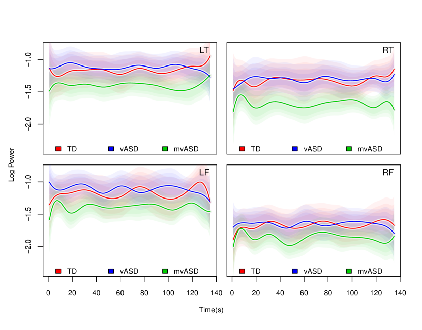
Figure 2: Alpha Power Dynamics. Average log power dynamics stratified by diagnostic group: (TD) typically developing, (vASD) verbal ASD, and (mvASD) minimally verbal ASD. Four of eleven anatomical regions are represented, namely: (LF) left frontal, (RF) right frontal, (LT) left temporal, and (RT) right temporal. In each region, we display the posterior mean, accompanied by simultaneous credible bands, shaded to include 0.2, 0.6, and 0.8 of all posterior samples.

5.2 Group Mean Trajectory Analysis

Our analysis focuses on time-varying region-referenced differences among diagnostic groups (TD, vASD, mvASD) in relation to two frequency bands, namely alpha (8-15 Hz), and gamma (32-50 Hz). Specifically, alpha waves are thought to play an active role in network coordination and communication Fink and Benedek (2014), while gamma waves are thought to index conscious perception and tend to correlate with implicit learning processes Gruber and Müller (2002).

Our analyses are based on the non-separable model in (3.6), with 10 latent factors, and data projected on 12 B-splines basis functions. Main findings across 4 of 11 regions are summarized graphically in Fig 2 for alpha waves and in Fig 3 for gamma waves. In both models, the varying coefficients representing the mean structure in 3.3, take as input a simple factorial covariate indexing diagnostic group membership, and yield group-level means across anatomical regions. For each time-varying mean, we also represent simultaneous credible bands by probability shading, to include a gradient of 0.2, 0.6 and 0.9 posterior coverage. A brief discussion about sensitivity to the prior model, number of latent factors, and projection methods is deferred to Section 6.

Starting with a group-by-region analysis of the alpha frequency band in Fig. 2, we note that for all three groups, across all 11 brain regions, there is no discernible time-varying pattern in the average relative alpha frequency, which is maintained relatively flat across time-in-trial. The TD and vASD groups are essentially indistinguishable, with minor differences likely due to sampling variability. Crucially, meaningfully lower levels in the average relative alpha frequency are observed for the mvASD group. While we fall short of considering formal notions of statistical significance, we highlight potentially meaningful findings in the RT region, where 90% simultaneous bands fail to overlap for some of the time-on-trial. More importantly, the lower level in relative alpha frequency is consistent across most brain regions, suggesting a potential role of alpha waves in distinguishing brain functional characteristics in the minimally verbal ASD group. Finally, within group, for all diagnostic groups, we confirm a well known phenomenon known as left-right alpha asymmetry, which is significant over time at frontal regions, diminished at temporal regions, and negligible at central and posterior regions.

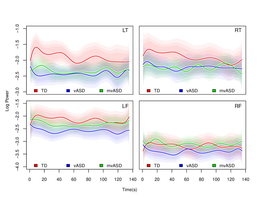
Figure 3: Gamma Power Dynamics. Average log power dynamics stratified by diagnostic group: (TD) typically developing, (vASD) verbal ASD, and (mvASD) minimally verbal ASD. Four of eleven anatomical regions are represented, namely: (LF) left frontal, (RF) right frontal, (LT) left temporal, and (RT) right temporal. In each region, we display the posterior mean, accompanied by simultaneous credible bands, shaded to include 0.2, 0.6, and 0.8 of all posterior samples.

Replicating the same analysis for gamma frequencies in Fig.2 we note that, while alpha waves seem to isolate the mvASD group, gamma waves tend to separate TD children from the vASD and mvASD groups. More precisely, the TD group exhibits significantly higher average gamma band power than vASD and mvASD, especially at the early stages of the experiment. This pattern is most evident at temporal regions, both left and right (LT, RT). Furthermore, the average gamma band power for TD children exhibits a sharp increase at the beginning of time-on-trial, followed by a decreasing trend through the end of the experiment. This finding suggests, that differently from the ASD groups, TD children consciously perceive the beginning of the speech stream as a stimulus. Compatible findings by Gruber and Müller (2002) report a decreased response when stimuli recur, which they projected to be linked to a “neural savings” mechanism within a cell assembly representing an object, i.e. a word in our case. As observed for alpha band power, we note significant frontal asymmetry throughout the study and across diagnostic groups. While previous studies, e.g. Rojas and Wilson (2014), pointed out left-dominant asymmetry as a discriminative feature between TD and ASD cohorts, our findings do not replicate this observation within the context of a language acquisition experiment.

We compared the NB, SS and NS prior models, by computing their expected log pointwise predictive density leave-one-out cross-validation (elpd-loo)Watanabe (2013); Vehtari, Gelman and Gabry (2017, 2015). In the context of our case study, let $p\{\bm{Y}_{i}(t)\mid\bm{Y}_{-i}(t)\}$ be the leave-one-out predictive density for subject $i$, ($i=1,\ldots,n$). The elpd-loo is computed as follows:

$$\text{elpd}_{\text{loo}}=\sum_{i=1}^{n}\log p(\bm{Y}_{i}(t)|\bm{Y}_{-i}(t))$$ (5.1)

Treating gamma band power as the response, NB has $\text{elpd}_{\text{loo}}=-11586$ (SE$=947$), SS with 6 latent factors for the time and spatial domains has $\text{elpd}_{\text{loo}}=-10981$ (SE$=911$), and NS with 10 latent factors has $\text{elpd}_{\text{loo}}=-10951$ (SE$=910$). Treating alpha power as the response, NB has $\text{elpd}_{\text{loo}}=-14698$ (SE$=1227$), SS has $\text{elpd}_{\text{loo}}=-14211$ (SE$=1209$), and NS has $\text{elpd}_{\text{loo}}=-14260$ ($SE=1214$). For both the gamma and alpha power bands, SS and NS tend have a relatively similar performance, while NB seems to underperform in both settings. Our analyses are therefore based on the NS prior, as it is more general and does not seem to induce any loss in predictive power for this case study.

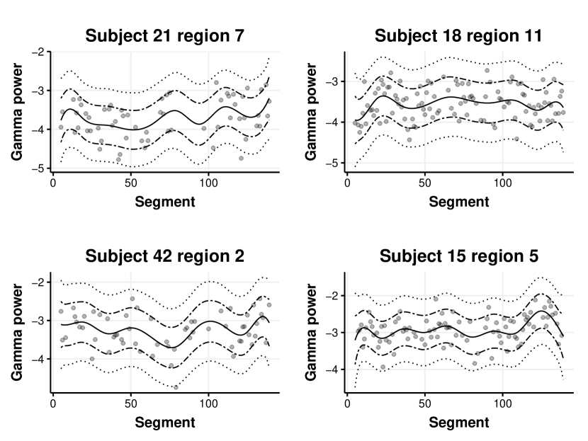
Figure 4: Gamma power goodness of fit. Posterior mean trajectory (solid line) for four random subject region responses. We report pointwise (dot-dash lines) and simultaneous (dotted lines) 90% posterior predictive credible bands. Top left: subject 21 (mvASD), region 7. Top right: subject 18 (ASD), region 11. Bottom left: subject 42 (mvASD), region 2. Bottom right: subject 15 (ASD), region 5.

To assess goodness of fit, we compute 90% pointwise and simultaneous (grouping by subject and region) posterior predictive credible bands treating gamma power as the response Gelman, Meng and Stern (1996). Simultaneous bands are obtained as in Crainiceanu et al. (2007). Figure 4 displays four random subject-region gamma power dynamics accompanied with maximum a posteriori fit and 90% pointwise posterior prediction bands . The figure illustrates adequate fit and predictive coverage for all four subjects. Over all subjects, the interquartile range (IQR) of predictive coverage rate is (78.4%, 88.5%) and (97.1% to 100%) using pointwise prediction bands and simultaneous prediction bands respectively. Similar IQR coverage rates are obtained when considering alpha power dynamics, indicating that the model is reasonably well calibrated Dawid (1985).

A frequentist test for goodness of fit was applied using the framework developed by Yuan and Johnson (2012). Although standardized residual means are consistently close to 0, the p-values for different quantile thresholding scenarios suggest some evidence of lack-of-fit with the residual variance model. A detailed analysis at two levels of the model hierarchy is reported in the supplement Li et al. (2020a). We note that, while these findings are unlikely to influence inference on population summaries, some care would be needed in predictive settings, where a scale mixture extension of the residual model would likely account for the observed overdispersion with respect to Gaussian sampling.

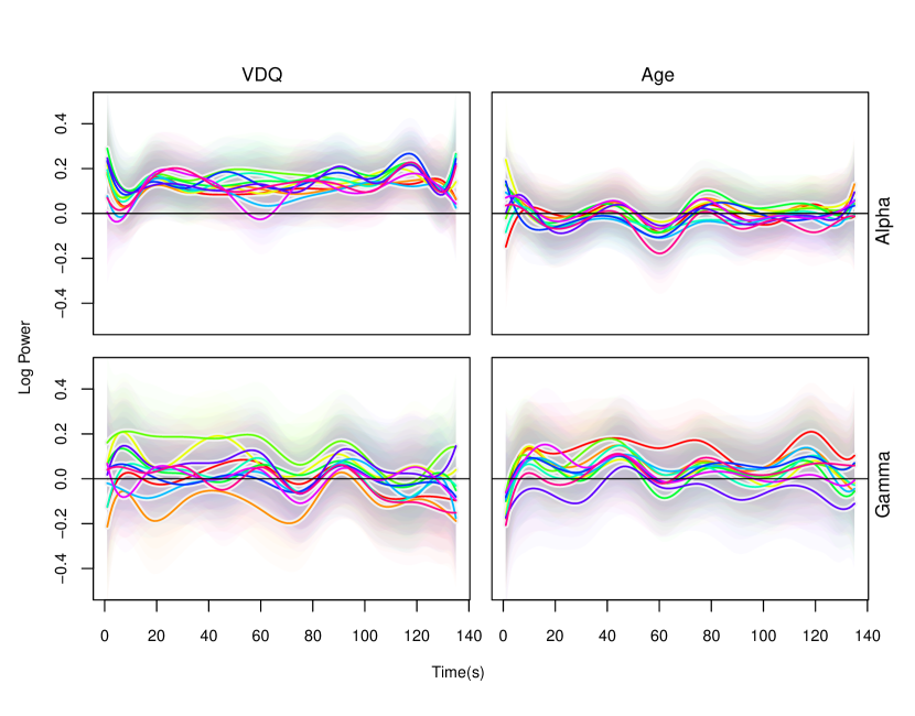
Figure 5: Varying Coefficients for Age and vDQ. Varying coefficients associated with age and verbal DQ across all anatomical regions for the Gamma and Alpha frequency bands. Each varying coefficient is accompanied by simultaneous credible bands, shaded to include 0.2, 0.6, and 0.9 of all posterior samples.

5.3 Effects of Age and Verbal-DQ

Rather than considering a coarse classification of subjects into TD, vASD and mvASD, we examine how alpha and gamma band power trajectories change as a function of age and verbal DQ. Due to the relatively small-sized sample, the distribution of subjects demographics among three groups is somewhat unbalanced. To be specific, the TD cohort is significantly older ($94.7\pm 28.8$, in months) with hider vDQ ($120.6\pm 11.4$), the v-ASD cohort are younger ($67.1\pm 58$) with medium vDQ ($89.3\pm 22.7$) and mv-ASD has a wide age-range ($85.6\pm 24.0$), however significantly lower by vDQ ($23.6\pm 10.9$). Our analysis is therefore not perfect, but still warranted under the assumption of generalized additive effects. In particular, the mean structure in 3.3 is represented as the additive combination of time-varying coefficients, including an intercept function, a coefficient function for the main effect of age and a coefficient function for the main effect of vDQ.

Our results are summarized graphically in Fig. 5. We display the varying coefficients for age and vDQ for both the alpha and gamma band power, across all 11 brain regions. For each curve we include probability shading for simultaneous 0.2, 0.6, and 0.9 credible bands. The effects of Age and vDQ on alpha band power is consistent across all brain regions. While age does not seem to be associated with the outcome, higher vDQ levels are consistently and significantly associated with higher alpha band power levels. This finding is consistent with the group-level analysis in Section 5.2, where mvASD children were found to exhibit significantly lower alpha levels, when compared to TD and vASD children. On the other hand, the relationship between vDQ and gamma band power is highly heterogeneous across brain regions, with vDQ positively associated with higher gamma band power in temporal regions (LT and RT) and negatively associated with the outcome in the right frontal regions (RF). The effect of Age on gamma power is more consisted across brain regions, with older children exhibiting higher gamma in some regions, and significantly so in LF.

6 Discussion

We introduced a hierarchical modeling framework for the analysis of region-referenced functional data in the context of functional brain imaging through EEG. Our work hinges on two classical ideas, namely: the constructive definition of Gaussian processes through basis functions, and a flexible representation of regularized dependence within and across anatomical regions through latent factor expansions. Our proposal is implemented within a high-performance computation R package, supporting three prior models, which include both separable and non-separable covariance structures for region-referenced functional observations. We showed that the proposed approach has satisfactory operating characteristics under extensive numerical experiments, as well as appealing inferential properties, due to straightforward handling of posterior functionals.

The application of our method relies on projections into the space spanned by basis functions. This feature is engineered into our proposal in order to ensure expert knowledge can be included in the analysis by not limiting the applicability of our method to B-spline projections, but potentially including functional spaces spanned, for example, by wavelets or periodic functions, which may be more appropriate in some applications of multivariate functional data analysis. Specific modeling choices, like the number and placement of spline knots, can be based on straightforward calculation of information criteria Gelman, Hwang and Vehtari (2014). Similar considerations apply to the choice of prior model, including restrictions on the structure of large covariance oparators. Our implementation depends on choosing the number of latent factors encoding regularized estimation of covariance operators. From our simulation experiments and data analysis, we conclude that regularization through product Gamma priors yields results which are robust to this specific choice. In practice, the number of latent factors included in the analysis can be compared to the number of principal component functions included in a standard FPCA analysis. A crucial difference in our modeling approach is that we interpret regularized estimation through continuous penalization, rather than discrete truncation to a specific number of principal components. Therefore, we recommend relative overparametrization, by selecting a larger number of latent factors in default analyses or by performing formal Bayesian model selection for the number of latent factors Vehtari, Gelman and Gabry (2017).

Our case study, considering region-referenced EEG data, shows how complex data structures may be analyzed within the familiar hierarchical modeling framework, coupled with varying coefficient models. Our work focused on inference for the mean structure of region-referenced functions. However, important strides can be made in a formal characterizations of mean and covariance dependence on predictors. This is notably relevant in the field of functional brain imaging, where large levels of subject heterogeneity are often observed. We note that, for the covariance structure, simple group comparisons are indeed possible within the proposed framework, by simply running separate analyses. Several questions involving regional and functional correlation are, therefore, easily answered from a straightforward examination of posterior summaries. A promising, perhaps more principled, approach would, for example, include a formal representation of covariance heterogeneity through differential subspace structures Franks and Hoff (2016).

Finally, our work discusses statistical significance only informally, through pairwise comparisons of simultaneous credible bands within anatomical regions. Within the context of multivariate functional data analysis, more work on the meaning and construction of uncertainty bounds is, however, needed, with formal considerations of multiplicity within structured dependence settings.

A user-friendly R implementation, with examples, is available in the Supplementary Materials (Li et al., 2020b) and online as an Rcpp package at: https://github.com/Qian-Li/HFM.

References

- Baladandayuthapani, Mallick and Carrol (2005) {barticle}[author] \bauthor\bsnmBaladandayuthapani, \bfnmV.\binitsV., \bauthor\bsnmMallick, \bfnmB K\binitsB. K. and \bauthor\bsnmCarrol, \bfnmR J\binitsR. J. (\byear2005). \btitleSpatially adaptive Bayesian penalized splines with heteroscedastic errors. \bjournalJournal of Computational and Graphical Statistics \bvolume14. \endbibitem
- Baladandayuthapani et al. (2008) {barticle}[author] \bauthor\bsnmBaladandayuthapani, \bfnmV.\binitsV., \bauthor\bsnmMallick, \bfnmB\binitsB., \bauthor\bsnmTurner, \bfnmN.\binitsN., \bauthor\bsnmHong, \bfnmM\binitsM., \bauthor\bsnmChapkin, \bfnmR\binitsR., \bauthor\bsnmLupton, \bfnmJ\binitsJ. and \bauthor\bsnmCarrol, \bfnmRJ\binitsR. (\byear2008). \btitleBayesian Hierarchical Spatially Correlated Functional Data Analysis with applications to colon carcinogenesis. \bjournalBiometrics \bvolume64. \endbibitem
- Bhattacharya and Dunson (2011) {barticle}[author] \bauthor\bsnmBhattacharya, \bfnmA.\binitsA. and \bauthor\bsnmDunson, \bfnmD. B.\binitsD. B. (\byear2011). \btitleSparse Bayesian infinite factor models. \bjournalBiometrika \bpages291-306. \bdoi10.1093/biomet/asr013 \endbibitem
- Brillinger (1981) {bbook}[author] \bauthor\bsnmBrillinger, \bfnmD R\binitsD. R. (\byear1981). \btitleTime Series: Data Analysis and Theory. \bpublisherHolden-Day Series in Time Series Analysis. Holden-Day, San Francisco. \endbibitem
- Broyd et al. (2009) {barticle}[author] \bauthor\bsnmBroyd, \bfnmSamantha J\binitsS. J., \bauthor\bsnmDemanuele, \bfnmCharmaine\binitsC., \bauthor\bsnmDebener, \bfnmStefan\binitsS., \bauthor\bsnmHelps, \bfnmSuzannah K\binitsS. K., \bauthor\bsnmJames, \bfnmChristopher J\binitsC. J. and \bauthor\bsnmSonuga-Barke, \bfnmEdmund JS\binitsE. J. (\byear2009). \btitleDefault-mode brain dysfunction in mental disorders: a systematic review. \bjournalNeuroscience & biobehavioral reviews \bvolume33 \bpages279–296. \endbibitem
- Chen and Lynch (2017) {barticle}[author] \bauthor\bsnmChen, \bfnmKehui\binitsK. and \bauthor\bsnmLynch, \bfnmBrian\binitsB. (\byear2017). \btitleWeak Separablility for Two-way Functional Data: Concept and Test. \bjournalarXiv preprint arXiv:1703.10210. \endbibitem
- Chiou, Chen and Yang (2014) {barticle}[author] \bauthor\bsnmChiou, \bfnmJ M\binitsJ. M., \bauthor\bsnmChen, \bfnmYT\binitsY. and \bauthor\bsnmYang, \bfnmYF\binitsY. (\byear2014). \btitleMultivariate Functional principal component analysis: a normalization approach. \bjournalStatistica Sinica \bpages1571-1596. \endbibitem
- Crainiceanu et al. (2007) {barticle}[author] \bauthor\bsnmCrainiceanu, \bfnmCiprian M.\binitsC. M., \bauthor\bsnmRuppert, \bfnmDavid\binitsD., \bauthor\bsnmCarroll, \bfnmRaymond J.\binitsR. J., \bauthor\bsnmJoshi, \bfnmAdarsh\binitsA. and \bauthor\bsnmGoodner, \bfnmBilly\binitsB. (\byear2007). \btitleSpatially Adaptive Bayesian Penalized Splines with Heteroscedastic Errors. \bjournalJournal of Computational and Graphical Statistics \bvolume16 \bpages265–288. \endbibitem
- Cressie and Huang (1999) {barticle}[author] \bauthor\bsnmCressie, \bfnmNoel\binitsN. and \bauthor\bsnmHuang, \bfnmHsin-Cheng\binitsH.-C. (\byear1999). \btitleClasses of Nonseparable, Spatio-Temporal Stationary Covariance Functions. \bjournalJournal of the American Statistical Association \bvolume94 \bpages1330-1339. \bdoi10.1080/01621459.1999.10473885 \endbibitem
- Dawid (1985) {barticle}[author] \bauthor\bsnmDawid, \bfnmA. P. (1985b)\binitsA. P. b. (\byear1985). \btitleCalibration-based empirical probability (with discussion). \bjournalAnnals of Statistics \bvolume13 \bpages1251-1285. \endbibitem
- Eigsti et al. (2011) {barticle}[author] \bauthor\bsnmEigsti, \bfnmInge-Marie\binitsI.-M., \bauthor\bparticlede \bsnmMarchena, \bfnmAshley B\binitsA. B., \bauthor\bsnmSchuh, \bfnmJillian M\binitsJ. M. and \bauthor\bsnmKelley, \bfnmElizabeth\binitsE. (\byear2011). \btitleLanguage acquisition in autism spectrum disorders: A developmental review. \bjournalResearch in Autism Spectrum Disorders \bvolume5 \bpages681–691. \endbibitem
- Fink and Benedek (2014) {barticle}[author] \bauthor\bsnmFink, \bfnmAndreas\binitsA. and \bauthor\bsnmBenedek, \bfnmMathias\binitsM. (\byear2014). \btitleEEG alpha power and creative ideation. \bjournalNeuroscience & Biobehavioral Reviews \bvolume44 \bpages111–123. \endbibitem
- Franks and Hoff (2016) {barticle}[author] \bauthor\bsnmFranks, \bfnmA M\binitsA. M. and \bauthor\bsnmHoff, \bfnmP\binitsP. (\byear2016). \btitleShared Subspace Models for Multi-Group Covariance Estimation. \bjournalarXiv preprint arXiv:1607.03045. \endbibitem
- Gelman, Hwang and Vehtari (2014) {barticle}[author] \bauthor\bsnmGelman, \bfnmA\binitsA., \bauthor\bsnmHwang, \bfnmJ\binitsJ. and \bauthor\bsnmVehtari, \bfnmA\binitsA. (\byear2014). \btitleUnderstanding predictive information criteria for Bayesian models. \bjournalStatistics and Computing \bvolume24 \bpages997-1016. \endbibitem
- Gelman, Meng and Stern (1996) {barticle}[author] \bauthor\bsnmGelman, \bfnmA\binitsA., \bauthor\bsnmMeng, \bfnmXL\binitsX. and \bauthor\bsnmStern, \bfnmH\binitsH. (\byear1996). \btitlePosterior predictive assessment of model fitness via realized discrepancies (with discussion). \bjournalStatistica Sinica \bvolume6 \bpages733 - 807. \endbibitem
- Gou, Choudhury and Benasich (2011) {barticle}[author] \bauthor\bsnmGou, \bfnmZhenkun\binitsZ., \bauthor\bsnmChoudhury, \bfnmNaseem\binitsN. and \bauthor\bsnmBenasich, \bfnmApril A\binitsA. A. (\byear2011). \btitleResting frontal gamma power at 16, 24 and 36 months predicts individual differences in language and cognition at 4 and 5 years. \bjournalBehavioural brain research \bvolume220 \bpages263–270. \endbibitem
- Greven et al. (2010) {barticle}[author] \bauthor\bsnmGreven, \bfnmS\binitsS., \bauthor\bsnmCrainiceanu, \bfnmM\binitsM. \bsuffixCiprian, \bauthor\bsnmCaffo, \bfnmB\binitsB. and \bauthor\bsnmReich, \bfnmD\binitsD. (\byear2010). \btitleLongitudinal functional principal component analysis. \bjournalElectronic Journal of Statistics \bvolume4 \bpages1022-1054. \endbibitem
- Gruber and Müller (2002) {barticle}[author] \bauthor\bsnmGruber, \bfnmThomas\binitsT. and \bauthor\bsnmMüller, \bfnmMatthias M\binitsM. M. (\byear2002). \btitleEffects of picture repetition on induced gamma band responses, evoked potentials, and phase synchrony in the human EEG. \bjournalCognitive Brain Research \bvolume13 \bpages377–392. \endbibitem
- Happ and Greven (2018) {barticle}[author] \bauthor\bsnmHapp, \bfnmClara\binitsC. and \bauthor\bsnmGreven, \bfnmSonja\binitsS. (\byear2018). \btitleMultivariate Functional Principal Component Analysis for Data Observed on Different (Dimensional) Domains. \bjournalJournal of the American Statistical Association \bvolume113 \bpages649–659. \bdoi10.1080/01621459.2016.1273115 \endbibitem
- James, Hastie and Sugar (2000) {barticle}[author] \bauthor\bsnmJames, \bfnmGM\binitsG., \bauthor\bsnmHastie, \bfnmTJ\binitsT. and \bauthor\bsnmSugar, \bfnmCA\binitsC. (\byear2000). \btitlePrincipal component models for sparse functional data. \bjournalBiometrika \bvolume87 \bpages587-602. \bdoi10.1093/biomet/87.3.587 \endbibitem
- Kuhl (2004) {barticle}[author] \bauthor\bsnmKuhl, \bfnmPatricia K\binitsP. K. (\byear2004). \btitleEarly language acquisition: cracking the speech code. \bjournalNature reviews neuroscience \bvolume5 \bpages831–843. \endbibitem
- Lang and Brezger (2004) {barticle}[author] \bauthor\bsnmLang, \bfnmStefan\binitsS. and \bauthor\bsnmBrezger, \bfnmAndreas\binitsA. (\byear2004). \btitleBayesian P-splines. \bjournalJournal of computational and graphical statistics \bvolume13 \bpages183–212. \endbibitem
- Li et al. (2020a) {barticle}[author] \bauthor\bsnmLi, \bfnmQ\binitsQ., \bauthor\bsnmShamshoian, \bfnmJ\binitsJ., \bauthor\bsnmŞentürk, \bfnmD\binitsD., \bauthor\bsnmSugar, \bfnmC A\binitsC. A., \bauthor\bsnmJeste, \bfnmS\binitsS., \bauthor\bsnmDiStefano, \bfnmC\binitsC. and \bauthor\bsnmTelesca, \bfnmD\binitsD. (\byear2020a). \btitleSupplement to: “Region-Referenced Spectral Power Dynamics of EEG Signals: A Hierarchical Modeling Approach”. \endbibitem
- Li et al. (2020b) {barticle}[author] \bauthor\bsnmLi, \bfnmQ\binitsQ., \bauthor\bsnmShamshoian, \bfnmJ\binitsJ., \bauthor\bsnmŞentürk, \bfnmD\binitsD., \bauthor\bsnmSugar, \bfnmC A\binitsC. A., \bauthor\bsnmJeste, \bfnmS\binitsS., \bauthor\bsnmDiStefano, \bfnmC\binitsC. and \bauthor\bsnmTelesca, \bfnmD\binitsD. (\byear2020b). \btitleSource code for: “Region-Referenced Spectral Power Dynamics of EEG Signals: A Hierarchical Modeling Approach”. \endbibitem
- Lord et al. (2000) {barticle}[author] \bauthor\bsnmLord, \bfnmCatherine\binitsC., \bauthor\bsnmRisi, \bfnmSusan\binitsS., \bauthor\bsnmLambrecht, \bfnmLinda\binitsL., \bauthor\bsnmCook, \bfnmEdwin H\binitsE. H., \bauthor\bsnmLeventhal, \bfnmBennett L\binitsB. L., \bauthor\bsnmDiLavore, \bfnmPamela C\binitsP. C., \bauthor\bsnmPickles, \bfnmAndrew\binitsA. and \bauthor\bsnmRutter, \bfnmMichael\binitsM. (\byear2000). \btitleThe Autism Diagnostic Observation Schedule—Generic: A standard measure of social and communication deficits associated with the spectrum of autism. \bjournalJournal of autism and developmental disorders \bvolume30 \bpages205–223. \endbibitem
- Lynch and Chen (2018) {barticle}[author] \bauthor\bsnmLynch, \bfnmBrian\binitsB. and \bauthor\bsnmChen, \bfnmKehui\binitsK. (\byear2018). \btitleA test of weak separability for multi-way functional data, with application to brain connectivity studies. \bjournalBiometrika \bvolume105 \bpages815–831. \endbibitem
- Mills, Coffey-Corina and Neville (1993) {barticle}[author] \bauthor\bsnmMills, \bfnmDebra L\binitsD. L., \bauthor\bsnmCoffey-Corina, \bfnmSharon A\binitsS. A. and \bauthor\bsnmNeville, \bfnmHelen J\binitsH. J. (\byear1993). \btitleLanguage acquisition and cerebral specialization in 20-month-old infants. \bjournalJournal of Cognitive Neuroscience \bvolume5 \bpages317–334. \endbibitem
- Montagna et al. (2012a) {barticle}[author] \bauthor\bsnmMontagna, \bfnmSilvia\binitsS., \bauthor\bsnmTokdar, \bfnmSurya T\binitsS. T., \bauthor\bsnmNeelon, \bfnmBrian\binitsB. and \bauthor\bsnmDunson, \bfnmDavid B\binitsD. B. (\byear2012a). \btitleBayesian latent factor regression for functional and longitudinal data. \bjournalBiometrics \bvolume68 \bpages1064–1073. \endbibitem
- Montagna et al. (2012b) {barticle}[author] \bauthor\bsnmMontagna, \bfnmSilvia\binitsS., \bauthor\bsnmTokdar, \bfnmSurya T.\binitsS. T., \bauthor\bsnmNeelon, \bfnmBrian\binitsB. and \bauthor\bsnmDunson, \bfnmDavid B.\binitsD. B. (\byear2012b). \btitleBayesian Latent Factor Regression for Functional and Longitudinal Data. \bjournalBiometrics \bvolume68 \bpages1064–1073. \bdoi10.1111/j.1541-0420.2012.01788.x \endbibitem
- Murias et al. (2007) {barticle}[author] \bauthor\bsnmMurias, \bfnmMichael\binitsM., \bauthor\bsnmWebb, \bfnmSara J\binitsS. J., \bauthor\bsnmGreenson, \bfnmJessica\binitsJ. and \bauthor\bsnmDawson, \bfnmGeraldine\binitsG. (\byear2007). \btitleResting state cortical connectivity reflected in EEG coherence in individuals with autism. \bjournalBiological psychiatry \bvolume62 \bpages270–273. \endbibitem
- Nishimura and Suchard (2018) {btechreport}[author] \bauthor\bsnmNishimura, \bfnmA\binitsA. and \bauthor\bsnmSuchard, \bfnmMA\binitsM. (\byear2018). \btitlePrior-preconditioned conjugate gradient method for accelerated Gibbs sampling in “large n & large p” sparse Bayesian regression \btypeTechnical Report, \bpublisherarXiv preprint arXiv:1810.12437. \endbibitem
- Ombao and Ho (2006) {barticle}[author] \bauthor\bsnmOmbao, \bfnmHernando\binitsH. and \bauthor\bsnmHo, \bfnmMoon-ho Ringo\binitsM.-h. R. (\byear2006). \btitleTime-dependent frequency domain principal components analysis of multichannel non-stationary signals. \bjournalComputational statistics & data analysis \bvolume50 \bpages2339–2360. \endbibitem
- Park and A (2015) {barticle}[author] \bauthor\bsnmPark, \bfnmS\binitsS. and \bauthor\bsnmA, \bfnmStaicu\binitsS. (\byear2015). \btitleLongitudinal functional data analysis. \bjournalSTAT \bvolume4 \bpages212-226. \endbibitem
- Rojas and Wilson (2014) {barticle}[author] \bauthor\bsnmRojas, \bfnmDonald C\binitsD. C. and \bauthor\bsnmWilson, \bfnmLisa B\binitsL. B. (\byear2014). \btitle-band abnormalities as markers of autism spectrum disorders. \bjournalBiomarkers in medicine \bvolume8 \bpages353–368. \endbibitem
- Saby and Marshall (2012) {barticle}[author] \bauthor\bsnmSaby, \bfnmJN\binitsJ. and \bauthor\bsnmMarshall, \bfnmPJ\binitsP. (\byear2012). \btitleThe utitlity of EEG Band Power analysis in the study of infancy and early childhood. \bjournalDevelopmental neuropsychology \bvolume37 \bpages253-273. \endbibitem
- Scheffler et al. (2018) {barticle}[author] \bauthor\bsnmScheffler, \bfnmA\binitsA., \bauthor\bsnmTelesca, \bfnmD\binitsD., \bauthor\bsnmLi, \bfnmQ\binitsQ., \bauthor\bsnmSugar, \bfnmCA\binitsC., \bauthor\bsnmDistefano, \bfnmC\binitsC., \bauthor\bsnmJeste, \bfnmS\binitsS. and \bauthor\bsnmSenturk, \bfnmD\binitsD. (\byear2018). \btitleHybrid principal components analysis for region-referenced longitudinal functional EEG data. \bjournalBiostatistics \bvolumeIn press. \endbibitem
- Scheffler et al. (2020) {barticle}[author] \bauthor\bsnmScheffler, \bfnmAaron\binitsA., \bauthor\bsnmTelesca, \bfnmDonatello\binitsD., \bauthor\bsnmLi, \bfnmQian\binitsQ., \bauthor\bsnmSugar, \bfnmCatherine A\binitsC. A., \bauthor\bsnmDistefano, \bfnmCharlotte\binitsC., \bauthor\bsnmJeste, \bfnmShafali\binitsS. and \bauthor\bsnmŞentürk, \bfnmDamla\binitsD. (\byear2020). \btitleHybrid principal components analysis for region-referenced longitudinal functional EEG data. \bjournalBiostatistics \bvolume21 \bpages139–157. \endbibitem
- Shamshoian et al. (2019) {bmisc}[author] \bauthor\bsnmShamshoian, \bfnmJohn\binitsJ., \bauthor\bsnmSenturk, \bfnmDamla\binitsD., \bauthor\bsnmJeste, \bfnmShafali\binitsS. and \bauthor\bsnmTelesca, \bfnmDonatello\binitsD. (\byear2019). \btitleBayesian Analysis of Multidimensional Functional Data. \endbibitem
- Uhlhaas and Singer (2010) {barticle}[author] \bauthor\bsnmUhlhaas, \bfnmPeter J\binitsP. J. and \bauthor\bsnmSinger, \bfnmWolf\binitsW. (\byear2010). \btitleAbnormal neural oscillations and synchrony in schizophrenia. \bjournalNature reviews neuroscience \bvolume11 \bpages100–113. \endbibitem
- Vehtari, Gelman and Gabry (2015) {barticle}[author] \bauthor\bsnmVehtari, \bfnmAki\binitsA., \bauthor\bsnmGelman, \bfnmAndrew\binitsA. and \bauthor\bsnmGabry, \bfnmJonah\binitsJ. (\byear2015). \btitlePareto smoothed importance sampling. \bjournalarXiv preprint arXiv:1507.02646. \endbibitem
- Vehtari, Gelman and Gabry (2017) {barticle}[author] \bauthor\bsnmVehtari, \bfnmAki\binitsA., \bauthor\bsnmGelman, \bfnmAndrew\binitsA. and \bauthor\bsnmGabry, \bfnmJonah\binitsJ. (\byear2017). \btitlePractical Bayesian model evaluation using leave-one-out cross-validation and WAIC. \bjournalStatistics and computing \bvolume27 \bpages1413–1432. \endbibitem
- Wakefield (2013) {bbook}[author] \bauthor\bsnmWakefield, \bfnmJ\binitsJ. (\byear2013). \btitleBayesian and Frequentist regression methods. \bpublisherSpringer-NY. \endbibitem
- Watanabe (2013) {barticle}[author] \bauthor\bsnmWatanabe, \bfnmS\binitsS. (\byear2013). \btitleA Widely applicable Bayesian Information criterion. \bjournalJournal of machine learning \bvolume14 \bpages867-897. \endbibitem
- Yao, Müller and Wang (2005) {barticle}[author] \bauthor\bsnmYao, \bfnmF\binitsF., \bauthor\bsnmMüller, \bfnmH G\binitsH. G. and \bauthor\bsnmWang, \bfnmJ L\binitsJ. L. (\byear2005). \btitleFunctional data analysis for sparse longitudinal data. \bjournalJournal of the American Statistical Association \bvolume100. \endbibitem
- Yuan and Johnson (2012) {barticle}[author] \bauthor\bsnmYuan, \bfnmYing\binitsY. and \bauthor\bsnmJohnson, \bfnmValen E\binitsV. E. (\byear2012). \btitleGoodness-of-fit diagnostics for Bayesian hierarchical models. \bjournalBiometrics \bvolume68 \bpages156–164. \endbibitem
- Zhou et al. (2010) {barticle}[author] \bauthor\bsnmZhou, \bfnmLan\binitsL., \bauthor\bsnmHuang, \bfnmJianhua Z\binitsJ. Z., \bauthor\bsnmMartinez, \bfnmJosue G\binitsJ. G., \bauthor\bsnmMaity, \bfnmArnab\binitsA., \bauthor\bsnmBaladandayuthapani, \bfnmVeerabhadran\binitsV. and \bauthor\bsnmCarroll, \bfnmRaymond J\binitsR. J. (\byear2010). \btitleReduced rank mixed effects models for spatially correlated hierarchical functional data. \bjournalJournal of the American Statistical Association \bvolume105 \bpages390–400. \endbibitem
- Zhu, Li and Kong (2012) {barticle}[author] \bauthor\bsnmZhu, \bfnmH\binitsH., \bauthor\bsnmLi, \bfnmR\binitsR. and \bauthor\bsnmKong, \bfnmL\binitsL. (\byear2012). \btitleMultivariate varying coefficient model for functional responses. \bjournalAnnals of Statistics \bvolume40 \bpages2634-2666. \endbibitem