Nuclear Matrix Elements for Neutrinoless Double Beta Decay from Lattice QCD
Abstract:
While neutrino oscillation experiments have demonstrated that neutrinos have small, nonzero masses, much remains unknown about their properties and decay modes. One potential decay mode — neutrinoless double beta decay () — is a particularly interesting target of experimental searches, since its observation would imply that the neutrino is a Majorana particle, demonstrate that lepton number conservation is violated in nature, and give further constraints on the neutrino masses and mixing angles. Relating experimental constraints on decay rates to the neutrino masses, however, requires theoretical input in the form of non-perturbative nuclear matrix elements which remain difficult to calculate reliably. In this talk we will discuss progress towards first-principles calculations of relevant nuclear matrix elements using lattice QCD and effective field theory techniques, assuming neutrinoless double beta decay mediated by a light Majorana neutrino. We will show preliminary results for the transition amplitude computed on a domain wall fermion lattice with a pion mass of 420 MeV, and discuss improved methods applicable to general lattice calculations of decay amplitudes.
1 Introduction
Neutrinoless double beta decay (), if observed, would provide a wealth of information about the properties of neutrinos — including resolving the long-standing question of whether they are Majorana or Dirac fermions — as well as provide an example of a process violating lepton number conservation, and hence contributing to baryogenesis, in nature. While has not been observed to date, it is the subject of a large and active experimental search effort, with bounds on the half-lives of relevant nuclei at the level of yrs [1]. Next-generation experiments currently underway are aiming to raise these bounds by an additional one to two orders of magnitude in the near future.
Relating the measured decay rate for a particular nucleus to the effective Majorana neutrino mass , where are the neutrino eigenstate masses and are elements of the PMNS neutrino mixing matrix, requires theoretical input in the form of a nuclear matrix element describing the non-perturbative, hadronic part of the decay
| (1) |
Reliably calculating these matrix elements has proven to be a difficult challenge, with predictions for a given nucleus from different nuclear model calculations differing by 100% or more [2]. Improving this situation is crucial for interpreting experimental results as constraints on the parameters of particular models of neutrinoless double beta decay moving forward.
In principle, lattice QCD provides an entirely ab-initio method for determining . However, in practice, computing matrix elements of the large nuclei relevant to searches is well beyond the computational and algorithmic limits of lattice QCD for the foreseeable future. More realistically, one could hope to compute matrix elements of quark-level processes such as , and relate these to matrix elements of many-body systems within an effective field theory framework. Another possibility is to compute matrix elements of small nuclei which could be used to probe the systematics of nuclear model calculations by directly comparing lattice and model predictions. First calculations of the long-distance contributions to the neutrinoful double beta decay process and of the short-distance contributions to neutrinoless double beta decay were reported in Refs. [3] and [4], respectively. In this work we discuss first steps toward computing the long-distance contributions to .
2 Methodology
We assume throughout that neutrinoless double beta decay is mediated by the long-distance light Majorana neutrino exchange mechanism. At low energies, and after integrating out the boson, the underlying Standard Model interaction responsible for this decay is described by the effective electroweak Hamiltonian
| (2) |
is induced at second order in electroweak perturbation theory, leading to the bilocal matrix element [5]
| (3) |
where
| (4) |
and
| (5) |
are tensors describing the leptonic and hadronic parts of the decay, respectively, is the neutrino propagator, and denotes charge conjugation.
To develop lattice methodology we begin by considering the simplest process: . Applying Wick’s theorem to the hadronic matrix element (Eqn. (5)) results in two classes of diagrams and four total contractions, depicted in Figure 1.
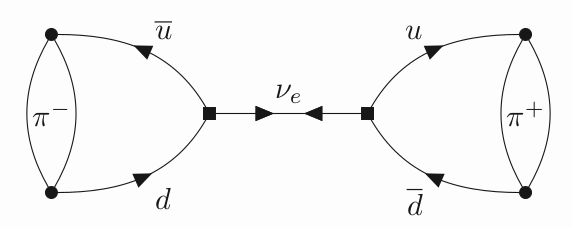
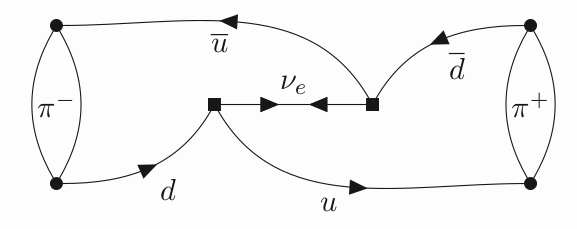
| (6) |
| (7) |
We denote the time slices of the source and sink by and , respectively. The remaining two contractions are obtained by exchanging the locations of the weak current insertions () and Lorentz indices ().
To extract the desired matrix element we employ methods which have been successfully applied to other second-order electroweak processes on the lattice, including the neutrinoful double beta decay process [3] and kaon decays [6, 7, 8]. By inserting a sum over intermediate states into the bilocal matrix element of Eqn. (3) it can be shown that the analogous lattice correlation function has the asymptotic time dependence
| (8) |
for pions at rest, where is the size of the temporal integration window for the weak current insertions and is the source-sink separation. In deriving this formula we have assumed that the current insertions are kept sufficiently far from the pion source and sink that potential couplings to excited states may be safely neglected. At large one can extract the matrix element
| (9) |
from a linear fit to the dependence of Eqn. (8).
In the present context we expect the lowest energy intermediate states to consist of a purely leptonic state and a single pion state , which require special consideration. The state contributes a term to Eqn. (8) which grows exponentially as , while, for the state, the energy denominator becomes small, potentially contributing a term . The remaining tower of multi-hadron states have energies and thus will contribute terms to Eqn. (8) which are asymptotically linear at large .
3 Pilot Lattice Study of the Decay
We have performed a pilot calculation using 1000 independent gauge field configurations of the domain wall fermion (DWF) ensemble described in Ref. [9]. This ensemble has a lattice cutoff of GeV and a physical volume of , with an unphysically heavy quark mass corresponding to a pion mass of MeV. We use Coulomb gauge-fixed wall source propagators for the quarks, and a free overlap propagator with an infinite temporal extent for the neutrino. Since performing the full integration over the locations of both weak current insertions is prohibitively expensive, we follow the strategy employed in Refs. [6, 7, 8] and treat the weak current insertions asymmetrically: the operator at is fixed at the (spatial) origin while the operator at is integrated over the spatial directions. Improved methods which will be used in future lattice calculations are discussed in Section 4.
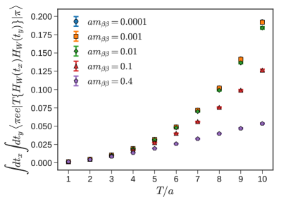
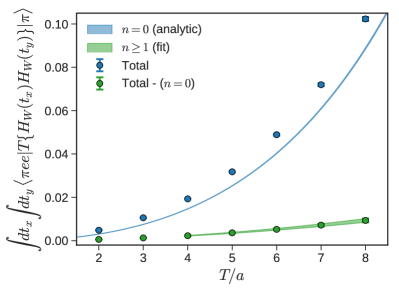
In the left panel of Figure 2 we plot the integrated bilocal matrix element described by Eqns. (3) and (8) as a function of , with the overall factor of removed, for a wide range of neutrino masses . For we observe the expected exponential divergence at large from the intermediate state, as well as the emergence of a consistent limit. We conclude that our calculation is insensitive to the precise choice of over the range of experimentally relevant neutrino masses. We have also performed the following analysis to extract the matrix element of Eqn. (9): we compute the matrix element describing the transition to the vacuum hadronic intermediate state — — and use this result to analytically construct and subtract the contribution from the intermediate state to Eqn. (8). After performing this subtraction, we then fit a quadratic function in to the remaining sum over higher intermediate states: from the quadratic term we recover the contribution from the state, and from the linear term we recover the sum over the remaining multi-hadron intermediate states. A preliminary analysis is summarized in the right panel of Figure 2 and in Table 1.
| () | |||
|---|---|---|---|
| -0.0082(15) | 1.0082(13) | 0.00009(26) |
In addition to extracting the matrix element Eqn. (9), lattice data for the quark mass dependence of the amplitude can also be matched to the known PT amplitude [10] to extract the next-to leading order low energy constant . First steps in this direction have been performed in Ref. [11], where it was reported that the amplitude is 24% and 9% smaller than the leading order PT prediction at MeV and MeV, respectively. Performing an explicit matching using our results with data at additional pion masses will be the subject of a future study.
4 Exact Treatment of the Neutrino Propagator
Lattice QCD calculations of many-body systems are known to suffer from signal-to-noise problems.
In anticipation of future calculations with baryonic and nuclear initial and final states, where we expect such signal-to-noise problems to enter, we have explored methods for performing an exact integration of the matrix element (3) over the spacetime locations of both current insertions; naively one expects an reduction in the statistical error from making use of the full lattice volume compared to the single sum method of our pilot study. We have also explored directly using the (Euclidean) infinite volume, continuum scalar propagator with a Gaussian UV cutoff for the neutrino,
| (10) |
which we expect to reduce finite volume effects compared to using a lattice propagator. Here the UV cutoff is required to render the matrix element of Eqn. (3) finite since the double integration will include contributions where . We choose , where is the lattice spacing, since this choice automatically enforces the removal of the UV cutoff in the continuum limit of the lattice calculation.
Implementing the double sum is more difficult, since an explicit double integration is prohibitively expensive even for a modestly-sized lattice calculation running on state-of-the-art computational resources. Fortunately, the translational invariance of the neutrino propagator can be exploited to reduce this to using the convolution theorem
| (11) |
and the fast Fourier transform (FFT). For the type 1 diagram, which factors into a product of traces involving only propagators to or propagators to , the contractions naturally take the form of Eqn. (11). For the type 2 diagram, which mixes and , we compute the convolutions of individual spin-color components and reconstruct the trace when we perform the final integration over .
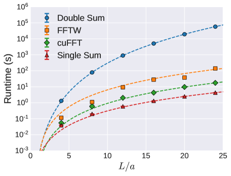
In the discrete lattice theory translational invariance implies that the neutrino propagator has a block Toeplitz matrix structure, and algorithms for performing block Toeplitz matrix-vector products via FFTs are well known in the literature. We have chosen to implement an algorithm described in Ref. [12], which performs the convolution and sum over Lorentz indices at the cost of three one-dimensional FFTs of size for a lattice of spatial size . In Figure 3 we benchmark the performance of this algorithm against an explicit double integration, as well as the single integration method used in our pilot study. Runtimes are shown for computing the type 2 contractions integrated over the spatial directions for a single, fixed time ordering of the weak current insertions. We also compare the performance of the OpenMP-threaded FFTW library running on a single Intel Xeon CPU to the performance of the cuFFT library running on an Nvidia GTX 1080 Ti GPU. We find that this strategy is effective in reducing the cost of the double summation to the point that it is feasible for realistic lattice volumes on existing computational resources. We also note a significant performance improvement for the GPU relative to the CPU as the lattice volume grows since large batches of FFTs can be computed in parallel.
5 Conclusions
We have performed an exploratory lattice QCD calculation of the transition amplitude on a domain wall fermion ensemble, and developed substantially improved methods applicable to general decay amplitudes. We are currently using these methods to compute the amplitude on domain wall fermion ensembles [13] at multiple pion masses, and including short-distance contributions [4] as well as the long-distance contributions described in this work. Analyzing these results and matching them to PT, as well as extending our calculations to include baryonic and nuclear initial and final states, will be the subject of future studies.
6 Acknowledgments
The authors thank N. Christ, X. Feng, R. Mawhinney, and A. Pochinsky for helpful discussions which have contributed to this work. W.D. and D.M. are partially supported by the U.S. Department of Energy through Early Career Research Award No. de-sc0010495 and Grant No. de-sc0011090, and by the SciDAC4 Grant No. de-sc0018121. Calculations were performed on the Blue Gene/Q supercomputer at Brookhaven National Lab.
References
- [1] A. Gando et al., “Search for Majorana Neutrinos Near the Inverted Mass Hierarchy Region with KamLAND-Zen”, Phys. Rev. Lett. 117, (2016) 082503.
- [2] A. Giuliani et al., “Neutrinoless Double-Beta Decay”, Adv. High Energy Phys. (2012) 857016.
- [3] B. Tiburzi et al., “Double- Decay Matrix Elements from Lattice Quantum Chromodynamics”, Phys. Rev. D 96 (2017) 054505.
- [4] A. Nicholson et al., “Heavy Physics Contributions to Neutrinoless Double Beta Decay from QCD”, Phys. Rev. Lett. 121, (2018) 172501.
- [5] S.M. Bilenky et al., “Neutrinoless Double-Beta Decay: A Probe of Physics Beyond the Standard Model”, Int. J Mod. Phys. A 30, (2015) 1530001.
- [6] Z. Bai et al., “ Decay Amplitude from Lattice QCD”, Phys. Rev. D 98 (2018) 074509.
- [7] Z. Bai et al, “ Mass Difference from Lattice QCD”, Phys. Rev.Lett. 113, (2014) 112003.
- [8] N.H. Christ et al., “Computing the Long-Distance Contributions to ”, PoS Lattice2015 (2016) 342.
- [9] C. Allton et al., “2+1 Flavor Domain Wall QCD on a Lattice: Light Meson Spectroscopy with ”, Phys. Rev. D 76 (2007) 014504.
- [10] V. Cirigliano et al., “Neutrinoless Double- Decay in Effective Field Theory: the Light-Majorana Neutrino-Exchange Mechanism”, Phys .Rev. C 97, (2018) 065501.
- [11] X. Feng et al., “Light-Neutrino Exchange and Long-Distance Contributions to Decays: An Exploratory Study on ”, arXiv:1809.10511 (2018).
- [12] B.E. Barrowes et al., “Fast Algorithm for Matrix-Vector Multiply of Asymmetric Multilevel Block-Toeplitz Matrices in 3-D Scattering”, Microwave Opt. Technol. Lett. 31: (2001) 28-32.
- [13] C. Allton et al., “Physical Results from 2+1 Flavor Domain Wall QCD and Chiral Perturbation Theory”, Phys. Rev. D 78, (2009) 114509.