Wavelet Based Dictionaries for Dimensionality Reduction of ECG Signals

Abstract

Dimensionality reduction of ECG signals is considered within the framework of sparse representation. The approach constructs the signal model by selecting elementary components from a redundant dictionary via a greedy strategy. The proposed wavelet dictionaries are built from the multiresolution scheme, but translating the prototypes within a shorter step than that corresponding to the wavelet basis. The reduced representation of the signal is shown to be suitable for compression at low level distortion. In that regard, compression results are superior to previously reported benchmarks on the MIT-BIH Arrhythmia data set.

1 Introduction

Electrocardiography (ECG) is the process of recording the electrical activity of the heart over a period of time. The overall goal of the test is to obtain information about the structure and function of that organ. Dimensionality reduction of ECG signals is relevant to techniques for analysis and classification of this type of data. Such techniques are subject of ongoing research [1, 2, 3, 4, 5, 6, 7, 8, 9], which includes methodologies based on the theory of compressive sensing [10, 11, 12, 13, 14].

Compressive sensing enhances the concept of sparsity by associating it to a new framework for digitalization [15, 16]. Producing sparse representation of ECG signals is the central aim of the present work. This implies to represent an ECG record as superposition of as few elementary components as possible. The same goal was traditionally accomplished by disregarding the least significant terms in the wavelet transform of the signal [17]. However, as shown in this work, much less elementary components are necessary if they are selected from a redundant wavelet dictionary rather than from a wavelet basis. This allows us to project an ECG record onto a subspace of lower dimensionality, in comparison to the dimension of the signal, and still reconstruct the record at low level distortion.

The main contributions of the paper are listed below:

• A number of wavelets dictionaries, based on existing families of wavelet bases, are developed.

• Each dictionary is shown to render much higher levels of sparsity for representing ECG signals than the corresponding basis. The tests are performed on the MIT-BIH Arrhythmia data set consisting of 48 records each of which of 30 min length.

• The metric of local sparsity is shown to be relevant to the detection of non-stationary noise or significant distortion in the patters of an ECG record.

• A strategy for storing the reduced representation of an ECG signal is considered. The resulting file is shown to render higher compression ratio than previously reported results within the state of the art for the same data set.

• MATLAB software for constructing the dictionaries, as well as for reproducing results, has been made available on a dedicated website [18].

The paper is organized as follows: Sec. 2 presents all the elements to build the proposed model for piecewise dimensionality reduction of an ECG record. Sec. 3 describes a strategy to encode the reduced representation of the signal. Sec. 4 presents and discusses numerical results. The conclusions are summarized in Sec. 5.

2 Piecewise ECG signal model

Assuming that an ECG record is given as an array $\mathbf{f}$ of dimension $N$, we divide the signal into $Q$ disjoint segments $\mathbf{f}_{q}\in\mathbb{R}^{N_{b}},\,q=1,\ldots,Q$ and construct an approximation $\mathbf{f}_{q}^{k_{q}}$ for each segment as the $k_{q}$-term ‘atomic decomposition’

$$\mathbf{f}_{q}^{k_{q}}=\sum_{n=1}^{k_{q}}c_{q}(n)\mathbf{d}_{\ell^{q}_{n}},$$ (1)

where the elements $\mathbf{d}_{\ell^{q}_{n}}$, called ‘atoms’, are chosen from a redundant dictionary ${\cal D}=\{\mathbf{d}_{n},\in\mathbb{R}^{N_{b}},\|\mathbf{d}_{n}\|=1\}$ through a greedy pursuit strategy. Here for the selection process we adopt the Optimized Orthogonal Matching Pursuit (OOMP) method [19, 20] which is stepwise optimal in the sense of minimizing the residual norm $\|\mathbf{f}_{q}-\mathbf{f}_{q}^{k_{q}}\|$ at each iteration. The algorithm evolves by selecting the atoms one by one as described next.

2.1 The OOMP Method

Since ECG records are normally superimposed to a smooth background, we initialize the OOMP algorithm by assuming that the constant atom $\mathbf{d}_{1}$ is always one of the elements in (1). Hence, for each $q$ we set $k_{q}=0$, $\Gamma_{q}=\emptyset$, $\ell_{1}^{q}=1$, and $\mathbf{w}_{1}^{q}=\mathbf{b}_{1}^{1,q}=\mathbf{d}_{1}$. Accordingly $\mathbf{f}_{q}^{1}=\mathbf{d}_{1}\langle\mathbf{f}_{q},\mathbf{d}_{1}\rangle$ (where $\langle\cdot,\cdot\rangle$ indicates the Euclidean inner product), and $\mathbf{r}_{q}^{1}=\mathbf{f}_{q}-\mathbf{f}_{q}^{1}$.

From the above initialization the OOMP approach for selecting from ${\cal D}$ the elements $\mathbf{d}_{\ell^{q}_{n}},\,n=2,\ldots,k_{q}$ in (1), and calculating the corresponding coefficients $c_{q}(n),\,\,n=1,\ldots,k_{q}$, iterates as follows.

• Upgrade the set $\Gamma_{q}\leftarrow\Gamma_{q}\cup\ell_{k_{q}+1}^{q}$, increase $k_{q}\leftarrow k_{q}+1$, and select the index of a new atom for the approximation as

  $$\ell_{k_{q}+1}^{q}=\operatorname*{arg\,max}_{\begin{subarray}{c}n=1,\ldots,M\\ n\notin\Gamma_{q}\end{subarray}}\frac{|\langle\mathbf{d}_{n},\mathbf{r}_{q}^{k_{q}}\rangle|^{2}}{1-\sum_{i=1}^{k_{q}}|\langle\mathbf{d}_{n},\tilde{\mathbf{w}}_{i}^{q}\rangle|^{2}},$$ (2)

  with $\tilde{\mathbf{w}}_{i}^{q}=\frac{\mathbf{w}_{i}^{q}}{\|\mathbf{w}_{i}^{q}\|}$.

• Orthogonalization step. Compute the corresponding new vector $\mathbf{w}_{k_{q}+1}^{q}$ as

  $$\begin{split}\mathbf{w}_{k_{q}+1}^{q}=\mathbf{d}_{\ell_{k_{q}+1}^{q}}-\sum_{n=1}^{k_{q}}\frac{\mathbf{w}_{n}^{q}}{\|\mathbf{w}_{n}^{q}\|^{2}}\langle\mathbf{w}_{n}^{q},\mathbf{d}_{\ell_{k_{q}+1}^{q}}\rangle\end{split}$$ (3)

  including, for numerical accuracy, the re-orthogonalization step:

  $$\mathbf{w}_{k_{q}+1}^{q}\leftarrow\mathbf{w}_{k_{q}+1}^{q}-\sum_{n=1}^{k_{q}}\frac{\mathbf{w}_{n}^{q}}{\|\mathbf{w}_{n}^{q}\|^{2}}\langle\mathbf{w}_{n}^{q},\mathbf{w}_{k_{q}+1}^{q}\rangle.$$ (4)

• Biorthogonalization step. For $n=1,\ldots,k_{q}$ upgrade vectors $\mathbf{b}_{n}^{k_{q},q}$ as

  $$\begin{split}\mathbf{b}_{n}^{{k_{q}}+1,q}&=\mathbf{b}_{n}^{{k_{q}},q}-\mathbf{b}_{k_{q}+1}^{{k_{q}}+1,q}\langle\mathbf{d}_{\ell_{{k_{q}}+1}^{q}},\mathbf{b}_{n}^{k_{q}+1,q}\rangle,\\ \mathbf{b}_{k_{q}+1}^{k_{q}+1,q}&=\frac{\mathbf{w}_{k_{q}+1}^{q}}{\|\mathbf{w}_{k_{q}+1}^{q}\|^{2}}.\end{split}$$ (5)

• Calculate

  $$\mathbf{r}_{q}^{k_{q}+1} = \mathbf{r}_{q}^{k_{q}}-\langle\mathbf{w}_{k_{q}+1}^{q},\mathbf{f}_{q}\rangle\frac{\mathbf{w}_{k_{q}+1}^{q}}{\|\mathbf{w}_{k_{q}+1}^{q}\|^{2}}.$$ (6)

• If for a given $\rho$ the condition $\|\mathbf{r}_{q}^{k_{q}+1}\|<\rho$ has been met compute the coefficients $c_{q}(n)=\langle\mathbf{b}_{n}^{k_{q}+1},\mathbf{f}_{q}\rangle,\,n=1,\ldots,k_{q}+1$ to write the approximation $\mathbf{f}_{q}^{k_{q}}$ of $\mathbf{f}_{q}$ as in (1). Otherwise repeat steps 1) - 5).

Once all the segments $\mathbf{f}_{q}$ have been approximated, the approximation of the whole signal is obtained by assembling the approximation of the segments as $\mathbf{f}^{\rm{r}}=\hat{\operatorname{J}}_{q=1}^{Q}\mathbf{f}_{q}^{k_{q}}$, where $\hat{\operatorname{J}}$ is the concatenation operation.

The complexity of the method, dominated by the selection of atoms, is O($KN_{b}M$) with $K=\sum_{q=1}^{Q}k_{q}.$

A suitable model for dimensionality reduction of the signal must involve significantly fewer atoms in their atomic decomposition than the dimension of the signal. The success in achieving such a goal depends on the dictionary being used. Next we discuss wavelet dictionaries which are fit for the purpose.

2.2 Wavelet Based Dictionaries

The proposed wavelet dictionaries are inspired on the construction of dictionaries for Cardinal Spline Spaces (CSS) as discussed in previous works [21, 22, 23]. Let us denote $V_{j},j\geq 0$ to the CSS of order $m$ with simple knots at the equidistant partition of the interval $[c,d]$ having distance $2^{-j}$ between two adjacent knots. A basis for $V_{j}$ arises from the restriction of the functions

$$\phi_{j,k}(x):=2^{j/2}\phi(2^{j}x-k),\,k\in\mathbb{Z}$$ (7)

to the interval $[c,d]$, which we expressed as $2^{j/2}\phi(2^{j}x-k)|_{[c,d]}$. The function $\phi(x)\equiv\phi_{0,0}(x)$ is called scaling function. For a CSS $\phi(x)$ is the cardinal B-spline of order $m$ associated with the uniform simple knot sequence $0,1,\dots,m$ [24]

$$\phi(x)=\frac{1}{m!}\sum_{i=0}^{m}(-1)^{i}\binom{m}{i}(x-i)^{m-1}_{+},$$ (8)

where $(x-i)^{m-1}_{+}$ is equal to $(x-i)^{m-1}$ if $x-i>0$ and 0 otherwise.

The complementary wavelet subspace $W_{j}$ on $[c,d]$ is constructed in order to fulfil

$$V_{j+1}=V_{j}\oplus W_{j},\ j\in\mathbb{Z}^{+},$$ (9)

where $\oplus$ indicates the direct sum, i.e. $V_{j}\cap W_{j}=\{0\}$. Hence,

$$V_{j+1}=V_{0}\oplus W_{0}\oplus W_{1}\oplus\cdots W_{j}.$$ (10)

For a given value of $j$ a wavelet basis for $W_{j}$ arises as

$$\psi_{j,k}(x)=2^{j/2}\psi(2^{j}x-k)|_{[c,d]},\,k\in\mathbb{Z}$$ (11)

and the elimination of some redundancy introduced by the cutting process at the borders of the interval. Different constructions of mother wavelets $\psi\equiv\psi_{0,0}$ give rise to different wavelet bases.

Within the multi-resolution framework, dictionaries for a CSS are simply constructed from the result asserting that if for $l\in\mathbb{Z}^{+}$

$${\cal W}_{j,l}=\{2^{j/2}\psi(2^{j}x-\frac{k}{2^{l}})|_{[c,d]},\,k\in\mathbb{Z}\},$$ (12)

then [22]

$${\mbox{\rm{span}}}\{{\cal W}_{j,l}\}=V_{{j+l}}.$$ (13)

This result facilitates a tool for designing dictionaries of wavelets of different support spanning the same CSS. A multi-resolution-like dictionary ${\cal D}_{j,l}$ spanning $V_{{j}}$ is constructed as

$${\cal D}_{j,\ell}={\cal V}_{0,l}\cup{\cal W}_{0,l}\cup{\cal W}_{1,l}\cup\cdots\cup{\cal W}_{j-l,l},$$ (14)

with

$${\cal V}_{0,l}=\{\phi(x-\frac{k}{2^{l}})|_{[c,d]},\,k\in\mathbb{Z}\}.$$ (15)

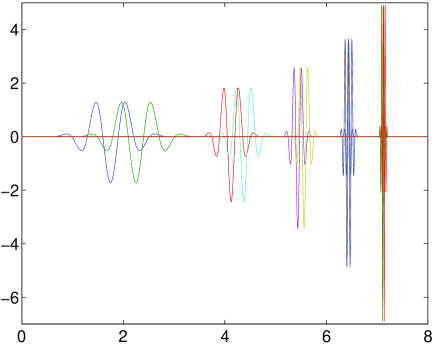
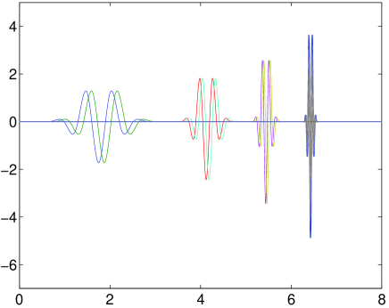
Figure 1: Wavelet functions taken from a basis for a CSS (left graph) and from a dictionary spanning the same CSS (right graph).

The top graph of Fig. 1 shows consecutive wavelets in a cubic Chui-Wang4 [25] wavelet basis and consecutive wavelets in a dictionary for the same CSS. Notice that the wavelet functions at the finest scale in the dictionary are broader than those at the finest scale in the basis.

For the sake of comparison we have built dictionaries for the following wavelet families.

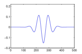
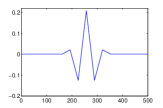
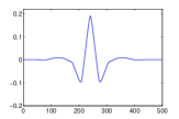
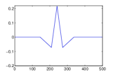
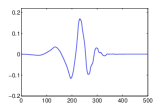
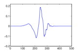
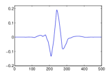
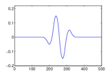
Figure 2: Wavelet prototypes. From left top to right bottom the graphs correspond to the families $\mathbf{CW4},$ $\mathbf{CW2},$ $\mathbf{CDF97},$ $\mathbf{CDF53},$ $\mathbf{Db4},$ $\mathbf{Coif},$ $\mathbf{Sym},$ and $\mathbf{Short3}$.

Semi-orthogonal spline wavelets were mentioned above. Their construction was proposed by C. Chui and J. Wang in [25]. Semi-orthogonal wavelets, also called prewavelets, are not orthogonal if the wavelets are at the same scale level, but orthogonality of wavelets at the different levels is preserved. Here we consider the cubic and linear cases, which are indicated as $\mathbf{CW4}$ and $\mathbf{CW2}$ respectively. The wavelet prototypes corresponding to this family are given the 1st and 2nd graphs in the 1st row Fig. 2.

Cohen-Daubechies-Feauveau biorthogonal wavelets were built in [26]. In this case both primal and dual wavelets have compact support. Wavelets from this family with 9 and 7 taps filters (CDF97) and with 5 and 3 taps filters (CDF53) are used in the JPEG2000 compression standard. The corresponding prototypes are given in the 3rd and 4th graphs in the 1st row of Fig. 2.

Daubechies wavelets were built by I. Daubechies as first orthonormal compactly supported continuous wavelets in [27]. They have the shortest possible support for the given number of vanishing moments and they have extremal phase. Here we consider the four vanishing moments and indicate it as Db4. This wavelet prototype is displayed in the 1st graph of the 2nd row of Fig. 2.

Coiflets were suggested by R. Coifman as orthonormal wavelet systems with vanishing moments for both scaling functions and wavelets. They were first constructed by I. Daubechies in [28]. We consider two vanishing moments used exact values of scaling and wavelet parameters from [29] and indicate the family as Coif. The mother wavelet is displayed in the 2nd graph in the 2nd row of Fig. 2.

Symlets are modified version of Daubechies wavelets. They have also the shortest possible support for the given number of vanishing moments, see [28]. We consider four vanishing moments. The prototype wavelet for the family Sym is given in the 3rd graph in the 2nd row of Fig. 2.

Spline wavelets with short support are obtained if the local support of dual wavelets is not required. They were designed in [30, 31]. Here we consider quadratic splines and indicate them as $\mathbf{Short3}$. The prototype for this family is plotted in last graph of the 2nd row of Fig. 2.

In the discrete case dictionaries can be constructed in a very simple manner: A redundant dictionary for the Euclidean space $\mathbb{R}^{N}$ is simply any set of normalized vectors $\{\mathbf{d}_{i}\in\mathbb{R}^{N},\,\|\mathbf{d}_{i}\|=1\}_{i=1}^{M}$ such that $N$ of them are linearly independent and $M>N$. Inspired by the results for CSS we construct a dictionary for $\mathbb{R}^{N}$ simply by discretization of the functions in the wavelet dictionary. As already mentioned, ECG signals are commonly superimposed to a smooth background, hence we enrich a wavelet dictionary adding a few low frequency components from a discrete cosine basis. Thus the whole dictionary we consider is built as ${\cal D}={\cal D}^{\rm{C}}\cup{\cal D}^{\rm{W}}$, with ${\cal D}^{\rm{W}}$ a discrete wavelet basis (or dictionary) for $\mathbb{R}^{N_{b}}$ and

$${\cal D}^{\rm{C}} = \{w_{c}(n)\cos{\frac{{\pi(2i-1)(n-1)}}{2M}},i=1,\ldots,N_{b}\}_{n=1}^{M},$$

where each $w_{c}(n)$ is a normalization constant. For the numerical tests we fix $M=10$ for ${\cal D}^{\rm{C}}$ and for ${\cal D}^{\rm{W}}$ we consider different wavelet dictionaries, all obtained from the aboved mentioned wavelet bases.

3 Encoding the signal model

For the reduced representation of the signal (1) to be suitable for storage and transmission purposes it is necessary to encode it within a small file in relation to the size of the original record. For this end, firstly the absolute value coefficients $|c_{q}(n)|,\,n=1\ldots,k_{q},\,q=1,\ldots,Q,$ are converted into integers as follows:

$$c^{\Delta}_{q}(n)=\lfloor\frac{|c_{q}(n)|}{\Delta}+\frac{1}{2}\rfloor,$$ (16)

where $\lfloor x\rfloor$ indicates the largest integer number smaller or equal to $x$ and $\Delta$ is the quantization parameter. The signs of the coefficients, represented as $\mathbf{s}_{q},\,q=1,\ldots,Q$, are encoded separately using a binary alphabet. For creating the strings of numbers to encode the the signal model we proceed as in [32, 33].

The indices of the atoms in the atomic decompositions of each block $\mathbf{f}_{q}$ are first sorted in ascending order $\ell_{i}^{q}\rightarrow\tilde{\ell}_{i}^{q},\,i=1,\ldots,k_{q}$, which guarantees that, for each $q$ value, $\tilde{\ell}_{i}^{q}<\tilde{\ell}_{i+1}^{q},\,i=1,\ldots,k_{q}-1$. The order of the indices induces order in the unsigned coefficients, $\mathbf{c}^{\Delta}_{q}\rightarrow\mathbf{\tilde{c}}^{\Delta}_{q}$ and in the corresponding signs $\mathbf{s}_{q}\rightarrow\mathbf{\tilde{s}}_{q}$. The ordered indices are stored as smaller positive numbers by taking differences between two consecutive values. By defining $\delta^{q}_{i}=\tilde{\ell}^{q}_{i}-\tilde{\ell}^{q}_{i-1},\,i=2,\ldots,k_{q}$ the follow string stores the indices for block $q$ with unique recovery ${\tilde{\ell}^{q}_{1},\delta^{q}_{2},\ldots,\delta^{q}_{k_{q}}}$. The number ‘0’ is then used to separate the string corresponding to different blocks and entropy code a long string, $st_{\rm{ind}}$, which is built as

$$st_{\rm{ind}}=[{\tilde{\ell}_{1}}^{1},\ldots,\delta^{1}_{k_{1}},0,{\tilde{\ell}_{1}}^{2},\ldots,\delta^{2}_{k_{2}},0,\cdots,{\tilde{\ell}_{1}}^{k_{Q}},\ldots,\delta^{Q}_{k_{Q}}].$$ (17)

The corresponding quantized magnitude of the coefficients are concatenated in the strings $st_{\rm{cf}}$ as follows:

$$st_{\rm{cf}}=[\tilde{c}^{\Delta}_{1}(1),\ldots,\tilde{c}^{\Delta}_{1}(k_{1}),\cdots,\tilde{c}^{\Delta}_{{k_{Q}}}(1),\ldots,\tilde{c}^{\Delta}_{{k_{Q}}}(k_{Q})].$$ (18)

Using ‘0’ to store a positive sign and ‘1’ to store negative one, the signs are placed in the string, $st_{\rm{sg}}$ as

$$st_{\rm{sg}}=[\tilde{s}_{1}(1),\ldots,\tilde{s}_{1}(k_{1}),\cdots,\tilde{s}_{{k_{Q}}}(1),\ldots,\tilde{s}_{{k_{Q}}}(k_{Q})].$$ (19)

4 Results

The numerical tests we present here use the full MIT-BIH Arrhythmia database [35] which contains 48 ECG records. Each of these records is of 30 min length, consisting of $N=650000$ 11-bit samples at a frequency of 360 Hz.

All our results have been obtained in the MATLAB environment using a notebook 2.9GHz dual core i7 3520M CPU and 4GB of memory.

4.1 Assessment Metrics

The quality of the signal approximation is assessed with respect to the $\mathrm{PRD}$ calculated as follows,

$$\mathrm{PRD}=\frac{\|\mathbf{f}-\mathbf{f}^{\rm{r}}\|}{\|\mathbf{f}\|}\times 100\%\quad$$ (20)

where, $\mathbf{f}$ is the original signal and $\mathbf{f}^{\rm{r}}$ is the signal reconstructed from the approximated segments. Since the $\mathrm{PRD}$ strongly depends on the background of the signal, the $\mathrm{PRDN}$ as defined below is also a relevant metric.

$$\mathrm{PRDN}=\frac{\|\mathbf{f}-\mathbf{f}^{\rm{r}}\|}{\|\mathbf{f}-\overline{\mathbf{f}}\|}\times 100\%,\quad$$ (21)

where, $\overline{\mathbf{f}}$ indicates the mean value of $\mathbf{f}$.

For a fixed value of $\mathrm{PRD}$ the sparsity of a representation is assessed by the sparsity ratio (SR)

$$\text{SR}=\frac{N}{K},$$ (22)

where $N$ is the total length of the signal and $K=\sum_{q=1}^{Q}k_{q},$ with $k_{q}$ the number of atoms in the atomic decomposition (1) of each segment of length $N_{b}$. For detection of nonstationary noise in patterns it is useful to define the measure of local sparsity $\mathrm{sr}(q)$ as follows:

$$\mathrm{sr}(q)=\frac{N_{b}}{k_{q}},\quad q=1,\ldots Q.$$ (23)

The compression performance depends of the size of the file storing the signal representation and is assessed by the Compression Ratio (CR) as given by

$$\text{CR}=\frac{{\text{Size of the uncompressed file}}}{{\text{Size of the compressed file}}}.$$ (24)

In the numerical tests below we use the notation $\mathrm{CR}$ to denote the compression ratio obtained when the string $st_{\rm{ind}},st_{\rm{cf}}$ and $st_{\rm{sg}}$ are stored in hierarchical data format [34], simply using the MATLAB instruction save. If a Huffman coding step is included the corresponding compression ratio is denoted as $\mathrm{CR}^{\bf{Hf}}$.

The quality score ($\mathrm{QS}$), reflecting the tradeoff between compression performance and reconstruction quality, is the ratio:

$$\mathrm{QS}=\frac{\mathrm{CR}}{\mathrm{PRD}}.$$ (25)

Since the $\mathrm{PRD}$ is a global quantity, in order to detect possible local changes in the visual quality of the recovered signal, we consider the local $\mathrm{PRD}$ as follows. Each signal is partitioned in $Q$ segments $\mathbf{f}_{q},\,q=1\ldots,Q$ of $N_{b}$ samples. The local $\mathrm{PRD}$ with respect to every segment in the partition is indicate as ${\mathrm{prd}}(q),\,q=1,\ldots Q$ and calculated as

$${\mathrm{prd}}(q)=\frac{\|\mathbf{f}_{q}-\mathbf{f}^{\rm{r}}_{q}\|}{\|\mathbf{f}_{q}\|}\times 100\%,\quad$$ (26)

where $\mathbf{f}^{\rm{r}}_{q}$ is the recovered portion of the signal corresponding to the segment $q$. In all the numerical test of the next section the OOMP approximation is stopped through a fixed value $\rho$ so as to achieve the same value of ${\mathrm{prd}}$ for all the segments in the records. Assuming that the target ${\mathrm{prd}}$ before quantization is ${\mathrm{prd}_{0}}$ we set $\rho={\mathrm{prd}_{0}}\|\mathbf{f}_{q}\|/100$.

4.2 Test I

The purpose of the first numerical tests is to demonstrate the significant gain in dimensionality reduction (high values of $\mathrm{SR}$) achieved if the component ${\cal D}^{\rm{W}}$ of the dictionary ${\cal D}$ is a wavelet dictionary instead of a wavelet basis. The wavelet basis arises using as translation parameter $b=1$ and the wavelet dictionary using a translation parameter $b=1/4$. A wavelet basis contains scales corresponding to the values $j=3,\ldots,8$ while the corresponding dictionary contains one less scale i.e. $j=3,\ldots,7$. The exact redundancy of the dictionary depends of the wavelet family but in all the cases is close to two. The records are approximated by partitioning the signal into $Q=1300$ segments of $N_{b}=500$ data points each.

The second column in Table 1 gives the mean value $\mathrm{SR}$, after quantization, with respect to the 48 records in the data set. The standard deviation is given in the 3rd column. The approximation with all the families is accomplished to obtain the same mean value of $\mathrm{PRD}$ ($\overline{\mathrm{PRD}}=53$). For this test the quantization parameter is fixed. For all the records and all the dictionaries $\Delta=35$. The 4th column gives the mean value $\mathrm{CR}$ and the fifth column the corresponding standard deviation. For further improvement in $\mathrm{CR}$ we have added an entropy coding step to represent the strings described in Sec. 3 at a fixed bit depth using Huffman coding. The implementation of the step is realized using the off-the-shelf MATLAB function Huff06 available on [36]. The corresponding outcomes, indicated as $\overline{\mathrm{CR}}^{\mathbf{Hf}}$, are given in the sixth column of Table  1. The 1st column lists the different wavelet families which are considered to build the dictionary ${\cal D}^{\rm{W}}$. The subscript B is used to indicate the wavelet basis and the subscript D to indicate the corresponding dictionary, i.e. $\mathbf{CDF97}_{\mathbf{B}}$ indicates the 9/7 Cohen-Daubechies-Feauveau biorthogonal wavelet basis and $\mathbf{CDF97}_{\mathbf{D}}$ the corresponding wavelet dictionary. For further of comparison the last row of the table gives the results produced when a Fast Wavelet Transform (FWT) is applied on the whole record, as proposed in [37].

Table 1: Mean values of $\mathrm{SR}$ and $\mathrm{CR}$ with respect to the 48 records in the MIT-BIH Arrhythmia database. In all the cases the reconstructed signals produce $\overline{\mathrm{PRD}}=53$.

${\cal D}^{\rm{W}}$	${\overline{\mathrm{SR}}}$	$\mathrm{std}$	${\overline{\mathrm{CR}}}$	$\mathrm{std}$	$\overline{\mathrm{CR}}^{\mathbf{Hf}}$	$\mathrm{std}$
$\mathbf{CW4}_{\mathbf{B}}$	10.13	2.42	11.72	3.14	16.70	3.78
$\mathbf{CW4}_{\mathbf{D}}$	16.62	4.13	13.31	3.51	17.80	4.40
$\mathbf{CW2}_{\mathbf{B}}$	11.34	2.91	12.08	3.48	17.78	4.34
$\mathbf{CW2}_{\mathbf{D}}$	16.76	4.95	13.91	4.04	18.37	5.25
$\mathbf{CDF97}_{\mathbf{B}}$	14.59	3.90	14.90	4.20	20.54	4.99
$\mathbf{CDF97}_{\mathbf{D}}$	20.60	5.79	16.13	4.57	21.26	5.82
$\mathbf{CDF53}_{\mathbf{B}}$	14.72	4.25	14.84	4.29	20.46	5.31
$\mathbf{CDF53}_{\mathbf{D}}$	20.18	6.36	16.02	4.88	21.04	6.27
$\mathbf{Db4}_{\mathbf{B}}$	12.81	3.28	13.49	3.63	18.81	4.46
$\mathbf{Db4}_{\mathbf{D}}$	17.88	4.94	14.24	4.05	18.97	5.15
$\mathbf{Coif}_{\mathbf{B}}$	11.50	2.99	12.66	3.47	17.41	4.29
$\mathbf{Coif}_{\mathbf{D}}$	15.27	4.57	12.58	3.68	16.73	4.74
$\mathbf{Sym}_{\mathbf{B}}$	12.83	3.30	13.65	3.68	18.96	4.47
$\mathbf{Sym}_{\mathbf{D}}$	18.51	5.26	14.70	4.22	19.26	5.77
$\mathbf{Short3}_{\mathbf{B}}$	12.78	3.18	15.09	4.31	19.68	4.59
$\mathbf{Short3}_{\mathbf{D}}$	19.84	5.25	16.00	4.24	20.95	5.46
FWT[37]	11.22	1.75	23.17	6.57	26.34	6.99

As seen in Table 1 the best results in relation to dimensionality reduction (largest values of ${\overline{\mathrm{SR}}}$) are for $\mathbf{CDF97}_{\mathbf{D}},\mathbf{CDF53}_{\mathbf{D}}$ and $\mathbf{Short3}_{\mathbf{D}}$ and all the wavelet bases perform poorly in comparison to the dictionaries. The difference in ${\overline{\mathrm{CR}}}$ is not so pronounced though. This is because, in spite of the fact that the approximation using a dictionary involves much less elementary components in the signal decomposition, the dispersion of indices corresponding to the atoms in the decomposition is larger if using a dictionary. Notice that, as far as compression is concerned using a FWT to transform the whole signal is more effective than a piecewise transformation. This is true not only in terms of the achieved ${\overline{\mathrm{CR}}}$ but also in regard to computational time (the approach advanced in [37] is very fast). Contrarily, as indicated by the values of ${\overline{\mathrm{SR}}}$ in Table 1 the method in [37] is not as effective for dimensionality reduction as it is for compression. However, dimensionality reduction is relevant in its own right to methodologies for classification and recognition tasks[38, 39].

Table 2: Performance metrics for each of the 48 records in the MIT-BIH Arrhythmia database listed in the first column.

Rec	$\mathrm{PRD}$	$\mathrm{SR}$	$\mathrm{CR}^{\mathbf{Hf}}$	$\mathrm{QS}$	$\mathrm{PRDN}$
100	0.51	27.19	28.27	55.75	12.64
101	0.51	25.39	25.89	50.82	9.45
102	0.51	24.43	24.74	48.27	13.13
103	0.52	21.93	22.06	42.73	7.86
104	0.53	19.00	19.52	37.21	10.27
105	0.53	17.37	18.15	34.22	6.43
106	0.53	18.63	18.87	35.97	7.07
107	0.55	12.64	12.66	23.01	3.18
108	0.52	21.13	22.74	43.52	8.51
109	0.52	19.32	19.42	37.05	5.16
111	0.51	23.22	24.32	47.45	9.90
112	0.53	22.72	24.47	46.18	10.20
113	0.52	20.21	19.80	38.18	6.26
114	0.50	32.21	33.13	66.17	14.52
115	0.53	20.18	20.52	38.98	6.73
116	0.58	12.33	12.90	22.10	3.72
117	0.52	27.31	28.82	55.27	9.33
118	0.59	11.06	12.51	21.22	5.90
119	0.56	16.15	16.50	29.78	4.44
121	0.51	33.27	33.61	66.10	7.29
122	0.56	16.42	17.62	31.80	6.50
123	0.53	21.94	22.93	43.11	7.94
124	0.53	23.28	23.09	43.92	4.94
200	0.53	15.56	16.69	31.33	7.05
201	0.49	34.72	35.05	71.66	12.52

Rec	$\mathrm{PRD}$	$\mathrm{SR}$	$\mathrm{CR}^{\mathbf{Hf}}$	$\mathrm{QS}$	$\mathrm{PRDN}$
202	0.51	26.24	26.28	51.87	8.44
203	0.55	12.75	13.86	25.14	5.54
205	0.51	25.25	26.83	52.54	12.50
207	0.51	25.93	25.66	50.80	7.08
208	0.54	15.09	15.69	29.16	5.55
209	0.54	15.65	16.83	31.40	9.92
210	0.51	23.84	24.62	48.18	9.72
212	0.56	12.12	13.56	24.40	8.35
213	0.56	11.71	12.06	21.71	4.09
214	0.52	19.22	19.15	36.59	5.54
215	0.55	14.07	15.34	28.20	9.60
217	0.53	16.86	16.47	31.06	4.30
219	0.54	18.06	18.00	33.69	4.43
220	0.53	19.18	19.65	37.07	7.65
221	0.52	22.73	23.00	44.69	8.50
222	0.51	26.52	27.53	54.42	13.53
223	0.53	18.56	18.70	35.09	6.06
228	0.52	18.97	20.31	38.91	7.53
230	0.52	19.12	19.47	37.29	7.30
231	0.51	25.67	26.20	51.84	9.23
232	0.50	29.72	31.59	63.83	14.91
233	0.54	14.26	14.81	27.43	4.96
234	0.52	19.81	20.50	39.28	7.68
mean	0.53	20.60	21.26	40.76	7.99
std	0.02	5.79	5.82	12.47	2.92

For further information in Table 2 we provide the figures of the evaluation metrics for each of the 48 records in the dataset. The 2nd column of Table 2 shows the values of $\mathrm{PRD}$ for the records listed in the 1st column. The 3rd column shows the values of $\mathrm{SR}$ after quantization. The $\mathrm{CR}^{\mathbf{Hf}}$ is given in the 4th column and the corresponding $\mathrm{QS}$ in the 5th column. The last column corresponds to the values of $\mathrm{PRDN}$. All the results are obtained using the dictionary $\mathbf{CDF97}_{\mathbf{D}}$. The average time for producing Table 2 is 30 s per record.

Fig. 3 depicts the approximation and raw data (indistinguishable in the scale of the graphs) of 2000 points in the records 107 and 116.

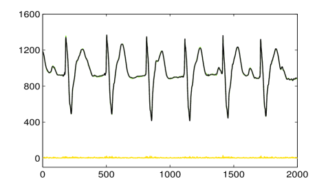
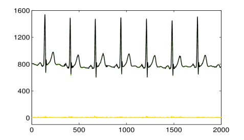
Figure 3: The waveforms in the graphs are the raw data and the approximations corresponding to 2000 points in the records 107 (left) and 116 (right). The bottom lines represent the absolute value of the difference between the data and the approximation.

4.3 Test II

In this test we compare compression results with previously reported benchmarks on the MIT-BIH Arrhythmia database. Since the PRD strongly depends on the baseline in the ECG record, when using the relation CR vs PRD for comparison one needs to be able to confirm that the values of PRD reported in previous work either, do not include any subtraction of baseline, or the subtracted value is also reported. From the information given in the papers we are comparing with (the relation between the values of PRD and PRDN) we can guarantee that the results correspond to the same database [35] and without any subtraction of baseline. In the range $[0.31\;0.67]$ the comparison is realized with the classical benchmark [40]. This method is based on peak detection to perform the Discrete Cosine Transform (DCT) between consecutive peaks and Huffman encoding for lossless compression. In the range $[0.80\;1.71]$ the comparison is with the methods in [41] and [42]. Both these methods are based on Adaptive Fourier Decomposition (AFD) and overperform those in [40] and [43] for values of $\mathrm{PRD}$ in the range being considered. In [42] the lossless compression is realized using Huffman coding while [41] applies symbol substitution. Comparisons are also produced with the results arising when a FWT is applied on the full record [37].

Table 3 compares CRs obtain with $\mathbf{CDF97}_{\mathbf{D}}$ and $\mathbf{CDF53}_{\mathbf{D}}$ for values of $\mathrm{PRD}$ in the range $[0.31\;0.81]$, Table 4 for values in the range $[0.91\;1.06]$, and Table 5 in the range $[0.14\;1.71]$. The last two rows in all the tables give the values of the quantization parameter, $\Delta$, and the approximation parameter ${\mathrm{prd}_{0}}$. These parameters are set in order to reproduce the same values of $\mathrm{PRD}$ as in the publications we are comparing with.

Table 3: Comparison between the average compression performance of the proposed method and the methods in [40], [41], [42] and [37], for values of ${\overline{\mathrm{PRD}}}$ in the range [0.31   0,81].

${\overline{\mathrm{PRD}}}$	0.81	0.80	0.67	0.48	0.31
${\overline{\mathrm{CR}}}$[40]			11.30	9.28	6.22
${\overline{\mathrm{CR}}}$[41]		18.00
${\overline{\mathrm{CR}}}$[42]	16.85
${\overline{\mathrm{CR}}}$[37]	33.32	33.05	27.79	19.84	10.59
$\overline{\mathrm{CR}}^{\mathbf{Hf}}$[37]	36.54	36.26	31.01	23.09	15.00
${\overline{\mathrm{CR}}}\,\,\,\,\,\,\mathbf{CDF97}_{\mathbf{D}}$	24.03	23.81	20.52	14.79	9.37
$\overline{\mathrm{CR}}^{\mathbf{Hf}}\,\mathbf{CDF97}_{\mathbf{D}}$	31.64	31.07	26.71	19.59	12.50
${\overline{\mathrm{CR}}}\,\,\,\,\,\,\mathbf{CDF53}_{\mathbf{D}}$	24.76	24.50	20.67	14.67	8.89
$\overline{\mathrm{CR}}^{\mathbf{Hf}}\,\mathbf{CDF53}_{\mathbf{D}}$	32.59	31.93	26.01	19.25	11.93
${\mathrm{prd}_{0}}$	0.750	0.740	0.645	0.435	0.275
$\Delta$	60	60	40	30	16

Table 4: Comparison between the average compression performance of the proposed method and the methods in [41], [42], [43] and [37], for values of ${\overline{\mathrm{PRD}}}$ in the range $[0.91\;1.06]$.

${\overline{\mathrm{PRD}}}$	1.06	1.05	1.03	0.94	0.91
${\overline{\mathrm{CR}}}$[41]		25.667			22.27
${\overline{\mathrm{CR}}}$[42]			22.80	20.38
${\overline{\mathrm{CR}}}$[43]	18.59
${\overline{\mathrm{CR}}}$[37]	41.31	41.24	41.00	38.52	37.68
$\overline{\mathrm{CR}}^{\mathbf{Hf}}$[37]	44.42	44.23	44.04	41.93	41.08
${\overline{\mathrm{CR}}}\,\,\,\,\,\,\mathbf{CDF97}_{\mathbf{D}}$	30.36	30.12	29.44	27.29	26.27
$\overline{\mathrm{CR}}^{\mathbf{Hf}}\,\mathbf{CDF97}_{\mathbf{D}}$	40.25	39.96	39.11	35.94	34.42
${\overline{\mathrm{CR}}}\,\,\,\,\,\,\mathbf{CDF53}_{\mathbf{D}}$	31.93	31.66	30.84	28.46	27.28
$\overline{\mathrm{CR}}^{\mathbf{Hf}}\,\mathbf{CDF53}_{\mathbf{D}}$	42.73	42.39	41.40	37.81	35.70
$\Delta$	100	100	100	80	80
${\mathrm{prd}_{0}}$	0.940	0.930	0.900	0.850	0.805

Table 5: Comparison between the average compression performance of the proposed method and the methods in [41], [42], and [37] for values of ${\overline{\mathrm{PRD}}}$ in the range $[1.14\;1.71]$.

${\overline{\mathrm{PRD}}}$	1.71	1.47	1.29	1.18	1.14
${\overline{\mathrm{CR}}}$[41]	38.46	33.85		28.21
${\overline{\mathrm{CR}}}$[42]	42.27	3.53	30.21		25.99
${\overline{\mathrm{CR}}}$[37]	62.48	56.78	49.60	47.04	45.75
$\overline{\mathrm{CR}}^{\mathbf{Hf}}$[37]	63.92	58.59	52.19	49.59	48.47
${\overline{\mathrm{CR}}}\,\,\,\,\,\,\mathbf{CDF97}_{\mathbf{D}}$	52.01	43.83	37.63	33.88	32.69
$\overline{\mathrm{CR}}^{\mathbf{Hf}}\,\mathbf{CDF97}_{\mathbf{D}}$	66.99	56.44	48.77	44.45	42.98
${\overline{\mathrm{CR}}}\,\,\,\,\,\,\mathbf{CDF53}_{\mathbf{D}}$	57.19	47.43	40.66	36.27	34.62
$\overline{\mathrm{CR}}^{\mathbf{Hf}}\,\mathbf{CDF53}_{\mathbf{D}}$	73.27	61.00	52.56	47.19	45.51
$\Delta$	150	120	110	110	110
${\mathrm{prd}_{0}}$	1.660	1.430	1.220	1.070	1.020

4.4 Discussion

From the results shown in Tables 4 - 5 we can assert that the dictionary-based approach presented in this paper, which is powerful for dimensionality reduction at low level distortion, is also relevant to compression. In that sense the adopted strategy produces results which significantly improve upon the state of the art for the full MIT-BIH Arrhythmia data set [40, 41, 42, 43]. In regard to CR the results are close to those recently reported in [37]. In that publication the compression results are obtained with an equivalent strategy as that described in Sec. 3, but applying a FWT on the full signal instead of using a piecewise model as proposed here. With respect to processing time the approach in [37] is far more efficient though. Indeed, with the same equipment the construction of Table 2 in this paper takes 30 s per record. The equivalent table with the approach of [37] takes 0.14 s per record. However, the central aim of the present work is to accomplish dimensionality reduction. In that sense the dictionary approach is much more effective. As shown in the second column of Table 1, to achieve $\overline{\mathrm{PRD}}=53$ the $\mathbf{CDF97}_{\mathbf{D}}$ method uses $84\%$ less components than the FWT one. Moreover, the dictionary approach yields a piecewise model which can be useful for analysis. It is interesting to note, for instance, that abrupt variations of the local sparsity ratio (c.f. (23)) gives information about the presence of nonstationary noise or significant distortions in patters. The left graph in Fig. 4 plots the values $1/\mathrm{sr}(q),q=1,\ldots,1300$ for record 117. The middle top graph shows the piece of signal where the peak of $1/\mathrm{sr}$ takes place and the right graph shows a piece of signal, of the same length, outside that time interval.

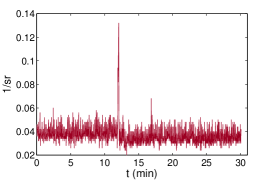
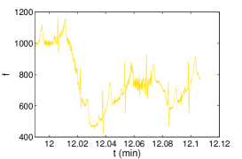
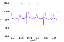
Figure 4: The left graph shows the inverse local sparsity values for each segment in the signal partition of record 117. The middle graph is the piece of signal where the peak of $1/\mathrm{sr}$ takes place. The right graph is a piece of signal of the same length but at different time interval.

5 Conclusions

A method for dimensionality reduction of ECG signals has been proposed. The approach was designed within the framework of sparse representation. A number of wavelet based dictionaries have been introduced to undertake the signal model via the OOMP greedy strategy. The resulting representation was shown to require significantly less elementary component than those needed when using a wavelet basis. The method was proven to be useful for ECG compression at low level distortion. The compression results largely surpass benchmarks within the state of the art for the MIT-BIH Arrhythmia database.

The MATLAB software for constructing the dictionaries and reproducing the results in the paper has been made available on a dedicated website. Although the numerical construction of the signal model is computationally intensive it can be effectively realized, even in the MATLAB environment, where it typically takes 30 s to compress a 30 min record and 1 s to recover the signal from the compressed file. Moreover, since the approximation is carried out independently in every segment of the signal partition, there is room for straightforward parallelization using multiprocessors. The sensitivity of local sparsity to nonstationary noise or significant distortion of patterns leads to conclude that the model might be useful to support the development of techniques for analysis of ECG records.

References

- [1] S. Banerjee, M. Mitra, “Application of Cross Wavelet Transform for ECG pattern analysis and classification”, IEEE Transactions on Instrumentation and Measurement, 63 326–333 (2014).
- [2] R.G. Afkhami, G. Azarnia, M.A. Tinati, “Cardiac arrhythmia classification using statistical and mixture modeling features of ECG signals, Pattern Recognition Letters, 70, 45– 51 (2016).
- [3] S. Shadmand, B. Mashoufi, “A new personalized ECG signal classification algorithm using block-based neural network and particle swarm optimization, Biomedical Signal Processing and Control, 25, 12–23 (2016).
- [4] E.J.D. Luz, W.R. Schwartz, G. Camara-Chavez, D. Menotti, ECG-based heartbeat classification for arrhythmia detection: a survey, Computer Methods and Programs in Biomedicine, 127 144–164 (2016).
- [5] D. P. Tobón V., T. H. Falk, M. Maier, “MS-QI: A Modulation Spectrum-Based ECG Quality Index for Telehealth Applications”, IEEE Transactions on Biomedical Engineering, 63, 1613– 1622 (2016).
- [6] S. Gutta, Q. Cheng, “Joint feature extraction and classifier design for ECG-based biometric recognition”, Journal of Biomedical and Health Informatics, 20, 460–468 (2016).
- [7] H. Li, D. Yuan, Y. Wang, D. Cui, and L. Cao, “Arrhythmia Classification Based on Multi-Domain Feature Extraction for an ECG Recognition System”, Sensors, 16, doi:10.3390/s16101744 (2015).
- [8] M. Abdelazez, P. X. Quesnel, A. D. C. Chan, H. Yang, “Signal Quality Analysis of Ambulatory Electrocardiograms to Gate False Myocardial Ischemia Alarms”, IEEE Transactions on Biomedical Engineering, 64, 1318 – 1325 (2018).
- [9] S. K. Berkaya, A. K. Uysal, E. S. Gunal, S. Ergin., S. Gunal, M. B. Gulmezoglu, “A survey on ECG analysis”, Biomedical Signal Processing and Control, 43, 216 – 235 (2018).
- [10] H. Mamaghanian, N. Khaled, D. Atienza and P. Vandergheynst, “Compressed Sensing for Real-Time Energy-Efficient ECG Compression on Wireless Body Sensor Nodes”, IEEE Transactions on Biomedical Engineering, 58, 2456 – 2466 (2011).
- [11] Z. Zhang, T-P Jung, S. Makeig and B. D. Rao, “Compressed Sensing for Energy-Efficient Wireless Telemonitoring of Noninvasive Fetal ECG via Block Sparse Bayesian Learning”, IEEE Transactions on Biomedical Engineering, 60, 300–309 (2013).
- [12] L. F. Polanía, R. E. Carrillo, Manuel Blanco-Velasco and K. E. Barner, “Exploiting Prior Knowledge in Compressed Sensing Wireless ECG Systems”, IEEE Journal of Biomedical and Health Informatics, 19, 508–519 (2015).
- [13] G. Da Poian, R. Bernardini, R. Rinaldo, ‘RSeparation and Analysis of Fetal-ECG Signals From Compressed Sensed Abdominal ECG Recordings”, IEEE Transactions on Biomedical Engineering, 63, 1269 – 1279 (2016).
- [14] L. F. Polanía and R. I. Plaza, “Compressed Sensing ECG using Restricted Boltzmann Machines”, Biomedical Signal Processing and Control, 45, 237–45 (2018).
- [15] R. Baraniuk, “Compressive sensing”, IEEE Signal Processing Magazine, 24, 118–121, (2007).
- [16] E. Candès and M. Wakin, “An introduction to compressive sampling”, IEEE Signal Processing Magazine, 25, 21 – 30 (2008).
- [17] M. S Manikandan and S. Dandapat, “Wavelet-based electrocardiogram signal compression methods and their performances: A prospective review”, Biomedical Signal Processing and Control, 14, 73–107 (2014).
- [18] http://www.nonlinear-approx.info/examples/node011.html (Last access May 2018).
- [19] L. Rebollo-Neira and D. Lowe, “Optimized orthogonal matching pursuit approach”, IEEE Signal Process. Letters, 9, 137–140 (2002).
- [20] L. Rebollo-Neira, “Cooperative greedy pursuit strategies for sparse signal representation by partitioning”, Signal Processing, 125, 365–375 (2016).
- [21] M. Andrle and L. Rebollo-Neira, “Cardinal B-spline dictionaries on a compact interval”, Appl. Comput. Harmon. Anal. , 18, 336-346 (2005).
- [22] M. Andrle and L. Rebollo-Neira, “From cardinal spline wavelet bases to highly coherent dictionaries”, Journal of Physics A 41 (2008) 172001.
- [23] L. Rebollo-Neira and Z. Xu, “Adaptive non-uniform B-spline dictionaries on a compact interval”, Signal Processing, 90, 2308–2313 (2010).
- [24] L. L. Schumaker, Spline Functions: Basic Theory, Wiley, New-York, 1981.
- [25] C. Chui and J. Wang, “On compactly supported spline wavelets and a duality principle”, Trans. Amer. Math. Soc., 330, 903–915 (1992).
- [26] A. Cohen, I. Daubechies, and J.C. Feauveau, “Biorthogonal bases of compactly supported wavelets”, Comm. Pure and Appl. Math., 45, 485–560 (1992).
- [27] I. Daubechies, “Orthonormal bases of compactly supported wavelets”, Commun. Pure Appl. Math., 41, 909–996 (1988).
- [28] I. Daubechies, “Orthonormal bases of compactly supported wavelets II, variations on a theme”, SIAM J. Math. Anal., 24, 499–519 (1993).
- [29] D. Černá, V. Finěk, and K. Najzar, “On the exact values of coefficients of coiflets”, Cent. European J. Math. 6, 159–169 (2008).
- [30] D. Chen, “Spline wavelets of small support”, SIAM J. Math. Anal., 26, 500–517 (1995).
- [31] B. Han and Z. Shen, “Wavelets with short support”, SIAM J. Math. Anal., 38, 530–556 (2006).
- [32] L. Rebollo-Neira and I. Sanches, , “Simple scheme for compressing sparse representation of melodic music”, Electronics Letters (2017) DOI:10.1049/el.2017.3908
- [33] L. Rebollo-Neira, “A competitive scheme for storing sparse representation of X-Ray medical images” (2018) PLOS ONE. https://doi.org/10.1371/journal.pone.0201455.
- [34] L. A. Wasser, “Hierarchical Data Formats - What is HDF5?”, https://www.neonscience.org/about-hdf5 (2015)
- [35] https://physionet.org/physiobank/database/mitdb/ (Last access May 2018).
- [36] K. Skretting, http://www.ux.uis.no/karlsk/proj99 (Last access May 2018).
- [37] L. Rebollo-Neira, “Effective high compression of ECG signals at low level distortion”, Scientific Reports 9, Article number: 4564 (2019).
- [38] J. Wang, M. She, S. Nahavandi, A. Kouzani, “Human Identification From ECG Signals Via Sparse Representation of Local Segments”, IEEE Signal Processing Letters, 20, 937 – 940 (2013).
- [39] S. Raj, K. C. Ray, “Sparse representation of ECG signals for automated recognition of cardiac arrhythmias”, Expert Systems with Applications, 105, 49–64 (2018).
- [40] S.J. Lee, J. Kim and M. Lee,“A Real-Time ECG Data Compression and Transmission Algorithm for an e-Health Device”, IEEE Transactions on Biomedical Engineering, 58, 2448–2455 (2011).
- [41] J.L. Ma, T.T. Zhang and M. C. Dong, “A Novel ECG Data Compression Method Using Adaptive Fourier Decomposition With Security Guarantee in e-Health Applications”, IEEE Journal of Biomedical and Health Informatics, 19, 986–994 (2015).
- [42] C. Tan, L. Zhang and H. Wu,“A Novel Blaschke Unwinding Adaptive Fourier Decomposition based Signal Compression Algorithm with Application on ECG Signals”, IEEE Journal of Biomedical and Health Informatics 10.1109/JBHI.2018.2817192, 22 March 2018.
- [43] A. Pandey, B. Singh, S Sain, and N. Sood, “A joint application of optimal threshold based discrete cosine transform and ASCII encoding for ECG data compression with its inherent encryption”, Australasian Physical and Engineering Sciences in Medicine, 39, 833–855 (2016).