G-Warm inflation: Intermediate model

Abstract

A warm-intermediate inflationary universe model is studied in the presence of the Galileon coupling $G(\phi,X)=g(\phi)X$. General conditions required for successful inflation are deduced and discussed from the background and cosmological perturbations under slow-roll approximation. In our analyze we assume that the dynamics of our model evolves accordingly two separate regimes, namely $3g\dot{\phi}H\gg 1+R$, i.e., when the Galileon term dominates over the standard kinetic term and the dissipative ratio, and secondly in the regime where both $3g\dot{\phi}H$ and $R$ become of the same order than unity. For these regimes and assuming that the coupling parameter $g=g_{0}=$ constant, we consider two different dissipative coefficients $\Gamma$; one constant and the other being a function of the inflaton field. Furthermore, we find the allowed range in the space of parameters for our G-warm model by considering the latest data of Planck and also the BICEP2/Keck-Array data from the $r=r(n_{s})$ plane, in combination with the conditions in which the Galileon term dominates and the thermal fluctuations of the inflaton field predominate over the quantum ones.

I Introduction

The paradigm of cosmic inflation during the very early universe is arguably the most successful scenario for explaining several puzzling features of the Hot Big-Bang theory (HBB), as the horizon, flatness, monopole problems, among others R1 ; R102 ; R106 ; R103 ; R104 ; R105 . One of the most interesting features of inflation is that it can create primordial perturbations R2 ; R202 ; R203 ; R204 ; R205 . These primordial perturbations seed the temperature anisotropies that are observed in the cosmic microwave background (CMB) Aghanim:2018eyx ; Ade:2015xua ; Ade:2013zuv , as well as the observed large-scale structure (LSS) of the universe. Indeed, the simplest inflation model, which consists in a single field with a canonical kinetic term and an enough flat potential minimally coupled to gravity, give predictions that are in agreement with current observational data Akrami:2018odb ; Array:2015xqh ; Ade:2015lrj ; Planck:2013jfk .

The standard picture of inflation requires two separate phases as follows: first, during the slow-roll phase, the universe undergoes an accelerating expansion during which its energy density is dominated by the potential term of the inflaton scalar field. Subsequently, during the reheating phase Kofman:1997yn ; Kofman:1994rk , the inflaton oscillates around the minimum of its potential by dissipating its energy to a radiation bath. Consequently, the universe enters the radiation era of the standard HBB model. For comprehensive reviews on several aspects of reheating phase, see Refs.Amin:2014eta ; Allahverdi:2010xz . An alternative scenario, called warm inflation warm1 ; warm2 , offers the possibility that the inflaton field dissipates its energy into a radiation bath during the slow-phase, triggered by a friction term added to the background equations. In this sense, warm inflation is opposed to the conventional cold inflation avoiding the reheating stage. In the framework of warm inflation the Universe smoothly enters the radiation era, wherewith a reheating phase is no longer required after the end of inflationary epoch. An useful way to parametrize the effectiveness of warm inflation is trough the ratio $R\equiv\Gamma/3H$, where $\Gamma$ denotes the dissipative coefficient (or else decay ratio) and $H$ the Hubble rate. The weak dissipative regime for warm inflation corresponds to the condition $R\ll 1$, while $R\gg 1$ characterizes the strong dissipative regime of warm inflation. It is worth to mention that the parameter $\Gamma$, may be computed from first principles in quantum field theory, taking into account that the microscopic physics resulting from the interactions between the inflaton and other degrees of freedom BasteroGil:2012cm ; Bartrum:2013fia ; Zhang:2009ge ; 26 ; 28 ; PRD . In general terms, the decay rate for the inflaton field may depend on the scalar field itself or the temperature of the thermal bath, or both quantities, or even it can be a constant. Furthermore, thermal fluctuations may play a fundamental role in warm inflation scenario regarding the production of primordial fluctuations 6252602 ; 1126 ; 6252603 . In this sense, the density perturbations arise from thermal fluctuations of the inflaton which dominate over the quantum fluctuations. So that, an essential condition for warm inflation to occur is the presence of a radiation component whose temperature is such that $T>H$, since the thermal and quantum fluctuations are proportional to $T$ and $H$, respectively warm1 ; warm2 ; 6252602 ; 1126 ; 6252603 ; 6252604 ; 62526 ; Moss:2008yb ; Ramos:2013nsa . For a comprehensive review and a representative list of recent references of warm inflation can be seen in Refs. Berera:2008ar ; Ramos:2016coz and Das:2018rpg ; Motaharfar:2018zyb ; Bastero-Gil:2018uep ; Li:2018wno ; Herrera:2018cgi , respectively.

In relation to exact solutions for canonical single field inflation in the framework of General Relativity (GR), one of the most appealing comes from a constant potential for the inflaton field, which yields to de Sitter expansion R1 . On the other hand, a power-law dependence of the scale factor in cosmic time, i.e. $a(t)\propto t^{p}$, where $p>1$, is obtained when an exponential potential for the inflaton field is introduced Lucchin:1984yf . Yet another exact solution corresponds to intermediate inflation model, for which the scale factor evolves with cosmic time as follows Barrow:1990vx

$$a(t)=\exp\left[A\,t^{f}\right],$$ (1)

where $A$ and $f$ are constant parameters, satisfying the conditions $A>0$ and $0<f<1$. This expansion law becomes slower than de Sitter inflation, but faster than power-law inflation instead. Although intermediate inflationary model was introduced as an exact solution, this expansion gives a particular scalar field potential of the type $V(\phi)\propto\phi^{-4(f^{-1}-1)}$ Barrow:1993zq . However, the predictions of this model, regarding primordial perturbations, may be studied under the slow-roll approximation Barrow:1993zq ; Barrow:2006dh . In this form, at lowest order in the slow-roll approximation, this model predicts that the scalar spectral index becomes $n_{s}=1$ when $f=2/3$, corresponding to the Harrison-Zel’dovich spectrum, which is ruled out by current observations. In addition, the predictions of this model on the $n_{s}-r$ plane lie outside the joint 95$\%$ CL contour for any value of $f$ Barrow:2006dh ; Ade:2015lrj ; Planck:2013jfk . It is worth to mention that, the intermediate inflation model can be rescued in the stage of warm inflation thanks to the modified dynamics Kamali:2016frd ; Herrera:2016sov ; Herrera:2015aja ; Herrera:2014nta ; Herrera:2014mca ; Herrera:2013rra .

Going further the standard canonical inflaton scenario, there are other single-field models constructed in the framework of Hordndeski Horndeski:1974wa , or generalized Galileon theories Nicolis:2008in ; Deffayet:2011gz ; Kobayashi:2011nu ; Charmousis:2011bf , which is the most general four-dimensional scalar-tensor theories in curved space-time, free of ghosts and instabilities, with second-order equations of motion. Of particular interest is potential-driven inflation in the presence of a cubic Galileon coupling given by $X\Box\phi$ (where $X=-g^{\mu\nu}\partial_{\mu}\phi\partial_{\nu}\phi/2$)DeFelice:2011hq . Here, the Galileon term may suppress the tensor-to-scalar ratio and eventually turn viable some inflationary potentials already discarded by current data in the canonical scenario, see e.g., Tsujikawa:2014rta ; Ohashi:2012wf . Recently, the efforts have been focused in building the so-called generalized G-inflation models Kobayashi:2011nu , consisting in a general term $G(\phi,X)\Box\phi$, which is included to the action for scalar field in addition to the standard kinetic term (for recent references, see Herrera:2018mvo ; Ramirez:2018dxe ; Maity:2018ipt ; Hirano:2016gmv ; Unnikrishnan:2013rka ). It is worth to mention that the construction of such a model deserves a careful analysis in order to prevent the appearance of instabilities and having successful inflation Kobayashi:2011nu ; Ohashi:2012wf ; Kamada:2010qe ; Kobayashi:2010cm ; Burrage:2010cu , as well as a subsequent stage of reheating BazrafshanMoghaddam:2016tdk . For instance, the authors in Ohashi:2012wf studied chaotic and natural inflation in a Galileon scenario $G(\phi,X)=f(\phi)X$, for two expressions of the coupling function $f(\phi)$, $f=c/M^{3}$ and $f\propto\phi$ discussed in DeFelice:2011hq ; Kamada:2010qe . Interestingly, they found that if the Galileon self-interaction dominates over the standard kinetic term after inflation, the oscillatory stage of reheating may not take place unless the mass scales characterizing the several potentials satisfy stringent constraints in comparison to the canonical case. Alternatively, if dissipative effects during inflation are taken into account, is possible to study the dynamics of warm inflation scenario in the presence of a Galileon term. This possibility was addressed first in Ref.Herrera:2017qux , and subsequently following the same line for the thermal fluctuations in Ref.Motaharfar:2017dxh . Particularly, in Herrera:2017qux , it was studied the Galilean term $G(\phi,X)=g(\phi)X$, when the coupling constant $g$ and the decay rate $\Gamma$ are constant. Here, considering the exponential potential, it was found the possibility of distinguish pure warm inflation or pure generalized G-inflation from the background and of the thermal fluctuations. In addition, the modified dynamics may yield a tensor-to-scalar ratio much smaller than those obtained in a standard G-inflation scenario, see e.g., Herrera:2017qux ; Unnikrishnan:2013rka .

Regarding the viability of the intermediate inflation in G-inflation scenarios for the cold models, in Refs.Teimoori:2017jzo and Herrera:2018ker , the authors studied the inflationary dynamics for such an expansion law for a Galileon term $G(\phi,X)\propto X^{n}$ and $G(\phi,X)\propto\phi^{\nu}X^{n}$, respectively. For both Galileon couplings, it was found the importance of the power $n$ in order to make compatible the intermediate inflation model with current observations. In particular, the authors in Herrera:2018ker found that for $n>38$ the tensor-to-scalar ratio becomes compatible with the bound $r_{0\textup{.}05}<0\textup{.}07$ (95 $\%$ CL), set by the BICEP2/Keck-Array collaboration Array:2015xqh . So that, intermediate inflation in the framework of cold model is still rule out for the Galileon term $G(\phi,X)\propto X$ ($n=1$) .

In this form, the main goal of the present paper is to explore the viability of the intermediate model in the context of the warm inflation scenario in which the Galileon term is given by $g(\phi)X$. In doing so, we consider a constant coupling function $g_{0}$ and in order to parametrize the dissipative effects, we consider two several expressions for the decay rate: $\Gamma=\Gamma_{0}$ and $\Gamma(\phi)\propto V(\phi)$, respectively. Thus, for each expression of the parameter $\Gamma$, we will be studied the background as well perturbative dynamics for two separate regimes. Firstly, we will consider the regime in which the quantity $3g_{0}\dot{\phi}H\gg 1+R$, i.e., when the Galileon term dominates over the standard kinetic term and the dissipative ratio. Secondly we will analyze the regime where both quantities $3g\dot{\phi}$ and $R$ become of the same order than unity. For all the cases, we will obtain the allowed range in the space of parameters. In this sense, we will consider the condition for warm inflation $T>H$, the conditions for the regimes $3g_{0}\dot{\phi}H\gg 1+R$ and $R\sim 3g_{0}\dot{\phi}H\sim 1$, respectively, together with the constraints on the $n_{s}-r$ plane by latest observational data.

The paper is organized as follows: The next section presents a general set up of warm inflation scenario in the presence of a Galileon term $G(\phi,X)=g(\phi)X$ at background level as well as perturbation level, where expressions for the most relevant cosmological observables as the power spectrum of scalar perturbations, scalar spectral index, and the tensor-to-scalar ratio will be obtained. Subsequently, in Section III, the background and perturbative dynamics for our concrete intermediate inflation will be study in the dominated Galileon regime for $\Gamma=\Gamma_{0}$ and $\Gamma(\phi)\propto V(\phi)$, respectively. Section IV is devoted to study the dynamics of our model evolving according to the general regime $R\sim 3g_{0}\dot{\phi}H\sim 1$, also for the cases in which $\Gamma=\Gamma_{0}$ and $\Gamma(\phi)\propto V(\phi)$, respectively. Finally, Section V, summarizes our results and presents our conclusions. We use units in which $c=\hbar=M_{p}$=8$\pi$=1.

II G-Warm inflation: Basic equations.

In this section we give a brief review on the scenario of G-warm inflation. We start by writing down the 4-dimensional action for this model

$$S=\int\sqrt{-g_{4}}\left({R\over 2}+K(\phi,X)-G(\phi,X)\,\Box\phi\right)d^{4}x+S_{\gamma}+S_{int}\,.$$ (2)

Here the quantity $g_{4}$ denotes the determinant of the space-time metric $g_{\mu\nu}$, $R$ corresponds to the Ricci scalar, $\phi$ denotes the scalar field and $X=-g^{\mu\nu}\partial_{\mu}\phi\partial_{\nu}\phi/2$. Besides, the quantities $K$ and $G$ are arbitrary functions of $X$ and the scalar field $\phi$. Additionally, we consider that the action for the perfect fluid describing radiation is defined by $S_{\gamma}$ and the interaction action is given by $S_{int}$. In this context, $S_{int}$ corresponds to the interaction between the scalar field and other degrees of freedom Herrera:2017qux ; nw1 ; nw2 .

By assuming a spatially flat Friedmann-Robertson-Walker (FRW) metric, the Friedmann equation can be written as

$$3H^{2}=\,\rho=\,[\rho_{\phi}+\rho_{\gamma}],$$ (3)

where the total energy density $\rho$ is given by $\rho=\rho_{\phi}+\rho_{\gamma}$, whit $\rho_{\phi}$ corresponding to the energy density of the scalar field $\phi$ and $\rho_{\gamma}$ denotes the energy density of the radiation field, respectively.

Following Refs.DeFelice:2011hq ; Kobayashi:2010cm , we can identify that the energy density and pressure related to the scalar field from the action (2) are given by

$$\rho_{\phi}=2K_{X}X-K+3G_{X}H\dot{\phi}^{3}-2G_{\phi}X\,,$$ (4)

and

$$p_{\phi}=K-2(G_{\phi}+G_{X}\ddot{\phi})X\,,$$ (5)

respectively. In the following, we will consider a homogeneous scalar field, i.e. $\phi=\phi(t)$ and the subscript $K_{X}$ corresponds to $K_{X}=\partial K/\partial X$, $G_{\phi}$ to $G_{\phi}=\partial G/\partial\phi$, $K_{XX}=\partial^{2}K/\partial X^{2}$, and so on.

As it was already mentioned, in the scenario of warm inflation, the universe is filled with a self-interacting scalar field and a radiation fluid. In this context, the dynamical equations for the densities $\rho_{\phi}$ and $\rho_{\gamma}$ can be written as warm1 ; warm2

$$\dot{\rho_{\phi}}+3\,H\,(\rho_{\phi}+p_{\phi})=-\Gamma\;\;\dot{\phi}^{2},$$ (6)

and

$$\dot{\rho}_{\gamma}+4H\rho_{\gamma}=\Gamma\dot{\phi}^{2}.$$ (7)

Here, we emphasize that the coefficient $\Gamma>0$ corresponds to the dissipation coefficient and its dependence can be considered to be a function of the temperature of the thermal bath $T$, in which $\Gamma(T)$, or the scalar field $\Gamma(\phi)$, or both $\Gamma(T,\phi)$ or simply a constantwarm1 ; warm2 . Recall that, the role of the coefficient $\Gamma$ is to account of the decay of the scalar field into radiation during the inflationary stage.

From Eqs.(4) and (5) we can rewrite Eq.(6) as

$$3\dot{H}G_{X}\,\dot{\phi}^{2}+\ddot{\phi}\left[3HG_{XX}\,\dot{\phi}^{3}-\dot{\phi}^{2}(G_{\phi X}-K_{XX})+6HG_{X}\,\dot{\phi}-2G_{\phi}+K_{X}\right]$$

$$+3HG_{\phi X}\,\dot{\phi}^{3}+\dot{\phi}^{2}(9H^{2}G_{X}-G_{\phi\phi}+K_{\phi X})-K_{\phi}-3H\dot{\phi}(2G_{\phi}-K_{X})=-\Gamma\dot{\phi}\,.$$ (8)

In order to study our model in the G-warm inflation scenario, we will consider the specific case in which the functions $K(\phi,X)$ and $G(\phi,X)$ are given by

$$K(\phi,X)=X-V(\phi),\qquad\text{and}\qquad G(\phi,X)=g(\phi)\,X\,,$$ (9)

where, the quantity $V(\phi)$ denotes the effective potential and the coupling parameter $g$ is a function that only depends on the scalar field i.e., $g=g(\phi)$.

In the context of warm inflation, the energy density related to the inflaton field $\rho_{\phi}$ dominates over the energy density of the radiation field $\rho_{\gamma}$ during the inflationary epoch, wherewith $\rho_{\phi}\gg\rho_{\gamma}$ warm1 ; warm2 ; 6252602 ; 1126 ; 6252603 ; 6252604 ; 62526 . Also, considering the slow roll approximation in which the effective potential $V(\phi)$ dominates over the functions $X$, $|G_{X}H\dot{\phi}^{3}|$ and $|G_{\phi}X|$, see e.g. Kobayashi:2010cm , then the Friedmann equation given, by Eq.(3), is reduced to

$$3H^{2}\approx\rho_{\phi}\approx V(\phi).$$ (10)

By assuming the slow-roll approximation, we can also introduce the set of slow-roll parameters for G-inflation, defined as Kobayashi:2010cm

$$\varepsilon_{1}={(-\dot{H})\over H^{2}},\quad\epsilon_{2}={(-\ddot{\phi})\over H\dot{\phi}},\quad\epsilon_{3}={g_{\phi}\dot{\phi}\over gH},\quad\text{and}\quad\epsilon_{4}={g_{\phi\phi}X^{2}\over V_{\phi}}\,.$$ (11)

In this sense, after replacing the functions $K$ and $G$ given by Eq.(9), together with the set of slow roll parameters given by Eq.(11), we rewrite the equation of motion for $\phi$ given by (8) as follows

$$3H\dot{\phi}(1-\epsilon_{2}/3+R)+3gH^{2}\dot{\phi}^{2}[3-\varepsilon_{1}-2\epsilon_{2}+2\epsilon_{2}\epsilon_{3}/3]=-V_{\phi}(1-2\epsilon_{4})\,.$$ (12)

Here, $R$ denotes the ratio between $\Gamma$ and the Hubble rate and it is defined as $R=\frac{\Gamma}{3H}$.

Thus, under the slow-roll approximation in which the parameters $|\varepsilon_{1}|,|\epsilon_{2}|,|\epsilon_{3}|,|\epsilon_{4}|\ll 1$, we obtain that the slow-roll equation of motion for the inflaton field (12) is reduced to Herrera:2017qux

$$3H\dot{\phi}(1+R+\mathcal{A})\simeq-V_{\phi}\,,$$ (13)

where the function $\mathcal{A}$ is defined as $\mathcal{A}=3\,g(\phi)H\dot{\phi}$. From the Friedmann equation (10), we find that the Eq.(13) can be rewritten as

$$\dot{\phi}^{2}(1+R+\mathcal{A})\simeq 2(-\dot{H})\,.$$ (14)

For the radiation field, we assume that during the stage of warm inflation, the radiation production is quasi-stable, implying that $\dot{\rho}_{\gamma}\ll 4H\rho_{\gamma}$ and $\dot{\rho}_{\gamma}\ll\Gamma\dot{\phi}^{2}$warm1 ; warm2 ; 6252602 ; 1126 ; 6252603 ; 6252604 ; 62526 . In this form, during inflation, Eq.(7) becomes

$$\rho_{\gamma}\simeq\frac{\Gamma\dot{\phi}^{2}}{4H}.$$ (15)

We note that the energy density $\rho_{\gamma}$ and the temperature of the thermal bath $T$ are related through $\rho_{\gamma}=C_{\gamma}\,T^{4}$, where $C_{\gamma}=\pi^{2}\,g_{\ast}/30$ and $g_{\ast}$ corresponds to the number of relativistic degrees of freedom. Thus, the temperature of the thermal bath, considering Eq.(15) can be expressed as

$$T\simeq\left[\frac{\Gamma\dot{\phi}^{2}}{4C_{\gamma}H}\right]^{1/4}.$$ (16)

In G-warm inflation, one may distinguish several regimes, see ref.Herrera:2017qux . From the slow-roll equation given by Eq.(13), the regimes $R+3gH\dot{\phi}\ll 1$ and $1+3gH\dot{\phi}\ll R$ are the standard weak and strong dissipative regimes in the scenario of warm inflation for a canonical scalar field, respectively. Now, in G-warm inflation we can also have the regime $1+R\ll|gH\dot{\phi}|$,where the Galileon coupling dominates during the inflationary epoch and therefore the dynamics of standard or pure warm inflation is modified. Also, another two interesting regimes were studied in ref.Herrera:2017qux . Here, the standard weak and strong dissipative regimes are mixed with the Galileon effect, and these correspond to $R\ll 1+3gH\dot{\phi}$ and $1\ll R+3gH\dot{\phi}$, respectively.

At background level, another important quantity is the number of $e$-folds $N$ between two different values of cosmological times $t_{1}$ and $t_{2}$, defined as $N=\int_{t_{1}}^{t_{2}}\,H\,dt$. In particular for intermediate inflation, $N$ is given by

$$N=\int_{t_{1}}^{t_{2}}\,H\,dt=A\,\left(t_{2}^{f}-t_{1}^{f}\right).$$ (17)

In this sense, we noted that the Hubble rate assuming the intermediate expansion can be expressed in terms of the $e$-folds $N$ as follows

$$H(N)=Af\,\left[{Af\over 1+f(N-1)}\right]^{1-f\over f},$$ (18)

and $\dot{H}=\dot{H}(N)$ as

$$\quad-\dot{H}(N)=Af(1-f)\,\left[{Af\over 1+f(N-1)}\right]^{2-f\over f}.$$ (19)

Here, we have considered that the inflationary scenario begins at the earliest possible stage in which $\varepsilon_{1}(t=t_{1})=-\dot{H}/H^{2}=1$Barrow:1990vx ; Barrow:1993zq . We also mentioned that during intermediate expansion, the slow-roll parameter $\varepsilon_{1}$ in terms of the number of $e$-folds $N$ becomes

$$\varepsilon_{1}=-\frac{\dot{H}}{H^{2}}=\frac{1-f}{1+f(N-1)}.$$ (20)

This suggests that the inflationary epoch begins at the earliest possible stage when the number of $e$-folding is equal to $N=0$. or equivalently $\varepsilon_{1}\equiv 1$. Note that when $N\gg 1$, the slow-roll parameter $\varepsilon_{1}\rightarrow 0$, implying that inflation never ends. However, in the context of warm inflation the universe smoothly enters to the radiation era, since the radiation field dominates over the energy density of the inflaton according as the universe expands warm1 ; warm2 , see also Ref.sh as other mechanisms for address the end of the accelerated expansion and the reheating of the universe or this expansion law.

On the other hand, the cosmological perturbation theory in the model of G-warm inflation was developed in Ref.Herrera:2017qux . In this context, the source of the density fluctuations corresponds to thermal fluctuations of the inflaton field during inflation. Thus, according to the evolution of warm inflation, the fluctuations of the inflaton field $\delta\phi$ are dominantly thermal rather than quantum, see refs. warm1 ; warm2 ; 6252602 ; 1126 ; 6252603 ; 6252604 ; 62526 ; Moss:2008yb ; Ramos:2013nsa . In order to determine the amplitude of the fluctuations is necessary to consider the Langevin equation that includes a thermal stochastic noise term in the KG equation. In this way, the fluctuations of the scalar field $\delta\phi$ in G-warm model for the case in which the dissipation coefficient $\Gamma=\Gamma(\phi)$, can be written as $\delta\phi^{2}\simeq\sqrt{3H^{2}+H\Gamma+18gH^{3}\dot{\phi}}\,\,\,T/2\pi^{2}$, see ref.Herrera:2017qux . Here, we noted that in the limit $g\rightarrow 0$, the fluctuations of the scalar field $\delta\phi$ reduces to the fluctuations found in the case of pure warm inflation warm1 ; warm2 ; 6252602 ; 1126 ; 6252603 ; 6252604 ; 62526 ; Moss:2008yb ; Ramos:2013nsa . In this form, following Herrera:2017qux , the power spectrum of the scalar perturbation defined by ${\mathcal{P}_{\mathcal{R}}}=(H/\dot{\phi})^{2}\delta\phi^{2}$, can be written as

$${\mathcal{P}_{\mathcal{R}}}={1\over 2\pi^{2}}\left({H\over\dot{\phi}}\right)^{2}\left[{\Gamma\,X\over 2C_{\gamma}\,H}\right]^{1/4}\sqrt{3H^{2}(1+6gH\dot{\phi})+\Gamma\,H}.$$ (21)

By using the fact that the rate $R=\Gamma/3H$ and the function $\mathcal{A}=3\,g\,H\dot{\phi}$, then the scalar perturbation ${\mathcal{P}_{\mathcal{R}}}$ can be rewritten as

$${\mathcal{P}_{\mathcal{R}}}={\sqrt{3}\over 2\pi^{2}}\left({3\over 4C_{\gamma}}\right)^{1\over 4}\left(H^{3}R^{1\over 4}\right)\dot{\phi}^{-{3\over 2}}\sqrt{1+R+2\mathcal{A}}\,.$$ (22)

As the scalar spectral index $n_{s}$ is given by $n_{s}-1=\frac{d\ln\,{\cal{P}_{R}}}{d\ln k}$, we find that the spectral index $n_{s}$ results

$$n_{s}\simeq 1-\frac{\epsilon_{1}}{2}\left[\frac{7}{2}+\frac{1+12gH\dot{\phi}}{(1+R+6gH\dot{\phi})}\right]+3\epsilon_{2}\left[\frac{1}{4}-\frac{gH\dot{\phi}}{(1+R+6gH\dot{\phi})}\right]+\epsilon_{3}\left[\frac{3gH\dot{\phi}}{(1+R+6gH\dot{\phi})}\right]$$

$$+\frac{\epsilon_{5}}{2}\left[\frac{1}{2}+\frac{R}{(1+R+6gH\dot{\phi})}\right],$$ (23)

where the quantity $\epsilon_{5}$ is defined as $\epsilon_{5}=\left(\frac{\dot{\phi}}{H}\right)\,\left(\frac{\Gamma_{\phi}}{\Gamma}\right).$ Here, we have used Eq.(22).

It is well known that tensor perturbations during inflation would generate gravitational waves (GWs). In the case of G-inflation, the amplitude of the tensor perturbations is the same as in the case of standard general relativity (GR)DeFelice:2011hq ; Kobayashi:2010cm . So that, the the amplitude of the tensor perturbations is given by

$${\cal{P_{G}}}={2H^{2}\over\pi^{2}}.$$ (24)

Here, we have considered the slow-roll approximation given by Eq.(10).

Another important cosmological observable is the tensor-to-scalar ratio $r={\cal P_{G}}/\cal{P_{R}}$. Thus, from Eqs.(22) and (24) the tensor- scalar ratio can be written as

$$r=4\,X\,\left(\frac{2C_{\gamma}\,H}{\Gamma\,X}\right)^{1/4}\,[3H^{2}(1+6gH\dot{\phi})+H\Gamma]^{-1/2}\;.$$ (25)

In the following, we will study the intermediate expansion in the framework of G-warm inflation, for the simplest case in which the Galileon coupling function $g=g_{0}=$ constantDeFelice:2011hq ; Kobayashi:2010cm . Also, in this framework we will consider two different dissipative coefficients $\Gamma$. As well, we will restrict ourselves to the domination of the Galileon effect on standard warm inflation, i.e., $3gH\dot{\phi}={\cal{A}}\gg 1+R$ and we will also studied the regime where all terms of Eq.(13) are the same order i.e., $1\sim R\sim\cal{A}$, namely the general or full solution.

III Domination of the Galileon regime ${\mathcal{A}}\gg 1+R$.

In this section we utilize the formalism of above to G-warm inflation in the context of intermediate expansion, assuming that our G-warm model evolves according to the domination of the Galileon regime, in which the function ${\mathcal{A}}\gg 1+R$.

By assuming the limit ${\mathcal{A}}\gg 1+R$, we note that the background equations do not depend on the dissipation coefficient $\Gamma$. In this way, we find that the speed of scalar field $\dot{\phi}$ given by Eq.(13) results in

$$\dot{\phi}\simeq\left[{2(-\dot{H})\over 3\,g_{0}H}\right]^{1/3}.$$ (26)

As we mentioned above, we observed that $\dot{\phi}$ does not depend of the coefficient $\Gamma$. Now, from the intermediate scale factor given by Eq.(1), we obtain that the solution for the scalar field in terms of the cosmological time becomes

$$\phi(t)=\left[{9(1-f)\over 4\,g_{0}}\right]^{1/3}t^{2/3}+C_{0},$$ (27)

where $C_{0}$ denotes an integration constant, that without loss of generality it can be assumed $C_{0}=0$. From this solution, we find that the Hubble rate has the following dependence on the inflaton field

$$H(\phi)=A\,f\,\left[\frac{3}{2}\left({1-f\over g_{0}}\right)^{1\over 2}\right]^{(1-f)}\phi^{-{3(1-f)\over 2}}.$$ (28)

In this way, from Eqs.(10) and (28) we obtain that the effective potential in limit ${\mathcal{A}}\gg 1+R$ is given by

$$V(\phi)=V_{0}\,\phi^{-3(1-f)},\,\,\,\;\;\;\;\mbox{where}\;\,\,\,\,V_{0}=3A^{2}\,f^{2}\,\left[\frac{3}{2}\left({1-f\over g_{0}}\right)^{1\over 2}\right]^{2(1-f)}.$$ (29)

Note that this kind of scalar potential (power-law), which depends on the inflaton field in an inverse power-law way, does not have a minimum and it decays to zero for lager values of $\phi$, since $0<f<1$. We also note that this potential becomes independent of the dissipation coefficient $\Gamma$, as it was previously quoted.

On the other hand, the dimensionless slow-roll parameter $\varepsilon_{1}=-\dot{H}/H^{2}$ can be rewritten in terms of the inflaton field, considering the slow-roll approximation wherewith

$$\varepsilon_{1}=\left({\frac{1-f}{Af}}\right)\left[\frac{3}{2}\left({1-f\over g_{0}}\right)^{1\over 2}\right]^{f}\phi^{-{3\,f\over 2}}.$$

In this context, the condition of inflation to occur is given by $\varepsilon_{1}<$1, or analogously $\ddot{a}>0$. Therefore, the inflaton field during the inflationary epoch is such that $\phi>\left({\frac{1-f}{Af}}\right)^{{2\over 3\,f}}\left[\frac{3}{2}\left({1-f\over g_{0}}\right)^{1\over 2}\right]^{{2\over 3}}$. As we mentioned earlier, the inflationary phase begins at the earliest possible stage, i.e, $\varepsilon_{1}(\phi=\phi_{1})=1$. Then, the scalar field $\phi_{1}$, is given by $\phi_{1}=\left({\frac{1-f}{Af}}\right)^{{2\over 3\,f}}\left[\frac{3}{2}\left({1-f\over g_{0}}\right)^{1\over 2}\right]^{{2\over 3}}$. Also the number of $e$-folds $N$ defined between two different values of cosmological times $t_{1}$ and $t_{2}$ or equality between $\phi_{1}$ and $\phi_{2}$, by considering Eq.(27) can be written as

$$N=\int_{t_{1}}^{t_{2}}\,H\,dt=A\,\left(t_{2}^{f}-t_{1}^{f}\right)=\frac{2^{f}A}{3^{f}}\left({g_{0}\over 1-f}\right)^{f\over 2}\,\left(\phi_{2}^{3f/2}-\phi_{1}^{3f/2}\right).$$ (30)

From the number of e-folding $N$, it is possible to rewrite the function ${\mathcal{A}}=3g_{0}H\dot{\phi}$ in terms of $N$. Thus, from Eqs.(1), (26) and (30), we have that

$$\mathcal{A}(N)=2^{1\over 3}(3g_{0})^{2\over 3}(Af)(1-f)^{1\over 3}\left[{Af\over 1+f(N-1)}\right]^{4-3f\over 3f}.$$ (31)

Since the cosmological perturbations depend on the dissipation coefficient $\Gamma$, then in the following we will analyze our model in the limit ${\mathcal{A}}\gg 1+R$, for two specific cases of the dissipation coefficient $\Gamma$ studied in the literature, namely; $\Gamma(\phi)=\Gamma_{0}=$ constant warm1 ; warm2 and $\Gamma(\phi)\propto\,V(\phi)$delCampo:2007cy .

III.1 Case $\Gamma=\Gamma_{0}=$ constant.

Let us consider that our model of G-warm inflation evolves according to the regime ${\mathcal{A}}\gg 1+R$, when the dissipation coefficient $\Gamma$ has the following form, where $\Gamma=\Gamma_{0}=$ constantwarm1 ; warm2 . In this sense, from Eq.(22) we find that the power spectrum of the scalar perturbations ${\mathcal{P}_{\mathcal{R}}}$, can be rewritten as

$${\mathcal{P}}_{\mathcal{R}}={\Gamma_{0}^{1/4}P_{0}\over 3^{1/4}}\,H^{43\over 12}(-\dot{H})^{-{1\over 3}},\,\,\,\,\mbox{where}\,\,\,\,P_{0}=\frac{3^{19/12}\,g_{0}^{5/6}}{2^{4/3}\pi^{2}\,C_{\gamma}^{1/4}}.$$ (32)

Here, we have used Eq.(26). Now, by using Eq.(27), we can write the power spectrum of the scalar perturbation in terms of the inflaton field as

$${\mathcal{P}_{\mathcal{R}}}(\phi)=P_{I}\,\phi^{-\beta_{I}},\,\;\;\;\mbox{in which}\;\;\;\;P_{I}=P_{0}\left({\Gamma_{0}\over 3}\right)^{1\over 4}\left(Af\right)^{39\over 12}\left(1-f\right)^{-1\over 3}\left[\frac{3}{2}\left({1-f\over g_{0}}\right)^{1\over 2}\right]^{2\beta_{I}\over 3},$$ (33)

and $\beta_{I}$ is defined as $\beta_{I}=\left[{35-39f\over 8}\right]$. Note that for the particular case in which $f=35/39\simeq 0.90$, the power spectrum of the scalar perturbations becomes constant. From Eq.(30), we can rewrite the power spectrum of the scalar perturbation as a function of the number of $e$-folds $N$ as

$${\mathcal{P}_{\mathcal{R}}}(N)=p_{I}\,\left[{Af\over 1+f(N-1)}\right]^{2\beta_{I},\over 3f},$$ (34)

where the constant $p_{I}$ is defined as $p_{I}=P_{0}\left({\Gamma_{0}\over 3}\right)^{1\over 4}\left(Af\right)^{13\over 4}\left(1-f\right)^{-1\over 3}$.

As the scalar spectral index $n_{s}$ is defined as $n_{s}-1=\frac{d\ln\,{\mathcal{P}_{R}}}{d\ln k}$, we find that the index $n_{s}$ can be written in terms of the scalar field $\phi$ as

$$n_{s}=1-\left({35-39f\over 12Af}\right)\left[\frac{3}{2}\left({1-f\over g_{0}}\right)^{1\over 2}\right]^{f}\phi^{-{3\,f\over 2}}.$$ (35)

Also, we note that for the specific value of $f=35/39\simeq 0.90$, the scalar spectral index $n_{s}$ corresponds to a scale-invariant spectral index, for which $n_{s}=1$, called the Harrison-Zel’dovich spectrum of density perturbations. As we mentioned before, for intermediate inflation in the context of GR, the parameter $f=2/3$ corresponds to the value $n_{s}=1$. From Eq.(30), we also obtain the scalar spectral index $n_{s}$ as function of $N$, yielding

$$n_{s}=1-{35-39f\over 12[1+f(N-1)]}.$$ (36)

Note that from this equation we can express the parameter $f$ in terms of the spectral index and the number of $e$-folds as $f=\frac{12(n_{s}-1)+35}{3[13+4(1-n_{s})(N-1)]}$. In particular, for the number of e-folds $N=60$ and the scalar spectral index $n_{s}=0.967$, we find that the value of the parameter $f$ is given by $f\simeq 0.55$. Also, for $N=60$ and considering the current observational constraint for $n_{s}$ set by Planck, given by $n_{s}=0.964$, the parameter $f$ corresponds to $f\simeq 0.54$.

Furthermore, we can express the parameter $A$ of the intermediate expansion in terms of the quantities $g_{0}$, $\Gamma_{0}$, $N$, ${\mathcal{P}_{\mathcal{R}}}(N)$ and $f$ (or equivalently $n_{s}$) as

$$A=\left[\frac{3^{1/4}{\mathcal{P}_{\mathcal{R}}}}{f^{13/4}P_{0}\,\Gamma_{0}^{1/4}}(1-f)^{1/3}\left(\frac{1+f(N-1)}{f}\right)^{2\beta_{I}/3f}\right]^{\frac{12f}{39f+8\beta_{I}}}.$$ (37)

Here, we have considered Eq.(34).

From Eq.(25), the tensor-to-scalar ratio $r$ as a function of the scalar spectral index $n_{s}$ can be written as

$$r(n_{s})\simeq{2A^{2}f^{2}\over\pi^{2}\,p_{I}}\left[{35-39f\over 12Af(1-n_{s})}\right]^{11-15f\over 12f}.$$ (38)

We also mention that the ratio $R=\Gamma/3H$ can be expressed as a function of the number of $e$-folds by considering Eq.(30). In doing so, we have that the ratio $R=R(N)$ becomes

$$R(N)={\Gamma_{0}\over 3Af}\left[{1+f(N-1)\over Af}\right]^{1-f\over f}.$$ (39)

Similarly, from Eqs.(31), (36) and (39), we can obtain the effective function ${\mathcal{A}}-R$ in terms of the scalar spectral index $n_{s}$, resulting

$${\mathcal{A}}-R=[2(1-f)]^{1/3}(3g_{0})^{2/3}(Af)^{4/3f}\left[\frac{12(1-n_{s})}{35-39f}\right]^{\frac{4-3f}{3f}}-\frac{\Gamma_{0}}{3(Af)^{1/f}}\left[\frac{35-39f}{12(1-n_{s})}\right]^{\frac{1-f}{f}}.$$ (40)

Note that in order to achieve the domination of the Galileon coupling during the whole inflationary stage, we must take into account that ${\mathcal{A}}\gg 1+R$.

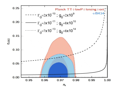
Figure 1: Plot of the tensor-to-scalar ratio $r$ against the scalar spectral index $n_{s}$(upper panel), and the the difference ${\mathcal{A}}-R$ as a functions of scalar spectral index $n_{s}$(lower panel), in the G-warm intermediate model when $\Gamma=\Gamma_{0}=$ const. For both panels we use three a different pair of values of ($\Gamma_{0},g_{0}$).

Also, the temperature of the thermal bath can be rewritten from Eq.(16) as

$$T=\left[\frac{\Gamma_{0}}{4C_{\gamma}}\right]^{1/4}\left[\frac{2}{3g_{0}}\right]^{1/6}H^{-5/12}(-\dot{H})^{1/6},$$ (41)

and from Eqs.(28),(35) and (41) the rate $T/H$ in terms of the scalar spectral index $n_{s}$ can be written as

$$\frac{T}{H}(n_{s})=\left[\frac{\Gamma_{0}}{4C_{\gamma}}\right]^{1/4}\left[\frac{2}{3g_{0}}\right]^{1/6}{(1-f)^{1/6}\over(Af)^{13/12f}}\left[{35-39f\over 12(1-n_{s})}\right]^{13-15f\over 12f}>1.$$ (42)

Here, we have considered that the essential condition for warm inflation to occur, is set by $T>H$ warm1 ; warm2 .

Fig.1 shows the tensor-to-scalar ratio $r$ versus the scalar spectral index $n_{s}$ (upper panel) and in the lower panel we show the necessary condition for domination of the Galileon term in which ${\mathcal{A}}-R\gg 1$ versus the scalar spectral index $n_{s}$, when $\Gamma=\Gamma_{0}=$ constant. For both plots, we have considered three different pairs of values $(\Gamma_{0},g_{0})$. In the upper panel are shown the two-dimensional marginalized constraints at 68$\%$ and 95$\%$ confide level on the consistency relation $r=r(n_{s})$ from Ref.Array:2015xqh . The lower panel shows the dependence of the difference between the function ${\mathcal{A}}$ and the rate $R$ on the scalar spectral index, and we ensure that the condition of domination Galileon effect in our model be valid ,i.e. ${\mathcal{A}}\gg 1+R$. For the upper plot we use Eq.(38) in order to obtain the consistency relation $r=r(n_{s})$. Also, in order to write down values that associate the difference of ${\mathcal{A}}-R$ with the scalar spectral index $n_{s}$, we considered Eq.(40) (lower panel). On the other hand, to get the pair $(g_{0},\Gamma_{0})$, we have manipulated numerically Eqs.(38) and (42), the form to the satisfy the essential condition for warm inflation $T/H>1$, and the observational constraint on the consistency relation, given by $r=r(n_{s})<0.07$. From these relations, the lower bounds for the parameters are are found to be $g_{0}>2\times 10^{9}$ and $\Gamma_{0}>2\times 10^{-10}$. Here, we have used Eqs.(36) and (37) together with the number of $e$-folds set to $N=60$. Analogously, for the specific case in which $T/H>1$ and $r=r(n_{s})<0.01$ we obtained that $g_{0}>8\times 10^{10}$ and $\Gamma_{0}>3\times 10^{-12}$. Also, for the case $T/H>1$ and $r=r(n_{s})<0.0001$ we found that the pair of parameters $(g_{0},\Gamma_{0})$ have as lower limits; $g_{0}>8\times 10^{14}$ and $\Gamma_{0}>7\times 10^{-13}$, respectively. However, from the lower plot we find that for lower bounds $g_{0}>8\times 10^{14}$ and $\Gamma_{0}>7\times 10^{-13}$, the G-warm model evolves according to the regime of domination of the Galilean, for which ${\mathcal{A}}\gg 1+R$, for the intermediate expansion when $\Gamma(\phi)=\Gamma_{0}=$constant. However, for the limits of $g_{0}>8\times 10^{14}$ and $\Gamma_{0}>7\times 10^{-13}$, we noted that the tensor-to-scalar ratio is such that $r\sim 0$. In this sense, the observational data from the consistency relation $r=r(n_{s})$ does not impose constraints on the parameter-space. Lastly, for the case in which the coefficient $\Gamma=\Gamma_{0}=$ constant, we find that the constraint for the parameter $f$ associated to intermediate scale factor is given by $f\simeq 0.55$ and the constraints for the parameter $g_{0}$ and $\Gamma_{0}$ are found to be $g_{0}>8\times 10^{14}$ and $\Gamma_{0}>7\times 10^{-13}$, respectively.

III.2 Case $\Gamma(\phi)\propto V(\phi)$.

Following Ref.delCampo:2007cy , we consider that the dissipative coefficient in terms of the scalar field $\Gamma(\phi)$ is given by $\Gamma(\phi)=k\,V(\phi)$, where $k>0$ corresponds to a constant. By considering Eq.(22), we obtain that the power spectrum of the scalar perturbation ${\mathcal{P}_{\mathcal{R}}}$, in the limit ${\mathcal{A}}\gg 1+R$ becomes

$${\mathcal{P}_{\mathcal{R}}}=k^{1\over 4}P_{0}\,H^{49\over 12}(-\dot{H})^{-{1\over 3}}.$$ (43)

As before, we can find the power spectrum of the scalar perturbation in terms of the number of e-folds $N$ as

$${\mathcal{P}_{\mathcal{R}}}(N)=p_{II}\,\left[{Af\over 1+f(N-1)}\right]^{41-45f\over 12f},$$ (44)

with $p_{II}$ defined as $p_{II}=P_{0}\,k^{1\over 4}\left(Af\right)^{15\over 4}\left(1-f\right)^{-1\over 3}$. Also, we find that the scalar spectral index $n_{s}=n_{s}(\phi)$ becomes

$$n_{s}=1-\left({41-45f\over 12Af}\right)\left[\frac{3}{2}\left({1-f\over g_{0}}\right)^{1\over 2}\right]^{f}\phi^{-{3\,f\over 2}},$$ (45)

or, in terms of the number of $e$-folds this results in

$$n_{s}=1-{41-45f\over 12[1+f(N-1)]}.$$ (46)

Here, we have used Eq.(30). Again, we observe that for the special value of $f=41/45\simeq 0.91$, we have $n_{s}=1$, yielding the Harrison-Zel’dovich spectrum of density perturbations. As before, we realize that we may express the parameter $f$ in terms of the scalar spectral index as well as the number of $e$-folds as $f=[12(n_{s}-1)+45]/[12(N-1)(1-n_{s})+45]$. In particular, setting $N=60$ and considering the maximum likelihood value for $n_{s}$ found by Planck 2015 Ade:2015lrj , given by $n_{s}=0.967$, we obtain that $f$ has the value $f\simeq 0.59$. Now for the current observational value$n_{s}=0.964$ Akrami:2018odb , we found that $f\simeq 0.58$. From Eq.(44), we can express the parameter $A$ as a function of the parameters $g_{0}$, $k$, $N$ and $f$ as follows

$$A=\left(\frac{{\mathcal{P}_{\mathcal{R}}}(1-f)^{1/3}}{P_{0}k^{1/4}\,f^{15/4}}\right)^{12f/41}\,\left[\frac{1+f(N-1)}{f}\right]^{\frac{41-45f}{41}}.$$ (47)

By considering Eq.(25), the tensor-to-scalar ratio $r$, written in terms of the scalar spectral index $n_{s}$ becomes

$$r(n_{s})\simeq{2A^{2}f^{2}\over\pi^{2}\,p_{II}}\left[{41-45f\over 12Af(1-n_{s})}\right]^{17-21f\over 12f}.$$ (48)

Analogously to the case of $\Gamma=\Gamma_{0}=$ constant, we note that the ratio $R=\Gamma/3H$ can be expressed in terms of the number of $e$-folding $N$, from Eq.(30), as

$$R(N)=k\left[{Af\over 1+f(N-1)}\right]^{1-f\over f}.$$ (49)

Also as before, we can express the difference ${\mathcal{A}}-R$ as function of the scalar spectral index $n_{s}$, yielding

$${\mathcal{A}}-R=[2(1-f)]^{1/3}(3g_{0})^{2/3}(Af)^{4/3f}\left[\frac{12(1-n_{s})}{41-45f}\right]^{\frac{4-3f}{3f}}-k(Af)^{1/f}\left[\frac{12(1-n_{s})}{41-45f}\right]^{\frac{1-f}{f}}.$$ (50)

Here we have used Eqs.(31), (46) and(49).

On the other hand, from Eq.(16), the temperature of the thermal bath can be rewritten as follows

$$T=\left[\frac{3k}{4C_{\gamma}}\right]^{1/4}\left[\frac{2}{3g_{0}}\right]^{1/6}H^{1/12}(-\dot{H})^{1/6},$$ (51)

and from Eqs.(28),(45) and (51) the ratio $T/H$ as in terms of the scalar spectral index $n_{s}$, becomes

$$\frac{T}{H}(n_{s})=\left[\frac{3k}{4C_{\gamma}}\right]^{1/4}\left[\frac{2}{3g_{0}}\right]^{1/6}{(1-f)^{1/6}\over(Af)^{7/12f}}\left[{41-45f\over 12(1-n_{s})}\right]^{7-9f\over 12f}>1.$$ (52)

Recall that the essential condition for warm inflation to occur is such that $T/H>1$.

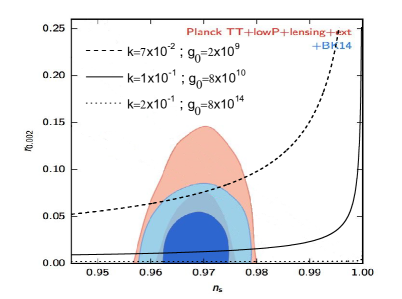
Figure 2: The evolution of the tensor to scalar ratio $r$ versus the scalar spectral index $n_{s}$(upper panel) and the evolution of the difference ${\mathcal{A}}-R$ versus the scalar spectral index $n_{s}$(lower panel) in the G-warm intermediate model for the case in which the dissipative coefficient depends of the scalar field as $\Gamma(\phi)\propto V(\phi)$. In both panels we use three different values of the pairs ($k,g_{0}$).

In the upper panel of Fig.2, we plot the tensor-to-scalar ratio $r$ against the scalar spectral index $n_{s}$, and in the lower panel we show the necessary condition of domination of the Galileon effect in which ${\mathcal{A}}\gg 1+R$ versus the scalar spectral index $n_{s}$, in the case in which the dissipation coefficient $\Gamma(\phi)\propto V(\phi)$. For both panels, we have considered three different pairs $(k,g_{0})$. The upper panel shows the two-dimensional marginalized constraints at 68$\%$ and 95$\%$ C.L. on the consistency relation $r=r(n_{s})$. The lower panel shows the evolution of the difference ${\mathcal{A}}-R$ during the inflationary scenario. Here, we make sure that the condition of domination Galileon effect in which ${\mathcal{A}}\gg 1+R$ is valid. In the upper panel we consider the consistency relation $r=r(n_{s})$ from Eq.(48). Also, in order to write down values that associate the difference ${\mathcal{A}}-R$ to the scalar spectral index $n_{s}$, we considered Eq.(50) (lower panel). To obtain the pair $(k,g_{0})$, we numerically solve Eqs.(48) and (52), in order to satisfy the constraint on the consistency relation $r=r(n_{s})<0.07$ as well as the essential condition for warm inflation to occur, $T/H>1$. In this way, the constraints on the several parameters are found to be $g_{0}>2\times 10^{9}$ and $k>7\times 10^{-2}$. Here, we have used Eqs.(47) for the value of $A$ together with the number of $e$-folds $N=60$. Analogously as before, for the specific case in which $T/H>1$ and $r=r(n_{s})<0.01$, we obtained that the lower limit for $g_{0}>8\times 10^{10}$ and $k_{0}>1\times 10^{-1}$. Similarly, for the special case in which $T/H>1$ and $r=r(n_{s})<0.0001$, we found that the lower bounds for the pair of the parameters are given by $g_{0}>8\times 10^{14}$ and $k>2\times 10^{-1}$, respectively. Here, it is worth to mention that the lower bound for the parameter $g_{0}$ is similar to the case in which the dissipative coefficient is $\Gamma_{0}=$const.

As before, from the lower plot we observe that for $g_{0}>8\times 10^{14}$ and $k>2\times 10^{-1}$, the G-warm model evolves according to the domination of the Galilean coupling, i.e. ${\mathcal{A}}\gg 1+R$. Similarly as before, we noted that for the pair $g_{0}>8\times 10^{14}$ and $k>2\times 10^{-1}$, the G-warm model is able to predict a tensor-to-scalar ratio such that $r\sim 0$. In fact, in order to satisfy the condition of domination of Galileon coupling, given by ${\mathcal{A}}\gg 1+R$, we have that $r\sim 0$. In this sense, the consistency relation $r=r(n_{s})$ does not impose any constraints on the space of parameters as the previous case.

IV General solution.

In this section we will study the general solution of G-warm intermediate inflationary model. In this sense, we will consider that the left terms of Eq.(13) are similar i.e., $R\sim{\mathcal{A}}\sim 1$, that we will call it the general solution. From the slow-roll equation of motion for the inflaton field given by Eq.(13), we can obtain an equation for $\dot{\phi}$ given by

$$\dot{\phi}^{3}+\left({1+R\over 3\,g_{0}H}\right)\dot{\phi}^{2}-{2(-\dot{H})\over 3\,g_{0}H}=0.\,$$ (53)

Here we note that this equation depends on the ratio $R=\Gamma/3H$. Thus, in the following we will analyze our model for two specific cases of the dissipation coefficient $\Gamma$. The first case we will analyze corresponds to $\Gamma(\phi)=\Gamma_{0}=$ constant and in the second case we will study the case in which $\Gamma(\phi)\propto V(\phi)$, as it was previously studied.

IV.1 Case $\Gamma=\Gamma_{0}=$ constant.

Let us consider that our model of G-warm inflation takes place for constant dissipative coefficient $\Gamma=\Gamma_{0}$ during the regime in which ${\mathcal{A}}\sim R\sim 1$. From Eq.(53) we find that the speed of the scalar field $\dot{\phi}$ can be written as

$$\dot{\phi}={3H+\Gamma_{0}\over 27g_{0}H^{2}}\left[-1+2\cosh\left({1\over 3}\cosh^{-1}\left[{3^{8}g_{0}^{2}H^{5}(-\dot{H})\over(3H+\Gamma_{0})^{3}}-1\right]\right)\right].$$ (54)

From Eq.(22) the power spectrum of the scalar perturbation results

$${\mathcal{P}_{\mathcal{R}}}={\sqrt{3}\over 2\pi^{2}}\left({\Gamma_{0}\over 4C_{\gamma}}\right)^{1\over 4}H^{11\over 4}\dot{\phi}^{-{3\over 2}}\sqrt{1+\Gamma_{0}/3H+6g_{0}H\dot{\phi}},$$ (55)

and since the scalar spectral index $n_{s}$ is given by $n_{s}-1=\frac{d\ln\,{\mathcal{P}_{R}}}{d\ln k}$, we have

$$n_{s}=1-{11\over 4}\varepsilon_{1}+{3\over 2}\epsilon_{2}^{(I)}+{1\over 2}\epsilon_{5}^{(I)},$$ (56)

where the coefficient $\epsilon_{2}^{(I)}$ is given by

$$\epsilon_{2}^{(I)}={2\ddot{H}+\dot{\phi}^{2}\dot{R}+3g_{0}\dot{H}\dot{\phi}^{3}\over 2H\dot{\phi}^{2}(1+R)+9g_{0}H^{2}\dot{\phi}^{3}},$$

and the parameter $\epsilon_{5}^{I}$ is defined as

$$\epsilon_{5}^{(I)}={-\Gamma_{0}\dot{H}/3H^{2}+6g_{0}\dot{H}\dot{\phi}+6g_{0}H\ddot{\phi}\over H(1+\Gamma_{0}/3H+6g_{0}H\dot{\phi})},\,\,\,\mbox{with}\,\,\,\,\,-\ddot{\phi}={2\ddot{H}+\dot{\phi}^{2}\dot{R}+3g_{0}\dot{H}\dot{\phi}^{3}\over 2\dot{\phi}(1+R)+9g_{0}H\dot{\phi}^{2}}.$$

Here $\dot{R}=-\Gamma_{0}H^{-2}\dot{H}/3$.

Recall that the Hubble rate in terms of the number of $e$-folds $N$ for intermediate inflation can be rewritten as $H(N)=Af\,\left[{Af\over 1+f(N-1)}\right]^{1-f\over f},$ and also $-\dot{H}(N)=Af(1-f)\,\left[{Af\over 1+f(N-1)}\right]^{2-f\over f},$ see Eqs.(18) and (19), respectively. Then, we may express both the power spectrum of the scalar perturbation ${\mathcal{P}_{\mathcal{R}}}$ and the scalar spectral index $n_{s}$ can in terms of $N$, or similarly as a function of the Hubble rate $H(N)$ in the form ${\mathcal{P}_{\mathcal{R}}}={\mathcal{P}_{\mathcal{R}}}[H(N)]$, and $n_{s}=n_{s}[H(N)],$ respectively.

Also from Eq.(25), we may write the tensor-to-scalar ratio $r$, for the full solution when $\Gamma=\Gamma_{0}=$ constant. In this form, we have

$$r\simeq{4\over\sqrt{3}}\left({4C_{\gamma}\over\Gamma_{0}}\right)^{1\over 4}H^{-3\over 4}\dot{\phi}^{{3\over 2}}(1+\Gamma_{0}/3H+6g_{0}H\dot{\phi})^{-1/2},$$ (57)

where $\dot{\phi}$ is given by Eq.(54). As before, the tensor-to-scalar ratio $r$ can be rewritten in terms of the number of $e$-folds $N$ as $r=r[H(N)]$.

Figure 3: Plot of the tensor-to-scalar ratio $r$ against the scalar spectral index $n_{s}$(upper panel)Array:2015xqh and the evolution of the function ${\mathcal{A}}+R$ versus the number of $e$-folds $N$(lower panel) in the G-warm intermediate model for $\Gamma=\Gamma_{0}=$constant, for the general solution. In both panels we use three several values of the parameter $f$ with their corresponding trios of values $(\Gamma_{0},g_{0},A)$.

In Fig.3 we show the plot of the tensor-to-scalar ratio $r$ against the scalar spectral index $n_{s}$ (upper panel). Here, we show the two-dimensional marginalized constraints at 68$\%$ and 95$\%$ C.L. on the consistency relation $r=r(n_{s})$ from BICEP2/Keck Array Collaborations dataArray:2015xqh . In the lower panel, we show ${\mathcal{A}}+R$ as a function of the number of $e$-folds $N$. In particular, it is depicted the evolution of the function ${\mathcal{A}}+R$ during the inflationary period i.e., between the number of $e$-folds $N=0$ (beginning of inflation, see Eq.(20)) and $N=70$. We also establish that the condition in which ${\mathcal{A}}\sim R\sim 1$, is satisfied, in order to be consistent with the full solution to the Klein-Gordon equation, see Eq.(13) (under slow roll approximation). In both panels we considered the case when $\Gamma=\Gamma_{0}=$ constant, and we have also fixed three different values of $f$, which characterizes the intermediate expansion law.

In order to write down values that relate $r$ and $n_{s}$, we numerically manipulate Eqs.(56) and (57) to get the consistency relation $r=r(n_{s})$ (upper plot). Analogously, to relate the effective function ${\mathcal{A}}+R$ to the number of $e$-folds $N$ between $N=0$ to $N=70$ during the inflationary stage, we numerically utilize Eqs.(18), (19) and (54), see the lower panel. In order to obtain the trio of parameters $(\Gamma_{0},g_{0},A)$ for fixed value of parameter $f$, which characterizes the intermediate expansion law , we consider the last data Planck collaboration Akrami:2018odb , which set the power spectrum of the scalar perturbation to ${\mathcal{P}_{\mathcal{R}}}\simeq 2.2\times 10^{-9}$, and the scalar spectral index to $n_{s}\simeq 0.964$, and we also consider the minimum condition for warm inflation to occur, $T/H=1$ . Here, we have fixed the number of $e$-folds to $N=60$. In this sense, the corresponding trio of values $(\Gamma_{0},g_{0},A)$ for $f=0.58$, is found to be $(4.9\times 10^{-11},2.7\times 10^{8},1.2\times 10^{-2})$. Analogously for the value $f=0.59$, we obtained $(2.3\times 10^{-11},1.4\times 10^{10},8.6\times 10^{-3})$. In a similarly fashion, for $f=0.6$ we determined that the trio of values is given by $(7.9\times 10^{-12},2.6\times 10^{11},5.4\times 10^{-3})$.

From the lower panel of Fig.3, we observe that in order to satisfy the condition ${\mathcal{A}}\sim R\sim 1$ given by the full Klein-Gordon equation (see (13)), we obtain that the upper limit for the parameter $f$ is given by $f<0.6$. In this context, we note that for values of $f>0.6$, the effective function ${\mathcal{A}}+R\gg 0$, during the inflationary epoch, and the model does not evolves in agreement to the general regime ${\mathcal{A}}\sim R\sim 1$. However, from the upper panel we note that the upper bound for $f$ is given by $f<0.6$, since the model is well supported by the Planck data from the consistency relation $r=r(n_{s})$. Here, both conditions are satisfied. We also mentioned that, according to the parameter $f$ increases, the corresponding values for the parameters $\Gamma_{0}$ and $A$ decrease, however the parameter $g_{0}$ increase.

IV.2 Case $\Gamma(\phi)\propto V(\phi)$

Now we assume that our G-model of warm inflation takes place for dissipative coefficient being a function of the scalar field $\phi$ given by $\Gamma(\phi)=kV(\phi)$, during the regime in with ${\mathcal{A}}\sim R\sim 1$, i.e. the full Klein-Gordon equation (13) under slow-roll approximation. In this way, from Eq.(53) we find that $\dot{\phi}$ can be written as

$$\dot{\phi}={1+kH\over 9g_{0}H}\left[-1+2\cosh\left({1\over 3}\cosh^{-1}\left[{3^{5}g_{0}^{2}H^{2}(-\dot{H})\over(1+kH)^{3}}-1\right]\right)\right].$$ (58)

For this dissipative coefficient, the power spectrum of the scalar perturbation ${\mathcal{P}_{\mathcal{R}}}$, yields

$${\mathcal{P}}_{\mathcal{R}}={\sqrt{3}\over 2\pi^{2}}\left({3k\over 4C_{\gamma}}\right)^{1\over 4}H^{13\over 4}\dot{\phi}^{-{3\over 2}}\sqrt{1+kH+6g_{0}H\dot{\phi}}.$$ (59)

Thus, we obtain that the scalar spectral index $n_{s}$ results in

$$n_{s}=1-{13\over 4}\varepsilon_{1}+{3\over 2}\epsilon_{2}^{(II)}+{1\over 2}\epsilon_{5}^{(II)},$$ (60)

where $\epsilon_{2}^{(II)}$ is defined as

$$\epsilon_{2}^{(II)}=\epsilon_{2}^{(I)}={2\ddot{H}+\dot{\phi}^{2}\dot{R}+3g_{0}\dot{H}\dot{\phi}^{3}\over 2H\dot{\phi}^{2}(1+R)+9g_{0}H^{2}\dot{\phi}^{3}},\,\,\,\mbox{with}\,\,\,\,\dot{R}=k\dot{H},$$

and the parameter $\epsilon_{5}^{(II)}$ is given by

$$\epsilon_{5}^{(II)}={k\dot{H}+6g\dot{H}\dot{\phi}+6gH\ddot{\phi}\over H(1+kH+6g_{0}H\dot{\phi})}.$$

Here $\dot{\phi}$ corresponds to Eq.(58) and $\ddot{\phi}$ is given by $\ddot{\phi}=-\left[{2\ddot{H}+\dot{\phi}^{2}\dot{R}+3g_{0}\dot{H}\dot{\phi}^{3}\over 2\dot{\phi}(1+R)+9g_{0}H\dot{\phi}^{2}}\right]$.

As before, we find that the tensor-to-scalar ratio $r$, for the full solution when $\Gamma(\phi)\propto V(\phi)$ becomes

$$r\simeq{4\over\sqrt{3}}\left({4C_{\gamma}\over 3k}\right)^{1\over 4}H^{-5\over 4}\dot{\phi}^{{3\over 2}}(1+kH+6g_{0}H\dot{\phi})^{-1/2}.$$ (61)

Here we have used Eq.(25). As in the previous case, we can rewrite the power spectrum of the scalar perturbation ${\mathcal{P}_{\mathcal{R}}}$, the scalar spectral index $n_{s}$ and the tensor-to-scalar ratio $r$ in terms of the number of $e$-folds $N$, or similarly as a function of the Hubble rate $H(N)$ in the form ${\mathcal{P}_{\mathcal{R}}}={\mathcal{P}_{\mathcal{R}}}[H(N)]$, $n_{s}=n_{s}[H(N)]$ and $r=r[H(N)]$.

Analogously as before, in Fig.4 we show the tensor-to-scalar ratio $r$ versus the scalar spectral index $n_{s}$ (upper panel). Here, we show the two-dimensional marginalized constraints at 68$\%$ and 95$\%$ C.L. on the consistency relation $r=r(n_{s})$ from Ref.Array:2015xqh . In the lower panel we show the function ${\mathcal{A}}+R$ versus the number of $e$-folds $N$. In this panel we exhibit the evolution of the function ${\mathcal{A}}+R$ during the inflationary period between the number of $e$-folds $N=0$ and $N=70$. We also check that the condition ${\mathcal{A}}\sim R\sim 1$ is satisfied, in order to obtain the full expression to the Klein-Gordon equation (13) under slow-roll approximation. In both panels we considered that $\Gamma(\phi)\propto V(\phi)$ as well as three different values of the parameter $f$ .

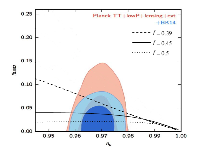
Figure 4: The tensor-to-scalar ratio $r$ as a function of the scalar spectral index $n_{s}$Array:2015xqh (upper panel) and the evolution of the ${\mathcal{A}}+R$ in terms the number of $e$-folds $N$(lower panel) in the G-warm intermediate model when $\Gamma(\phi)\propto V(\phi)$ for the general solution. In both panels we use three different values of the parameter $f$.

As before, by manipulating numerically Eqs.(60) and (61), we obtain the consistency relation $r=r(n_{s})$ for the upper plot. Analogously, for the function ${\mathcal{A}}+R$ versus the number of $e$-folds $N$, we numerically considered Eqs.(18), (19) and (58) in order to plot ${\mathcal{A}}+R$ against $n_{s}$ (lower panel).

Since the parameter $f$ lies in the range $0<f<1$, we fixed the valuer of $f$, in order to obtain the trio of values $(k,g_{0},A)$. Then, we numerically utilize Eqs.(16),(59) and (60) to satisfy the minimum condition for that warm inflation takes place in which $T/H=1$, the power spectrum of the scalar perturbation ${\mathcal{P}_{\mathcal{R}}}=2.2\times 10^{-9}$ and the scalar spectral index $n_{s}=0.964$ for a given value of $f$. In particular, by fixing the number of $e$-folds to $N=60$, together with $T/H(N=60)=1$, ${\mathcal{P}_{\mathcal{R}}}(N=60)=2.2\times 10^{-9}$, $n_{s}(N=60)=0.964$ and $f$=0.39, we find numerically that the trio of values of $(k,g_{0},A)$ is given by $(0.5,3.3\times 10^{6},0.3)$. Analogously, for $f=0.45$, we obtained numerically the trio $(0.6,8.7\times 10^{8},0.1)$. Similarly, for $f=0.5$ we determined that the trio corresponds to $(0.9,5.2\times 10^{9},4.1\times 10^{-2})$.

From the upper panel of Fig.4, we observe that the upper bound for $f$ becomes $f<0.39$, since the model is well supported by the Planck data in $n_{s}-r$ plane. However, from the lower panel we note that in order to satisfy the condition ${\mathcal{A}}\sim R\sim 1$ (in the full Klein-Gordon equation (13)), the upper limit for the parameter $f$ is found to be $f<0.5$. In this context, we determine that for values of $f>0.5$, the effective function becomes ${\mathcal{A}}+R\gg 0$ during inflation, hence the model does not evolves according to the condition ${\mathcal{A}}\sim R\sim 1$. Numerically, we also noted if the parameter $f$ increases, both the associated parameters with the dissipative coefficient, $k$ and the coupling parameter $g_{0}$ increase, while the associated parameter to the intermediate expansion $A$ decreases. It is interesting to highlight that the allowed ranges for the parameters $f$, $k$, $g_{0}$ and $A$ for the full model are found only from the condition in which the full-model evolves according to ${\mathcal{A}}\sim R\sim 1$. In this form, we find that the consistency relation $r=r(n_{s})$ does not impose any constraints on the parameters for this model.

V Conclusions

In this paper we have investigated the realization of the intermediate inflationary model in G-warm inflation scenario. By assuming the Galileon term under the slow roll-approximation, we have considered the coupling function as $G(\phi,X)=g_{0}X$, where $g_{0}=$ constant, for two different dissipation coefficients in the scenario of intermediate warm inflation. In particular, we have studied two expressions for the dissipative coefficient, namely $\Gamma=\Gamma_{0}=$ constant and $\Gamma(\phi)\propto V(\phi)$. In addition, we have assumed that the dynamics takes place according two regimes. In the first one, we have considered the domination of the Galilean coupling over the standard terms of warm inflation. In the second regime, we have considered that all terms become of the same order in the slow-roll equation for the scalar field. By assuming the intermediate expansion law, we have found analytical solutions to the background equations under the slow-roll approximation for each regime, considering the two expressions for the dissipative coefficient. Also, for both regimes, we have found the constraints on the several parameters, assuming the last data of Planck in addition to the condition of domination term associated with its regime.

In order to developed the analysis for the first regime, or domination of the Galileon term i.e. ${\cal{A}}\gg 1+\Gamma/3H$, we have set the parameter $f$ from the expression for scalar spectral index and the parameter $A$ from the amplitude of the power spectrum of scalar perturbations. In order to obtain the parameters characterizing the coupling $G(\phi,X)$ and the dissipative coefficient $\Gamma$, such as $g_{0}$ and $\Gamma_{0}$ (or the pair $(g_{0},k)$), we have solved numerically the conditions for warm inflation, i.e. $T>H$ and the consistency relation $r=r(n_{s})<0.07$ from last data of Planck. Thus, for the regime in which the domination of warm inflation comes from the Galilean coupling, we have obtained the constraints on the parameters of our model, which only come from the condition ${\cal{A}}\gg 1+\Gamma/3H$, giving a lower bound on the parameter-space.

In this sense, the consistency relation $r=r(n_{s})$ does not impose any constraints on the parameters, since the tensor-to-scalar ratio $r\sim 0$ for the allowed range of parameters. We have found that the lower bound on the parameter $g_{0}$ is similar to the different types of dissipation coefficients; $\Gamma=\Gamma_{0}=$constant and $\Gamma\propto V(\phi)$ during for regime in which ${\cal{A}}\gg 1+\Gamma/3H$.

In the second stage of the analysis of our model, we consider the dynamics takes place in the so-called general regime of Eq.(53) (considering slow-roll approximation). Here, we have fixed the parameter $f$ associated to the intermediate expansion $f$ which lies in the range $0<f<1$. Also, in order to find the other parameters, such $A$, from the intermediate expansion law, the coupling of $G(\phi,X)$ and the ones which characterize the dissipative coefficient $\Gamma$, namely $g_{0}$ and $\Gamma_{0}$ (or the pair $(g_{0},k)$), we have solved numerically the conditions for warm inflation in which the temperature $T=H$, and the consistency relation in which $r=r(n_{s})<0.07$ from last data of Planck. For the several expression for the dissipative coefficient, we have found that the current observational data of Planck does not impose any constraints on the space of parameters. On the other hand, we have found that only the condition for the model evolves according to $R\sim 1\sim\cal{A}$ is able to impose the constraints on the parameters characterizing our model. In this sense, we have found that these models are well supported by the last Planck data , since the tensor-to-scalar ratio $r<0.07$. Also, due to the difficulty in treating the equations analytically, we have the study of this regime (general solution) in numerical way.

As a final remark, we have not studied G-warm inflation in the framework of intermediate expansion when the coupling function $g$ has a dependence on the inflaton, as neither a dissipative coefficient having a dependence on the temperature of the thermal bath $T$, i.e., $\Gamma(\phi,T)$. We hope to be able to address these points in a future work.