Robust $H_{\infty}$ kinematic control of manipulator robots using dual quaternion algebra

Abstract

This paper proposes a robust dual-quaternion based $H_{\infty}$ task-space kinematic controller for robot manipulators. To address the manipulator liability to modeling errors, uncertainties, exogenous disturbances, and their influence upon the kinematics of the end-effector pose, we adapt $H_{\infty}$ techniques—suitable only for additive noises—to unit dual quaternions. The noise to error attenuation within the $H_{\infty}$ framework has the additional advantage of casting aside requirements concerning noise distributions, which are significantly hard to characterize within the group of rigid body transformations. Using dual quaternion algebra, we provide a connection between performance effects over the end-effector trajectory and different sources of uncertainties and disturbances while satisfying attenuation requirements with minimum instantaneous control effort. The result is an easy-to-implement closed form $H_{\infty}$ control design criterion. The performance of the proposed strategy is evaluated within different realistic simulated scenarios and validated through real experiments.

1 Introduction

To ensure adequate performance, robot task-space kinematic controllers must ensure robustness against modeling errors, uncertainties, and exogenous disturbances that affect the end-effector pose. To cope with the challenges that arise from the pose description and possible representation singularities, the coupled translation and rotation kinematics can be modeled using non-minimal representations such as homogeneous transformation matrices (HTM) and unit dual quaternions. The unit dual quaternion is a non-singular representation for rigid transformations that is more compact, efficient and less computationally demanding than HTM (Aspragathos and Dimitros, 1998). In addition, dual quaternion algebra can represent rigid motions, twists, wrenches and several geometrical primitives in a straightforward way, which is useful when describing geometrical tasks directly in the task-space (Marinho et al., 2019). Moreover, control laws are defined directly over a vector field, eliminating the need to extract additional parameters or to design matrix-based controllers.

Thanks to those advantages, there has been an increasing interest in the study of kinematic representation and control in dual quaternion space. Those works comprise rigid motion stabilization, tracking, and multiple body coordination (Han et al., 2008; Wang et al., 2012; Wang and Yu, 2013; Mas and Kitts, 2017), and kinematic control of manipulators with single and multiple arms and human-robot interaction (Adorno et al., 2010; Figueredo et al., 2013; Adorno et al., 2015).

Despite the developments on robot control using dual quaternion algebra, there is still a gap in existing literature concerning the influence of control parameters, uncertainties, and disturbances over tracking robustness and performance when the trajectory is represented by unit dual quaternions.

1.1 Statement of contributions

We propose a robust dual-quaternion based $H_{\infty}$ task-space kinematic controller for manipulators. The new method directly connects different sources of uncertainties and disturbances to their corresponding performance effects over the end-effector trajectory in dual quaternion space. The controller explicitly addresses the influence of such disturbances over the end-effector pose, in the $H_{\infty}$ sense, which does not require detailed knowledge about the statistical distribution of disturbances. This is paramount as those distributions are significantly hard to characterize within the group $\text{Spin}(3)\ltimes\mathbb{R}^{3}$ of unit dual quaternions (or even $SE(3)$). Using dual quaternion algebra, we derive easy-to-implement closed form $H_{\infty}$ control and tracking strategies at the end-effector level that incorporate robustness requirements, disturbance attenuation and performance properties over the pose kinematics, while minimizing the required control effort. In summary, the contributions to the state of the art are:

1. Introduction of novel geometrical description of disturbances within the space of unit dual quaternions;

2. Development of an easy-to-implement, closed form $H_{\infty}$ controller for end-effector trajectory tracking.

2 Preliminaries

The algebra of quaternions is generated by the basis elements $1,\hat{\imath},\hat{\jmath},$ and $\hat{k}$ and a distributive multiplication operation satisfying $\hat{\imath}^{2}{=}\hat{\jmath}^{2}{=}\hat{k}^{2}{=}\hat{\imath}\hat{\jmath}\hat{k}{=}-1$, yielding the set

$$\mathbb{H}\triangleq\smash{\left\{\eta+\mu_{1}\hat{\imath}+\mu_{2}\hat{\jmath}+\mu_{3}\hat{k}\,:\,\eta,\mu_{1},\mu_{2},\mu_{3}\in\mathbb{R}\right\}}.$$

An element $\boldsymbol{h}=\eta+\mu_{1}\hat{\imath}+\mu_{2}\hat{\jmath}+\mu_{3}\hat{k}\in\mathbb{H}$ may be decomposed into real and imaginary components $\operatorname{\mathrm{Re}}\left(\boldsymbol{h}\right)\triangleq\eta$ and $\operatorname{\mathrm{Im}}\left(\boldsymbol{h}\right)\triangleq\mu_{1}\hat{\imath}+\mu_{2}\hat{\jmath}+\mu_{3}\hat{k}$, such that $\boldsymbol{h}=\operatorname{\mathrm{Re}}\left(\boldsymbol{h}\right)+\operatorname{\mathrm{Im}}\left(\boldsymbol{h}\right)$.

Quaternion elements with real part equal to zero belong to the set of pure quaternions $\mathbb{H}_{p}\triangleq\left\{\boldsymbol{h}\in\mathbb{H}\ :\operatorname{\mathrm{Re}}\left(\boldsymbol{h}\right)\right.$ $\left.=0\right\}$, and are equivalent to vectors in $\mathbb{R}^{3}$ under the addition operation and the bijective operator $\operatorname{vec}_{3}:\mathbb{H}_{p}{\rightarrow}\mathbb{R}^{3}$, such that $\boldsymbol{\mu}{=}\mu_{1}\hat{\imath}+\mu_{2}\hat{\jmath}+\mu_{3}\hat{k}$ yields $\operatorname{vec}_{3}\boldsymbol{\mu}{=}\begin{bmatrix}\mu_{1}&\mu_{2}&\mu_{3}\end{bmatrix}^{T}$. The inverse mapping is given by the operator $\underline{\operatorname{vec}}_{3}$.

The set of unit quaternions is defined as $\mathbb{S}^{3}\triangleq\{\boldsymbol{h}\in\mathbb{H}\,:\,\left\|\boldsymbol{h}\right\|=1\}$, where $\left\|\boldsymbol{h}\right\|\triangleq\sqrt{\boldsymbol{h}\boldsymbol{h}^{\ast}}=\sqrt{\boldsymbol{h}^{\ast}\boldsymbol{h}}$ is the quaternion norm and $\boldsymbol{h}{}^{\ast}\triangleq\operatorname{\mathrm{Re}}\left(\boldsymbol{h}\right)-\operatorname{\mathrm{Im}}\left(\boldsymbol{h}\right)$ is the conjugate of $\boldsymbol{h}$. The set $\mathbb{S}^{3}$, together with the multiplication operation, forms the Lie group of unit quaternions, $\mathrm{Spin}\left(3\right)$, whose identity element is $1$ and the inverse of any element $\boldsymbol{h}\in\mathrm{Spin}\left(3\right)$ is $\boldsymbol{h}^{\ast}$. An arbitrary rotation angle $\phi\in\mathbb{R}$ around the rotation axis $\boldsymbol{n}\in\mathbb{H}_{p}\cap\mathbb{S}^{3}$, with $\boldsymbol{n}=n_{x}\hat{\imath}+n_{y}\hat{\jmath}+n_{z}\hat{k}$, is represented by $\boldsymbol{r}=\cos(\phi/2)+\sin(\phi/2)\boldsymbol{n}\in\mathrm{Spin}\left(3\right)$ (Selig, 2005).

The complete rigid body displacement, in which translation and rotation are coupled, is similarly described using dual quaternion algebra (Selig, 2005). The dual quaternion set is given by the set

$$\mathcal{H}\triangleq\{\boldsymbol{h}+\varepsilon\boldsymbol{h}^{\prime}\,:\,\boldsymbol{h},\boldsymbol{h}^{\prime}\in\mathbb{H},\ \varepsilon^{2}=0,\ \varepsilon\neq 0\},$$

where $\varepsilon$ is the dual unit. Given $\underline{\boldsymbol{h}}=\boldsymbol{h}+\varepsilon\boldsymbol{h}^{\prime}\in\mathcal{H}$, its norm is defined as $\left\|\underline{\boldsymbol{h}}\right\|\triangleq\sqrt{\underline{\boldsymbol{h}}\underline{\boldsymbol{h}}^{*}}=\sqrt{\underline{\boldsymbol{h}}^{*}\underline{\boldsymbol{h}}}$ and the element $\underline{\boldsymbol{h}}^{*}\triangleq\boldsymbol{h}^{*}+\varepsilon\boldsymbol{h}^{\prime*}$ is the conjugate of $\underline{\boldsymbol{h}}$. Under multiplication, the subset of unit dual quaternions $\underline{\boldsymbol{\mathcal{S}}}\triangleq\{\underline{\boldsymbol{h}}\in\mathcal{H}\,:\,\left\|\underline{\boldsymbol{h}}\right\|=1\}$ forms the Lie group $\text{Spin}(3)\ltimes\mathbb{R}^{3}$, whose identity element is $1$ and the group inverse of $\underline{\boldsymbol{x}}\in\text{Spin}(3)\ltimes\mathbb{R}^{3}$ is $\underline{\boldsymbol{x}}^{\ast}$ (Selig, 2005). An arbitrary rigid displacement defined by a translation $\boldsymbol{p}\in\mathbb{H}_{p}$ followed by a rotation $\boldsymbol{r}\in\mathbb{S}^{3}$ is represented in $\text{Spin}(3)\ltimes\mathbb{R}^{3}$ by the element $\underline{\boldsymbol{x}}=\boldsymbol{r}+(1/2)\varepsilon\boldsymbol{p}\boldsymbol{r}$.

The first order kinematic equation of a rigid body motion is described by

$$\dot{\underline{\boldsymbol{x}}}=\smash{\frac{1}{2}}\underline{\boldsymbol{\xi}}\underline{\boldsymbol{x}},$$ (1)

where $\underline{\boldsymbol{\xi}}=\boldsymbol{\omega}+\varepsilon\left(\dot{\boldsymbol{p}}+\boldsymbol{p}\times\boldsymbol{\omega}\right)$ is the twist in the inertial frame and $\boldsymbol{\omega},\dot{\boldsymbol{p}}\in\mathbb{H}_{p}$ are the angular and linear velocities, respectively. The twist $\underline{\boldsymbol{\xi}}$ belongs to the set of pure dual quaternions, defined as $\mathcal{H}_{p}\triangleq\{\left(\boldsymbol{h}+\varepsilon\boldsymbol{h}^{\prime}\right)\in\mathcal{H}\,:\,\operatorname{\mathrm{Re}}\left(\boldsymbol{h}\right){=}\operatorname{\mathrm{Re}}\left(\boldsymbol{h}^{\prime}\right){=}0\}$, which is equivalent to vectors in $\mathbb{R}^{6}$ under the addition operation and the bijective operator $\operatorname{vec}_{6}:\mathcal{H}_{p}\rightarrow\mathbb{R}^{6}$, such that $\underline{\boldsymbol{\xi}}=(\xi_{1}\hat{\imath}+\xi_{2}\hat{\jmath}+\xi_{3}\hat{k})+\varepsilon(\xi_{4}\hat{\imath}+\xi_{5}\hat{\jmath}+\xi_{6}\hat{k})$ yields $\operatorname{vec}_{6}\underline{\boldsymbol{\xi}}=\begin{bmatrix}\xi_{1}&{\cdots}&\xi_{6}\end{bmatrix}^{T}$. The inverse mapping is denoted by $\underline{\operatorname{vec}}_{6}:\mathbb{R}^{6}\rightarrow\mathcal{H}_{p}$.

2.1 Forward Kinematics of Serial Manipulators

The rigid transformation from the robot’s fixed base to its end-effector pose—i.e., its forward kinematics—is described by $\underline{\boldsymbol{x}}_{N}\left(\boldsymbol{q}\right)=\underline{\boldsymbol{x}}_{1}^{0}\underline{\boldsymbol{x}}_{2}^{1}\dots\underline{\boldsymbol{x}}_{n}^{n-1}$, with $\boldsymbol{q}{=}\begin{bmatrix}q_{1}&{\cdots}&q_{n}\end{bmatrix}^{T}$, where $\underline{\boldsymbol{x}}_{i+1}^{i}\triangleq\underline{\boldsymbol{x}}_{i+1}^{i}\left(q_{i+1}\right)\in\mathrm{Spin}\left(3\right)\ltimes\mathbb{R}^{3}$ represents the rigid transformation between the extremities of links $i$ and $i+1$ and is a function of joint configuration $q_{i+1}\in\mathbb{R}$.

The differential forward kinematics, which describes the mapping between the joints velocities and the end-effector (generalized) velocity is given by (Adorno, 2011)

$$\dot{\underline{\boldsymbol{x}}}_{N} =\frac{1}{2}\underline{\boldsymbol{\xi}}_{N}\underline{\boldsymbol{x}}_{N}=\frac{1}{2}{\sum}_{i=1}^{n}\underline{\boldsymbol{\jmath}}_{i}\dot{q}_{i}\underline{\boldsymbol{x}}_{N},$$ (2)

$$\underline{\boldsymbol{\jmath}}_{i} =2\underline{\boldsymbol{x}}_{i-1}^{0}\frac{d\underline{\boldsymbol{x}}_{i}^{i-1}}{dq_{i}}\left(\underline{\boldsymbol{x}}_{i}^{i-1}\right)^{*}\underline{\boldsymbol{x}}_{0}^{i-1}.$$ (3)

3 Uncertainties and Exogenous Disturbances

In practice, the end-effector trajectory is likely to be influenced by different sources of exogenous disturbances and inaccuracies in the manipulator’s geometrical parameters, resulting in an uncertain differential forward kinematics. To improve accuracy and control performance, the influence of those uncertainties and disturbances over the system must be explicitly regarded. Thus, we investigate two sources of disturbances, namely twist and pose uncertainties.

Twist uncertainties may be caused by exogenous disturbances that directly influence the end-effector velocity, such as unmodeled time-varying uncertainties, aerodynamic forces acting on non-rigid manipulators, and the effects of discrete implementations of controllers designed in continuous time. The differential forward kinematics under the influence of a twist disturbance $\underline{\boldsymbol{v}}_{w}$ is modeled by

$$\dot{\underline{\boldsymbol{x}}}_{N}=\frac{1}{2}{\sum}_{i=1}^{n}\underline{\boldsymbol{\jmath}}_{i}\dot{q}_{i}\underline{\boldsymbol{x}}_{N}+\frac{1}{2}\underline{\boldsymbol{v}}_{w}\underline{\boldsymbol{x}}_{N}.$$ (4)

Pose uncertainties, which are related to the end-effector pose, may also arise from unforeseen inaccuracies within model geometric parameters and time-varying uncertainties, but also comprise inaccuracies in the location of the reference frame. They can also appear due to the unmodeled parameters of the dynamic model, e.g., the gravity effect on the robot. Because they affect the forward kinematics, pose uncertainties can be mapped to (2)–(4) as

$$\underline{\boldsymbol{x}}=\underline{\boldsymbol{x}}_{N}\underline{\boldsymbol{c}},$$ (5)

where $\underline{\boldsymbol{c}}\in\mathrm{Spin}\left(3\right)\ltimes\mathbb{R}^{3}$ and $\underline{\boldsymbol{x}}$ denotes the real pose of the disturbed end-effector. The time derivative of (5) yields

$$\dot{\underline{\boldsymbol{x}}} =\dot{\underline{\boldsymbol{x}}}_{N}\underline{\boldsymbol{c}}+\underline{\boldsymbol{x}}_{N}\dot{\underline{\boldsymbol{c}}}=\frac{1}{2}{\sum}_{i=1}^{n}\underline{\boldsymbol{\jmath}}_{i}\dot{q}_{i}\underline{\boldsymbol{x}}+\frac{1}{2}\underline{\boldsymbol{v}}_{w}\underline{\boldsymbol{x}}+\frac{1}{2}\underline{\boldsymbol{x}}\bar{\underline{\boldsymbol{v}}}_{c},$$

where $\bar{\underline{\boldsymbol{v}}}_{c}\in\mathcal{H}_{p}$ is the twist related to $\dot{\underline{\boldsymbol{c}}}$, but expressed in the local frame; that is, $\dot{\underline{\boldsymbol{c}}}=\left(1/2\right)\underline{\boldsymbol{c}}\bar{\underline{\boldsymbol{v}}}_{c}$. Since the disturbance $\bar{\underline{\boldsymbol{v}}}_{c}$ can be expressed in the inertial frame by means of the norm-preserving transformation $\bar{\underline{\boldsymbol{v}}}_{c}=\underline{\boldsymbol{x}}^{*}\underline{\boldsymbol{v}}_{c}\underline{\boldsymbol{x}}$, the actual differential forward kinematics, under twist and pose uncertainties, is described by

$$\dot{\underline{\boldsymbol{x}}}=\smash{\frac{1}{2}}{\sum}_{i=1}^{n}\underline{\boldsymbol{\jmath}}_{i}\dot{q}_{i}\underline{\boldsymbol{x}}+\smash{\frac{1}{2}}\underline{\boldsymbol{v}}_{w}\underline{\boldsymbol{x}}+\smash{\frac{1}{2}}\underline{\boldsymbol{v}}_{c}\underline{\boldsymbol{x}}.$$ (6)

3.1 Tracking Error Definition

Given a desired differentiable pose trajectory $\underline{\boldsymbol{x}}_{d}\left(t\right)\in\mathrm{Spin}\left(3\right)\ltimes\mathbb{R}^{3}$, we seek to guarantee internal stability and tracking performance in terms of the noise-to-output influence over the end-effector trajectory. From (1), $\underline{\boldsymbol{x}}_{d}\left(t\right)$ satisfies the first order kinematic equation

$$\dot{\underline{\boldsymbol{x}}}_{d}=\smash{\frac{1}{2}}\underline{\boldsymbol{\xi}}_{d}\underline{\boldsymbol{x}}_{d}.$$ (7)

We define the spatial difference in $\text{Spin}(3)\ltimes\mathbb{R}^{3}$ as

$$\tilde{\underline{\boldsymbol{x}}}\triangleq\underline{\boldsymbol{x}}\underline{\boldsymbol{x}}_{d}^{\ast}=\tilde{\boldsymbol{r}}+\varepsilon\smash{\frac{1}{2}}\tilde{\boldsymbol{p}}\tilde{\boldsymbol{r}},$$ (8)

where $\tilde{\boldsymbol{r}}=\boldsymbol{r}\boldsymbol{r}_{d}^{\ast}$ denotes the orientation error in $\mathrm{Spin}\left(3\right)$ given the desired orientation $\boldsymbol{r}_{d}$, and $\tilde{\boldsymbol{p}}=\boldsymbol{p}-\tilde{\boldsymbol{r}}\boldsymbol{p}_{d}\tilde{\boldsymbol{r}}^{\ast}$ denotes the translational error in $\mathbb{H}_{p}$ given the desired position $\boldsymbol{p}_{d}$.

From (6) and (7), the error kinematics is given by

$$\dot{\tilde{\underline{\boldsymbol{x}}}} =\dot{\underline{\boldsymbol{x}}}\underline{\boldsymbol{x}}{}_{d}^{\ast}+\underline{\boldsymbol{x}}\dot{\underline{\boldsymbol{x}}}_{d}^{\ast}=\frac{1}{2}\left(\sum_{i=1}^{n}\underline{\boldsymbol{\jmath}}_{i}\dot{q}_{i}+\underline{\boldsymbol{v}}_{w}+\underline{\boldsymbol{v}}_{c}\right)\tilde{\underline{\boldsymbol{x}}}-\frac{1}{2}\tilde{\underline{\boldsymbol{x}}}\underline{\boldsymbol{\xi}}_{d}$$

$$=\frac{1}{2}\left(\underline{\operatorname{vec}}_{6}\left(\boldsymbol{J}\dot{\boldsymbol{q}}\right)+\underline{\boldsymbol{v}}_{w}+\underline{\boldsymbol{v}}_{c}\right)\tilde{\underline{\boldsymbol{x}}}-\frac{1}{2}\tilde{\underline{\boldsymbol{x}}}\underline{\boldsymbol{\xi}}_{d},$$ (9)

where $\boldsymbol{q}=\smash{\begin{bmatrix}q_{1}&\cdots&q_{n}\end{bmatrix}^{T}}$ is the measured vector of joint variables and $\boldsymbol{J}=\begin{bmatrix}\operatorname{vec}_{6}\underline{\boldsymbol{\jmath}}_{1}&\cdots&\operatorname{vec}_{6}\underline{\boldsymbol{\jmath}}_{n}\end{bmatrix}$ is the analytical Jacobian that maps the joints velocities $\dot{\boldsymbol{q}}$ to the (undisturbed) twist $\operatorname{vec}_{6}\underline{\boldsymbol{\xi}}_{N}$ of the end-effector.

From the spatial difference (8), we define a right invariant dual quaternion error function

$$\tilde{\underline{\boldsymbol{z}}}\triangleq 1-\tilde{\underline{\boldsymbol{x}}}=\tilde{\boldsymbol{z}}+\varepsilon\tilde{\boldsymbol{z}}^{\prime}$$ (10)

with dynamics described by $\dot{\tilde{\underline{\boldsymbol{z}}}}=-\dot{\tilde{\underline{\boldsymbol{x}}}}$. Therefore, $\tilde{\underline{\boldsymbol{z}}}\rightarrow 0$ implies $\tilde{\underline{\boldsymbol{x}}}\rightarrow 1$, which implies $\underline{\boldsymbol{x}}\rightarrow\underline{\boldsymbol{x}}_{d}$.

To address the detrimental influence of the uncertainties and disturbances in system (9), we address as variable of interest the orientation and position errors from (8) and (10), defined respectively as

$$\operatorname{\mathcal{\mathscr{O}}\negmedspace}\left(\tilde{\underline{\boldsymbol{z}}}\right) \triangleq\operatorname{\mathrm{Im}}\left(\tilde{\boldsymbol{z}}\right), \operatorname{\mathscr{T}\negmedspace}\left(\tilde{\underline{\boldsymbol{z}}}\right) \triangleq-2\tilde{\boldsymbol{z}}^{\prime}(1{-}\tilde{\boldsymbol{z}}^{\ast})=\tilde{\boldsymbol{p}}.$$ (11)

3.2 Performance Under Uncertainties and Disturbances

The tracking error defined in the previous subsection explicitly accounts for uncertainties and noises in the closed-loop control of the robotic arm, allowing a performance assessment for any control strategy. If the statistics of the uncertainties and noises are available, a stochastic analysis can be considered (Simon, 2006). However, for non-Euclidean spaces the probability density functions are, in general, hard to characterize and, when available, difficult to manipulate. In this paper, we propose a deterministic performance analysis based on the $H_{\infty}$ approach (Abu-Khalaf et al., 2006), in which the effect of the input onto the output is intuitively measured as a maximal level of amplification. The main advantage is the needlessness for assumptions regarding the statistics of the uncertainties and noises. As a result, the analysis is simpler than the stochastic one.

The following definition describes the robust performance (in the $H_{\infty}$ sense) in terms of the dual quaternion error (10) and the disturbances $\underline{\boldsymbol{v}}_{w}=\boldsymbol{v}_{w}+\varepsilon\boldsymbol{v}_{w}^{\prime}$ and $\underline{\boldsymbol{v}}_{c}=\boldsymbol{v}_{c}+\varepsilon\boldsymbol{v}_{c}^{\prime}$, assuming $\boldsymbol{v}_{w},\boldsymbol{v}_{w}^{\prime},\boldsymbol{v}_{c},\boldsymbol{v}_{c}^{\prime}\in L_{2}([0,\infty),\mathbb{H}_{p})$.

Definition 1.

For ${\gamma_{{}_{\mathcal{O}}}}_{1},{\gamma_{{}_{\mathcal{O}}}}_{2},{\gamma_{{}_{\mathcal{T}}}}_{1},{\gamma_{{}_{\mathcal{T}}}}_{2}\in\left(0,\infty\right)$, the robust control performance is achieved, in the $H_{\infty}$ sense, if the following hold (Abu-Khalaf et al., 2006)

(1) The error (10) is exponentially stable for $\underline{\boldsymbol{v}}_{w}{=}\underline{\boldsymbol{v}}_{c}{=}0$;

(2) Under the assumption of zero initial conditions, the disturbances’ influence upon the attitude and translation errors is attenuated below a desired level; that is, $\forall\left(\boldsymbol{v}_{w},\boldsymbol{v}_{c},\boldsymbol{v}_{w}^{\prime},\boldsymbol{v}_{c}^{\prime}\right)\in L_{2}((0,\infty),\mathbb{H}_{p})$

$$\begin{aligned} \int_{0}^{\infty}\negthickspace\negthickspace\negthickspace\left\|\operatorname{\mathcal{\mathscr{O}}\negmedspace}\left(\tilde{\underline{\boldsymbol{z}}}\left(t\right)\right)\right\|^{2}\negthickspace dt&\leq{\gamma_{{}_{\mathcal{O}}}}_{1}^{\negthickspace\negthickspace 2}\int_{0}^{\infty}\negthickspace\negthickspace\negthickspace\left\|\boldsymbol{v}_{w}\left(t\right)\right\|^{2}\negthickspace dt+{\gamma_{{}_{\mathcal{O}}}}_{2}^{\negthickspace\negthickspace 2}\int_{0}^{\infty}\negthickspace\negthickspace\negthickspace\left\|\boldsymbol{v}_{c}\left(t\right)\right\|^{2}\negthickspace dt,\\ \int_{0}^{\infty}\negthickspace\negthickspace\negthickspace\left\|\operatorname{\mathscr{T}\negmedspace}\left(\tilde{\underline{\boldsymbol{z}}}\left(t\right)\right)\right\|^{2}\negthickspace dt&\leq{\gamma_{{}_{\mathcal{T}}}}_{1}^{\negthickspace\negthickspace 2}\int_{0}^{\infty}\negthickspace\negthickspace\negthickspace\left\|\boldsymbol{v}_{w}^{\prime}\left(t\right)\right\|^{2}\negthickspace dt+{\gamma_{{}_{\mathcal{T}}}}_{2}^{\negthickspace\negthickspace 2}\int_{0}^{\infty}\negthickspace\negthickspace\negthickspace\left\|\boldsymbol{v}_{c}^{\prime}\left(t\right)\right\|^{2}\negthickspace dt.\end{aligned}$$

The $H_{\infty}$ criterion determines the maximum ratio of the error to the disturbance, in terms of their $L_{2}$-norms, such that the parameters ${\gamma_{{}_{\mathcal{O}}}}_{1}^{\negthickspace\negthickspace 2},{\gamma_{{}_{\mathcal{O}}}}_{2}^{\negthickspace\negthickspace 2},{\gamma_{{}_{\mathcal{T}}}}_{1}^{\negthickspace\negthickspace 2},{\gamma_{{}_{\mathcal{T}}}}_{2}^{\negthickspace\negthickspace 2}$ refer to the upper bounds of the performance index of each separate disturbance effect.

4 $H_{\infty}$ Control Strategies

In this section, we exploit the dual quaternion algebra to solve the $H_{\infty}$ kinematic control problem while accounting for both additive and multiplicative disturbances.

Theorem 1 ($H_{\infty}$ Tracking Control).

Let $\boldsymbol{J}^{+}$ be the Moore-Penrose pseudo-inverse of $\boldsymbol{J}$, and $\operatorname{\mathcal{\mathscr{O}}\negmedspace}\left(\tilde{\underline{\boldsymbol{z}}}\right)$ and $\operatorname{\mathscr{T}\negmedspace}\left(\tilde{\underline{\boldsymbol{z}}}\right)$ be given by (11). For ${\gamma_{{}_{\mathcal{O}}}}_{1},{\gamma_{{}_{\mathcal{O}}}}_{2},{\gamma_{{}_{\mathcal{T}}}}_{1},{\gamma_{{}_{\mathcal{T}}}}_{2}\in\left(0,\infty\right)$, the task-space kinematic controller yielding joints’ velocity inputs

$$\dot{\boldsymbol{q}} =\boldsymbol{J}^{+}\left(\begin{bmatrix}\kappa_{{\text{\tiny$\mathcal{O}$}}}\operatorname{vec}_{3}\operatorname{\mathcal{\mathscr{O}}\negmedspace}\left(\tilde{\underline{\boldsymbol{z}}}\right)\\ -\kappa_{{\text{\tiny$\mathcal{T}$}}}\operatorname{vec}_{3}\operatorname{\mathscr{T}\negmedspace}\left(\tilde{\underline{\boldsymbol{z}}}\right)\end{bmatrix}+\operatorname{vec}_{6}\left(\tilde{\underline{\boldsymbol{x}}}\underline{\boldsymbol{\xi}}_{d}\tilde{\underline{\boldsymbol{x}}}^{\ast}\right)\right),$$ (12)

where $\kappa_{{\text{\tiny$\mathcal{O}$}}}=\left({\gamma_{{}_{\mathcal{O}}}}_{1}^{\negthickspace\negmedspace-2}+{\gamma_{{}_{\mathcal{O}}}}_{2}^{\negthickspace\negmedspace-2}\right)^{1/2}$ and $\kappa_{{\text{\tiny$\mathcal{T}$}}}=\left({\gamma_{{}_{\mathcal{T}}}}_{1}^{\negthickspace\negmedspace-2}+{\gamma_{{}_{\mathcal{T}}}}_{2}^{\negthickspace\negmedspace-2}\right)^{1/2}$, ensures exponential $H_{\infty}$ tracking performance with disturbance attenuation in the sense of Definition 1. Furthermore, if $\gamma{\triangleq}{\gamma_{{}_{\mathcal{T}}}}_{1}{=}{\gamma_{{}_{\mathcal{T}}}}_{2}{=}{\gamma_{{}_{\mathcal{O}}}}_{1}{=}{\gamma_{{}_{\mathcal{O}}}}_{2}$ such that $\kappa_{{\text{\tiny$\mathcal{O}$}}}=\kappa_{{\text{\tiny$\mathcal{T}$}}}=\sqrt{2}\gamma^{-1}$, then the aforementioned gains $\kappa_{{\text{\tiny$\mathcal{O}$}}}$ and $\kappa_{{\text{\tiny$\mathcal{T}$}}}$ ensure the minimum instantaneous control effort (i.e., minimum norm of the control inputs) for the closed-loop system (9),(12).

Proof.

First, we replace (12) in (9) to obtain

$$\dot{\tilde{\underline{\boldsymbol{x}}}} =\smash{\frac{1}{2}}\left(\underline{\operatorname{vec}}_{6}\left(\boldsymbol{J}\dot{\bar{\boldsymbol{q}}}\right)+\underline{\boldsymbol{v}}_{w}+\underline{\boldsymbol{v}}_{c}\right)\tilde{\underline{\boldsymbol{x}}},$$ (13)

where $\dot{\bar{\boldsymbol{q}}}=\boldsymbol{J}^{+}\begin{bmatrix}\kappa_{{\text{\tiny$\mathcal{O}$}}}\left(\operatorname{vec}_{3}\operatorname{\mathcal{\mathscr{O}}\negmedspace}\left(\tilde{\underline{\boldsymbol{z}}}\right)\right)^{T}&-\kappa_{{\text{\tiny$\mathcal{T}$}}}\left(\operatorname{vec}_{3}\operatorname{\mathscr{T}\negmedspace}\left(\tilde{\underline{\boldsymbol{z}}}\right)\right)^{T}\end{bmatrix}^{\smash{T}}$.

(Exponential stability) To study the stability of the closed loop system, let us regard the following Lyapunov candidate function

$$V(\tilde{\underline{\boldsymbol{z}}}\left(t\right)) =V_{1}(\tilde{\boldsymbol{z}}\left(t\right))+V_{2}(\tilde{\boldsymbol{z}}^{\prime}\left(t\right)),$$ (14)

where $V_{1}(\tilde{\boldsymbol{z}}\left(t\right))\triangleq\alpha_{1}\left\|\tilde{\boldsymbol{z}}(t)\right\|^{2}$ and $V_{2}(\tilde{\boldsymbol{z}}^{\prime}\left(t\right))\triangleq\alpha_{2}\left\|\tilde{\boldsymbol{z}}^{\prime}(t)\right\|^{2}$ with $\alpha_{1},\alpha_{2}\in\left(0,\infty\right)$. The time-derivative of (14), considering (13) (see A) in the absence of disturbances (i.e., $\underline{\boldsymbol{v}}_{w}=\underline{\boldsymbol{v}}_{c}=0$) yields

$$\dot{V}_{1}(\tilde{\boldsymbol{z}}) \leq-\frac{\kappa_{{\text{\tiny$\mathcal{O}$}}}}{2}\alpha_{1}\left\|\tilde{\boldsymbol{z}}\right\|^{2}, \dot{V}_{2}(\tilde{\boldsymbol{z}}^{\prime}) \!=\!-2\kappa_{{\text{\tiny$\mathcal{T}$}}}\alpha_{2}\left\|\tilde{\boldsymbol{z}}^{\prime}\right\|^{2}.$$

Hence, the closed-loop system, in the absence of disturbances, satisfy the following inequalities

$$\dot{V}(\tilde{\underline{\boldsymbol{z}}}\left(t\right)) \leq-\frac{\kappa_{{\text{\tiny$\mathcal{O}$}}}}{2}\alpha_{1}\left\|\tilde{\boldsymbol{z}}(t)\right\|^{2}-2\kappa_{{\text{\tiny$\mathcal{T}$}}}\alpha_{2}\left\|\tilde{\boldsymbol{z}}^{\prime}(t)\right\|^{2}$$ (15)

$$\leq-\min\left\{\frac{\kappa_{{\text{\tiny$\mathcal{O}$}}}}{2},2\kappa_{{\text{\tiny$\mathcal{T}$}}}\right\}V(\tilde{\boldsymbol{z}}\left(t\right))\leq 0,$$

which implies, by the Comparison Lemma (Khalil, 1996, p. 85), that the closed-loop system is exponentially stable:

$$V(\tilde{\underline{\boldsymbol{z}}}\left(t\right)) \leq V(\tilde{\boldsymbol{z}}\left(t_{0}\right))\exp\left(-\min\left\{\frac{\kappa_{{\text{\tiny$\mathcal{O}$}}}}{2},2\kappa_{{\text{\tiny$\mathcal{T}$}}}\right\}\left(t-t_{0}\right)\right).$$

This way, Condition 1 in Definition 1 is satisfied for $\kappa_{{\text{\tiny$\mathcal{O}$}}},\kappa_{{\text{\tiny$\mathcal{T}$}}}\in\left(0,\infty\right)$. In addition, by using the Comparison Lemma together with (23) and (24), both individual attitude and translation dynamics achieve exponential stability in the absence of disturbances, that is,

$$\left\|\tilde{\boldsymbol{z}}(t)\right\|^{2} \leq\left\|\tilde{\boldsymbol{z}}(t_{0})\right\|^{2}\exp\left(-\frac{1}{2}\kappa_{{\text{\tiny$\mathcal{O}$}}}\left(t-t_{0}\right)\right),$$

$$\left\|\tilde{\boldsymbol{z}}^{\prime}(t)\right\|^{2} =\left\|\tilde{\boldsymbol{z}}^{\prime}(t_{0})\right\|^{2}\exp\left(-2\kappa_{{\text{\tiny$\mathcal{T}$}}}\left(t-t_{0}\right)\right).$$

(Disturbance attenuation) To verify Condition 2 in Definition 1, now we explicitly consider the influence of uncertainties and disturbances over the closed-loop system. As a consequence, the Lyapunov derivative yields (see (25))

$$\begin{aligned} \dot{V}\left(\tilde{\underline{\boldsymbol{z}}}\left(t\right)\right)=&\,\overset{\dot{V}_{1}\left(\tilde{\underline{\boldsymbol{z}}}\left(t\right)\right)}{\overbrace{-\alpha_{1}\langle\operatorname{\mathcal{\mathscr{O}}\negmedspace}\left(\tilde{\underline{\boldsymbol{z}}}\right),\kappa_{{\text{\tiny$\mathcal{O}$}}}\operatorname{\mathcal{\mathscr{O}}\negmedspace}\left(\tilde{\underline{\boldsymbol{z}}}\right)+\boldsymbol{v}_{w}+\boldsymbol{v}_{c}\rangle}}\\ &\quad\quad\underset{\dot{V}_{2}\left(\tilde{\underline{\boldsymbol{z}}}\left(t\right)\right)}{\underbrace{-\frac{\alpha_{2}}{2}\langle\operatorname{\mathscr{T}\negmedspace}\left(\tilde{\underline{\boldsymbol{z}}}\right),\kappa_{{\text{\tiny$\mathcal{T}$}}}\operatorname{\mathscr{T}\negmedspace}\left(\tilde{\underline{\boldsymbol{z}}}\right)-\boldsymbol{v}_{w}^{\prime}-\boldsymbol{v}_{c}^{\prime}\rangle}}.\end{aligned}$$ (16)

Defining $V_{\gamma\mathcal{{}_{O}}}\triangleq\left\|\operatorname{\mathcal{\mathscr{O}}\negmedspace}\left(\tilde{\underline{\boldsymbol{z}}}\right)\right\|^{2}-{\gamma_{{}_{\mathcal{O}}}}_{1}^{\negthickspace\negthickspace 2}\left\|\boldsymbol{v}_{w}\right\|^{2}-{\gamma_{{}_{\mathcal{O}}}}_{2}^{\negthickspace\negthickspace 2}\left\|\boldsymbol{v}_{c}\right\|^{2}$ and $V_{\gamma\mathcal{{}_{T}}}\triangleq\left\|\operatorname{\mathscr{T}\negmedspace}\left(\tilde{\underline{\boldsymbol{z}}}\right)\right\|^{2}-{\gamma_{{}_{\mathcal{T}}}}_{1}^{\negthickspace\negthickspace 2}\left\|\boldsymbol{v}_{w}^{\prime}\right\|^{2}-{\gamma_{{}_{\mathcal{T}}}}_{2}^{\negthickspace\negthickspace 2}\left\|\boldsymbol{v}_{c}^{\prime}\right\|^{2}$, Condition 2 is fulfilled if, for all $t\in[0,\infty)$, the following inequalities hold

$$\dot{V}_{1}\left(\tilde{\underline{\boldsymbol{z}}}\left(t\right)\right)+V_{\gamma\mathcal{{}_{O}}} \leq 0, \dot{V}_{2}\left(\tilde{\underline{\boldsymbol{z}}}\left(t\right)\right)+V_{\gamma\mathcal{{}_{T}}} \leq 0.$$ (17)

Indeed, under zero initial conditions (i.e., $V\left(\tilde{\underline{\boldsymbol{z}}}\left(0\right)\right)=0$), integrating the first inequality in (17) results in

$$\int_{0}^{\infty}\negthickspace\negthickspace\negthickspace V_{\gamma\mathcal{{}_{O}}}dt \leq{-}\negmedspace\int_{0}^{\infty}\negthickspace\negthickspace\negthickspace\dot{V}_{1}\negthinspace\left(\tilde{\underline{\boldsymbol{z}}}\left(t\right)\right)\negthinspace dt{=}V_{1}\negthinspace\left(\tilde{\underline{\boldsymbol{z}}}\left(0\right)\right){-}\lim_{t\to\infty}V_{1}\negthinspace\left(\tilde{\underline{\boldsymbol{z}}}\left(t\right)\right){\leq}0,$$

where the last inequality above holds because $V_{1}\left(\tilde{\underline{\boldsymbol{z}}}\left(0\right)\right)=0$ and $V_{1}\left(\tilde{\underline{\boldsymbol{z}}}\left(t\right)\right)\geq 0$, $\forall t$, which implies the first inequality of Condition 2 in Definition 1. The same applies to the second inequality in (17).

To satisfy (17), we use the definition of inner product as in Footnote 14 to rewrite the first inequality in (17) as

$$\begin{bmatrix}\operatorname{\mathcal{\mathscr{O}}\negmedspace}\left(\tilde{\underline{\boldsymbol{z}}}\right)\\ \boldsymbol{v}_{w}\\ \boldsymbol{v}_{c}\end{bmatrix}^{*}\underset{\boldsymbol{M}}{\negmedspace\underbrace{\begin{bmatrix}-\left(\alpha_{1}\kappa_{{\text{\tiny$\mathcal{O}$}}}{-}1\right)&-\nicefrac{{\alpha_{1}}}{{2}}&-\nicefrac{{\alpha_{1}}}{{2}}\\ -\nicefrac{{\alpha_{1}}}{{2}}&-{\gamma_{{}_{\mathcal{O}}}}_{1}^{\negthickspace\negthickspace 2}&0\\ -\nicefrac{{\alpha_{1}}}{{2}}&0&-{\gamma_{{}_{\mathcal{O}}}}_{2}^{\negthickspace\negthickspace 2}\end{bmatrix}}\negthickspace}\begin{bmatrix}\operatorname{\mathcal{\mathscr{O}}\negmedspace}\left(\tilde{\underline{\boldsymbol{z}}}\right)\\ \boldsymbol{v}_{w}\\ \boldsymbol{v}_{c}\end{bmatrix}\negthickspace{\leq}0.$$ (18)

Since $\boldsymbol{M}\leq 0$ implies (18), by using Schur complements it is possible to show that $\boldsymbol{M}\leq 0$ if and only if

$$\kappa_{{\text{\tiny$\mathcal{O}$}}}\geq\frac{1}{\alpha_{1}}+\frac{\alpha_{1}}{4}\left({\gamma_{{}_{\mathcal{O}}}}_{1}^{\negthickspace\negmedspace-2}+{\gamma_{{}_{\mathcal{O}}}}_{2}^{\negthickspace\negmedspace-2}\right).$$ (19)

We repeat the same procedure for the second inequality in (17) to obtain

$$\kappa_{{\text{\tiny$\mathcal{T}$}}}\geq\smash{\frac{2}{\alpha_{2}}}+\smash{\frac{\alpha_{2}}{8}}\left({\gamma_{{}_{\mathcal{T}}}}_{1}^{\negthickspace\negmedspace-2}+{\gamma_{{}_{\mathcal{T}}}}_{2}^{\negthickspace\negmedspace-2}\right).$$ (20)

(Minimum instantaneous control effort) Since there exist an infinite number of solutions for $\alpha_{1}$ and $\alpha_{2}$ that satisfy (19) and (20), we seek $\alpha_{1\text{opt}}$ and $\alpha_{2\text{opt}}$ that minimize the positive control gains $\kappa_{{\text{\tiny$\mathcal{O}$}}}$ and $\kappa_{{\text{\tiny$\mathcal{T}$}}}$. By letting $f\left(\alpha_{1}\right)\triangleq\alpha_{1}^{-1}+\left(1/4\right)\alpha_{1}{\gamma_{{}_{\mathcal{O}}}}$ and $g\left(\alpha_{2}\right)\triangleq 2\alpha_{2}^{-1}+\left(1/8\right)\alpha_{2}{\gamma_{{}_{\mathcal{T}}}}$, where ${\gamma_{{}_{\mathcal{O}}}}{\triangleq}{\gamma_{{}_{\mathcal{O}}}}_{1}^{\negthickspace\negmedspace-2}+{\gamma_{{}_{\mathcal{O}}}}_{2}^{\negthickspace\negmedspace-2}$ and ${\gamma_{{}_{\mathcal{T}}}}{\triangleq}{\gamma_{{}_{\mathcal{T}}}}_{1}^{\negthickspace\negmedspace-2}+{\gamma_{{}_{\mathcal{T}}}}_{2}^{\negthickspace\negmedspace-2}$, we minimize $f(\alpha_{1})$ and $g(\alpha_{2})$ to obtain $\alpha_{1\text{opt}}=2{\gamma_{{}_{\mathcal{O}}}}^{\negthickspace\negmedspace-1/2}$ and $\alpha_{2\text{opt}}{=}4{\gamma_{{}_{\mathcal{T}}}}^{\negthickspace\negmedspace-1/2}$. Thus, the minimum values for the control gains $\kappa_{{\text{\tiny$\mathcal{O}$}}}$ and $\kappa_{{\text{\tiny$\mathcal{T}$}}}$ that satisfy (19) and (20) are

$$\kappa_{{\text{\tiny$\mathcal{O}$}}} =f\left(\alpha_{1\text{opt}}\right)=\left({\gamma_{{}_{\mathcal{O}}}}_{1}^{\negthickspace\negmedspace-2}+{\gamma_{{}_{\mathcal{O}}}}_{2}^{\negthickspace\negmedspace-2}\right)^{1/2},$$

$$\kappa_{{\text{\tiny$\mathcal{T}$}}} =g\left(\alpha_{2\text{opt}}\right)=\left({\gamma_{{}_{\mathcal{T}}}}_{1}^{\negthickspace\negmedspace-2}+{\gamma_{{}_{\mathcal{T}}}}_{2}^{\negthickspace\negmedspace-2}\right)^{1/2}.$$

If $\gamma\triangleq{\gamma_{{}_{\mathcal{T}}}}_{1}{=}{\gamma_{{}_{\mathcal{T}}}}_{2}{=}{\gamma_{{}_{\mathcal{O}}}}_{1}{=}{\gamma_{{}_{\mathcal{O}}}}_{2}$ then $\kappa=\kappa_{{\text{\tiny$\mathcal{O}$}}}{=}\kappa_{{\text{\tiny$\mathcal{T}$}}}=\sqrt{2}\gamma^{-1}$. Since the closed-loop system (9),(12) is equivalent to (13), where $\dot{\bar{\boldsymbol{q}}}{=}\kappa\boldsymbol{J}^{+}\begin{bmatrix}\operatorname{vec}_{3}\operatorname{\mathcal{\mathscr{O}}\negmedspace}\left(\tilde{\underline{\boldsymbol{z}}}\right)^{T}&-\operatorname{vec}_{3}\operatorname{\mathscr{T}\negmedspace}\left(\tilde{\underline{\boldsymbol{z}}}\right)^{T}\end{bmatrix}^{T}$, then $\left\|\dot{\bar{\boldsymbol{q}}}\right\|=\kappa\left\|\boldsymbol{\Gamma}_{\kappa}\right\|$, with $\boldsymbol{\Gamma}_{\kappa}{=}\boldsymbol{J}^{+}\begin{bmatrix}\operatorname{vec}_{3}\operatorname{\mathcal{\mathscr{O}}\negmedspace}\left(\tilde{\underline{\boldsymbol{z}}}\right)^{T}&-\operatorname{vec}_{3}\operatorname{\mathscr{T}\negmedspace}\left(\tilde{\underline{\boldsymbol{z}}}\right)^{T}\end{bmatrix}^{T}$. Therefore, since $\kappa$ is the minimum gain that satisfies the disturbance attenuation specification $\gamma$, then $\left\|\dot{\bar{\boldsymbol{q}}}\right\|$ is the minimum instantaneous control effort. ∎

5 Simulation Results

To validate and quantitatively assess the performance of the proposed techniques under different scenarios and conditions, this section presents simulated results of a KUKA LBR-IV arm connected to a Barrett Hand. The DQ Robotics toolbox from (Adorno and Marinho, 2020) was used for both robot modeling and control using dual quaternion algebra. Simulations are performed in V-REP, in asynchronous mode with $5\,\mathrm{ms}$ sampling period, with Bullet 2.83 to realistically simulate the robot dynamics.

Figure 1: Set-point control error (top) and control-input norm (bottom).

5.1 Set-point control

For the first scenario, the initial manipulator end-effector pose was $\underline{\boldsymbol{x}}_{0}=\boldsymbol{r}_{0}+\left(1/2\right)\varepsilon\boldsymbol{p}_{0}\boldsymbol{r}_{0}$, with $\boldsymbol{r}_{0}{=}\cos\left(\phi_{0}/2\right)+\boldsymbol{n}_{0}\sin\left(\phi_{0}/2\right)$ such that $\phi_{0}=2.187\,\mathrm{rad}$ and $\boldsymbol{n}_{0}{=}-0.689\hat{\imath}+0.395\hat{\jmath}+0.606\hat{k}$, from where it was supposed to travel to $\underline{\boldsymbol{x}}_{d}{=}\boldsymbol{r}_{d}+\left(1/2\right)\varepsilon\boldsymbol{p}_{d}\boldsymbol{r}_{d}$ with $\boldsymbol{r}_{d}{=}\cos\left(\pi/4\right)+\hat{\jmath}\sin\left(\pi/4\right)$ and $\boldsymbol{p}_{d}{=}1.56\hat{\imath}-0.43\hat{\jmath}+0.65\hat{k}$.

To evaluate Theorem 1 in a regulation problem, we compared the control law (12), with $\underline{\boldsymbol{\xi}}_{d}{=}0$, with two different controllers based on dual quaternion representation (Adorno et al., 2010; Figueredo et al., 2013), a decoupled controller that concerns independent attitude and translation task Jacobians (B), and a classic HTM-based controller (Caccavale et al., 1999). To allow a fair comparison, all controllers were set with the same constant control gain $\kappa_{\mathcal{O}}=\kappa_{\mathcal{T}}=\kappa=2$.

The error norm in Fig. 1 (top figure) shows similar convergence for all controllers, as expected for undisturbed scenarios, because all of them result in a similar closed-loop first-order differential equation (in their own error variables) and they have the same gain. In contrast, the norm of the control inputs (i.e., the instantaneous control effort), shown in the bottom figure, indicates that the controller from Theorem 1 requires the least amount of control effort. This is due to the fact that, although all controllers have the same gain (which ensures the same convergence rate), they employ different error metrics, hence resulting in different end-effector trajectories as not all error metrics respect the topology of the space of rigid motions, which in turn require different control efforts.

5.2 Tracking

To evaluate Theorem 1 in a tracking problem, the end-effector was prescribed to follow a desired task trajectory towards the end-pose $\underline{\boldsymbol{x}}_{d}(t_{f})=\boldsymbol{r}_{d}(t_{f})+(1/2)\varepsilon\boldsymbol{p}_{d}(t_{f})\boldsymbol{r}_{d}(t_{f})$, where $\boldsymbol{r}_{d}(t_{f})=0.67\hat{\imath}+0.01\hat{\jmath}-0.74\hat{k}$ and $\boldsymbol{p}_{d}(t_{f})=0.05\hat{\imath}-1.15\hat{\jmath}+0.75\hat{k}$. We compared Theorem 1 with the same controllers from the previous case. All controllers were set with control gain $\kappa=5$.

The trajectory tracking error is shown in Fig. 2. The dark blue curve concerns the result based on the tracking control law of Theorem 1. The result demonstrates the improved performance when compared to results from Adorno et al. 2010; Figueredo et al. 2013, decoupled controller, and HTM-based controller (Caccavale et al., 1999), all of them with similar control effort, as shown in Fig. 3, which highlights the importance of using a proper feedforward correction term during tracking control.

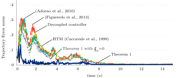
Figure 2: Tracking control error.

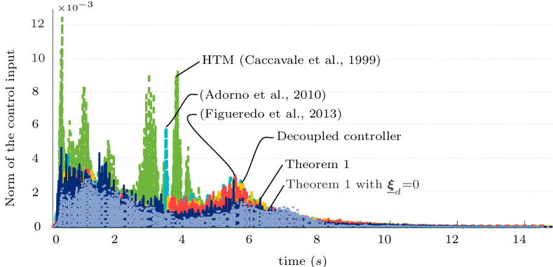
Figure 3: Trajectory tracking: norm of the control input.

5.3 $H_{\infty}$ robustness

To illustrate the performance of the proposed robust $H_{\infty}$ controller under different uncertainties and disturbances, a task was devised based on the motion of a mobile platform, a Pioneer P3-DX, which moved in triangle-wave fashion, alternating smoothly back and forth at fixed speed (respectively with period of $2.5\,s$ and $3.45\,s$). The end-effector had to track the non-fixed target with a constant relative pose. Since in this scenario the robot manipulator does not have knowledge of the mobile base velocity, the trajectory has an additional unknown twist, which is a disturbance that directly affects the relative pose.

Theorem 1 was used with different values of ${\gamma_{{}_{\mathcal{T}}}}$, while keeping ${\gamma_{{}_{\mathcal{O}}}}=2$ constant. Table 1 summarizes the numerically computed noise to error attenuation,

$${\gamma_{{}_{\mathcal{T}}}}_{\text{sim}} {=}\tfrac{\int_{0}^{T}\left\|\operatorname{\mathscr{T}\negmedspace}\left(\tilde{\underline{\boldsymbol{z}}}\left(t\right)\right)\right\|^{2}dt}{\int_{0}^{T}\left\|\boldsymbol{v}_{w}^{\prime}\left(t\right)\right\|^{2}+\left\|\boldsymbol{v}_{c}^{\prime}\left(t\right)\right\|^{2}dt}, \negthickspace{\gamma_{{}_{\mathcal{O}}}}_{\text{sim}}{=} \tfrac{\int_{0}^{T}\left\|\operatorname{\mathcal{\mathscr{O}}\negmedspace}\left(\tilde{\underline{\boldsymbol{z}}}\left(t\right)\right)\right\|^{2}dt}{\int_{0}^{T}\left\|\boldsymbol{v}_{w}\left(t\right)\right\|^{2}+\left\|\boldsymbol{v}_{c}\left(t\right)\right\|^{2}dt}.$$

As expected from the $H_{\infty}$ norm given by Definition 1, the noise to error attenuation remains below the prescribed thresholds, i.e., ${\gamma_{{}_{\mathcal{O}}}}_{\text{sim}}{\leq}{\gamma_{{}_{\mathcal{O}}}}$ and ${\gamma_{{}_{\mathcal{T}}}}_{\text{sim}}{\leq}{\gamma_{{}_{\mathcal{T}}}}$, for all ${\gamma_{{}_{\mathcal{O}}}}$, ${\gamma_{{}_{\mathcal{T}}}}$.

Table 1: Comparison between theoretical upper bound (${\gamma_{{}_{\mathcal{T}}}}$, ${\gamma_{{}_{\mathcal{O}}}}$) with the numerically calculated noise-to-error attenuation (${\gamma_{{}_{\mathcal{T}}}}_{\text{sim}}$, ${\gamma_{{}_{\mathcal{O}}}}_{\text{sim}}$).

${\gamma_{{}_{\mathcal{T}}}}$	$3.5$	$2.0$	$0.9$	$0.6$	$0.5$	$0.4$	$0.2$
${\gamma_{{}_{\mathcal{T}}}}_{\text{sim}}$	$1.914$	$1.235$	$0.736$	$0.528$	$0.404$	$0.326$	$0.167$
${\gamma_{{}_{\mathcal{O}}}}$	$2$	$2$	$2$	$2$	$2$	$2$	$2$
${\gamma_{{}_{\mathcal{O}}}}_{\text{sim}}$	$0.95$	$1.01$	$0.99$	$1.03$	$1.04$	$1.01$	$0.99$

The proposed controller, with ${\gamma_{{}_{\mathcal{T}}}}{=}0.4,\,{\gamma_{{}_{\mathcal{O}}}}{=}1$, was again compared to the dual-quaternion based controllers from Adorno et al. (2010) and Figueredo et al. (2013), and the HTM-based controller (Caccavale et al., 1999). To maintain fairness, all controllers were manually set to ensure similar control effort in terms of $\int_{0}^{T}\left\|\boldsymbol{u}\left(t\right)\right\|dt$. The numerically calculated noise-to-error attenuation from the simulations, presented in Table 2, shows that for the same control effort our controller outperforms the other ones in terms of disturbance attenuation.

Table 2: Numerically computed noise-to-error attenuation (${\gamma_{{}_{\mathcal{T}}}}_{\text{sim}}$, ${\gamma_{{}_{\mathcal{O}}}}_{\text{sim}}$) compared against theoretical values ${\gamma_{{}_{\mathcal{T}}}}{=}0.4$ and ${\gamma_{{}_{\mathcal{O}}}}{=}1.0$.

Theorem 1	Figueredo et al.	Adorno et al.	HTM
${\gamma_{{}_{\mathcal{T}}}}_{\text{sim}}{=}\boldsymbol{0.32}$	${\gamma_{{}_{\mathcal{T}}}}_{\text{sim}}{=}0.63$	${\gamma_{{}_{\mathcal{T}}}}_{\text{sim}}{=}0.61$	${\gamma_{{}_{\mathcal{T}}}}_{\text{sim}}{=}0.67$
${\gamma_{{}_{\mathcal{O}}}}_{\text{sim}}{=}\boldsymbol{0.65}$	${\gamma_{{}_{\mathcal{O}}}}_{\text{sim}}{=}0.86$	${\gamma_{{}_{\mathcal{O}}}}_{\text{sim}}{=}0.87$	${\gamma_{{}_{\mathcal{O}}}}_{\text{sim}}{=}0.78$

6 Experimental Results

This section presents results from the implementation on a real Meka Robotics A2 Arm, which is a highly compliant anthropomorphic $7$-joint manipulator and presents several unmodeled dynamic effects. We defined a trajectory over a helix curve in space with $10$ cm of both radius and axis length. Fig. 4 illustrates the trajectory with the aid of light-painting technique. We implemented the controller using C$++$ and the DQ Robotics toolbox (Adorno and Marinho, 2020) on ROS with a $8$ ms sampling period. For the experiment, the end-effector pose used in the control-loop was computed through the FKM.

The task trajectory was executed with different values for ${\gamma}={\gamma_{{}_{\mathcal{T}}}}={\gamma_{{}_{\mathcal{O}}}}$. Each experimental condition was then executed ten times for statistical significance (a total of $50$ trials). Results are summarized in Table 3 in terms of mean square error and standard deviation integrated along the trajectory. As expected, the $H_{\infty}$ controller is able to deal with disturbances originated, for instance, from the coupled nonlinear dynamics, measurement noise, parameter’s uncertainties, among others. Indeed, assuming similar disturbances conditions in all trials—which is reasonable as the experimental conditions were the same—and normalizing the results over the worst performance (i.e., the mean square error $\mathrm{MSE}_{\max}$ corresponding to ${\gamma}{=}\bar{\gamma}{\triangleq}1.86$), the average disturbance-to-error attenuation improvements ($\nicefrac{{\mathrm{MSE}_{\max}}}{{\mathrm{MSE}}}$) were almost inversely proportional to the decrease in ${\gamma}$. Fig. 4b shows the error along the trajectory for one execution of the robust controller for performance bounds ${\gamma}\in\{1.86,0.93,0.37\}$. As the theory predicts, setting smaller values for ${\gamma}$ yields a controlled system with better disturbance attenuation, which is manifested by smaller errors. In this case, since we did not directly measure the end-effector pose, the error is given with respect to the nominal value obtained through the FKM.

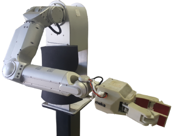
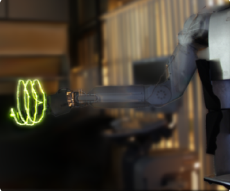
(a) Meka Robotics A2 Arm (left) and executed helicoidal trajectory with light-painting (right).

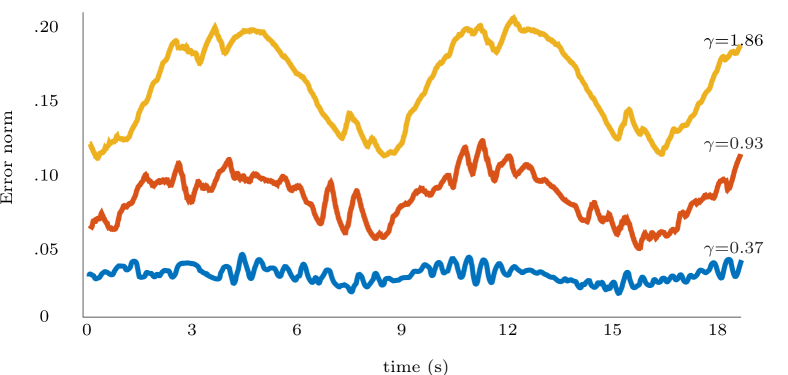
(b) Error trajectory for different values of prescribed noise-to-error upper bound $\gamma=\gamma_{\mathcal{T}}=\gamma_{\mathcal{O}}$ for one execution.

Figure 4: Experiments on the real robot manipulator.

Table 3: Average mean square error (MSE) and standard deviation (STD) under different performance conditions for the real experiment.

	$\bar{\gamma}{\triangleq}1.86$	$\frac{1}{2}\bar{\gamma}=0.93$	$\frac{1}{3}\bar{\gamma}=0.62$	$\frac{1}{4}\bar{\gamma}=0.47$	$\frac{1}{5}\bar{\gamma}=0.37$
$\mathrm{MSE}\pm\mathrm{STD}$	$\boldsymbol{3.118}\pm 0.015$	$1.662\pm 0.007$	$1.123\pm 0.011$	$0.829\pm 0.011$	$0.662\pm 0.005$
$\nicefrac{{\mathrm{MSE}_{\max}}}{{\mathrm{MSE}}}$	$1$	$1.87$	$2.78$	$3.76$	$4.71$

6.1 Practical Considerations

When implementing the controller (12) on a digital computer, instability issues may arise if the tracking bandwidth is too high compared to the inner joint-level control-loop bandwidth. Fortunately, modern manipulators have very fast joint controllers, often around 1 KHz, while the outer-loop often runs between 20–125 Hz. Also, considering the discrete-time joint dynamics given by $\Delta\boldsymbol{q}_{k+1}{=}a\Delta\boldsymbol{q}_{k}{+}bT\boldsymbol{u}$, where $a\in(-1,1)$, $b>0$, $\Delta\boldsymbol{q}_{k}=\boldsymbol{q}_{k}-\boldsymbol{q}_{k-1}$, and $T$ is the sampling time, Bjerkeng et al. (2014) show that the gain $\kappa=\kappa_{\mathcal{T}}=\mathcal{\kappa_{\mathcal{O}}}$ for a controller such as (12) should respect $\kappa<2(1+a)/bT$. Assuming $T=1\mathrm{ms}$ and a tuned controller (i.e., $a\approx 0$), one has $\kappa<2000/b$. Thus, $\kappa$ can still be very large without affecting the practical closed-loop stability.

7 Further Discussions and Conclusions

In this paper, we have exploited the geometrical significance of the dual quaternion algebra to derive an easy-to-implement closed-form $H_{\infty}$ task-space controller for the non-Euclidean space $\text{Spin}(3)\ltimes\mathbb{R}^{3}$ that describes the end-effector pose. Realistic simulations and experiments on a real robot were performed in different conditions and with different control strategies, which led to the following conclusions: a) compared to similar controllers with same convergence rate for regulation, the proposed controller requires less instantaneous control effort when no disturbances affect the system, and it has improved tracking performance; b) when there are disturbances, if all controllers are tuned to have similar control effort, the proposed controller ensures less set-point and tracking errors.

Lastly, our method works even when the end-effector pose is not directly measured because it can be estimated using the FKM. Although for most commercial robots the FKM provides sufficiently accurate end-effector poses, the nominal value may still differ from the real one due to several reasons. In that case, our strategy may be used to attenuate the influence of any disturbances over the end-effector trajectory, even if the FKM is not accurate enough. The residual error will then be bounded by the magnitude of the unknown transformation between the estimated and the actual end-effector pose.

Appendix A Derivative of the Lyapunov function

From (10), $\tilde{\underline{\boldsymbol{z}}}\triangleq 1-\tilde{\underline{\boldsymbol{x}}}=\tilde{\boldsymbol{z}}+\varepsilon\tilde{\boldsymbol{z}}^{\prime}$. By letting $\tilde{\underline{\boldsymbol{x}}}\triangleq\eta+\boldsymbol{\mu}+\varepsilon\left(\eta^{\prime}+\boldsymbol{\mu}^{\prime}\right)$, the positive definite functions $V_{1}$ and $V_{2}$ in the Lyapunov function (14) can be rewritten as

$$V_{1}(\tilde{\boldsymbol{z}}\left(t\right)) =\alpha_{1}\left\|\tilde{\boldsymbol{z}}(t)\right\|^{2}{=}\alpha_{1}\left(\left(1{-}\eta\right)^{2}+\left\|\boldsymbol{\mu}\right\|^{2}\right){=}2\alpha_{1}\left(1{-}\eta\right),$$

$$V_{2}(\tilde{\boldsymbol{z}}^{\prime}\left(t\right)) =\alpha_{2}\left\|\tilde{\boldsymbol{z}}^{\prime}(t)\right\|^{2}{=}\alpha_{2}\left(\eta^{\prime 2}+\left\|\boldsymbol{\mu}^{\prime}\right\|^{2}\right).$$

The derivative of (14) yields $\dot{V}_{1}(\tilde{\boldsymbol{z}}\left(t\right))+\dot{V}_{2}(\tilde{\boldsymbol{z}}^{\prime}\left(t\right))$ with

$$\dot{V}_{1}(\tilde{\boldsymbol{z}}\left(t\right)) {=}-2\alpha_{1}\dot{\eta},\,\,\text{and }\dot{V}_{2}(\tilde{\boldsymbol{z}}^{\prime}\left(t\right)){=}2\alpha_{2}\eta^{\prime}\dot{\eta}^{\prime}+2\alpha_{2}\langle\boldsymbol{\mu}^{\prime},\dot{\boldsymbol{\mu}}^{\prime}\rangle.$$

Using the closed-loop dynamics (13), we obtain

$$\dot{\eta} =-\tfrac{1}{2}\langle\boldsymbol{h}_{1},\boldsymbol{\mu}\rangle,\quad\quad\dot{\eta}^{\prime}=-\tfrac{1}{2}\left(\langle\boldsymbol{h}_{1},\boldsymbol{\mu}^{\prime}\rangle+\langle\boldsymbol{h}_{2},\boldsymbol{\mu}\rangle\right),$$

$$\dot{\boldsymbol{\mu}}^{\prime} =\tfrac{1}{2}\left(\eta^{\prime}\boldsymbol{h}_{1}+\eta\boldsymbol{h}_{2}+\boldsymbol{h}_{1}\times\boldsymbol{\mu}^{\prime}+\boldsymbol{h}_{2}\times\boldsymbol{\mu}\right),$$

where $\boldsymbol{h}_{1}=\kappa_{{\text{\tiny$\mathcal{O}$}}}\operatorname{\mathcal{\mathscr{O}}\negmedspace}\left(\tilde{\underline{\boldsymbol{z}}}\right)+\boldsymbol{v}_{w}+\boldsymbol{v}_{c}$ and $\boldsymbol{h}_{2}=-\kappa_{{\text{\tiny$\mathcal{T}$}}}\operatorname{\mathscr{T}\negmedspace}\left(\tilde{\underline{\boldsymbol{z}}}\right)+\boldsymbol{v}_{w}^{\prime}+\boldsymbol{v}_{c}^{\prime}.$ Hence,

$$\dot{V}_{1}(\tilde{\boldsymbol{z}}(t)) =\alpha_{1}\langle\boldsymbol{\mu},\boldsymbol{h}_{1}\rangle,$$ (21)

$$\dot{V}_{2}(\tilde{\boldsymbol{z}}^{\prime}(t)) =\alpha_{2}\langle\eta\boldsymbol{\mu}^{\prime}-\eta^{\prime}\boldsymbol{\mu}+\boldsymbol{\mu}\times\boldsymbol{\mu}^{\prime},\boldsymbol{h}_{2}\rangle.$$ (22)

To investigate the first condition from Definition 1, which regards exponential stability of (13) in the absence of disturbances $\underline{\boldsymbol{v}}_{w}$ and $\underline{\boldsymbol{v}}_{c}$, let us rewrite (21)-(22) as $\dot{V}(\tilde{\underline{\boldsymbol{z}}}\left(t\right))=\dot{V}_{1}(\tilde{\boldsymbol{z}}\left(t\right))+\dot{V}_{2}(\tilde{\boldsymbol{z}}^{\prime}\left(t\right))$ with

$$\dot{V}_{1}(\tilde{\boldsymbol{z}}\left(t\right)) =\alpha_{1}\langle\boldsymbol{\mu},\kappa_{{\text{\tiny$\mathcal{O}$}}}\operatorname{\mathcal{\mathscr{O}}\negmedspace}\left(\tilde{\underline{\boldsymbol{z}}}\right)\rangle,$$

$$\dot{V}_{2}(\tilde{\boldsymbol{z}}^{\prime}\left(t\right)) =-\alpha_{2}\langle\eta\boldsymbol{\mu}^{\prime}-\eta^{\prime}\boldsymbol{\mu}+\boldsymbol{\mu}\times\boldsymbol{\mu}^{\prime},\kappa_{{\text{\tiny$\mathcal{T}$}}}\operatorname{\mathscr{T}\negmedspace}\left(\tilde{\underline{\boldsymbol{z}}}\right)\rangle.$$

From (11) and considering the unit dual quaternion constraint $\eta\eta^{\prime}+\langle\boldsymbol{\mu},\boldsymbol{\mu}^{\prime}\rangle=0$ (Kussaba et al., 2017), we have $\operatorname{\mathscr{T}\negmedspace}\left(\tilde{\underline{\boldsymbol{z}}}\right)=2(\eta\boldsymbol{\mu}^{\prime}-\eta^{\prime}\boldsymbol{\mu}+\boldsymbol{\mu}\times\boldsymbol{\mu}^{\prime})$ and $\operatorname{\mathcal{\mathscr{O}}\negmedspace}\left(\tilde{\underline{\boldsymbol{z}}}\right)=-\boldsymbol{\mu}$; therefore,

$$\dot{V}_{1}(\tilde{\boldsymbol{z}}\left(t\right)) =-\alpha_{1}\kappa_{{\text{\tiny$\mathcal{O}$}}}\langle\boldsymbol{\mu},\boldsymbol{\mu}\rangle=-\alpha_{1}\kappa_{{\text{\tiny$\mathcal{O}$}}}\left\|\boldsymbol{\mu}\right\|^{2},$$

$$\begin{split}\dot{V}_{2}(\tilde{\boldsymbol{z}}^{\prime}\left(t\right))&=-2\alpha_{2}\kappa_{{\text{\tiny$\mathcal{T}$}}}\left(\eta^{2}\langle\boldsymbol{\mu}^{\prime},\boldsymbol{\mu}^{\prime}\rangle+\eta^{\prime 2}\langle\boldsymbol{\mu},\boldsymbol{\mu}\rangle-2\eta\eta^{\prime}\langle\boldsymbol{\mu},\boldsymbol{\mu}^{\prime}\rangle\right.\\ &\left.\hphantom{=-2\alpha_{2}\kappa_{{\text{\tiny$\mathcal{T}$}}}+}+\langle\boldsymbol{\mu},\boldsymbol{\mu}\rangle\langle\boldsymbol{\mu}^{\prime},\boldsymbol{\mu}^{\prime}\rangle-\langle\boldsymbol{\mu},\boldsymbol{\mu}^{\prime}\rangle^{2}\right).\end{split}$$

Notice the identity $\langle\boldsymbol{\mu}{\times}\boldsymbol{\mu}^{\prime},\boldsymbol{\mu}{\times}\boldsymbol{\mu}^{\prime}\rangle{=}\langle\boldsymbol{\mu},\boldsymbol{\mu}\rangle\langle\boldsymbol{\mu}^{\prime},\boldsymbol{\mu}^{\prime}\rangle{-}\langle\boldsymbol{\mu},\boldsymbol{\mu}^{\prime}\rangle^{2}$ in the last equality. Since $\langle\boldsymbol{\mu},\boldsymbol{\mu}^{\prime}\rangle=-\eta\eta^{\prime}$ and $\eta^{2}+\left\|\boldsymbol{\mu}\right\|^{2}=1$,

$$\dot{V}_{1}(\tilde{\boldsymbol{z}}\left(t\right)) {=}-\alpha_{1}\frac{\kappa_{{\text{\tiny$\mathcal{O}$}}}}{2}\left(\left\|\boldsymbol{\mu}\right\|^{2}{+}\left\|\boldsymbol{\mu}\right\|^{2}\right)=-\alpha_{1}\frac{\kappa_{{\text{\tiny$\mathcal{O}$}}}}{2}\left(1{-}\eta^{2}{+}\left\|\boldsymbol{\mu}\right\|^{2}\right),$$

$$\dot{V}_{2}(\tilde{\boldsymbol{z}}^{\prime}\left(t\right)) {=}{-}2\alpha_{2}\kappa_{{\text{\tiny$\mathcal{T}$}}}\Bigl{(}\negmedspace\eta^{2}\negmedspace\left\|\boldsymbol{\mu}^{\prime}\right\|^{2}{+}\eta^{\prime 2}\left\|\boldsymbol{\mu}\right\|^{2}{+}\eta^{2}\eta^{\prime 2}{+}\left(1{-}\eta^{2}\right)\negmedspace\left\|\boldsymbol{\mu}^{\prime}\right\|^{2}\negmedspace\Bigr{)}$$

$${=}-2\alpha_{2}\kappa_{{\text{\tiny$\mathcal{T}$}}}\left(\eta^{\prime 2}{+}\left\|\boldsymbol{\mu}^{\prime}\right\|^{2}\right){=}{-}2\alpha_{2}\kappa_{{\text{\tiny$\mathcal{T}$}}}\left\|\tilde{\boldsymbol{z}}^{\prime}(t)\right\|^{2}\negmedspace.\negthickspace$$ (23)

For $\eta{\in}[0,1],$ it is easy to see that $\left(1{-}\eta\right)^{2}\leq\left(1{-}\eta^{2}\right).$ Thus,

$$\dot{V}_{1}(\tilde{\boldsymbol{z}}\left(t\right))\leq-\alpha_{1}\frac{\kappa_{{\text{\tiny$\mathcal{O}$}}}}{2}\left(\left(1-\eta\right)^{2}+\left\|\boldsymbol{\mu}\right\|^{2}\right)=-\alpha_{1}\frac{\kappa_{{\text{\tiny$\mathcal{O}$}}}}{2}\left\|\tilde{\boldsymbol{z}}(t)\right\|^{2},$$ (24)

and, therefore,

$$\dot{V}(\tilde{\underline{\boldsymbol{z}}}\left(t\right)) \leq-\alpha_{1}\frac{\kappa_{{\text{\tiny$\mathcal{O}$}}}}{2}\left\|\tilde{\boldsymbol{z}}(t)\right\|^{2}-2\alpha_{2}\kappa_{{\text{\tiny$\mathcal{T}$}}}\left\|\tilde{\boldsymbol{z}}^{\prime}(t)\right\|^{2},$$

which in turn yields (15).

Remark 1.

To address the interval $\eta\in[-1,0]$ and prevent the problem of unwinding (Kussaba et al., 2017), one must assume $\tilde{\underline{\boldsymbol{z}}}=1+\tilde{\underline{\boldsymbol{x}}}$ instead of (10). Hence, without loss of generality, the exact same controller from Theorem 1 yields (15) with $\left\|\tilde{\boldsymbol{z}}(t)\right\|^{2}=\left(1{+}\eta\right)^{2}{+}\left\|\boldsymbol{\mu}\right\|^{2}$ where $\eta=-1$ is the equilibrium.

Now, if we explicitly regard the influence of $\underline{\boldsymbol{v}}_{w}$ and $\underline{\boldsymbol{v}}_{c}$, the Lyapunov derivative (21)-(22) yields

$$\dot{V}(\tilde{\underline{\boldsymbol{z}}}\left(t\right)) =-\alpha_{1}\langle\operatorname{\mathcal{\mathscr{O}}\negmedspace}\left(\tilde{\underline{\boldsymbol{z}}}\right),\kappa_{{\text{\tiny$\mathcal{O}$}}}\operatorname{\mathcal{\mathscr{O}}\negmedspace}\left(\tilde{\underline{\boldsymbol{z}}}\right){+}\boldsymbol{v}_{w}{+}\boldsymbol{v}_{c}\rangle$$

$$\qquad+\frac{\alpha_{2}}{2}\langle\operatorname{\mathscr{T}\negmedspace}\left(\tilde{\underline{\boldsymbol{z}}}\right),-\kappa_{{\text{\tiny$\mathcal{T}$}}}\operatorname{\mathscr{T}\negmedspace}\left(\tilde{\underline{\boldsymbol{z}}}\right)+\boldsymbol{v}_{w}^{\prime}{+}\boldsymbol{v}_{c}^{\prime}\rangle,$$ (25)

which is equivalent to (16).

Appendix B Decoupled controller

Given $\underline{\boldsymbol{x}}=\boldsymbol{r}+\left(1/2\right)\varepsilon\boldsymbol{p}\boldsymbol{r}$ and $\underline{\boldsymbol{x}}_{d}=\boldsymbol{r}_{d}+\left(1/2\right)\varepsilon\boldsymbol{p}_{d}\boldsymbol{r}_{d}$, the control input is

$$\dot{\boldsymbol{q}} \negmedspace=\negmedspace\boldsymbol{J}_{\mathrm{dec}}^{+}\kappa\negmedspace\left[\negmedspace\begin{array}[]{c}\operatorname{vec}_{3}\left(\boldsymbol{p}_{d}-\boldsymbol{p}\right)\\ \mathrm{vec}_{4}\left(1-\boldsymbol{r}^{*}\boldsymbol{r}_{d}\right)\end{array}\negmedspace\right]\negmedspace, \text{with }\boldsymbol{J}_{\mathrm{dec}} \negmedspace=\negmedspace\begin{bmatrix}\boldsymbol{J}_{p}\\ \boldsymbol{N}_{R_{4}}\end{bmatrix},$$

where $\mathrm{vec}_{4}\,:\,\mathcal{\mathbb{H}}\to\mathbb{R}^{4}$ is analogous to $\operatorname{vec}_{3}$ and the velocity satisfies $\operatorname{vec}_{3}\dot{\boldsymbol{p}}=\boldsymbol{J}_{p}\dot{\boldsymbol{q}}$. The matrix $\boldsymbol{N}_{R_{4}}$ corresponds to the four upper rows of $\boldsymbol{N}_{\!R_{8}}$, in which $\boldsymbol{N}_{\!R_{8}}=\smash{\overset{-}{\operatorname{\boldsymbol{H}}}\left(\underline{\boldsymbol{x}}_{d}\right)}\boldsymbol{C}_{8}\boldsymbol{J}_{\!R_{8}}$, with $\boldsymbol{C}_{8}=\mathrm{diag}\left(1,-1,-1,-1,1,-1,-1,-1\right)$, and $\boldsymbol{J}_{\!R_{8}}$ is the Jacobian matrix that satisfies $\mathrm{vec}_{8}\dot{\underline{\boldsymbol{x}}}=\boldsymbol{J}_{\!R_{8}}\dot{\boldsymbol{q}}$, where $\mathrm{vec}_{8}\,:\,\mathcal{H}\to\mathbb{R}^{8}$ is analogous to $\operatorname{vec}_{6}$.

References

- Abu-Khalaf et al. (2006) Abu-Khalaf, M., Huang, J., Lewis, F.L., 2006. Nonlinear / Constrained Feedback Control. Springer-Verlag, London.
- Adorno (2011) Adorno, B.V., 2011. Two-arm Manipulation: From Manipulators to Enhanced Human-Robot Collaboration. Ph.D. thesis. Laboratoire d’Informatique, de Robotique et de Microélectronique de Montpellier (LIRMM) - Université Montpellier 2. France.
- Adorno et al. (2015) Adorno, B.V., Bó, a.P.L., Fraisse, P., 2015. Kinematic modeling and control for human-robot cooperation considering different interaction roles. Robotica 33, 314–331.
- Adorno et al. (2010) Adorno, B.V., Fraisse, P., Druon, S., 2010. Dual position control strategies using the cooperative dual task-space framework, in: International Conference on Intelligent Robots and Systems (IROS), pp. 3955–3960.
- Adorno and Marinho (2020) Adorno, B.V., Marinho, M.M., 2020. DQ Robotics: a Library for Robot Modeling and Control Using Dual Quaternion Algebra. IEEE Robotics & Automation Magazine , 1–12.
- Aspragathos and Dimitros (1998) Aspragathos, N.A., Dimitros, J.K., 1998. A Comparative Study of Three Methods for Robot Kinematics. IEEE Transactions on Systems, Man, and Cybernetics, Part B: Cybernetics 28, 135–145.
- Bjerkeng et al. (2014) Bjerkeng, M., Falco, P., Natale, C., Pettersen, K.Y., 2014. Stability Analysis of a Hierarchical Architecture for Discrete-Time Sensor-Based Control of Robotic Systems. IEEE Trans. Robotics 30.
- Caccavale et al. (1999) Caccavale, F., Siciliano, B., Villani, L., 1999. The role of Euler parameters in robot control. Asian Journal of Control 1, 25–34.
- Figueredo et al. (2013) Figueredo, L., Adorno, B., Ishihara, J., Borges, G., 2013. Robust kinematic control of manipulator robots using dual quaternion representation, in: IEEE International Conference on Robotics and Automation (ICRA), pp. 1949–1955.
- Figueredo et al. (2014) Figueredo, L., Adorno, B., Ishihara, J., Borges, G., 2014. Switching strategy for flexible task execution using the cooperative dual task-space framework, in: Intelligent Robots and Systems (IROS 2014), 2014 IEEE/RSJ International Conference on, pp. 1703–1709.
- Han et al. (2008) Han, D.P., Wei, Q., Li, Z.X., 2008. Kinematic control of free rigid bodies using dual quaternions. Int. J. Autom. & Comp. 5, 319–324.
- Khalil (1996) Khalil, H., 1996. Nonlinear Systems. 2nd ed., Prentice-Hall.
- Kussaba et al. (2017) Kussaba, H.T., Figueredo, L.F.C., Ishihara, J.Y., Adorno, B.V., 2017. Hybrid kinematic control for rigid body pose stabilization using dual quaternions. Journal of the Franklin Institute 354.
- Marinho et al. (2019) Marinho, M.M., Adorno, B.V., Harada, K., Mitsuishi, M., 2019. Dynamic Active Constraints for Surgical Robots Using Vector-Field Inequalities. IEEE Transactions on Robotics 35, 1166–1185.
- Mas and Kitts (2017) Mas, I., Kitts, C., 2017. Quaternions and Dual Quaternions: Singularity-Free Multirobot Formation Control. Journal of Intelligent & Robotic Systems 87, 643–660.
- Selig (2005) Selig, J.M., 2005. Geometric fundamentals of robotics. 2nd ed., Springer-Verlag New York Inc.
- Simon (2006) Simon, D., 2006. Optimal State Estimation: Kalman, , and Nonlinear approaches. Wiley-Interscience.
- Wang and Yu (2013) Wang, X., Yu, C., 2013. Unit dual quaternion-based feedback linearization tracking problem for attitude and position dynamics. Systems & Control Letters 62, 225–233.
- Wang et al. (2012) Wang, X., Yu, C., Lin, Z., 2012. A Dual Quaternion Solution to Attitude and Position Control for Rigid-Body Coordination. IEEE Transactions on Robotics 28, 1162–1170.