Quantitative estimation of effective viscosity in quantum turbulence

Abstract

We study freely decaying quantum turbulence by performing high resolution numerical simulations of the Gross-Pitaevskii equation (GPE) in the Taylor-Green geometry. We use resolutions ranging from $1024^{3}$ to $4096^{3}$ grid points. The energy spectrum confirms the presence of both a Kolmogorov scaling range for scales larger than the intervortex scale $\ell$, and a second inertial range for scales smaller than $\ell$. Vortex line visualizations show the existence of substructures formed by a myriad of small-scale knotted vortices. Next, we study finite temperature effects in the decay of quantum turbulence by using the stochastic Ginzburg-Landau equation to generate thermal states, and then by evolving a combination of these thermal states with the Taylor-Green initial conditions using the GPE. We extract the mean free path out of these simulations by measuring the spectral broadening in the Bogoliubov dispersion relation obtained from spatio-temporal spectra, and use it to quantify the effective viscosity as a function of the temperature. Finally, in order to compare the decay of high temperature quantum and that of classical flows, and to further calibrate the estimations of viscosity from the mean free path in the GPE simulations, we perform low Reynolds number simulations of the Navier-Stokes equations.

I Introduction

Turbulence in quantum fluids provides an exciting yet challenging scenario to explore multi-scale and out of equilibrium dynamics. A turbulent state in superfluid ⁴He was first envisioned by Feynman as a random interacting tangle of quantum vortex lines Feynman (1955); Donnelly (1991). More recently, quantum turbulence has been realized and studied in experiments on a wide variety of superfluid systems and Bose-Einstein condensates (BECs) Barenghi et al. (2014), such as bosonic superfluid ⁴He Vinen and Niemela (2002), its fermionic counterpart ³He Tsepelin et al. (2017), and BECs in traps Henn et al. (2009). It must be emphasized that the study of quantum turbulence in laboratory experiments is a challenging task, which requires measurements at very low temperatures and usually in small system sizes; therefore, any experimental progress relies heavily on technical advancements. This is where numerical and theoretical studies become important: firstly, by providing explanations for the experimental observations; and secondly, by probing regimes which are yet not directly accessible in current experimental set-ups. However, these approaches have limitations of their own.

From the experimental, numerical, and theoretical studies, turbulent quantum fluids are known to display hydrodynamic behavior at the large scales, showcasing, for example, a Kolmogorov energy cascade Nore et al. (1997a); Maurer and Tabeling (1998). At smaller scales, the dynamics are dominated instead by nonlinear interactions of Kelvin waves L’vov and Nazarenko (2010). The crossover scale between these two regimes is determined by the mean intervortex length. Understanding how this picture is affected by finite temperature effects in the experiments is the matter of ongoing research. Currently there is no single theory which covers all the systems and is capable of predicting the known dynamic effects across all the involved length and time scales. Therefore, much progress relies on phenomenological models, which at times are better suited for one type of problem than for others. Three important classes of phenomenological models are: (i) the two-fluid models, (ii) the vortex filament model, and (iii) the Gross-Pitaevskii equation (GPE), sometimes also referred to as the nonlinear Schrödinger equation.

The phenomenological two-fluid model was proposed independently by L. Tisza and L. Landau. In this model, originally developed for superfluid helium, the fluid is regarded as a physically inseparable mixture of two components: the superfluid and the normal fluid. Many of the flow properties of superfluid helium at low velocities can be described within the framework of this model Landau and Lifshitz (2012). One of its great successes was the prediction of the propagation of second sound. However, it does not account for the presence of quantum vortices, a very important feature of quantum flows.

An extension of the two-fluid model is provided by the Hall-Vinen-Bekharevich-Khalatnikov model Hall and Vinen (1956); Bekarevich and Khalatnikov (1961). This model incorporates the effect of interactions between the quantized vortices and the normal fluid by including a mutual friction term. In this model the distinction between individual vortices is ignored, and only length scales larger than the mean separation between quantum vortices are considered. Therefore, it is an effective, coarse-grained model, which provides a good description of superfluid turbulence at low Mach numbers. The model has been used to study large scale flow properties and intermittency in direct numerical simulations (DNSs) of quantum turbulence Roche et al. (2009); Shukla et al. (2015); Biferale et al. (2018), and in reduced dynamical systems based on shell models Wacks and Barenghi (2011); Boué et al. (2013, 2015); Shukla and Pandit (2016).

The vortex filament model Schwarz (1985) overcomes some of the limitations of the two-fluid and the HVBK models by regarding the quantized vortices as filaments in three-dimensions (3D), and evolving them under the Biot-Savart law plus a mutual friction term mimicking the coupling between the normal and superfluid components. However, vortex reconnection is taken care of on an ad hoc basis. This model is relevant in situations in which the core size is negligible in comparison to the characteristic length scales in the hydrodynamic description of the flow, e.g., the mean inter-vortex separation $\ell$ or the radius of curvature of the vortex filaments $R$, and has been used to study quantum turbulence at finite temperatures Baggaley et al. (2012); Khomenko et al. (2015).

Finally, at zero or near-zero temperatures, and for weakly interacting bosons, the GPE provides a good hydrodynamical description of a quantum flow, that naturally includes quantum vortices as exact solutions which can reconnect without the need for any extra ad hoc assumptions Koplik and Levine (1993). The first 3D DNSs of decaying quantum turbulence, using the GPE as a model of a zero-temperature quantum fluid, were performed some $20$ years ago with linear resolutions up to $N=512$ grid points in each spatial direction, in the geometry of the Taylor-Green (TG) vortex flow Nore et al. (1997b, a). An important aspect of the above studies was to introduce a preparation method to generate initial data for vortex dynamics with minimal sound emission; also, for the diagnostics, the total conserved energy was decomposed into the incompressible kinetic energy and other energy components, each with their corresponding spectra. The main achievement of these works was showing that at the moment of maximum incompressible kinetic energy dissipation, the incompressible kinetic energy spectrum displays a power-law scaling which is compatible with Kolmogorov’s $k^{-5/3}$ scaling. This scaling was later confirmed in both experimental Maurer and Tabeling (1998) and in other numerical Kobayashi and Tsubota (2005) studies. The GPE has also been used to study the small-scale Kelvin wave cascade Clark di Leoni et al. (2015a); Villois et al. (2016), thus showing that both cascades can be captured by its dynamics. More recently, high resolution simulations resolving simultaneously the two inertial ranges (one for scales larger than the intervortex length, the other for smaller scales) were performed Clark di Leoni et al. (2017). This study also showed that at large scales the GPE can reproduce the dual cascade of energy and helicity observed in classical turbulence Brissaud et al. (1973).

However, a problem with the GPE is that finite temperature effects can be notoriously difficult to include Gardiner and Zoller (2000); Gardiner et al. (2002); Calzetta et al. (2007). One minimalistic approach, used in the present study, is to use the so-called classical field models Proukakis and Jackson (2008), by spectrally truncating the GPE Berloff et al. (2014). It is well known that the long time integration of the truncated system results in microcanonical equilibrium states that can capture a condensation transition Davis et al. (2001). This transition was later reproduced in Ref. Krstulovic and Brachet (2011a) using a grand-canonical method, where it was shown to be a standard second-order $\lambda$-transition. Moreover, dynamical counterflow effects on vortex motion, such as mutual friction and thermalization dynamics, were also shown to be correctly captured by this approach, and investigated in Refs. Krstulovic and Brachet (2011a, b). This scheme was also used to study the different regimes which appear during the relaxation dynamics of the turbulent two-dimensional (2D) GPE, where the complete thermalization states exhibit Berezinskii-Kosterlitz-Thouless transition in the microcanonical ensemble framework Shukla et al. (2016); Pandit et al. (2017); also, as in the case of 3D this was method was extended to compute the mutual friction coefficients in 2D Shukla et al. (2014).

Using this approach, finite temperature effects were recently studied in helical quantum turbulence Clark Di Leoni et al. (2018), where it was observed that close to the critical temperature the truncated system acts as a classical viscous flow, with the decay of the incompressible kinetic energy becoming exponential in time. From this observation, it was proposed that a quantitative estimation of the effective viscosity can be obtained by measuring the mean free path of the thermal excitations directly on the spatio-temporal spectrum of the flow as a function of the temperature, as this spectrum gives access to the spectrum of phonons in the system Clark di Leoni et al. (2015a). However, the calculation of the spatio-temporal spectrum is computationally intensive, and therefore, it is reasonable to perform it on a flow such as the TG vortex, that (as a result of its symmetries) maximizes the scale separation for given computational resources.

The purpose of the present paper is thus twofold. First, we want to extend the zero-temperature ($T=0$) TG vortex results at linear resolution $N=512$, obtained $20$ years ago, to the resolutions achievable with current computing resources. Second, we want to measure, at the highest possible spatial resolution, the spatio-temporal spectrum of the flow, in order to estimate the mean free path and its associated effective viscosity.

The rest of the paper is organized as follows. In Sec. II we present the details of the GPE model which we use, and of its numerical implementation. In particular, in Sec. II.1 we discuss the basic zero-temperature GPE theory and our diagnostics in terms of different energies and associated spectra. Section II.2 contains the details of our zero-temperature initial data preparation. Our methods of incorporating finite temperature effects are reviewed in Sec. II.3. We describe the numerical implementation of the problem in Sec. II.4, and in Sec. II.5 we discuss the choice of units. Section III contains our results. First, in Sec. III.1 we present our results for zero-temperature GPE dynamics with linear spatial resolutions up to $N=4096$. In Sec. III.2 we present the characterization of the finite-temperature GPE states, including the condensation transition. We give our results on the finite-temperature decaying GPE runs in Sec. III.3. In Sec. III.4 we compute and discuss the truncated GPE spatio-temporal correlation and spectra. We evaluate the mean-free path in Sec. III.5 and Sec. III.6 is devoted to the comparison of the finite-temperature freely decaying GPE runs with Navier-Stokes freely decaying runs. Finally, we present our conclusions in Sec. IV.

II Model, initial conditions, and numerical methods

II.1 Gross-Pitaevskii theory

The GPE is a partial differential equation for a complex field $\psi$ that describes the dynamics of a zero-temperature and dilute superfluid Bose-Einstein condensate. It reads

$$i\hbar\frac{\partial{\psi}}{\partial t}=-{\frac{\hbar^{2}}{2m}}\mbox{${\bf\nabla}^{2}$}\psi+{g}|\psi|^{2}\psi,$$ (1)

where $|\psi|^{2}$ is the number of particles per unit volume, $m$ is the mass of the bosons, $g=4\pi\tilde{a}\hbar^{2}/m$, and $\tilde{a}$ is the $s$-wave scattering length. This equation conserves the total energy $E$, the total number of particles $\mathcal{N}_{p}$, and the momentum ${\bf P}$, defined in a volume $V$ respectively as

$$E = \int_{V}d^{3}x\left({\frac{\hbar^{2}}{2m}}|\nabla\psi|^{2}+\frac{g}{2}|\psi|^{4}\right),$$ (2)

$$\mathcal{N}_{p} = \int_{V}|\psi|^{2}\,d^{3}x,$$ (3)

$${\bf P} = \int_{V}\frac{i\hbar}{2}\left(\psi{\bf\nabla}\overline{\psi}-\overline{\psi}{\bf\nabla}\psi\right)\,d^{3}x,$$ (4)

where the overline denotes the complex conjugate.

Equation (1) can be mapped into hydrodynamic equations of motion for a compressible irrotational fluid using the Madelung transformation given by

$$\psi({\bf x},t)=\sqrt{\frac{\rho({\bf x},t)}{m}}\exp{[i\frac{m}{\hbar}\phi({\bf x},t)]},$$ (5)

where $\rho({\bf x},t)$ is the fluid density, and $\phi({\bf x},t)$ is the velocity potential such that the fluid velocity is ${\bf v}={\bf\nabla}\phi$. The Madelung transformation is singular on the zeros of $\psi$. As two conditions are required in the singular points (both real and imaginary parts of $\psi$ must vanish), these singularities must take place on points in two-dimensions (2D) and on curves in 3D. The Onsager-Feynman quantum of velocity circulation around vortex lines with $\psi=0$ is given by $h/m$.

When Eq. (1) is linearized around a constant state $\psi=A_{0}$, one obtains the Bogoliubov dispersion relation

$$\omega_{B}(k)=\sqrt{\frac{gk^{2}|A_{0}|^{2}}{m}+\frac{\hbar^{2}k^{4}}{4m^{2}}}.$$ (6)

The sound velocity is thus given by $c=\sqrt{g|A_{0}|^{2}/m}$, with dispersive effects taking place for length scales smaller than the coherence length defined by

$$\xi=\sqrt{\hbar^{2}/(2gm|A_{\bf 0}|^{2})};$$ (7)

$\xi$ is also proportional to the radius of the vortex cores Nore et al. (1997b, a).

II.1.1 Energy decomposition and associated spectra

Following references Nore et al. (1997b, a), we define the total energy per unit volume as $e_{\rm tot}=(E-\mu\mathcal{N}_{p})/V-\mu^{2}/2g$, where $\mu$ is the chemical potential. Using the hydrodynamic fields, $e_{\rm tot}$ can we written as the sum of three components: the kinetic energy $e_{\rm kin}$, the internal energy $e_{\rm int}$, and the quantum energy $e_{\rm q}$ (all per unit volume), defined respectively as

$$e_{\rm kin} = \frac{1}{V}\int d^{3}x\frac{1}{2}(\sqrt{\rho}{\bf v})^{2},$$ (8)

$$e_{\rm int} = \frac{1}{V}\int d^{3}x\frac{g}{2m^{2}}\left(\rho-\rho_{0}\right)^{2},$$ (9)

$$e_{\rm q} = \frac{1}{V}\int d^{3}x\frac{\hbar^{2}}{2m^{2}}\left(\nabla\sqrt{\rho}\right)^{2},$$ (10)

where $\rho_{0}=m|A_{\bf 0}|^{2}$ is the mean density of the fluid. The kinetic energy ${e_{\rm kin}}$ can be further decomposed into a compressible component $e_{\rm kin}^{\rm c}$ and an incompressible component $e_{\rm kin}^{\rm i}$, by making use of the relation $\sqrt{\rho}{\bf v}=(\sqrt{\rho}{\bf v})^{\rm c}+(\sqrt{\rho}{\bf v})^{\rm i}$ with ${\bf\nabla}\cdot(\sqrt{\rho}{\bf v})^{\rm i}=0$ (see Nore et al. (1997b, a) for details).

Using Parseval’s theorem one can also construct corresponding energy spectra for each of these energies: e.g., the kinetic energy spectrum $e_{\rm kin}(k)$ is defined as

$$e_{\rm kin}(k)=\frac{1}{2}\int\left|\frac{1}{V}\int d^{3}re^{i{\bf r}\cdot{\bf k}}\sqrt{\rho}{\bf v}\right|^{2}k^{2}d\Omega_{k},$$ (11)

where $d\Omega_{k}$ is the solid angle element on the sphere in Fourier space.

II.1.2 Vortex line length estimation

Working in a similar fashion as with the energy, we can define the incompressible momentum power spectrum

$$P^{i}(k)=\frac{1}{2}\int\left|\frac{1}{V}\int d^{3}re^{i{\bf r}\cdot{\bf k}}(\rho{\bf v})^{i}\right|^{2}k^{2}d\Omega_{k}.$$ (12)

As was checked empirically in Refs. Nore et al. (1997b, a), the high wavenumber components of this spectrum can be approximated as the sum of the momentum of all the vortices present in the flow counted individually. This fact provides an easy way to estimate the total line length of the vortices in the flow. One simply has to calculate the total incompressible momentum omitting the first wavenumbers, and compare it to the momentum of a system where only one straight vortex line spanning the whole box length is present. As a result, the total vortex length $L_{V}$ is

$$\frac{L_{V}}{2\pi}=\frac{\int_{3}^{k_{\rm max}}P^{i}(k)dk}{\int_{3}^{k_{\rm max}}P^{i}_{\mathrm{single}}(k)dk},$$ (13)

where $k_{\rm max}$ is the maximum resolved wavenumber in the simulation, $P^{i}_{\mathrm{single}}(k)$ is the incompressible momentum power spectrum of a single vortex core (which can be calculated numerically by preparing the adequate initial conditions, or semi-analytically by using an axisymmetric solution of the GPE, see Nore et al. (1997b)), and the factor $2\pi$ is the length of the computational domain. The average intervortex distance, $\ell$, can finally be estimated from the total vortex length by looking at the vortex line density, $L_{V}/V$, in the following way

$$\ell^{-2}=\frac{L_{V}}{V}.$$ (14)

II.2 Zero-temperature initial data preparation

The TG initial condition $\psi_{\rm TG}$ is such that its nodal lines correspond to vortex lines of the so-called Taylor-Green flow. In dimensionless units, the TG velocity flow ${\bf u}_{\rm TG}$ is defined as

$$u^{\rm TG}_{x}(x,y,z) = \sin(x)\cos(y)\cos(z),$$

$$u^{\rm TG}_{y}(x,y,z) = -\cos(x)\sin(y)\cos(z),$$

$$u^{\rm TG}_{z}(x,y,z) = 0.$$ (15)

II.2.1 Taylor-Green symmetries

The symmetries of the TG velocity field are rotational symmetries of angle $\pi$ around the axes $x=z=\pi/2$, $y=z=\pi/2$, and $x=y=\pi/2$, and mirror symmetries with respect to the planes $x=0$ & $\pi$, $y=0$ & $\pi$, and $z=0$ & $\pi$. The TG velocity field is parallel to these planes, that form the sides of an impermeable box which confines the flow. It is demonstrated in Ref. Brachet et al. (1983) that when using ${\bf u}_{\rm TG}$ as initial data for the Navier-Stokes equations, these symmetries are preserved by the dynamics, and that its solutions admit the following Fourier expansion:

$$u_{x} = \sum_{m=0}^{\infty}\sum_{n=0}^{\infty}\sum_{p=0}^{\infty}\hat{u}_{x}(m,n,p)\sin mx\cos ny\cos pz,$$

$$u_{y} = \sum_{m=0}^{\infty}\sum_{n=0}^{\infty}\sum_{p=0}^{\infty}\hat{u}_{y}(m,n,p)\cos mx\sin ny\cos pz,$$

$$u_{z} = \sum_{m=0}^{\infty}\sum_{n=0}^{\infty}\sum_{p=0}^{\infty}\hat{u}_{z}(m,n,p)\cos mx\cos ny\sin pz,$$ (16)

where $\hat{\bf u}(m,n,p)$ vanishes unless $m,n,p$ are either all even or all odd integers. The expansion coefficients should also satisfy:

$$\hat{u}_{x}(m,n,p) = (-1)^{r+1}\hat{u}_{y}(n,m,p),$$

$$\hat{u}_{z}(m,n,p) = (-1)^{r+1}\hat{u}_{z}(n,m,p),$$ (17)

where $r=1$ when $m,n,p$ are all even, and $r=2$ when $m,n,p$ are all odd. These come from the fact that the TG flow has a rotational symmetry of angle $\pi/2$ around the axis $x=y=\pi/2$.

	Resolution
$\xi k_{\rm max}$	$N=128$	$N=256$	$N=512$
$1.5$	–	$e_{\lambda}=4.17$	–
		$T_{\lambda}=3.25$
$2.5$	$e_{\lambda}=10.64$	$e_{\lambda}=10.13$	$e_{\lambda}=9.12$
	$T_{\lambda}=9.5$	$T_{\lambda}=9.25$	$T_{\lambda}=8.75$
$4$	–	$e_{\lambda}=24.12$	–
		$T_{\lambda}=23.5$

Table 1: Transition energy $e_{\lambda}=E_{\lambda}/V$, and temperature $T_{\lambda}$ in the phase transition, for sets of runs at different spatial linear resolution $N$, and with different values of $\xi k_{\rm max}$. Values of the energies and temperatures are in units of $MU^{2}L^{-3}$.

These symmetries can be extended to flows described by the GPE in Eq. (1). It is easy to show that the expressions in Eq. (16) applied to $\rho v_{j}$, with $v_{j}=\partial_{j}\phi$, (see Eq. 5), correspond to the following decomposition for the complex scalar $\psi(x,y,z,t)$ as a solution of the GPE

$$\psi=\sum_{m=0}^{\infty}\sum_{n=0}^{\infty}\sum_{p=0}^{\infty}\hat{\psi}(m,n,p)\cos mx\cos ny\cos pz,$$ (18)

with $\hat{\psi}(m,n,p)=0$ unless $m,n,p$ are either all even or all odd integers. The additional conditions then become

$$\hat{\psi}(m,n,p)=(-1)^{r+1}\hat{\psi}(n,m,p)$$ (19)

with the same convention as above. Implementing these relations in a numerical code yields savings of a factor $64$ in computational time and memory size when compared to the general Fourier expansion.

II.2.2 Taylor-Green initial data

In order to create the initial condition $\psi_{\rm TG}$ with zeros along vortex lines of ${\bf u}_{\rm TG}$, we make use of the Clebsch representation of the velocity field Nore et al. (1997b, a). The Clebsch potentials

$$\lambda(x,y,z) = \cos x\sqrt{2\;|\cos z|},$$

$$\mu(x,y,z) = \cos y\sqrt{2\;|\cos z|}\;{\mbox{sgn}}(\cos z),$$ (20)

(where sgn is the sign function) generate the TG flow in Eq. (15), in the sense that $\nabla\times{\bf u}_{\rm TG}=\nabla\lambda\times\nabla\mu$. Also, note that a zero in the $(\lambda,\mu)$ plane corresponds to a vortex line of ${\bf u}_{\rm TG}$ (see Nore et al. (1997b, a) for details).

Defining the 2D complex field $\psi_{e}$ with a simple zero at the origin of the ($\lambda,\mu$) plane,

$$\psi_{e}(\lambda,\mu)=(\lambda+i\mu)\frac{\tanh(\sqrt{\lambda^{2}+\mu^{2}}/\sqrt{2}\xi)}{\sqrt{\lambda^{2}+\mu^{2}}},$$ (21)

we obtain a three dimensional field (as a function of $x$, $y$, and $z$) with one nodal line. We can further define

$$\psi_{4}(\lambda,\mu) = \psi_{e}(\lambda-\frac{1}{\sqrt{2}},\mu)\psi_{e}(\lambda,\mu-\frac{1}{\sqrt{2}}),$$ (22)

$$\times \psi_{e}(\lambda+\frac{1}{\sqrt{2}},\mu)\psi_{e}(\lambda,\mu+\frac{1}{\sqrt{2}}),$$

which contains four nodal lines. In order to match the circulation of ${\bf u}_{\rm TG}$, we finally define a field which will be used below as initial condition for an equation for data preparation as

$$\psi_{\rm ARGLE}(x,y,z)=\psi_{4}(\lambda(x,y,z),\mu(x,y,z))^{[\gamma_{d}/4]},$$ (23)

where the ratio of the total circulation to the elementary defect’s circulation is $\gamma_{d}=(2/\pi)\,\hbar/(2m)$ with $\hbar/(2m)=c\xi/\sqrt{2}$. Thus, initially each vortex line corresponds to a multiple zero line.

The final step in the initial data preparation method consists in running to convergence the Advective Real Ginzburg-Landau Equation (ARGLE):

$$\frac{\partial{\psi}}{\partial t}=\frac{\hbar}{2m}\mbox{${\bf\nabla}^{2}$}\psi+\mu\psi-\frac{g}{\hbar}|\psi|^{2}\psi-i{\bf u}_{\rm TG}\cdot\nabla\psi-\frac{|{\bf u}_{\rm TG}|^{2}}{2\hbar/m}\psi,$$ (24)

with the initial condition $\psi_{\rm ARGLE}$. The ARGLE evolution corresponds to the imaginary time propagation of the GPE with a local Galilean transformation by the velocity field ${\bf u}_{\rm TG}$. Under ARGLE dynamics the multiple zero lines in $\psi_{\rm ARGLE}$ will spontaneously split into single zero lines, and the system will finally converge to initial conditions for the GPE, compatible with the TG flow, and with minimal sound emission. We denote the resulting converged state as $\psi_{\rm TG}$.

$T/T_{\lambda}$	$e_{\textrm{tot}}[MU^{2}/L^{3}]$	$n_{0}$
$0$	$0.129$	$1$
$0.11$	$0.95$	$0.92$
$0.22$	$1.94$	$0.86$
$0.33$	$2.96$	$0.75$
$0.44$	$4.02$	$0.65$
$0.55$	$5.14$	$0.55$

Table 2: Variation of the total energy $e_{\textrm{tot}}$ and of the condensed fraction $n_{0}$ in the thermal runs with $N=1024$ and $\xi k_{\rm max}=2.5$ (for these parameters $T_{\lambda}=8.58$, in units of $MU^{2}/L^{3}$).

II.3 A finite temperature model

One of the different possible ways to include finite temperature effects on the condensate dynamics is by imposing an ultra-violet cutoff on the GPE. This amounts to performing a Galerkin truncation operation on the GPE in Fourier space with a projection operator $\mathcal{P}_{\rm G}$ defined as

$$\mathcal{P}_{\rm G}[\hat{\psi}({\bf k})]=\Theta(k_{\rm max}-|\bf{k}|)\hat{\psi}(\bf k),$$ (25)

where $\hat{\psi}$ is the spatial Fourier transform of $\psi$, $k_{\rm max}$ is a suitably chosen ultraviolet cutoff (which, in practice, will be the same as the maximum resolved wavenumber in the simulations), and $\Theta$ is the Heaviside function. The resulting Galerkin truncated GPE (TGPE) is

$$i\hbar\frac{\partial{\psi}}{\partial t}=\mathcal{P}_{\rm G}\left[-{\frac{\hbar^{2}}{2m}}\mbox{${\bf\nabla}^{2}$}\psi+{g}\mathcal{P}_{\rm G}\left[|\psi|^{2}\right]\psi\right].$$ (26)

The TGPE in Eq. (26) exactly conserves energy and mass; moreover, if we correctly de-alias it by using the $2/3-$dealiasing rule Gottlieb and Orszag (1977), with $k_{\rm max}=2/3\times N/2$ (in dimensionless units), it also conserves momentum. We refer to Ref. Krstulovic and Brachet (2011a) for an explicit demonstration of the latter. The Galerkin truncation operation also preserves the Hamiltonian structure with the truncated Hamiltonian of the system given by

$$H=\int d^{3}x\left[{\frac{\hbar^{2}}{2m}}|\nabla\psi|^{2}+\frac{g}{2}\left(\mathcal{P}_{\rm G}|\psi|^{2}\right)^{2}\right].$$ (27)

The grand canonical equilibrium states are given by the following stationary probability distribution

$$\mathbb{P}_{\rm st}[\psi]=\frac{1}{\mathcal{Z}}e^{-\beta[H-\mu\mathcal{N}_{p}]},$$ (28)

where $\mathcal{Z}$ is the grand partition function, $\beta=1/(k_{\rm B}T)$ is the inverse temperature, and $k_{\rm B}$ is the Boltzmann constant. However, these states are difficult to compute as the Hamiltonians in Eqs. (2) or (27) are not quadratic, and the resulting statistical distribution is non-Gaussian. Nevertheless, it is possible to construct a stochastic process that converges to a stationary solution with equilibrium distribution given by Eq. (28). This process is defined by a Langevin equation consisting of a stochastic Ginzburg-Landau equation (SGLE) that explicitly reads in physical space

$$\hbar\frac{\partial{\psi}}{\partial t} = \mathcal{P}_{\rm G}\left[{\frac{\hbar^{2}}{2m}}\mbox{${\bf\nabla}^{2}$}\psi+{\mu}\psi-{g}\mathcal{P}_{\rm G}\left[|\psi|^{2}\right]\psi\right]$$ (29)

$$\hskip 42.67912pt+\sqrt{\frac{2\hbar}{V\beta}}\mathcal{P}_{\rm G}\left[\zeta({\bf x},t)\right],$$

where the Gaussian white noise $\zeta({\bf x},t)$ obeys

$$\langle\zeta({\bf x},t)\overline{\zeta}({\bf x^{\prime}},t^{\prime})\rangle=\delta(t-t^{\prime})\delta({\bf x}-{\bf x^{\prime}}).$$ (30)

We refer to Ref. Krstulovic and Brachet (2011a) for more details on the proof of the equivalence of this stationary probability distribution to the grand canonical equilibrium state.

If one wants to control the number of particles $\mathcal{N}_{p}$ instead of the chemical potential $\mu$, then one must supplement the SGLE with an ad-hoc equation for the chemical potential

$$\frac{{\rm d}{\mu}}{{\rm dt}}=-\frac{\nu_{N}}{V}(\mathcal{N}_{p}-\mathcal{N}_{p}^{*}),$$ (31)

where $\mathcal{N}_{p}^{*}$ controls the mean number of particles and $\nu_{N}$ governs the rate at which SGLE equilibrates.

We will call the thermal states generated by the SGLE $\psi_{\mathrm{th}}$. These states can be used in the TGPE to compute their dynamical properties. Moreover, we can combine these thermal states with an initial condition for a large-scale flow to simulate quantum turbulence at finite temperature. For the TG flow, the combined initial state in this case reads:

$$\psi=\psi_{\mathrm{TG}}\times\psi_{\mathrm{th}}.$$ (32)

In the present study, we perform several DNSs of the SGLE in Eq. (29)) and of the TGPE in Eq. (26). For numerical purposes we rewrite the SGLE (omitting the Galerkin projector $\mathcal{P}_{\rm G}$) as

$$\frac{\partial{\psi}}{\partial t} = \alpha_{0}\mbox{${\bf\nabla}^{2}$}\psi+\Omega_{0}\psi-\beta_{0}|\psi|^{2}\psi+\sqrt{\frac{k_{B}T}{\alpha_{0}}}\zeta,$$

where $\alpha_{0}$, $\Omega_{0}$, and $\beta_{0}$ are parameters. We can express physically relevant quantities, such as the coherence length $\xi$ and the velocity of sound $c$, in terms of these new parameters. These are related by

$$\xi=\sqrt{\alpha_{0}/\Omega_{0}\,},\hskip 14.22636ptc=\sqrt{2\alpha_{0}\beta_{0}\rho_{0}},$$ (33)

with $\rho_{0}=\Omega_{0}/\beta_{0}$. In all the DNS runs presented below we set the density at $T=0$ to $\rho_{0}=1$ (in dimensionless units as described below). In order to keep the value of intensive variables constant in the thermodynamic limit, at constant volume $V$ and for $k_{\rm max}\to\infty$, the inverse temperature is expressed as $\beta=1/(k_{\rm modes}T)$, where $k_{\rm modes}=V/\mathcal{N}_{m}$ with $\mathcal{N}_{m}$ the number of Fourier modes in the system. With these definitions the temperature $T$ has units of energy per volume, and $4\pi\alpha_{0}$ is the quantum of circulation.

II.4 Numerical implementation

The code, TYGRS (TaYlor-GReen Symmetric), is a pseudo-spectral code that enforces the symmetries of the TG vortex in 3D for the GPE, the Navier-Stokes equations, and the magnetohydrodynamic equations within periodic cubes of length $2\pi$ (in dimensionless units). As a result of the symmetries discussed in Sec. II.2.1, the Fourier-transformed fields are non-zero only for wave vectors $(k_{x},k_{y},k_{z})=(m,n,p)$ with jointly even or jointly odd components. Time integration of only these Fourier modes is performed using a fourth-order Runge-Kutta method.

Pseudo-spectral codes are known to be optimal on periodic domains Gottlieb and Orszag (1977). However, they require global spectral transforms, and thus are hard to implement in distributed memory environments, a crucial limitation until domain decomposition techniques (DDTs) arose Calvin (1996); Dmitruk et al. (2001) that allowed computation of serial Fast Fourier Transforms (FFTs) in different directions in space (local in memory) after performing transpositions. However, distributed parallelization using the Message Passing Interface (MPI) in pseudo-spectral codes is limited in the number of processors that can be used, unless more transpositions are done per FFT (thus increasing communication time). To overcome this limitation, the hybrid (MPI-OpenMP) parallelization scheme we have implemented in TYGRS builds upon a general purpose one-dimensional (slab-based) DDT that is effective for parallel scaling using MPI alone Gómez et al. (2005), extended with OpenMP to obtain an (in practice) 2D DDT without the need of extra communication Mininni et al. (2011). In this scheme, each MPI task creates multiple threads using OpenMP which operate over a fraction of the available data. This method has been extended in TYGRS to the sine/cosine with even/odd wavenumber FFTs needed to implement the symmetries of TG flows, using loop-level OpenMP directives and multi-threaded FFTs. The method was shown to scale with high parallel efficiency to over 100,000 CPU cores Mininni et al. (2011).

The runs were performed on the IDRIS BlueGene/P machine. At resolution $N=4096$ we used $512$ MPI processes, each process spawning $4$ OpenMP threads, needing a total of $2048$ CPU cores per simulation.

II.5 Units

In the following, all quantities are expressed in terms of a unit length $L$, a unit speed $U$, and a unit mass $M$. These are related to the simulation length $L^{\prime}$, the characteristic speed $U^{\prime}$, and the actual mass $M^{\prime}$ in the following way

$$L =\frac{L^{\prime}}{2\pi},$$ (34)

$$U =\frac{U^{\prime}}{2},$$ (35)

$$M =\frac{M^{\prime}}{(2\pi)^{3}}.$$ (36)

With these choices the simulation box is $2\pi L$ long (in each spatial direction), the speed of sound $c$ is $2U$, and the mean density $\rho_{0}$ is equal to $1\,M/L^{3}$. The factors in Eqs. (34) to (36) result from the dimensionless scheme used in the simulations (done in a periodic box of dimensionless side $2\pi$).

In some of the simulations we present next, the healing length $\xi$ is such that $\xi k_{\max}=1.5$, or $\xi k_{\max}=2.5$, with a few cases with $\xi k_{\max}=4$ (each case is appropriately indicated in the text). As a result, in the simulation with the largest spatial resolution in this work with $\xi k_{\max}=2.5$, the healing length is $\xi\approx 0.0018L^{\prime}$. While the resolution in this simulation is state-of-the-art, the scale separation is not sufficient to be able to compare with superfluid ⁴He experiments, where the characteristic system size is $L^{\prime}\approx 10^{-2}$ m, the speed of sound is $c^{\prime}\approx 230$ m/s, the fluid density is $\approx 125$ kg/m³ (thus $M^{\prime}\approx 1.25\times 10^{-4}$ kg), and the healing length is $\xi^{\prime}\approx 10^{-8}\,\textrm{m}\approx 10^{-6}L^{\prime}$ Barenghi et al. (2014). On the other hand, scale separation in BEC experiments of quantum turbulence, where $L^{\prime}\approx 10^{-4}$ m, $c^{\prime}\approx 2\times 10^{-3}$ m/s, and $\xi\approx 5\times 10^{-7}\,\textrm{m}\approx 0.005L^{\prime}$ White et al. (2014); Tsatsos et al. (2016), is within our reach.

Except when explicitly noted, temperatures will be expressed in terms of the transition temperature $T_{\lambda}$. Finally, note that the intensity of non-linear interactions is controlled by the inverse of $\xi k_{\rm max}$ Krstulovic and Brachet (2011a). Indeed, for $\xi k_{\rm max}$ very large, most of the excitations correspond to free particles. More details on how units can be handled in DNSs of the GPE and SGLE can be found in Nore et al. (1997b); Krstulovic and Brachet (2011b, a); Clark Di Leoni et al. (2018).

III Results

We start this section by discussing the temporal evolution of the TG flow at zero temperature, using a resolution of $4096^{3}$ collocation points as well as simulations at lower resolution. We then perform a series of temperature scans to study the decay of the TG initial conditions at finite temperature. Finally, by computing the spatio-temporal spectra of these flows, we provide an estimation of the effective viscosity in flows evolved under the TGPE.

III.1 High resolution GPE runs at $T=0$

The TG initial data obtained following Eqs. (22)-(24) was first produced with $\xi k_{\rm max}=2.5$ and with linear spatial resolutions of $N=1024$, $2048$ and $4096$ grid points. The time evolution of the energies defined in Eqs. (8), (9), and (10) under the GPE dynamics are shown in Figs. 1(a) and 1(b) for the simulations with $N=2048$ and $N=4096$, respectively. In all cases, the total energy was conserved within a $2\%$ error. The incompressible kinetic energy per unit volume $e_{\rm kin}^{i}$ remains approximately constant until $t\approx 4\,L/U$, and afterwards it starts decaying as the other energy components increase to keep the total energy fixed. This indicates a transfer of energy from $e_{\rm kin}^{i}$ to the other energy components as turbulence develops (most conspicuously at late times for the $N=2048$ run, to the compressible component $e_{\rm kin}^{c}$). The vortex line length $L_{V}$, as defined in Eq. (13), is shown in Fig. 1(c) for all three simulations. At around $t\approx 8\,L/U$, $L_{V}$ peaks, and thus the maximum of incompressible kinetic energy dissipation is reached.

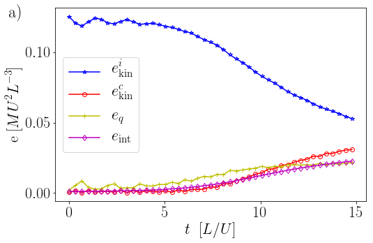
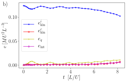
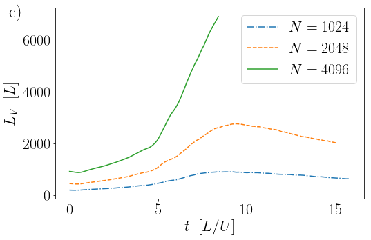
Figure 1: (Color online) Time evolution of the different energy components at zero temperature in (a) a 3D simulation with $N=2048$ grid points in each spatial direction, and (b) with $N=4096$ grid points in each direction. Both DNSs have $\xi k_{\rm max}=2.5$. (c) Time evolution of the total vortex line length $L$ in simulations at different spatial resolutions.

In Fig. 2(a) we show the incompressible kinetic energy spectra of the $N=4096$ simulation at different times, while in Fig. 2(b) we present the same spectra at $t=8\,L/U$ for the $N=1024$, $N=2046$, and $N=4096$ simulations. Round markers indicate the mean intervortex wavenumber $k_{\ell}=2\pi/\ell$, and the dashed lines indicate $k^{-5/3}$ power laws as a reference. On the one hand, at wavenumbers smaller than $k_{\ell}$, strong hydrodynamic turbulence is known to be the principal mechanism to transfer energy towards smaller scales. A Kolmogorov-like spectrum can thus be expected in this range of scales. On other hand, at wavenumbers larger than $k_{\ell}$, energy is expected to be carried towards even smaller scales by the Kelvin wave cascade L’vov and Nazarenko (2010). This cascade, predicted with weak-wave turbulence theory, also leads to a $k^{-5/3}$ scaling but with a different origin from the one of Kolmogorov. Note that the Kelvin wave cascade has been studied using the GPE before Krstulovic (2012), and it has been observed in GPE turbulence using spatio-temporal analysis Clark di Leoni et al. (2015a) and by direct measurement of vortex line excitations Villois et al. (2016). Also, the Kolmogorov and Kelvin wave cascades transfer the energy towards smaller scales at different rates. It is thus expected that energy should accumulate near the wavenumber $k_{\ell}$, resulting in a bottleneck in the spectrum L’vov et al. (2007). We indeed observe the emergence of a bottleneck in the vicinity of this wavenumber, although not as pronounced as the thermalization scaling $\sim k^{2}$. This difference might be due to the fact that the present simulations are freely decaying, and have no force acting to sustain turbulence. The existence of two simultaneous inertial ranges separated by a bottleneck was also observed before in high resolution simulations using different initial conditions Clark di Leoni et al. (2017), but was not visible in the $N=512$ DNS of a TG flow in Nore et al. (1997b) possibly as a result of the limited spatial resolution in that study. To further illustrate these ranges, and the scale separation involved, in Fig. 2(c) and (d) we show the incompressible kinetic energy spectra compensated by Kolmogorov scaling $\sim k^{-5/3}$.

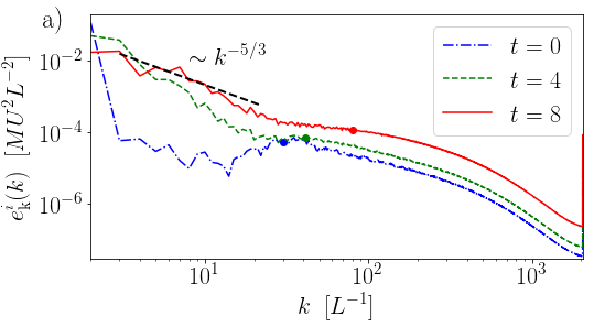
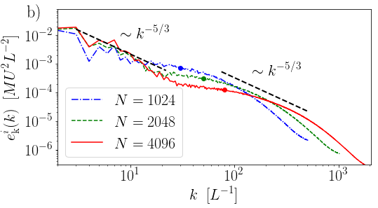
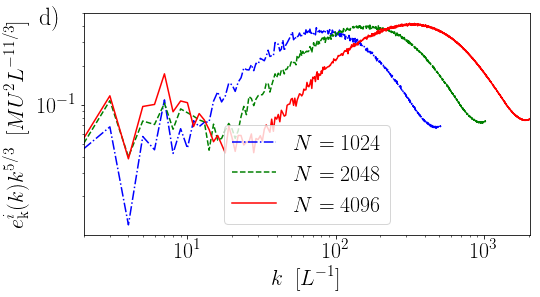
Figure 2: (Color online) a) Incompressible kinetic energy spectra $e^{i}_{\rm kin}(k)$ at zero temperature, at different times for the $N=4096$ simulation. b) Spectra at $t=8$ for three DNSs at different spatial resolution. In both panels, the circular marks indicate the mean intervortex wavenumber at the corresponding time, or for the corresponding spatial resolution. Power laws $\sim k^{-5/3}$ are shown as a reference, for scales larger and smaller than the intervortex scale. Note the emergence of a second intertial range, after a bottleneck, for scales smaler than the intervortex scale. (c) and (d) show the spectra from panel (a) and (b), but compensated by Kolmogorov scaling.

Visualizations of the vortex lines in the $N=4096$ run close to the time of maximum energy dissipation are shown in Fig. 3. The intricate vortex line tangle in the entire computational domain (for the TG impermeable box) is shown first. The large-scale flow shows inhomogeneous regions with high density of vortices and quiet regions with low density. Details into the central regions with high density of vortices (and large shear) are also shown. It should be noted that the tangle of vortices results from many reconnections taking place after $t\approx 4\,L/U$. Comparing these $N=4096$ results with those obtained $20$ years ago at resolution $N=512$ and presented in Fig. 18 of Ref. Nore et al. (1997b), we can note the presence of substructures made by a myriad of small-scale and knotted and linked vortices that were not apparent at the lower resolution.

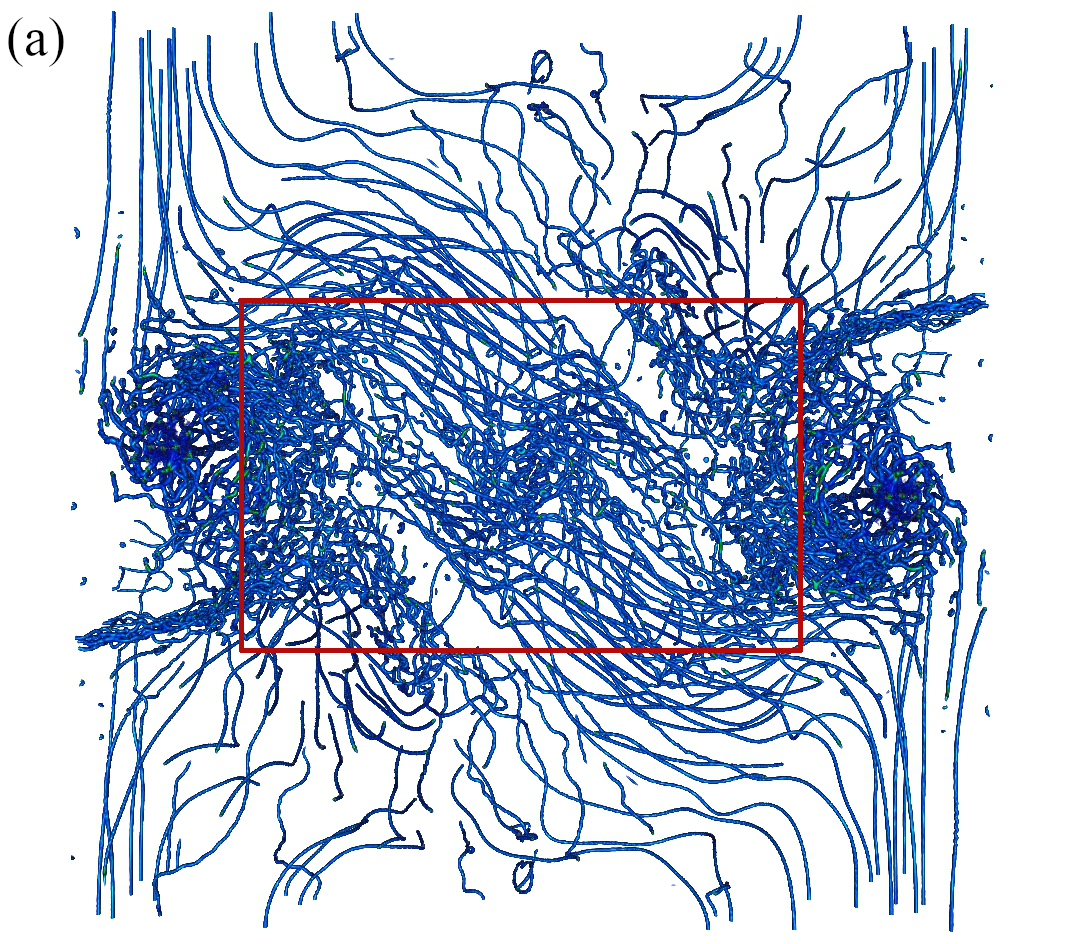
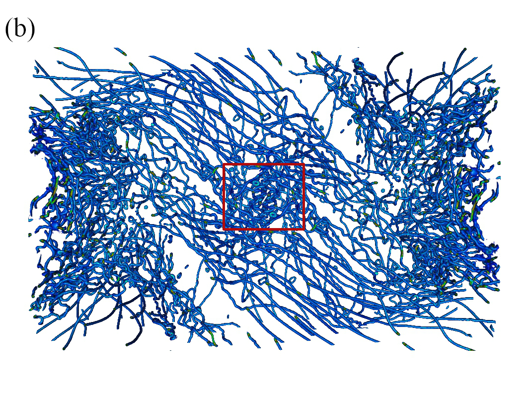
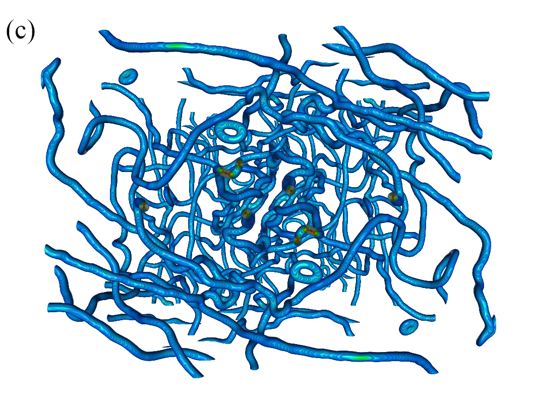
Figure 3: (Color online) Three-dimensional renderings of vortex lines at the onset of the decay in the $4096^{4}$ GPE run. (a) The full impermeable box. The (red) box indicates the region shown in panel (b), which shows a zoom into a region of the domain with large shear of the vortex lines. Again, the (red) box in this panel indicates the region zoomed into in panel (c). Note in the latter panel the tangle of vortices, the many links between vortices, and the helical deformations of individual vortices along the vortex line. Visualizations were prepared using the software VAPOR Clyne et al. (2007).

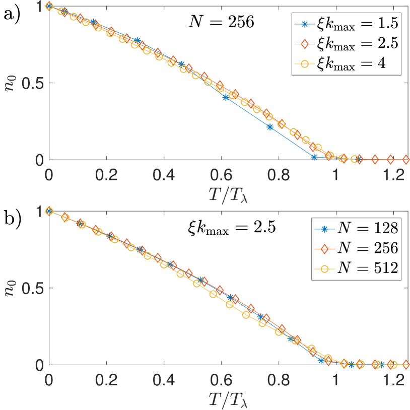
Figure 4: (Color online) (a) Condensed fraction as a function of $T/T_{\lambda}$ at linear resolution $N=256$ and for different values of $\xi k_{\rm max}$. (b) Condensed fraction as a function of $T/T_{\lambda}$ at $\xi k_{\rm max}=2.5$ and for different linear resolutions $N$. The condensed fraction is computed using Eq. (37) with $k_{c}=2$ for simulations with $N=128$, and with $k_{c}=4$ for all the other numerical simulations.

III.2 SGLE temperature scans

We now study only thermal states, in order to determine the condensation temperature $T_{\lambda}$ in our system with symmetries. We thus performed a series of SGLE temperature scans, with various values for the linear resolution $N$ and $\xi k_{\rm max}$, as indicated in Table 1. Each box in the table indicates the transition energy and temperature obtained, for a fixed value of $N$ and $\xi k_{\rm max}$, by performing 12 to 24 simulations in each set varying the temperature. Boxes without data correspond to cases not explored.

It is well known that the TGPE can capture the condensation transition Proukakis and Jackson (2008); Davis et al. (2001); Krstulovic and Brachet (2011a). The order parameter of this phase transition is the condensed fraction, which is usually defined as the fraction of atoms that are in the ground state. In terms of Fourier modes, it is given by $|\hat{\psi}({\bf k}=0)|^{2}/\mathcal{N}_{p}$. However, for the TG flow the symmetries cancel exactly the energy (and mass density) of some Fourier modes, decreasing the availability of Fourier modes at low wavenumbers, and thus affecting the dynamics of the condensed fraction. As a result, we define the condensed fraction as

$$n_{0}=\frac{1}{\mathcal{N}_{p}}\int_{{k=0}}^{k_{c}}|\widehat{\psi}_{\bf k}|^{2}k^{2}d\Omega_{k},$$ (37)

where $k_{c}$ is a small wave-number (either 2 or 4, in dimensionless units, depending on the spatial resolution $N$).

The condensed fraction as a function of the temperature is displayed in Fig. 4(a) for fixed spatial resolution $N$ and different values of $\xi k_{\rm max}$, and in Fig. 4(b) for fixed $\xi k_{\rm max}$ and different values of $N$. Note the transition in all cases at $T=T_{\lambda}$. The corresponding values of the transition temperatures $T_{\lambda}$ and energies $e_{\lambda}$ are given in Table 1.

The behavior of the different energy components as the temperature is varied, at fixed linear resolution of $N=256$ and for different values of $\xi k_{\rm max}$, is shown in Fig. 5. Note that for fixed $\xi k_{\rm max}$, $e_{\rm q}$ increases in all cases with $T$ up to $T_{\lambda}$, as also do $e_{\rm int}$ and $e_{\rm kin}^{i}$, while $e_{\rm kin}^{c}$ displays a maximum at intermediate temperatures. As expected, increasing the value of $\xi k_{\rm max}$ decreases the non-linear interactions, that can be quantified by the relative value of $e_{\rm int}(t)$.

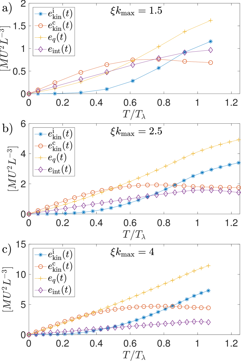
Figure 5: (Color online) Energy components as a function of the temperature, for different values of $\xi k_{\rm max}$, and for fixed linear spatial resolution ($N=256$). (a) Temperature scan with $\xi k_{\rm max}=1.5$, (b) same with $\xi k_{\rm max}=2.5$, and (c) same with $\xi k_{\rm max}=4$.

Comparing these TG symmetric results with those obtained for a general periodic geometry as given in Fig. 2 of Ref. Krstulovic and Brachet (2011a), it can be seen that the overall properties of the condensation transition are nor significantly affected by the nature of the geometry imposed by the symmetries at the largest scales. As a result, we now consider the combination of the thermal states with the TG flow.

III.3 Thermal equilibria combined with the TG flow

To study finite temperature effects in the TG flow, we prepared several high resolution thermal states (up to $T=0.55\,T_{\lambda}$) at linear resolution of $N=1024$, and with $\xi k_{\rm max}=2.5$ (see Table 2 for more details on the energy and condensed fraction in these states as $T$ is varied). We then combined these thermal states with the TG initial data prepared following Eqs. (22)-(24).

In Figs. 6(a)-(d) we show the GPE temporal evolution of the energy components $e^{i}_{\rm kin}$, $e^{c}_{\rm kin}$, $e_{\rm q}$, and $e_{\rm int}$ at four different temperatures ($T=0,\,0.11\,T_{\lambda},0.33\,T_{\lambda}$, and $0.55\,T_{\lambda}$). Similar to the case of high resolution runs at $N=2048$ and $4096$, the incompressible kinetic energy $e^{i}_{\rm kin}$ at $T=0$ shown in Fig. 6(a) stays roughly constant till $t\approx 5\,L/U$, followed by a large decay of approximately $30\%$ of its initial value in a similar interval of time (up to $t\approx 10\,L/U$); thereafter, its decay slows down. During the initial phase of the dynamical evolution of the TG flow, the decrease in the incompressible kinetic energy is accompanied by an increase in the other energy components, with $e_{\rm int}$ gaining the maximum share until $t\approx 10\,L/U$, after which it saturates. At the later stages, the compressible kinetic energy $e^{c}_{\rm kin}$ is the dominant component, with the internal energy having magnitude similar to $e_{\rm q}$ for the rest of the duration of the run.

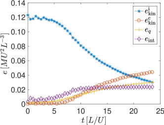
Figure 6: (Color online) Time evolution of the energy components in the TGPE runs with linear spatial resolution $N=1024$ and $\xi k_{\rm max}=2.5$ at four different temperatures: (a) $T=0\,T_{\lambda}$, (b) $0.11\,T_{\lambda}$, (c) $0.33\,T_{\lambda}$, and (d) $0.55\,T_{\lambda}$.

At higher temperatures, the plots of the different energy components in Figs. 6(c)-(d) show that $e^{c}_{\rm kin}$, $e_{\rm q}$, and $e_{\rm int}$ start with higher values when compared to the $T=0$ case, because of finite temperature effects included via the thermal states, and in agreement with the discussion in Sec. III.2 (see Fig. 5). In particular, in the runs with $T=0.33T_{\lambda}$ and with $0.55T_{\lambda}$, the incompressible kinetic energy has the lowest share of the total energy, while the compressible component is the dominant form of the energy (although at $T=0.55\,T_{\lambda}$, $e_{\rm q}$ also becomes comparable to $e^{c}_{\rm kin}$).

In spite of these differences at $t=0$ and at very early times, in all the cases presented in Fig. 6 we observe at later times a qualitatively similar decrease in $e^{i}_{\rm kin}$ as the TG flow evolves. For a better comparison, we plot the time evolution of $e^{i}_{\rm kin}$ at five different temperatures in Fig. 7(a). We note once again that besides the initial adaptation period which lasts roughly until $t\approx 1\,L/U$, the $e^{i}_{\rm kin}$ energy component decreases very slowly during the time interval $t\approx 2\,L/U$ to $4\,L/U$, wherein $e^{i}_{\rm kin}$ at $T=0$ remains roughly constant. After this time interval the decay of $e^{i}_{\rm kin}$ is faster. This behavior is still better captured by computing the decay rate $-de^{i}_{\rm kin}/dt$, a quantity frequently studied in freely decaying classical fluid turbulence. In Fig. 7(b) we show the temporal evolution of $-de^{i}_{\rm kin}/dt$ for different temperatures. If we discard the initial adaptation period, at least the low temperature curves (up to $T=0.44\,T_{\lambda}$) exhibit a peak at $t\approx 8\,L/U$, and the peak value decreases, along with an accompanying flattening, as we increase the temperature. At $T=0.55\,T_{\lambda}$, $-de^{i}_{\rm kin}/dt$ fluctuates around the value $5\times 10^{-3}MU^{3}L^{-4}$; however, because of the presence of strong fluctuations (and the lack of enough statistics), we are unable to make more precise statements for higher temperatures. Note that given these fluctuations, to identify trends while varying temperature, we use a filtering technique to smooth out the curves (not shown). It is also interesting to note that at around $t\approx 8\,L/U$ (when the peak in $-de^{i}_{\rm kin}/dt$ is observed), the vortex line length $L_{V}$ is maximum in the $T=0$ runs, see Sec. III.1 and Fig. 1(c).

Figure 7: (Color online) Time evolution of: (a) The incompressible kinetic energy $e^{i}_{\rm kin}$, and of (b) the incompressible kinetic energy dissipation rate $-de^{i}_{\rm kin}/dt$, at six different temperatures in TGPE runs with linear spatial resolution $N=1024$ and $\xi k_{max}=2.5$.

To better understand how the thermal fluctuations act across the different length scales during the evolution of the TG flow towards the turbulent state, in Fig. 8(a)-(d) we show the incompressible and compressible kinetic energy spectra for the $T=0$ case, and for three different temperatures ($T=0.11\,T_{\lambda}$, $0.33\,T_{\lambda}$, and $0.55\,T_{\lambda}$), at a time at which we observe a range of wavenumbers in the spectrum compatible with self-similar scaling (i.e., with a possible inertial range). For $T=0$, shown in Fig. 8(a), we observe that $e^{i}_{\rm kin}(k)\sim k^{-5/3}$ (at $t=6\,L/U$) roughly over a decade at small wavenumbers, followed by a bottleneck around $k\approx 20\,L^{-1}$, and an exponential decrease for even larger wavenumbers. The amplitude of the spectrum of compressible energy is amost negligible in this case and at this instant of time. For the runs at larger temperatures, shown in Figs. 8(b)-(d), we continue to observe a range of wavenumbers compatible with $e^{i}_{\rm kin}(k)\sim k^{-5/3}$ scaling (for small wavenumbers), but now at high wavenumbers we see an accumulation of energy and the begining of a thermalized region approaching $\sim k^{2}$ scaling, indicating small scale fluctuations become more energetic as we increase the temperature. At the same time, the amplitude of the compressible energy spectrum increases with increasing $T$, with $e^{c}_{\rm kin}(k)\sim k^{2}$ at highwave numbers as it is expected for a thermal state. In particular, for $T=0.55\,T_{\lambda}$ in Fig. 8(d), $e^{i}_{\rm kin}(k)$ does not show anymore a significant range with Kolmogorov scaling. This can be understood as the crossover region at which the range of wavenumbers compatible with an inertial range finishes, at $k\approx 20L^{-1}$ in the $T=0$ case, is strongly modified in this high temperature run by the thermal bath, which now affects and extends to smaller wave numbers, thereby reducing the inertial range.

Finally, to illustrate the time evolution of the spectra, we show in Fig. 9 the incompressible and compressible kinetic energy spectra in two runs at $T=0$ and at $T=0.33\,T_{\lambda}$, at different instants in time. The development in time of an inertial range at intermediate wavenumbers can be seen in all cases in $e^{i}_{\textrm{kin}}(k)$ (Kolmogorov scaling is indicated in Fig. 9 as a reference, as well as the thermalization scaling $\sim k^{2}$ for the spectrum of $e^{c}_{\textrm{kin}}$). A more detailed time evolution of these spectra can also be seen in the videos M1 ($T=0$) and M2 ($T>0$) in the supplemental material SMa .

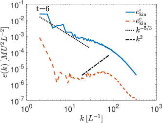
Figure 8: (Color online) Kinetic energy spectra $e^{i}_{\rm kin}(k)$ and $e^{c}_{\rm kin}(k)$ for four different temperatures: (a) $T=0\,T_{\lambda}$, (b) $0.11\,T_{\lambda}$, (c) $0.33\,T_{\lambda}$, and (d) $0.55\,T_{\lambda}$, from TGPE runs with linear spatial resolution $N=1024$ and $\xi k_{\rm max}=2.5$. Videos M1 ($T=0$) and M2 ($T>0$), see Supplemental Material SMa , show the time evolution of the compensated incompressible kinetic energy spectra at different temperatures.

Figure 9: (Color online) Temporal evolution of the kinetic energy spectra: (a) Incompressible component $e^{i}_{\rm kin}(k)$ at $T=0$; (b) incompressible component $e^{i}_{\rm kin}(k)$, and (c) compressible component $e^{c}_{\rm kin}(k)$, for the TGPE run at $T=0.33\,T_{\lambda}$ with linear spatial resolution $N=1024$ and $\xi k_{\rm max}=2.5$.

III.4 TGPE spatio-temporal spectra in thermal equilibrium

We now compute the spatio-temporal spectra (STS) of the thermal equilibria, that will be later used to estimate the mean-free path and the effective viscosity. To this end, some of the SGLE equilibria of Table 1 were used as initial data for GPE runs (with the same values of $N$ and $\xi k_{\rm max}$), and integrated in time.

The STS provides the power spectrum of a given quantity as a function of the wavenumber and of the frequency Clark di Leoni et al. (2014); Clark di Leoni et al. (2015b, a). To compute this spectrum, quantities of interest must be stored with high time cadence, so a Fourier transform in time and space can be computed resolving the relevant high frequencies involved in the problem. The result is a spectrum that shows the amplitude of the excitations as a function of $k$ and $\omega$, and that can be used to extract the amplitude of waves in a disordered state, as wave excitations should accumulate near the theoretical dispersion relation in $k-\omega$ space. In the following we consider the spatio-temporal power spectrum of $\psi$, which is the STS of mass fluctuations.

The STS for runs with $N=256^{3}$ and $\xi k_{\rm max}=1.5$, and for different temperatures, is shown in Fig. 10. At very low temperature ($T=0.05T_{\lambda}$) the non-linear interaction is very weak, leading to exacts resonances in the periodic domain. The only modes excited are those satisfying the Bogolioubov dispersion relation given by Eq. (6) (indicated as a reference by the dashed line), and modes with $\omega=0$ which correspond to the condensate. As the temperature increases, non-linear interactions become important and the dispersion relation broadens, as can be seen, e.g., for $T=0.31T_{\lambda}$. Also note that as the temperature is increased, the condensate (which in this figure appears as a straight horizontal bright line) is shifted to higher frequencies, as it takes place at energies $\hbar\omega=\mu$. The excitation of sound waves around the Bogoliubov dispersion relation keeps broadening for larger and larger temperatures up to $T_{\lambda}$, which is expected as the broadening should be the strongest close to the transition. For temperatures much larger than $T_{\lambda}$ the dispersion relation is given by free particles, and we expect to recover the standard 4-wave interaction. Also, note that for $T=1.08T_{\lambda}$ the condensate disappears. Figure 11 displays the same STS for runs with $\xi k_{\rm max}=2.5$. Although the qualitative behavior is the same, note that at a fixed temperature the spectral broadening is smaller, consistent with the fact that for large $\xi k_{\rm max}$ the non-linear interaction is expected to be weaker.

Based on these results, for a fixed $k$ we define the spectral broadening $\Delta\omega(k)$ as the width for which the accumulation of spectral power around the dispersion relation goes to half of its maximum amplitude. Note that $\Delta\omega(k)$ is associated with the inverse of the time of non-linearly interacting waves. The values of $\Delta\omega(k)$ extracted from the STS for different temperatures and values of $\xi k_{\rm max}$, as a function of $k$, can be seen in Fig. 12. Note that: (1) For fixed temperature, $\Delta\omega(k)$ increases with $k$, reaching its maximum value for $k\sim 1/\xi$, and then growing slowly or remaining approximately constant. (2) For fixed $k$, $\Delta\omega(k)$ increases with temperature, reaching its maximum value close to $T_{\lambda}$. And finally, (3) the role of the parameter $\xi k_{\rm max}$ controlling the strength of non-linear interactions between waves is confirmed by the values of $\Delta\omega(k)$, as the amplitude of this quantity is significantly reduced for increasing $\xi k_{\rm max}$.

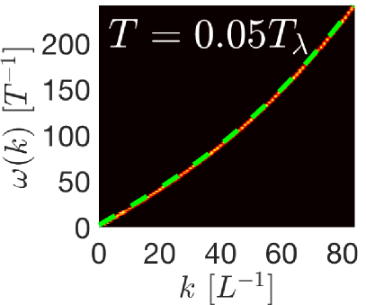
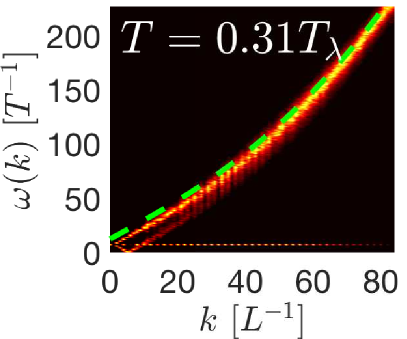
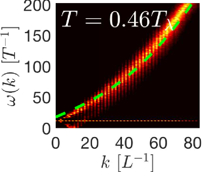
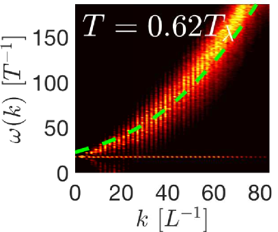
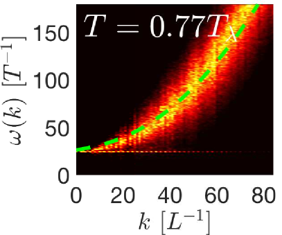
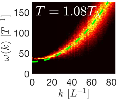
Figure 10: (Color online) Spatio-temporal spectra with $\xi k_{\rm max}=1.5$ and $N=256^{3}$, for different temperatures as indicated in each panel. The (green) dashed line indicates the theoretical Bogoliubov dispersion relation. Bright (red to yellow) areas indicate modes with large excitation.

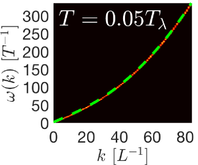
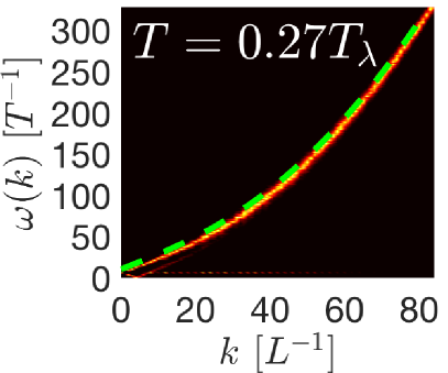
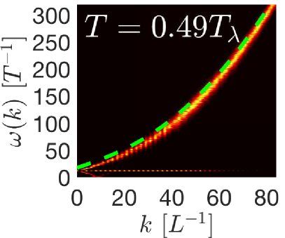
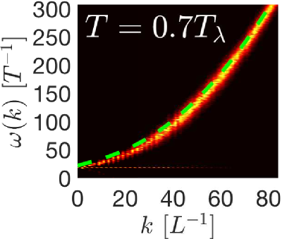
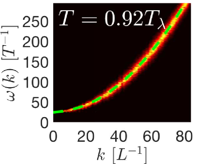
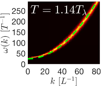
Figure 11: (Color online) Spatio-temporal spectra with $\xi k_{\rm max}=2.5$ and $N=256^{3}$, for different temperatures as indicated in each figure. The (green) dashed line indicates the theoretical Bogoliubov dispersion relation. Bright (red to yellow) areas indicate modes with large excitation.

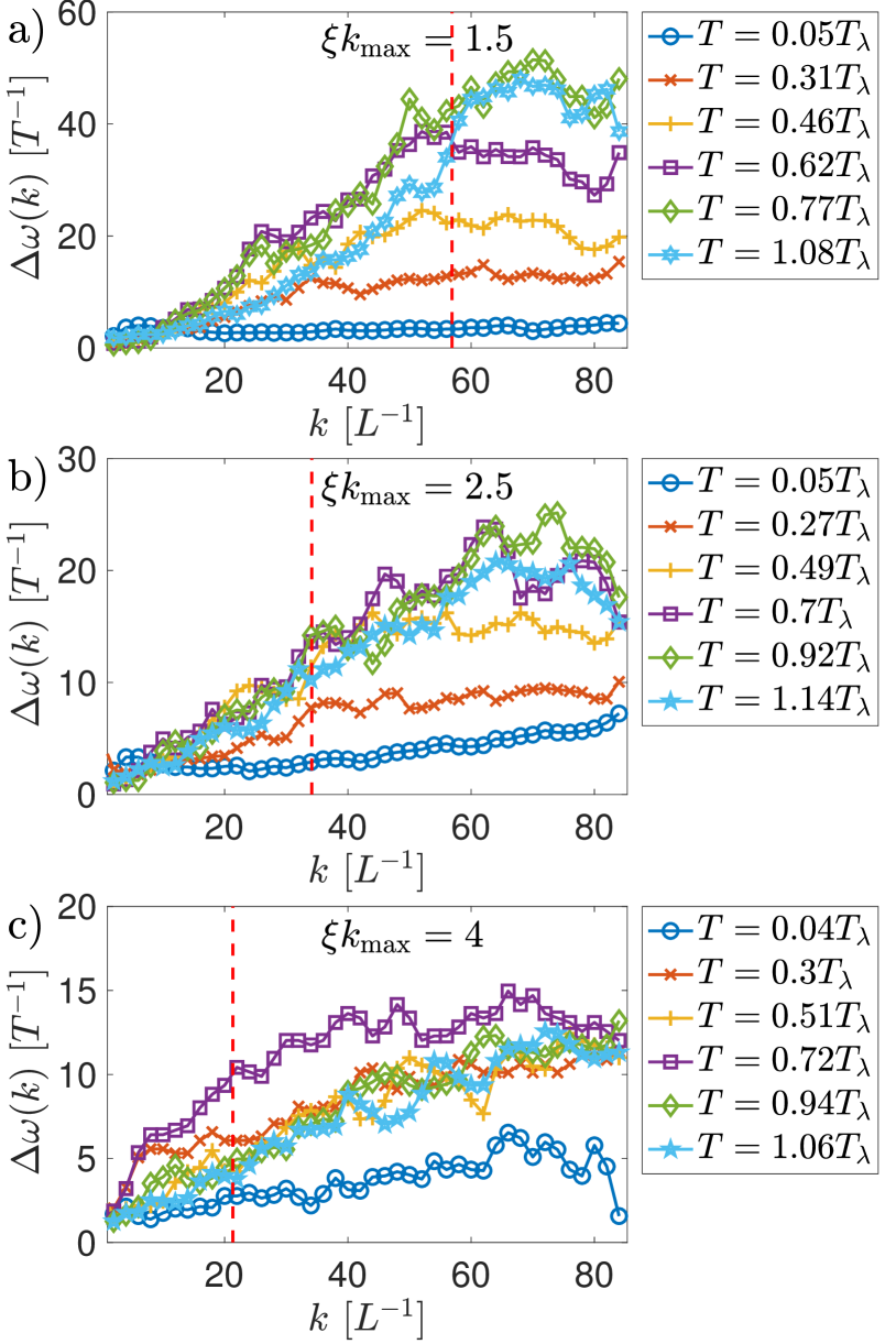
Figure 12: (Color online) Spectral broadening $\Delta\omega(k)$ of the dispersion relation, for different temperatures and values of $\xi k_{\rm max}$. The vertical dashed lines indicate the value of $1/\xi$ in each case: (a) as a function of $k$ for different temperatures and for $\xi k_{\rm max}=1.5$, (b) same for $\xi k_{\rm max}=2.5$, and (c) same for $\xi k_{\rm max}=4$.

III.5 Mean free path and effective viscosity

We turn now to estimate the mean free path and the effective viscosity for TGPE flows. As already mentioned, the time of non-linear wave interactions is associated to the inverse of $\Delta\omega$; during a time proportional to this quantity, waves travel without being scattered by other waves Nazarenko (2011). As a result, the mean free path can be constructed as

$$\lambda(k,T)\sim\frac{1}{\Delta\omega(k,T)}\frac{d\omega_{B}}{dk}.$$ (38)

In Fig. 13 we show the mean-free path of the simulations at different values of temperatures and $\xi k_{\rm max}$. The dispersion relation at different temperatures was directly measured from the STS in Fig. 11. For wavenumbers larger than $k\approx 1/\xi$, $\lambda(k,T)$ seems to saturate (or to fluctuate around a mean value for a range of wavenumbers larger than $1/\xi$) in many cases. We can then define a mean-free path at each temperature by taking $\lambda(T)=\lambda(k\approx k_{\max},T)$. The resulting plot of $\lambda(T)$ is shown in Fig. 14(a) for different values of $\xi k_{\rm max}$. As expected, it increases when $T$ goes to zero. Larger values of $\xi k_{\rm max}$ reduce the non-linear interactions and thus increase the mean-free path.

From the mean free path, we can estimate the effective viscosity by writing

$$\nu_{\rm eff}(T)\sim\lambda(T)\left.\frac{d\omega_{B}}{dk}\right|_{k\approx k_{\max}}=\frac{\left(\left.\frac{d\omega_{B}}{dk}\right|_{k\approx k_{\max}}\right)^{2}}{\Delta\omega(k\approx k_{\max},T)};$$ (39)

note that we evaluate $\Delta\omega(T)$ and $d\omega_{B}/dk$ at $k=80\approx k_{\max}$. In Fig. 14(b) we show $\nu_{\rm eff}(T)$ normalized by the quantum of circulation $4\pi\alpha=4\pi c\xi\sqrt{2}$. For temperatures above $0.5T_{\lambda}$, both $\lambda$ and $\nu_{\rm eff}$ are relatively constant. For the runs with $\xi k_{\rm max}=2.5$ we have

$$\lambda(T) \sim 10\xi,$$ (40)

$$\nu_{\rm eff}(T) \sim 50\alpha=50c\xi/\sqrt{2}.$$ (41)

Equation (41) gives a physical estimation of the scaling of the effective viscosity in terms of the sound velocity $c$ and of the healing length $\xi$. In the simulations, using $c=2U$ and $\xi=2.5/k_{\max}=2.5\times 3L/N$, the effective viscosity then becomes

$$\nu_{\rm eff}(T)\sim L\,U\frac{500}{N},$$ (42)

where $U$ and $L$ are the unit velocity and length, and $N$ is the linear spatial resolution. In dimensionless units, with $U=L=1$, the Reynolds number can then be estimated as

$$\mathrm{Re}^{\textrm{(TG)}}=\frac{C}{\nu_{\rm eff}}=\frac{CN}{500},$$ (43)

where $C$ is a prefactor of order unity (as $\nu_{\rm eff}$ is an effective transport coefficient, we can only ascertain its value from the mean free path up to a multiplicative constant).

The definition of the Reynolds number as $1/\nu_{\rm eff}$ is the usual definition in simulations of the Taylor-Green flow Brachet et al. (1983). As in the next section (Sec. III.6) we will compare GPE runs with simulations of the Navier-Stokes equations at low Reynolds numbers, it will be convenient to also use a definition of this number based on the dynamic r.m.s. flow velocity

$$U_{0}=\sqrt{2E}$$ (44)

and the flow correlation length

$$L_{0}=2\pi\,\frac{\int{E(k)/k\,dk}}{\int{E(k)\,dk}}$$ (45)

(i.e., the flow integral scale). Writing $U_{0}$ and $L_{0}$ in units of $U$ and $L$, this Reynolds number is

$$\mathrm{Re}=C\frac{U_{0}L_{0}}{\nu_{\rm eff}}=C\frac{U_{0}L_{0}N}{500}.$$ (46)

It is worth pointing out that $\nu_{\rm eff}(T)$ depends on the value of $\xi k_{\max}$, and that the strength of the nonlinear interactions goes down with increasing $\xi k_{\max}$. Thus, in the simulations with $\xi k_{\rm max}=1.5$ we have stronger turbulence. Moreover, the mean free path (see Fig. 14) in these runs is $\lambda(T)\sim 5\xi$, which gives a smaller $\nu_{\rm eff}(T)\sim 15\alpha$. This results, for $\xi k_{\rm max}=1.5$, in a larger Reynolds number

$$\mathrm{Re}=C\frac{U_{0}L_{0}}{\nu_{\rm eff}}=C\frac{U_{0}L_{0}N}{90}.$$ (47)

However, we cannot arbitrarily decrease $\xi k_{\max}$ to obtain higher values of $Re$. At a fixed spatial resolution, $\xi k_{\max}$ must be larger than unity if we want to properly resolve the vortices in simulations.

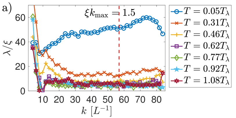
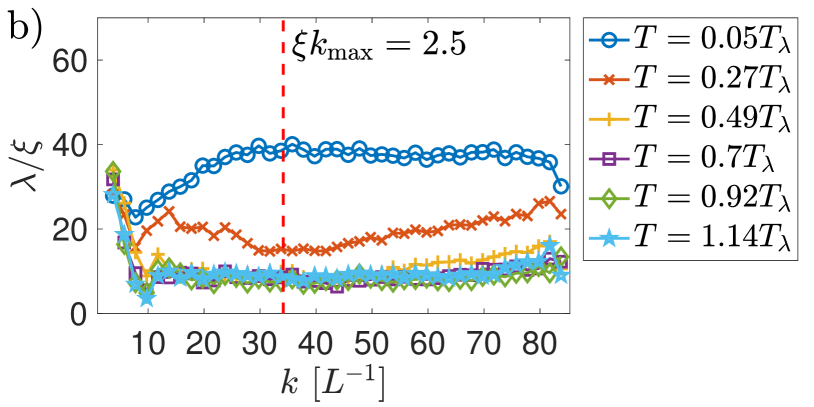
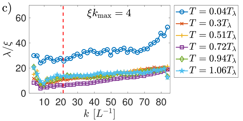
Figure 13: (Color online) Mean free-path as a function of $k$ for different temperatures in simulations with $\xi k_{\rm max}=1.5$ (a), $\xi k_{\rm max}=2.5$ (b) and $\xi k_{\rm max}=4$ (c). The vertical dashed line indicates the value of $1/\xi$.

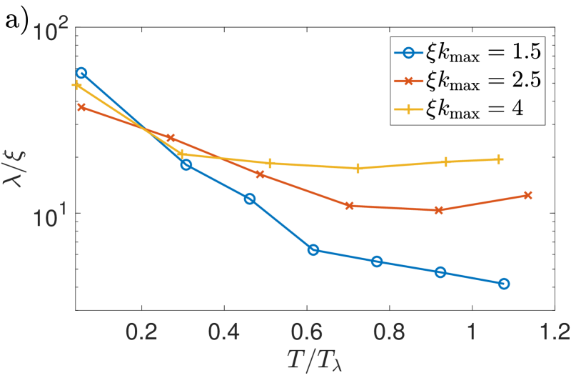
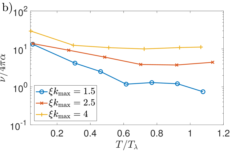
Figure 14: (Color online) (a) Mean free-path as a function of temperature $T$ for different values of $\xi k_{\rm max}$. (b) Effective viscosity (acting on the normal fluid), normalized by the quantum of circulation $4\pi\alpha=4\pi c\xi/\sqrt{2}$, as a function of temperature $T$ for different values of $\xi k_{\rm max}$.

In a two-fluid framework, the viscosity in Eq. (42) corresponds to a viscosity acting on the normal fluid (as it was obtained from the thermalized component). This is consistent with derivations of damping from stochastic equations for quasiclassical fields (see, e.g., Gardiner and Zoller (2000); Gardiner et al. (2002)), where modes below an energy cut-off are considered as the condensate, and modes above the cut-off are considered as thermalized noise. In our case the distinction is made using the STS, and from an extraction of the excitations lying in the vicinity of the dispersion relation of the waves. Thus, at very high temperatures we basically have one fluid with viscosity $\nu_{\rm eff}$. At intermediate temperatures, if the mutual friction is large enough, the two fluids are then locked together. Mutual friction in this case is estimated to be proportional to $\rho_{n}/\rho_{0}$ (see Krstulovic and Brachet (2011a)). Thus, at intermediate temperatures we can assume we have the fluids locked with an effective mutual viscosity

$$\nu_{\mathrm{eff}}^{\prime}=\frac{\rho_{n}(T)}{\rho_{0}}\nu_{\rm eff}(T).$$ (48)

These results are consistent with the following interpretation. On the one hand, at very large temperatures we have a very viscous flow. In the next subsection this will be verified by performing Navier-Stokes simulations using $\nu_{\mathrm{eff}}$ and comparing with runs of the TGPE. This will further confirm that the effective Reynolds numbers of flows in the TGPE are low even for the high resolution runs presented in this work, and also allow us to estimate the prefactor $C$ in Eq. (46). Moreover, this is also consistent with previous estimations based on the free decay of the incompressible kinetic energy in Clark Di Leoni et al. (2018). In fact, based on the estimation in Eq. (46), to obtain a turbulent normal fluid described by the TGPE near or above $T_{\lambda}$, would require resolutions that are not achievable even in the largest supercomputers available today (thus, doing a classical turbulent Navier-Stokes simulation with the TGPE can be very expensive!). On the other hand, at small temperatures we have a problem that could be modeled with the Euler and Boltzmann equations with small coupling, or more formally with a stochastic equation for a quasiclassical field Gardiner et al. (2002), with the system being close to GPE dynamics. Finally, in the middle region the system probably behaves close to Euler and Navier-Stokes fluids with coupling, and its modelling is left for future work.

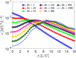
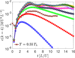
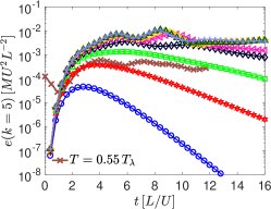
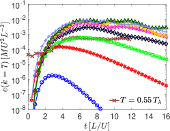
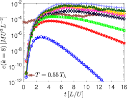
Figure 15: (Color online) Results from the DNS of low-Reynolds number Navier-Stokes TG runs at different Reynolds numbers (${\rm Re}=U_{0}L_{0}/\nu$, based on the integral scale $L_{0}$ and the flow r.m.s. velocity $U_{0}$, see Eqs.(44) and (45)). (a) Plots of energy dissipation rate $\epsilon$ vs time. The maximum of $\epsilon$ for the run with $Re=1860$ occurs at $t\approx 9\,L/U$. (b)-(f) Plots of the temporal evolution of the energy in different $k$-shells in Fourier space (i.e., $e(k,t)$ for fixed $k$ as a function of time) for $k=4$ to $8$ from the Navier-Stokes TG runs and the TGPE run at temperature $T=0.55\,T_{\lambda}$ (linear resolution $N=1024$ and $\xi k_{\rm max}=2.5$; for GPE $e(k,t)$ corresponds to $e^{i}_{\textrm{kin}}(k,t)$). In all panels, the GPE run at $T=0.55\,T_{\lambda}$ is indicated by the (brown) curve with crosses, while all Navier-Stokes runs at different Reynolds numbers are labeled as indicated in panel (a). To vary the Reynolds numbers, the Navier-Stokes runs were performed with kinematic viscosities $\nu=1/10$ and $\nu=1/40$ at linear spatial resolutions $N=64$; $\nu=1/80$ and $\nu=1/160$ ($N=128$); $\nu=1/320$, $\nu=1/640$ and $\nu=1/1280$ ($N=256$); $\nu=1/2560$ ($N=512$).

III.6 Comparisons with Low-Reynolds runs

To verify that the evolution of a finite temperature TG flow is similar to a highly viscous classical flow, and to estimate the value of the factor $C$ in Eq. (46), we perform a set of simulations of freely decaying “classical” TG flows obeying the Navier-Stokes equations at different Reynolds numbers, $\textrm{Re}=U_{0}L_{0}/\nu=7$ (with a spatial resolution $N^{3}=64^{3}$), 22 (with $64^{3}$ resolution), 53 ($128^{3}$), 110 ($128^{3}$), 240 ($256^{3}$), 480 ($256^{3}$), 950 ($256^{3}$), and 1860 ($512^{3}$). Here $\nu$ is the kinematic viscosity, and the r.m.s. flow velocity $U_{0}$ and the flow correlation length $L_{0}$ correspond to the averaged in time values between $t=4$ and $10$, when turbulence has developed. We compare these runs with the TGPE run at $T=0.55\,T_{\lambda}$ with linear resolution $N=1024$ and $\xi k_{\rm max}=2.5$.

In Fig. 15(a) we show the time evolution of the energy dissipation rate, $\epsilon$, for these TG Navier-Stokes runs. We observe that as we increase $\rm Re$, the time to achieve the maximum energy dissipation rate also increases, after which turbulence develops. To provide a detailed comparison between the runs, in Fig. 15 (b)-(f) we show the temporal evolution of the incompressible kinetic energy in Fourier shells $k=4\,L^{-1}$ to $8\,L^{-1}$, respectively, for the above mentioned Navier-Stokes runs and for the TGPE run. We find it remarkable that the shell by shell evolution of these two systems shows a considerable overlap for Reynolds numbers in the range $Re=22$ to $53$; in other words, the time evolution of the energy in each shell in the TGPE run is in between these two Navier-Stokes runs. This is in reasonable agreement, at least in terms of order of magnitude, with the predictions given by Eq. (46). Computing $L_{0}$ and $U_{0}$ in the TGPE run in the same time inverval (between $t=4$ and 10), we obtain $\textrm{Re}=5C$, suggesting $C\approx 7$.

IV Conclusion

The results presented in this paper significantly extend our knowledge of quantum turbulence in the Taylor-Green vortex. At zero temperature, runs in three dimensions computed with linear spatial resolutions up to $N=4096$ grid points allowed us to characterize the presence of a Kolmogorov scaling range at scales larger than the intervortex distance $\ell$, and to observe another scaling range at scales smaller than $\ell$. The presence of tangled substructures is apparent in vortex line visualizations.

Then, using thermal equilibria and spatio-temporal spectra, we were able to separate the condensed phase from the interacting waves, and to estimate from the nonlinear-broadening the mean free-path and the effective viscosity as a function of the temperature. The actual (large) values of our estimated effective viscosity near the $\lambda$-transition, $\nu_{\rm eff}\sim 500/N$ (in dimensionless units) for $\xi k_{\rm max}=2.5$, and $\nu_{\rm eff}\sim 90/N$ for $\xi k_{\rm max}=1.5$, correspond respectively to effective Reynolds numbers $\mathrm{Re}\sim U_{0}L_{0}N/500$ and $\mathrm{Re}\sim U_{0}L_{0}N/90$ (up to prefactors of order unity), where $N$ is the linear resolution of the simulation.

Finally, the comparison of finite temperature quantum turbulence using linear resolutions of $N=1024$ grid points against low-Reynolds Navier-Stokes numerical simulations further confirmed our estimations of the effective viscosity $\nu_{\rm eff}$ based on the mean free-path of the thermal excitations, and allowed us to get a first estimation of the amplitude of the unknown prefactors.

It is well known (see, e.g., Ref. Brachet et al. (1983)) that Kolmogorov scaling becomes apparent in Navier-Stokes numerical simulations of the Taylor-Green flow with linear resolutions of $N=256$, for $\mathrm{Re}\approx 1600$. We can thus conclude that an equivalent direct numerical simulation using the truncated Gross-Pitaevskii equation performed at $T\approx T_{\lambda}$ would need a resolution of about $N\approx 10,000$ grid points in each spatial direction for $\xi k_{\rm max}=1.5$, and of $N\approx 43,000$ for $\xi k_{\rm max}=2.5$, to achieve a similar Reynolds number and a classical direct energy cascade with similar scale separation for the normal fluid. These resolutions are out of reach using present day computing resources. At smaller values of $T$ this situation changes drastically, as the mutual friction between the fluid and the superfluid depends on the density of the normal fluid as $\rho_{n}/\rho_{0}$ Krstulovic and Brachet (2011a).

Looking back at the estimates of effective viscosity, it can be seen that the high value of $\nu_{\rm eff}$ traces back to the high value of $(d\omega_{B}/dk)^{2}/\Delta\omega$ at $k=k_{\rm max}$ for the Gross-Pitaevskii equation. This brings into mind the possibility of modifying the Bogoliubov dispersion relation through modifications in Gross-Pitaevskii, and therefore changing the value of $(d\omega_{B}/dk)^{2}$ at high wavenumbers. It is well known that, by changing the cubic term in the Gross-Pitaevskii equation into a non-local term of the form $\psi\int|\psi({\bf x^{\prime}})|^{2}V(|{\bf x-x^{\prime}}|)\,d{\bf x^{\prime}}$, the first term in the Bogoliubov dispersion relation can be changed to a term involving a potential $\widetilde{V}(k)=\int V(r)\exp[-i{\bf k}\cdot{\bf r}]\,d{\bf r}$. In this way, it is possible to “adjust” the dispersion relation, see, e.g., Eqs. (3) and (4) of Ref. Berloff et al. (2014). This, besides allowing the modeling of rotons in superfluid ⁴He at low temperatues, can also result in a decrease of the effective viscosity at temperatures close to the $\lambda$-transition. The impact of these changes in $\nu_{\rm eff}$ is left for future work.