Bifurcation in mean phase portraits for stochastic dynamical systems with multiplicative Gaussian noise

Abstract

We investigate the bifurcation phenomena for stochastic systems with multiplicative Gaussian noise, by examining qualitative changes in mean phase portraits. Starting from the Fokker-Planck equation for the probability density function of solution processes, we compute the mean orbits and mean equilibrium states. A change in the number or stability type, when a parameter varies, indicates a stochastic bifurcation. Specifically, we study stochastic bifurcation for three prototypical dynamical systems (i.e., saddle-node, transcritical, and pitchfork systems) under multiplicative Gaussian noise, and have found some interesting phenomena in contrast to the corresponding deterministic counterparts.

Key words:Stochastic bifurcation, Gaussian noise, Fokker-Planck equation, mean orbits, mean phase portraits

1 Introduction

Stochastic bifurcation is a phenomenon of qualitative changes in dynamical behaviors for stochastic systems, when a parameter varies [1, Ch.9]. One of the driving forces for studying stochastic bifurcation is that we want to know how a deterministic bifurcation differs under the influence of noise. Stochastic bifurcations have been observed in a wide range of complex systems in physical science and engineering [2, 3, 4, 5, 6].

Despite the fact that great progress has been made in the development of stochastic dynamical systems, the study of stochastic bifurcation is still in its infancy [7, 8]. A stochastic bifurcation may be defined as a qualitative change, such as the location, number and stability of equilibrium states in the evolution of a stochastic dynamical system, as a system parameter varies. Usually, a bifurcation diagram [9, 10, 11, 12] in terms of equilibrium states vs. bifurcation parameter is used to depict the qualitative changes in the phase space orbit structures for deterministic bifurcations in low dimensional dynamical systems. A bifurcation diagram thus represents the qualitative change of equilibrium states (or other geometrical invariant structures) vividly in phase portraits. However, the phase portrait for a stochastic dynamical system is a complicated matter, due to orbits’ dependency on random samples [13, Ch. 5]. More background in stochastic bifurcation is reviewed in our previous paper [14].

Arnold [1, Ch.9] considered stochastic bifurcations by examining changes in random attractors. Other existing works investigate stochastic bifurcation, for example, by examining the qualitative changes in random complete quasi-solutions [15], in invariant measures and their spectral stability [7, 8], in invariant measures with supports [16], in Conley index[17], or in logistic map[18]. Note that the invariant measures or Conley index are actually not in the state space (where orbits or phase portraits live). As in deterministic bifurcation, we would like to consider stochastic bifurcation in phase portraits. In our previous paper[14], we studied the stochastic bifurcation by examining the qualitative changes of equilibrium states in its most probable phase portraits[13, 19]. The most probable orbits indicate the most likely locations of dynamical orbits for a stochastic system.

In this present work, we examine stochastic bifurcation in mean phase portraits in state space. The mean orbits indicate the expected locations of the dynamical orbits. Sample solution orbits in phase portraits for stochastic differential equations are unintelligible objects. The phase portraits in terms of mean orbits [13, Ch.5] offer one promising option. Thus we propose to study stochastic bifurcation by examining the qualitative changes (especially the changes in the number, location and stability type for equilibrium states) in mean phase portraits. Specifically, we consider bifurcation for three prototypical scalar differential equations, i.e., saddle-node, transcritical, pitchfork systems, with multiplicative Brownian motion.

This letter is organized as follows. In Section 2, we define the mean phase portraits, and discuss the numerical methods for bifurcation diagrams. In Section 3, we present bifurcation diagrams for stochastic bifurcation under multiplicative Brownian motion in saddle-node, transcritical and pitchfork systems. We end this letter with a brief discussion in Section 4.

2 Methods

Consider a scalar stochastic differential equation with multiplicative Gaussian noise

$$dX_{t}=f(r,X_{t})dt+\sigma(X_{t})dB_{t},\;\;X_{0}=x_{0}.$$ (1)

where $f$ is a given vector field, $r$ is a real parameter, $\sigma$ is the noise intensity, and $B_{t}$ is a scalar Brownian motion.

The generator for this stochastic differential equation is

$$A\varphi(x)=f(r,x)\varphi^{\prime}(x)+\frac{1}{2}\sigma^{2}(x)\varphi^{\prime\prime}(x).$$ (2)

The Fokker-Planck equation for the probability density function $p(x,t)\triangleq p(x,t|x_{0},0)$ of the solution process $X_{t}$ with initial condition $X_{0}=x_{0}$ is [13]

$$p_{t}=A^{*}p,\;\;\;\;p(x,0)=\delta(x-x_{0}),$$ (3)

where $A^{*}$ is the adjoint operator of the generator $A$ in Hilbert space $L^{2}(\mathbb{R})$, and $\delta$ is the Dirac delta function. More specifically,

$$p_{t}=-(f(r,x)p(x,t))_{x}+\frac{1}{2}(\sigma^{2}(x)p(x,t))_{xx},\;\;\;p(x,0)=\delta(x-x_{0}).$$ (4)

We use a finite difference method [20] to simulate this Fokker-Planck equation (4) . The mean orbit starting at this initial point $x_{0}$ in the state space $\mathbb{R}$ is then computed by

$$\bar{X}(x_{0},t)=\int_{\mathbb{R}}\xi\;p(\xi,t|x_{0},0)d\xi.$$ (5)

A mean equilibrium state is a state which either attracts or repels all nearby mean orbits. When it attracts all nearby mean orbits, it is called a mean stable equilibrium state, while if it repels all nearby mean orbits, it is called a mean unstable equilibrium state. The mean phase portrait is composed of representative mean orbits, including mean equilibrium states.

Both mean phase portraits and mean equilibrium states are deterministic geometric objects. As in the study of bifurcation for deterministic dynamical systems [9, 10, 11], we examine the qualitative changes in the mean phase portraits, when a parameter varies. A simple stochastic bifurcation is the change in the ‘number’, ‘location’ or ‘stability type’ of mean equilibrium states in the mean phase portraits.

3 Results

In this section, we treat explicitly one-dimensional elementary and classical local bifurcations, namely stochastic saddle-node, transcritical and pitchfork bifurcation, in mean phase portraits. We generate bifurcation diagrams by examining the mean equilibrium states for these three prototypical stochastic systems under Gaussian noise, as a parameter $r$ in vector field varies.

As the rigorous general results for mean equilibrium states are lacking, we conduct numerical simulations to demonstrate the stochastic bifurcation phenomena.

3.1 Saddle-Node Bifurcation: $dX_{t}=(r+X_{t}^{2})dt+X_{t}dB_{t}$

First consider the stochastic saddle-node system $dX_{t}=f(r,X_{t})dt+\sigma(X_{t})dB_{t}$, with $f(r,X_{t})=r+X_{t}^{2}$ and $\sigma(X_{t})=X_{t}$.

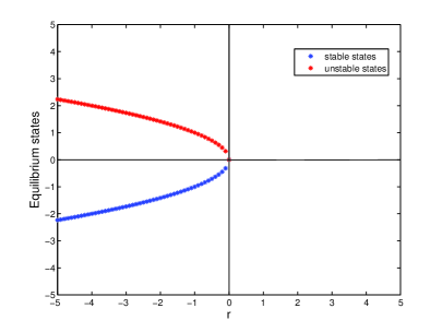
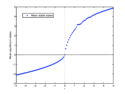
Figure 1: (Color online) Bifurcation diagrams for the saddle-node system: (a) Deterministic case (noise is absent); (b) Stochastic case.

Figure 1 is the well-known bifurcation diagram for the deterministic saddle-node system, i.e., equilibrium states vs. parameter $r$. Figure 1 is the bifurcation diagram for the stochastic system and it is the mean equilibrium states vs. parameter $r$.

We see that in the deterministic case, a bifurcation occurs at $r=0$. When $r$ is negative, there are two equilibrium states, one stable and one unstable; when $r=0$ the equilibrium states become a half stable equilibrium state; and when $r>0$, there are no equilibrium state at all. However, in the stochastic case, for $r>0$, there exists one positive mean stable state; for $r<0$, there exists one negative mean stable state; while for $r=0$, one mean equilibrium state is $x=0$. The location of mean equilibrium state varies as $r$ varies. A main difference occurs at $r>0$, where positive mean stable states emerge.

3.2 Transcritical Bifurcation: $dX_{t}=(rX_{t}-X_{t}^{2})dt+X_{t}dB_{t}$

Now consider the stochastic transcritical system $dX_{t}=f(r,X_{t})dt+\sigma(X_{t})dB_{t}$, with $f(r,X_{t})=rX_{t}-X_{t}^{2}$ and $\sigma(X_{t})=X_{t}$.

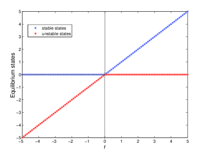
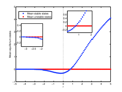
Figure 2: (Color online) Bifurcation diagrams for the transcritical system: (a) Deterministic case (noise is absent); (b) Stochastic case.

Figure 2 is the bifurcation diagram for the deterministic transcritical system. Figure 2 is the bifurcation diagram for the stochastic system :$dX_{t}=f(r,X_{t})dt+\sigma(X_{t})dB_{t}$, $f(r,X_{t})=rX_{t}-X_{t}^{2}$, $\sigma(X_{t})=X_{t}$.

In the deterministic case, it is the famous transcritical bifurcation. There is an equilibrium state at $x^{*}=0$ for all values of $r$. For $r<0$, there are two equilibrium states, one unstable at $x^{*}=r$ and the other stable at $x^{*}=0$; for $r=0$ , there is only one half stable equilibrium state $x^{*}=0$; while for $r>0$, there are also two equilibrium states, one unstable at $x^{*}=0$ and the other one stable at $x^{*}=r$. The two equilibrium states do not disappear after the bifurcation, they just switch their stability types.

In the stochastic case, the bifurcation is very different. When $r\lesssim-3$, there is only one mean stable point $x=0$, but for $r\gtrsim-3$, there are two mean equilibrium points: one mean stable point and one mean unstable point $0$. More specifically, the mean stable point is negative for$-3\lesssim r\gtrsim 0.8$, while the mean stable point is positive for $r\gtrsim 0.8$. The main difference occurs at $r\lesssim-3$, where there exists only one mean stable point $x=0$. From the details with enlarged scale in 2, we can see very clearly what happens around the bifurcation value.

3.3 Pitchfork Bifurcation: $dX_{t}=(rX_{t}-X_{t}^{3})dt+X_{t}dB_{t}$

Finally, we investigate the bifurcation for the stochastic pitchfork system $dX_{t}=f(r,X_{t})dt+\sigma(X_{t})dB_{t}$, with $f(r,X_{t})=rX_{t}-X_{t}^{3}$ and $\sigma(X_{t})=X_{t}$.

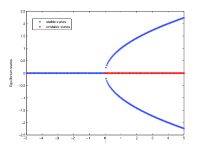
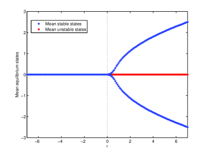
Figure 3: (Color online) Bifurcation diagrams for the pitchfork system: (a) Deterministic case (noise is absent); (b) Stochastic case.

Figure 3 is the bifurcation diagram for the deterministic pitchfork system. Figure 3 is the bifurcation diagram for the stochastic system:$dX_{t}=f(r,X_{t})dt+\sigma(X_{t})dB_{t}$, with $f(r,X_{t})=rX_{t}-X_{t}^{3}$ and $\sigma(X_{t})=X_{t}$.

Figure 3 shows the deterministic pitchfork system. For $r\leq 0$, $x=0$ is the only equilibrium state which is stable. While for $r>0$, there exist two stable equilibrium states $\sqrt{r}$ and $-\sqrt{r}$ and one unstable equilibrium state $x=0$. The bifurcation parameter value is $r=0$.

Figure 3 is for a type of stochastic pitchfork bifurcation, with the bifurcation value $r\approx 0.1$. It looks qualitatively similar to the deterministic one, but with a main difference in the bifurcation value, which is “delayed” due to the effects of noise.

4 Conclusion

For deterministic dynamical systems, we usually use their phase portraits to detect bifurcation. But for stochastic dynamical systems, the phase portraits are more delicate objects.

In this letter, we discuss stochastic bifurcation by examining the qualitative changes in mean equilibrium states in mean phase portraits. The mean orbits are computed by solving the corresponding Fokker-Planck equations for stochastic differential equations.

To demonstrate this stochastic bifurcation approach, we consider three prototypical systems under multiplicative Gaussian noise. We have observed that the deterministic bifurcations may be “altered” or “delayed” by noise. It is suggested that mean phase portraits, composed of representative mean orbits (especially mean equilibrium states), are intuitive and effective tools to detect stochastic bifurcation.

References

- [1] L. Arnold, Random Dynamical Systems New York Springer 1998 Corrected 2nd printing 2003
- [2] W. Horsthemke , R. Lefever , 2006 Noise-Induced Transitions. Berlin Heidelberg: Springer
- [3] G. Deco , D. Martí, 2007 Deterministic analysis of stochastic bifurcations in multi-stable neurodynamical systems. Biological Cybernetics, 96(5):487-496
- [4] W. Ebeling , I. M. Sokolov Statistical thermodynamics and stochastic theory of nonequilibrium systems . World Scientific, 2005.
- [5] J. Klafter, S.C. Lim, R. Metzler, 2011 Fractional Dynamics Singapore World Scientific.
- [6] R. Balescu, 1975 Equilibrium and nonequilibrium statistical mechanics Wiley.
- [7] H. Crauel, F. Flandoli, 1998 Additive noise destroys a pitchfork bifurcation J. Dyn. Diff. Eqn. 10 259-274
- [8] M. Callaway, T. S. Doan, J. S. W. Lamb, M. Rasmussen, 2017 The dichotomy spectrum for random dynamical systems and pitchfork bifurcations with additive noise Ann. Henri Poincaré.
- [9] J. Guckenheimer, P. Holmes, 1983 Nonlinear Oscillations, Dynamical Systems and Bifurcations of Vector Fields New York Springer
- [10] S. Wiggins, 2003 Introduction to Applied Nonlinear Dynamical Systems and Chaos Second Edition New York Springer
- [11] S. H. Strogatz, 1994 Nonlinear dynamics and chaos: with application to physics, biology, chemistry, and engineering New York Perseus Books
- [12] N. Sri. Namachchivaya, 1990 Stochastic bifurcation Applied Mathematics and Computation 39(3) 37-95
- [13] J. Duan 2015 An Introduction to Stochastic Dynamics New York Cambridge University Press
- [14] H. Wang, X. Chen and J.Duan 2018 A Stochastic Pitchfork Bifurcation in Most Probable Phase Portraits. International Journal of Bifurcation & Chaos, 28(1)
- [15] B. Wang, 2015 Stochastic bifurcation of pathwise random almost periodic and almost automorphic solutions for random dynamical systems Discrete and Continuous Dynamical Systems 35 (8) 3745 - 3769
- [16] K. Xu, 1995 Stochastic pitchfork bifurcation: numerical simulations and symbolic calculations using MAPLE Mathematics and Computers in Simulation 38 199-209
- [17] X. Chen, J. Duan, X. Fu, 2009 A sufficient condition for bifurcation in random dynamical systems Proceedings of the American Mathematical Society 138 965-973
- [18] Yet N. T., D. H. Son, T. Jäger and S. Siegmund , Nonautonomous saddle-Node bifurcations in the Quasiperiodically Forced logistic Map. International Journal of Bifurcation & Chaos, 2011, 21(05):1427-1438.
- [19] Z. Cheng , J. Duan , L. Wang, 2016 Most probable dynamics of some nonlinear systems under noisy fluctuatuons Commun. Nonlinear Sci. Numer. Simulat. 30:108-114
- [20] T. Gao, J. Duan, X. Li, 2016 Fokker-Planck equations for stochastic dynamical systems with symmetric Lévy motions Appl. Math. Comput. 278:1-20