Direct inversion of the nonequispaced fast Fourier transform

Abstract

Various applications such as MRI, solution of PDEs, etc. need to perform an inverse nonequispaced fast Fourier transform (NFFT), i. e., compute $M$ Fourier coefficients from given $N$ nonequispaced data. In the present paper we consider direct methods for the inversion of the NFFT. We introduce algorithms for the setting $M=N$ as well as for the underdetermined and overdetermined cases. For the setting $M=N$ a direct method of complexity $\mathcal{O}(N\log N)$ is presented, which utilizes Lagrange interpolation and the fast summation. For the remaining cases, we use the matrix representation of the NFFT to deduce our algorithms. Thereby, we are able to compute an inverse NFFT up to a certain accuracy by means of a modified adjoint NFFT in $\mathcal{O}(M\log M+N)$ arithmetic operations. Finally, we show that these approaches can also be explained by means of frame approximation.

1 Introduction

The NFFT, short hand for nonequispaced fast Fourier transform or nonuniform fast Fourier transform (NUFFT), respectively, is a fast algorithm to evaluate a trigonometric polynomial

$$f(x)=\sum_{k=-\frac{M}{2}}^{\frac{M}{2}-1}\hat{f}_{k}\,\mathrm{e}^{2\pi\mathrm{i}kx}$$ (1.1)

for given Fourier coefficients $\hat{f}_{k}\in\mathbb{C}$, $k=-\frac{M}{2},\dots,\frac{M}{2}-1$, $M\in 2\mathbb{N}$, at nonequispaced points $x_{j}\in\left[-\frac{1}{2},\frac{1}{2}\right)$, $\,j=1,\dots,N$. In case we are given equispaced points and $M=N$, this evaluation can be realized by means of the fast Fourier transform (FFT). For this setting also an algorithm for the inverse problem is known. Hence, we are interested in an inversion also for nonequispaced data, i. e., the Fourier coefficients $\hat{f}_{k}$ shall be computed for given function values $f_{j}=f(x_{j})$ of the trigonometric polynomial (1.1). Additionally, we study the inversion of the adjoint problem, namely the reconstruction of function values $f_{j}\in\mathbb{C}$ from given data

$$h_{k}=\sum_{j=1}^{N}f_{j}\,\mathrm{e}^{-2\pi\mathrm{i}kx_{j}},\quad k=-\tfrac{M}{2},\dots,\tfrac{M}{2}-1.$$ (1.2)

In general, the number $N$ of nodes $x_{j}$ is independent from the number $M$ of Fourier coefficients $\hat{f}_{k}$ and therefore the nonequispaced Fourier matrix

$$\boldsymbol{A}\coloneqq\left(\mathrm{e}^{2\pi\mathrm{i}kx_{j}}\right)_{j=1,\,k=-\frac{M}{2}}^{N,\;\frac{M}{2}-1}\ \in\mathbb{C}^{N\times M},$$ (1.3)

which we would have to invert, is rectangular in most cases. Nevertheless, several approaches have been developed to compute an inverse NFFT (iNFFT). First of all, there are some iterative methods. Recently, in [27] an algorithm was published for the setting $M=N$ which is based on the CG method as well as low rank approximation and is specially designed for jittered equispaced points. An approach for the overdetermined case can be found in [12], where the solution is computed iteratively by means of the CG algorithm using the Toeplitz structure of $\boldsymbol{A}^{*}\boldsymbol{W}\boldsymbol{A}$ with a diagonal matrix $\boldsymbol{W}$ of Voronoi weights. In [23] the CG method in connection with the NFFT was used to formulate an iterative algorithm for the underdetermined setting which deploys $\boldsymbol{A}\boldsymbol{\hat{W}}\boldsymbol{A}^{*}$ with weights $\boldsymbol{\hat{W}}$ based on kernel approximation. Furthermore, already in [11] a direct method was explained for the setting $M=N$ which uses Lagrange interpolation as well as fast multipole methods. Based on this, in [28] another direct method was deduced for the same setting which also uses Lagrange interpolation but additionally incorporates an imaginary shift for the fast evaluation of occurring sums. Since $\boldsymbol{A}^{*}\boldsymbol{A}$ is a Toeplitz matrix another direct method for the overdetermined setting can be derived using this special structure, see [18], analogously to [3]. In addition, also a frame-theoretical approach is known from [15] which provides a link between the adjoint NFFT and frame approximation and could therefore be seen as a method to invert the NFFT.

In this paper we present new direct methods for inverting the NFFT in general. For the quadratic setting, i. e., $M=N$, we review our method introduced in [21], which is also based on Lagrange interpolation but utilizes the fast summation to evaluate occurring sums. For the general case, we use as a motivation that for equispaced points an inversion can be realized by $\boldsymbol{A}\boldsymbol{A}^{*}\approx M\boldsymbol{I}_{N}$ and aim to generalize this result to find a good approximation of the inversion for nonequispaced nodes. To this end, we employ the decomposition $\boldsymbol{A}\approx\boldsymbol{B}\boldsymbol{F}\boldsymbol{D}$ known from the NFFT approach and compute the sparse matrix $\boldsymbol{B}$ such that we receive an approximation of the form $\boldsymbol{A}\boldsymbol{D}^{*}\boldsymbol{F}^{*}\boldsymbol{B}^{*}\approx M\boldsymbol{I}_{N}$. In other words, we are able to compute an inverse NFFT by means of a modified adjoint NFFT. Analogously, an inverse adjoint NFFT can be obtained by modifying the NFFT. Hence, the inversions can be computed in $\mathcal{O}(M\log M+N)$ arithmetic operations. The necessary precomputations developed in this paper are of complexity $\mathcal{O}(N^{2})$ and $\mathcal{O}(M^{2})$, respectively. Therefore, our method is especially beneficial in case we are given fixed nodes for several problems. Finally, we show that these approaches can also be explained by means of frame approximation.

The present work is organized as follows. In Section 2 we introduce the already mentioned algorithm, the NFFT. Afterwards, in Section 3 we deal with the inversion of this algorithm. In Section 3.1 we firstly review our method from [21] for the quadratic setting $M=N$. Secondly, in Section 3.2 the underdetermined and overdetermined settings are studied, which are treated separately in Sections 3.2.1 and 3.2.2. Finally, in Section 4 we deduce an approach for the inversion which is based on frame theory. Therefore, first of all, the main ideas of frames and approximation via frames will be introduced in Section 4.1 and subsequently, in Section 4.2, we will use these ideas to develop an approach for the iNFFT adapted from [15]. In the end, we will see that this frame-theoretical approach can be traced back to the methods for the inversion introduced in Section 3.2.

2 Nonequispaced fast Fourier transform

For given nodes $x_{j}\in\left[-\frac{1}{2},\frac{1}{2}\right)$,  $j=1,\dots,N$, $M\in 2\mathbb{N}$, as well as arbitrary Fourier coefficients $\hat{f_{k}}\in\mathbb{C},$ $k=-\frac{M}{2},\dots,\frac{M}{2}-1,$ we consider the computation of the sums

$$f_{j}=f(x_{j})=\sum_{k=-\frac{M}{2}}^{\frac{M}{2}-1}\hat{f_{k}}\,\mathrm{e}^{2\pi\mathrm{i}kx_{j}},\quad j=1,\dots,N,$$ (2.1)

as well as the adjoint problem of the computation of the sums (1.2) for given values $f_{j}\in\mathbb{C}$. A fast algorithm to solve this problem is called nonequispaced fast Fourier transform (NFFT) and is briefly explained below, cf. [10, 5, 29, 26, 25, 16, 20, 27].

By defining the matrix (1.3) as well as the vectors $\boldsymbol{f}\coloneqq\left(f_{j}\right)_{j=1}^{N}$, $\boldsymbol{\hat{f}}\coloneqq(\hat{f}_{k})_{k=-\frac{M}{2}}^{\frac{M}{2}-1}$ and $\boldsymbol{h}\coloneqq(h_{k})_{k=-\frac{M}{2}}^{\frac{M}{2}-1}$, the computation of sums of the form (2.1) and (1.2) can be written as $\boldsymbol{f}=\boldsymbol{A}\boldsymbol{\hat{f}}$ and $\boldsymbol{h}=\boldsymbol{A}^{*}\boldsymbol{f}$, where $\boldsymbol{A}^{*}=\overline{\boldsymbol{A}}^{\mathrm{T}}$ denotes the adjoint matrix of $\boldsymbol{A}$.

2.1 The NFFT

We firstly restrict our attention to problem (2.1), which is equivalent to the evaluation of a trigonometric polynomial $f$ at nodes $x_{j}$, see (1.1). At first, we approximate $f$ by a linear combination of translates of a 1-periodic function $\tilde{w}$, i. e.,

$$f(x)\approx s_{1}(x)\coloneqq\sum_{l=-\frac{M_{\sigma}}{2}}^{\frac{M_{\sigma}}{2}-1}g_{l}\,\tilde{w}\left(x-\tfrac{l}{M_{\sigma}}\right),$$

where $M_{\sigma}=\sigma M$ with the so-called oversampling factor $\sigma\geq 1$. In the easiest case $\tilde{w}$ originates from periodization of a function $w\colon[-\frac{1}{2},\frac{1}{2})\to\mathbb{R}$. Let this so-called window function be chosen such that its 1-periodic version $\tilde{w}(x)=\sum_{r\in\mathbb{Z}}w(x+r)$ has an absolutely convergent Fourier series. By means of the definition

$$\hat{g}_{k}\coloneqq\sum_{l=-\frac{M_{\sigma}}{2}}^{\frac{M_{\sigma}}{2}-1}g_{l}\,\mathrm{e}^{-2\pi\mathrm{i}kl/{M_{\sigma}}},\quad k\in\mathbb{Z},$$

and the convolution theorem, $s_{1}$ can be represented as

$$s_{1}(x) =\sum_{k=-\infty}^{\infty}c_{k}(s_{1})\,\mathrm{e}^{2\pi\mathrm{i}kx}$$ (2.2)

$$=\sum_{k=-\frac{M_{\sigma}}{2}}^{\frac{M_{\sigma}}{2}-1}\hat{g}_{k}\;c_{k}(\tilde{w})\,\mathrm{e}^{2\pi\mathrm{i}kx}+\sum_{r=-\infty\atop{r\neq 0}}^{\infty}\sum_{k=-\frac{M_{\sigma}}{2}}^{\frac{M_{\sigma}}{2}-1}\hat{g}_{k}\;c_{k+M_{\sigma}r}(\tilde{w})\,\mathrm{e}^{2\pi\mathrm{i}(k+M_{\sigma}r)x}.$$

Comparing (2.1) and (2.2) gives rise for the following definition. We set

$$\hat{g}_{k}\coloneqq\left\{\begin{array}[]{cl}\dfrac{\hat{f}_{k}}{\hat{w}(k)}&:k\in\{-\frac{M}{2},\dots,\frac{M}{2}-1\},\\ 0&:k\in\{-\frac{M_{\sigma}}{2},\dots,\frac{M_{\sigma}}{2}-1\}\setminus\{-\frac{M}{2},\dots,\frac{M}{2}-1\},\end{array}\right.$$

where the Fourier transform of $w$ is given by

$$\hat{w}(k)=\int_{-\infty}^{\infty}w(x)\,\mathrm{e}^{-2\pi\mathrm{i}kx}\,\mathrm{d}x=\int_{-\frac{1}{2}}^{\frac{1}{2}}\tilde{w}(x)\,\mathrm{e}^{-2\pi\mathrm{i}kx}\,\mathrm{d}x=c_{k}(\tilde{w}).$$ (2.3)

Furthermore, we suppose $w$ is small outside the interval $\left[-\nicefrac{{m}}{{M_{\sigma}}},\nicefrac{{m}}{{M_{\sigma}}}\right]$,  $m\ll M_{\sigma}.$ Then $w$ can be approximated by $w_{m}(x)=\chi_{\left[-\nicefrac{{m}}{{M_{\sigma}}},\nicefrac{{m}}{{M_{\sigma}}}\right]}\cdot w(x)$, which is compactly supported since $\chi_{\left[-\nicefrac{{m}}{{M_{\sigma}}},\nicefrac{{m}}{{M_{\sigma}}}\right]}$ denotes the characteristic function of $\left[-\nicefrac{{m}}{{M_{\sigma}}},\nicefrac{{m}}{{M_{\sigma}}}\right].$ Thus, $\tilde{w}$ can be approximated by the 1-periodic function $\tilde{w}_{m}$ with

$$\sum_{k\in\mathbb{Z}}\hat{w}(k)\,\mathrm{e}^{2\pi\mathrm{i}kx}=\tilde{w}(x)\approx\tilde{w}_{m}(x)=\sum_{r\in\mathbb{Z}}w_{m}(x+r).$$

Hence, we obtain the following approximation

$$f(x_{j})\approx s_{1}(x_{j})\approx s(x_{j})\coloneqq\sum_{l=-\frac{M_{\sigma}}{2}}^{\frac{M_{\sigma}}{2}-1}g_{l}\,\tilde{w}_{m}\left(x_{j}-\tfrac{l}{M_{\sigma}}\right)=\sum_{l=\lceil M_{\sigma}x_{j}\rceil-m}^{\lfloor M_{\sigma}x_{j}\rfloor+m}g_{l}\,\tilde{w}_{m}\left(x_{j}-\tfrac{l}{M_{\sigma}}\right),$$

where simplification arises because many summands vanish. By defining

• the diagonal matrix

  $$\boldsymbol{D}\coloneqq\text{diag}\left(\frac{1}{M_{\sigma}\hat{w}(k)}\right)_{k=-\frac{M}{2}}^{\frac{M}{2}-1}\ \in\mathbb{C}^{M\times M},$$ (2.4)

• the truncated Fourier matrix

  $$\boldsymbol{F}\coloneqq\left(\mathrm{e}^{2\pi\mathrm{i}k\frac{l}{M_{\sigma}}}\right)_{l=-\frac{M_{\sigma}}{2},\,k=-\frac{M}{2}}^{\frac{M_{\sigma}}{2}-1,\;\frac{M}{2}-1}\ \in\mathbb{C}^{M_{\sigma}\times M},$$ (2.5)

• and the sparse matrix

  $$\boldsymbol{B}\coloneqq\bigg{(}\tilde{w}_{m}\left(x_{j}-\tfrac{l}{M_{\sigma}}\right)\bigg{)}_{j=1,\,l=-\frac{M_{\sigma}}{2}}^{N,\;\frac{M_{\sigma}}{2}-1}\ \in\mathbb{R}^{N\times M_{\sigma}},$$ (2.6)

this can be formulated in matrix-vector notation and we receive the approximation $\boldsymbol{A}\approx\boldsymbol{B}\boldsymbol{F}\boldsymbol{D}$. Therefore, the corresponding fast algorithm consisting of three steps is of complexity $\mathcal{O}(M\log M+N)$.

Remark 2.1.

Suitable window functions can be found in [10, 5, 29, 9, 13, 16, 20].       

Remark 2.2.

It must be pointed out that because of consistency the factor $\frac{1}{M_{\sigma}}$ is here not located in the matrix $\boldsymbol{F}$ as usual but in the matrix $\boldsymbol{D}$.       

2.2 The adjoint NFFT

Now we consider the problem (1.2), which is treated similarly to [26], and therefore we firstly define the function

$$\tilde{g}(x)\coloneqq\sum_{j=1}^{N}f_{j}\,\tilde{w}(x_{j}-x)$$ (2.7)

and calculate its Fourier coefficients

$$c_{k}(\tilde{g}) =\int_{-\frac{1}{2}}^{\frac{1}{2}}\tilde{g}(x)\,\mathrm{e}^{-2\pi\mathrm{i}kx}\,\mathrm{d}x=\sum_{j=1}^{N}f_{j}\,\mathrm{e}^{-2\pi\mathrm{i}kx_{j}}\int_{-\frac{1}{2}}^{\frac{1}{2}}\tilde{w}(y)\,\mathrm{e}^{2\pi\mathrm{i}ky}\,\mathrm{d}y=h_{k}\,c_{-k}(\tilde{w}).$$

In other words, the values $h_{k}$ can be computed if $c_{-k}(\tilde{w})$ and $c_{k}(\tilde{g})$ are known. The Fourier coefficients of $\tilde{g}$ are determined approximately by means of the trapezoidal rule

$$c_{k}(\tilde{g})\approx\frac{1}{M_{\sigma}}\sum_{l=-\frac{M_{\sigma}}{2}}^{\frac{M_{\sigma}}{2}-1}\sum_{j=1}^{N}f_{j}\,\tilde{w}\left(x_{j}-\tfrac{l}{M_{\sigma}}\right)\,\mathrm{e}^{-2\pi\mathrm{i}kl/M_{\sigma}}.$$

Let the function $w$ moreover be well localized in time so that $\tilde{w}$ can be replaced by $\tilde{w}_{m}$ again. Then we obtain the approximation

$$\frac{c_{k}(\tilde{g})}{c_{-k}(\tilde{w})}\approx\frac{1}{M_{\sigma}\hat{w}(-k)}\sum_{l=-\frac{M_{\sigma}}{2}}^{\frac{M_{\sigma}}{2}-1}\sum_{j=1}^{N}f_{j}\,\tilde{w}_{m}\left(x_{j}-\tfrac{l}{M_{\sigma}}\right)\,\mathrm{e}^{-2\pi\mathrm{i}kl/M_{\sigma}}\eqqcolon\tilde{h}_{k}.$$ (2.8)

Rewriting this by means of (2.4), (2.5) and (2.6) we receive $\boldsymbol{A}^{*}\approx\boldsymbol{D}^{*}\boldsymbol{F}^{*}\boldsymbol{B}^{*}$. Hence, the algorithm for the adjoint problem is also of complexity $\mathcal{O}(M\log M+N)$.

3 Inversion of the NFFT

Having introduced the fast methods for nonequispaced data, we aim to find an inversion for these algorithms encouraged by the fact that for equispaced data the inversion is well-known. Therefore, we face the following two problems.

1. Solve

   $$\begin{split}\boldsymbol{A}\boldsymbol{\hat{f}}&=\boldsymbol{f},\\ \text{ given: }\boldsymbol{f}\in\mathbb{C}^{N},&\text{ find: }\boldsymbol{\hat{f}}\in\mathbb{C}^{M},\end{split}$$ (3.1)

   i. e., reconstruct the Fourier coefficients $\boldsymbol{\hat{f}}=(\hat{f}_{k})_{k=-\frac{M}{2}}^{\frac{M}{2}-1}$ from given function values $\boldsymbol{f}=(f_{j})_{j=1}^{N}$. This will be solved by an inverse NFFT.

2. Solve

   $$\begin{split}\boldsymbol{A}^{*}\boldsymbol{f}&=\boldsymbol{h},\\ \text{ given: }\boldsymbol{h}\in\mathbb{C}^{M},&\text{ find: }\boldsymbol{f}\in\mathbb{C}^{N},\end{split}$$ (3.2)

   i. e., reconstruct the coefficients $\boldsymbol{f}=(f_{j})_{j=1}^{N}$ from given data $\boldsymbol{h}=(h_{k})_{k=-\frac{M}{2}}^{\frac{M}{2}-1}$. This will be solved by an inverse adjoint NFFT.

In both problems the numbers $M$ and $N$ are independent. It is obvious that except for the quadratic setting $M=N$ there are two different ways to choose $M$ and $N$. The first possibility is $M<N$, i. e., for the inverse NFFT in (3.1) we are given more function values than Fourier coefficients, which we are supposed to find. That means, we are in an overdetermined setting. The second variation is the converse setting $M>N$, where we have to find more Fourier coefficients than we are given initial data. Hence, this is the underdetermined case. Analogously, the same relations can be considered for the inverse adjoint NFFT in (3.2). There $M$ belongs to the given data whereas $N$ goes with the wanted solution. Thus, the overdetermined case in now $M>N$ while the problem is underdetermined for $M<N$.

This section is organized as follows. Firstly, in Section 3.1 the inversions are derived for the quadratic case $M=N$. Secondly, in Section 3.2.1 we survey the underdetermined case of the inverse NFFT, which corresponds to the overdetermined case of the adjoint. Finally, in Section 3.2.2 the overdetermined case of the inverse NFFT is explained, which is related to the underdetermined case of the adjoint.

3.1 The quadratic case

For the quadratic case $M=N$ we use an approach analogous to [11, 28], where an inversion is realized by means of Lagrange interpolation. While the fast algorithms are obtained in [11] by means of FMM, our method from [21] employs the fast summation for acceleration, see [25].

The main idea is to use a relation between two evaluations of a trigonometric polynomial

$$f_{j}\coloneqq f(y_{j})=\sum_{k=-\frac{N}{2}}^{\frac{N}{2}-1}\hat{f}_{k}\,\mathrm{e}^{2\pi\mathrm{i}ky_{j}},\quad j=1,\dots,N,$$

and

$$g_{l}\coloneqq f(x_{l})=\sum_{k=-\frac{N}{2}}^{\frac{N}{2}-1}\hat{f}_{k}\,\mathrm{e}^{2\pi\mathrm{i}kx_{l}},\quad l=1,\dots,N,$$ (3.3)

for different nodes $x_{l},y_{j}\in\left[-\frac{1}{2},\frac{1}{2}\right)$, $l,j=1,\dots,N,$ and Fourier coefficients $\hat{f}_{k}\in\mathbb{C}$,  $k=-\frac{N}{2},\dots,\frac{N}{2}-1$. By defining the coefficients

$$a_{l}=\prod_{n=1}^{N}\sin(\pi(x_{l}-y_{n}))\quad\text{ and }\quad b_{j}=\prod_{n=1\atop{n\neq j}}^{N}\frac{1}{\sin(\pi(y_{j}-y_{n}))},\quad l,j=1,\dots,N,$$ (3.4)

we observe the relation

$$g_{l}=a_{l}\sum_{j=1}^{N}f_{j}\,b_{j}\left(\frac{1}{\tan(\pi(x_{l}-y_{j}))}-\mathrm{i}\right),\quad l=1,\dots,N,$$ (3.5)

cf. [11, Theorem 2.3]. Hence, for given nonequispaced nodes $y_{j}$ the computation of an inverse NFFT can be realized by choosing additional points $x_{l}$ and applying formula (3.5). If these nodes $x_{l}$ are chosen equidistantly we can compute the Fourier coefficients $\hat{f}_{k}$ by simply applying an FFT to the coefficients $g_{l}$ in (3.3).

Remark 3.1.

It must be pointed out that the considered approach is only applicable for disjoint sets of nodes. If this condition is violated this would mean division by zero in case of the coefficients $b_{j}$, cf. (3.4). However, this can easily be avoided since we are free to choose the equispaced points $x_{l}$ distinct from $y_{j}$.       

We approximate the coefficients $g_{l}$ in (3.5) by using the fast summation, see [25]. Considering the computation scheme we see that it is possible to compute

$$\tilde{g}_{l}\coloneqq\sum_{j=1}^{N}f_{j}\,b_{j}\cot(\pi(x_{l}-y_{j})),\quad l=1,\dots,N,$$ (3.6)

by means of the fast summation. Then the wanted coefficients $g_{l}$ can be obtained by

$$g_{l}=a_{l}\left(\tilde{g}_{l}-\mathrm{i}\cdot\sum_{j=1}^{N}f_{j}\,b_{j}\right),\quad l=1,\dots,N,$$ (3.7)

where we only have to compute an additional scalar product of two vectors, which requires only $\mathcal{O}(N)$ arithmetic operations. Considering the kernel $K(x)=\cot(\pi x)$ in detail it becomes apparent that this function has not only a singularity at $x=0$ but also at the boundary $x=\pm 1$. Thus, we have to make an effort. For detailed information about the computation see [21].

The coefficients $a_{l}$ and $b_{j}$ can also be computed efficiently by the fast summation because of the observations

$$\tilde{a}_{l}\coloneqq\ln|a_{l}|=\ln\left|\,\prod_{n=1}^{N}\sin(\pi(x_{l}-y_{n}))\right|=\sum_{n=1}^{N}\,\ln\left|\sin(\pi(x_{l}-y_{n}))\right|$$

and

$$\tilde{b}_{j}\coloneqq\ln|b_{j}| =\ln\left|\,\prod_{n=1\atop{n\neq j}}^{N}\frac{1}{\sin(\pi(y_{j}-y_{n}))}\right|=-\sum_{n=1\atop{n\neq j}}^{N}\,\ln\left|\sin(\pi(y_{j}-y_{n}))\right|.$$

Therefore, it is possible to use the kernel $K(x)=\ln(|\sin(\pi x)|)$ to compute the absolute values and perform a sign correction afterwards to receive the signed coefficients $a_{l}$ and $b_{j}$. Having a closer look at the kernel it becomes apparent that this function is also one-periodic and shows singularities at the same positions as the cotangent does. Hence, the computation works analogously.

Remark 3.2.

A straightforward implementation of (3.5) can lead to overflow and underflow issues. The closer our nodes are the more formula (3.5) suffers from these issues. However, having a look at the coefficients $a_{l}$ and $b_{j}$ we recognize that the decrease and the increase are in the same scale. Thus, for $s\in\mathbb{R}$ we realize a stabilization by considering $|a_{l}|\cdot|b_{j}|=\mathrm{e}^{\ln|a_{l}|}\,\mathrm{e}^{\ln|b_{j}|}=\mathrm{e}^{\tilde{a}_{l}}\,\mathrm{e}^{\tilde{b}_{j}}=\mathrm{e}^{\tilde{a}_{l}+s}\,\mathrm{e}^{\tilde{b}_{j}-s},$ i. e., instead of computing products of the coefficients we use the additional factor $\mathrm{e}^{s}$ to overcome numerical difficulties. To bring the coefficients as close together as possible we choose $s=\min\left\{\min_{j}\{\tilde{d}_{j}\},\min_{l}\{\tilde{c}_{l}\}\right\}$. For details see also [19, ./matlab/infft1d].       

Thus, we obtain the following fast algorithm.

Algorithm 3.3 (Fast inverse NFFT - quadratic case).

  
For $N\in 2\mathbb{N}$ let be given equispaced nodes $x_{l}\in\left[-\frac{1}{2},\frac{1}{2}\right),\,l=1,\dots,N$, nonequispaced nodes $y_{j}\in\left[-\frac{1}{2},\frac{1}{2}\right)$ and $f_{j}\in\mathbb{C},\,j=1,\dots,N$.

1. Compute $\tilde{a}_{l}=\ln|a_{l}|$ and $\tilde{b}_{j}=\ln|b_{j}|$ by means of the fast summation using the kernel function $K(x)=\ln(|\sin(\pi x)|)$. $\mathcal{O}(N\log N)$

2. Determine the stabilization factor $s$ and set $a_{l}=\mathrm{e}^{\tilde{a}_{l}+s}$ and $b_{j}=\mathrm{e}^{\tilde{b}_{j}-s}$. $\mathcal{O}(N)$

3. Perform a sign correction for $a_{l}$ and $b_{j}$. $\mathcal{O}(N)$
   (If the nodes have to be sorted, we end up with $\mathcal{O}(N\log N)$)

4. Compute $\tilde{g}_{l}$ analogously to $\tilde{a}_{l}$ by means of the fast summation with the kernel function $K(x)=\cot(\pi x)$, cf. (3.6). $\mathcal{O}(N\log N)$

5. Compute $g_{l}$ via (3.7). $\mathcal{O}(N)$

6. Compute

   $$\check{f}_{k}=\frac{1}{N}\sum_{l=1}^{N}g_{l}\,\mathrm{e}^{-2\pi\mathrm{i}kx_{l}},\quad k=-\tfrac{N}{2},\dots,\tfrac{N}{2}-1,$$

   by means of an FFT. $\mathcal{O}(N\log N)$

Output: $\check{f}_{k}\approx\hat{f}_{k}$
Complexity: $\mathcal{O}(N\log N)$  
 

Remark 3.4.

This algorithm is part of the software package NFFT 3.4.1, see [19, ./matlab/infft1d].       

Now we have a look at some numerical examples.

Example 3.5.

We choose arbitrary Fourier coefficients $\hat{f}_{k}\in[1,100]$ and compute the evaluations of the related trigonometric polynomial (1.1). Out of these we want to retrieve the given $\hat{f}_{k}$. As mentioned in [15, 8, 1] we examine so-called jittered equispaced nodes

$$y_{j}=-\frac{1}{2}+\frac{j-1}{N}+\frac{1}{4N}\,\theta,\quad j=1,\dots,N,\ \text{with}\ \theta\sim U(0,1),$$ (3.8)

where $U(0,1)$ denotes the uniform distribution on the interval $(0,1)$ and the factor $\frac{1}{4}$ is our choice for the arbitrary perturbation parameter which has to be less than $\frac{1}{2}$ in order to not let the nodes switch position. For a detailed study of this sampling pattern we refer to [1, Section 4]. We consider the absolute and relative errors per node

$$\frac{e_{r}^{\mathrm{abs}}}{N}=\frac{1}{N}\|\boldsymbol{\hat{f}}-\boldsymbol{\check{f}}\|_{r}\quad\text{ and }\quad\frac{e_{r}^{\mathrm{rel}}}{N}=\frac{\|\boldsymbol{\hat{f}}-\boldsymbol{\check{f}}\|_{r}}{N\,\|\boldsymbol{\hat{f}}\|_{r}}$$ (3.9)

for $r\in\{2,\infty\}$, where $\boldsymbol{\check{f}}$ is the outcome of Algorithm 3.3.

As a first experiment we use $N=2^{c}$ with $c=1,\dots,14$, and for the parameters needed in the fast summation we use the standard values, see [19]. In a second experiment we fix $N=1024$ and increase some of the standard values, namely the cut-off parameter $m$ and the degree of smoothness $p$ shall be chosen uniformly $m=p=c$ with $c=4,\dots,12$.

The corresponding results are depicted in Figure 3.1. Having a look at the errors per node for growing $N$, see (a), we observe that the errors are worse if we consider very small sizes of $N$. Otherwise, we recognize that these errors remain stable for large sizes of $N$. In (b) we can see that for fixed $N$ a higher accuracy can be achieved by tuning the parameters of the fast summation.

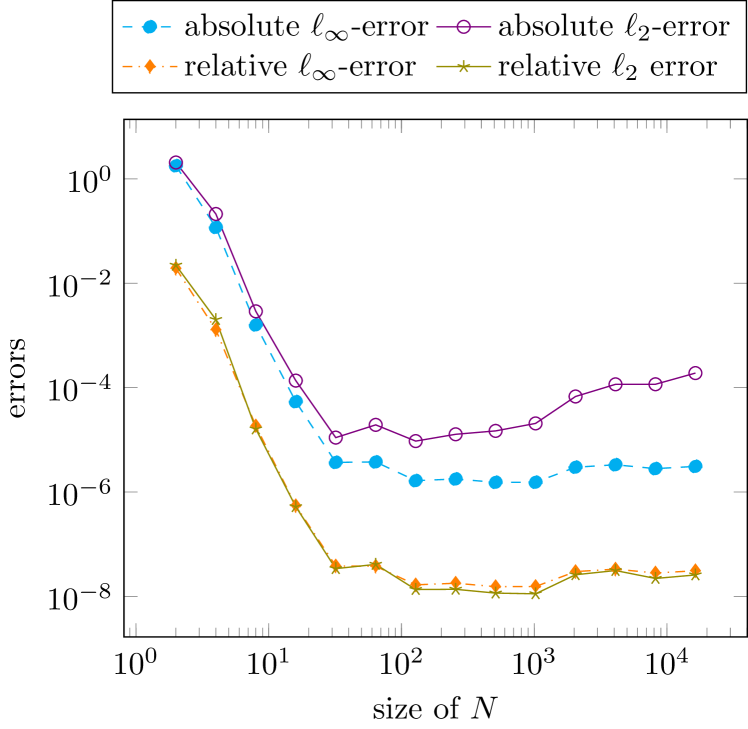
(a) $N=2^{c},\,c=1,\dots,14,$
and $m=p=4$.

(b) $N=1024$ and
$m=p=c,\,c=4,\dots,12$.

Figure 3.1: Comparison of the errors per node (3.9) of reconstructed Fourier coefficients generated by Algorithm 3.3 for jittered equispaced nodes.

      

Remark 3.6.

We have a look at the condition number of the nonequispaced Fourier matrix $\boldsymbol{A}$. Figure 3.2 displays $\mathrm{cond}_{2}(\boldsymbol{A})=\|\boldsymbol{A}\|_{2}\|\boldsymbol{A}^{-1}\|_{2}$ for different kinds of nodes for increasing $N=2^{c},\,c=1,\dots,10$. There we see that the distribution of the nonequispaced nodes is of great importance. For jittered equispaced nodes, cf. (3.8), the condition number is nearly 1 for all sizes of $N$, so this problem is well-conditioned. However, for Chebyshev nodes

$$y_{j}=\frac{1}{2}\cos\left(\frac{2(N-j)+1}{2N}\ \pi\right),\quad j=1,\dots,N,$$ (3.10)

or logarithmically spaced nodes

$$y_{j}=\left(\frac{6}{5}\right)^{j-N},\quad j=1,\dots,N,$$

it is easy to see that the condition number rises rapidly. These last mentioned problems are simply ill-conditioned and we cannot assume a good approximation by Algorithm 3.3. For a detailed investigation of the condition number for rectangular nonequispaced Fourier matrices see [22] and the references therein and also [4, 6].

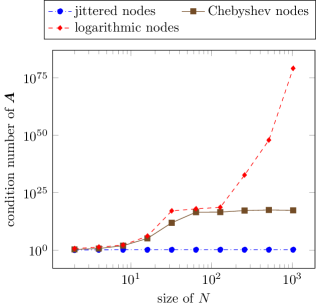
Figure 3.2: Comparison of condition numbers of the nonequispaced Fourier matrix $\boldsymbol{A}$ computed using cond from MATLAB for different kinds of nodes for $N=2^{c},\,c=1,\dots,10$.

      

Remark 3.7.

We obtain an inverse adjoint NFFT by simply considering the adjoint of Algorithm 3.3, i. e., for $\boldsymbol{v}\coloneqq(v_{l})_{l=1}^{N}$ being the inverse Fourier transform of $\boldsymbol{h}$ we apply the formula

$$f_{j}=b_{j}\sum_{l=1}^{N}a_{l}\,v_{l}\left(\frac{1}{\tan(\pi(x_{l}-y_{j}))}+\mathrm{i}\right),\quad j=1,\dots,N.$$ (3.11)

This relation can easily be seen by using the matrix representation of Algorithm 3.3.       

3.2 The rectangular case

For the general case $M\neq N$ we follow a different approach. To clarify the idea we firstly have a look at equispaced nodes

$$x_{j}=\tfrac{j}{N}\in\left[-\tfrac{1}{2},\tfrac{1}{2}\right),\,j=-\tfrac{N}{2},\dots,\tfrac{N}{2}-1.$$

Thereby, we obtain

$$\boldsymbol{A}=\left(\mathrm{e}^{2\pi\mathrm{i}k\frac{j}{N}}\right)_{j=-\frac{N}{2},\,k=-\frac{M}{2}}^{\frac{N}{2}-1,\;\frac{M}{2}-1}\quad\text{ and }\quad\boldsymbol{A}^{*}=\left(\mathrm{e}^{-2\pi\mathrm{i}k\frac{j}{N}}\right)_{k=-\frac{M}{2},\,j=-\frac{N}{2}}^{\frac{M}{2}-1,\;\frac{N}{2}-1}.$$

Considering products of these two matrices it becomes apparent that $\boldsymbol{A}^{*}\boldsymbol{A}=N\boldsymbol{I}_{M}$ for $M\leq N$ as well as $\boldsymbol{A}\boldsymbol{A}^{*}=M\boldsymbol{I}_{N}$ for $M\geq N$ with $N\mid M$. This is to say, in these special cases we are given an inversion of the NFFT by composition of the Fourier matrices. Hence, we seek to use this result to find a good approximation of the inversion in the general case. This will be done by modification of the matrix $\boldsymbol{B}$ so that we receive an approximation of the form $\boldsymbol{A}\boldsymbol{D}^{*}\boldsymbol{F}^{*}\boldsymbol{B}^{*}\approx M\boldsymbol{I}_{N}$ similar to the equispaced case. For this purpose, the entries of the matrix $\boldsymbol{B}$ should be calculated such that its sparse structure with at most $(2m+1)$ entries per row and consequently the arithmetic complexity of the algorithms is preserved. A matrix $\boldsymbol{B}$ satisfying this property we call (2m+1)-sparse.

It is to be noticed that the fact of underdetermination and overdetermination is not of great importance when deducing the methods for the inversion. Even if it is a necessary condition for the exact inversion for equispaced nodes, the algorithms in the nonequispaced setting can always be used in both cases. However, we will see later on that each algorithm works best in one of these cases and therefore they are already introduced for this special case. Having this in mind we give an outline of how to handle problems (3.1) and (3.2).

1. To solve (3.1) our aim is to compute a sparse matrix $\boldsymbol{B}^{*}$ from given nodes $x_{j}$ such that by application of an adjoint NFFT we obtain a fast inverse NFFT.

   Suppose we are given the approximation $\boldsymbol{A}\boldsymbol{D}^{*}\boldsymbol{F}^{*}\boldsymbol{B}^{*}\approx M\boldsymbol{I}_{N}$. Then it also holds that

   $$\frac{1}{M}\ \boldsymbol{A}\boldsymbol{D}^{*}\boldsymbol{F}^{*}\boldsymbol{B}^{*}\boldsymbol{f}\approx\boldsymbol{f}\quad\forall\boldsymbol{f}\in\mathbb{C}^{N}.$$ (3.12)

   If we now set

   $$\boldsymbol{\check{f}}:=\frac{1}{M}\,\boldsymbol{D}^{*}\boldsymbol{F}^{*}\boldsymbol{B}^{*}\boldsymbol{f},$$

   we can rewrite approximation (3.12) as $\boldsymbol{A}\boldsymbol{\check{f}}\approx\boldsymbol{f}$. Since we already know that $\boldsymbol{A}\boldsymbol{\hat{f}}=\boldsymbol{f}$ this means $\boldsymbol{\check{f}}\approx\boldsymbol{\hat{f}}$, which could be interpreted as a reconstruction of the Fourier coefficients $\boldsymbol{\hat{f}}$. To achieve a good approximation we want $\boldsymbol{\check{f}}$ to be as close as possible by $\boldsymbol{\hat{f}}$. This can be accomplished by optimizing $\boldsymbol{A}\boldsymbol{\check{f}}\approx\boldsymbol{f}$, i. e., we aim to solve the optimization problem

   $$\underset{\boldsymbol{\check{f}}\in\mathbb{C}^{M}}{\text{Minimize }}\ \|\boldsymbol{A}\boldsymbol{\check{f}}-\boldsymbol{f}\|_{2}.$$

   Using the definition of $\boldsymbol{\check{f}}$ this norm can be estimated above by

   $$\|M\boldsymbol{A}\boldsymbol{\check{f}}-M\boldsymbol{f}\|_{2}=\|\boldsymbol{A}\boldsymbol{D}^{*}\boldsymbol{F}^{*}\boldsymbol{B}^{*}\boldsymbol{f}-M\boldsymbol{f}\|_{2}\leq\|\boldsymbol{A}\boldsymbol{D}^{*}\boldsymbol{F}^{*}\boldsymbol{B}^{*}-M\boldsymbol{I}_{N}\|_{\mathrm{F}}\,\|\boldsymbol{f}\|_{2},$$

   where the Frobenius norm is denoted by $\|\cdot\|_{\mathrm{F}}$. Because $\boldsymbol{f}$ is given, this expression can be minimized by solving

   $$\underset{\boldsymbol{B}\in\mathbb{R}^{N\times M_{\sigma}}\colon\boldsymbol{B}\,(2m+1)\text{-sparse }}{\text{Minimize }}\ \|\boldsymbol{A}\boldsymbol{D}^{*}\boldsymbol{F}^{*}\boldsymbol{B}^{*}-M\boldsymbol{I}_{N}\|_{\mathrm{F}}^{2}.$$ (3.13)

2. To solve (3.2) we aim to compute a sparse matrix $\boldsymbol{B}$ from given nodes $x_{j}$ such that by application of an NFFT we obtain a fast inverse adjoint NFFT.

   Again we suppose $\boldsymbol{A}\boldsymbol{D}^{*}\boldsymbol{F}^{*}\boldsymbol{B}^{*}\approx M\boldsymbol{I}_{N}$, which is equivalent to its adjoint

   $$\boldsymbol{B}\boldsymbol{F}\boldsymbol{D}\boldsymbol{A}^{*}\approx M\,\boldsymbol{I}_{N}\quad\text{and\ }\quad\frac{1}{M}\,\boldsymbol{B}\boldsymbol{F}\boldsymbol{D}\,(\boldsymbol{A}^{*}\boldsymbol{f})\approx\boldsymbol{f}\quad\forall\boldsymbol{f}\in\mathbb{C}^{N},$$

   respectively. Because we know $\boldsymbol{h}=\boldsymbol{A}^{*}\boldsymbol{f}$, this could be interpreted as a reconstruction of the coefficients $\boldsymbol{f}$. To achieve a good approximation we solve the optimization problem

   $$\underset{\boldsymbol{B}\in\mathbb{R}^{N\times M_{\sigma}}\colon\boldsymbol{B}\,(2m+1)\text{-sparse }}{\text{Minimize }}\ \|\boldsymbol{B}\boldsymbol{F}\boldsymbol{D}\boldsymbol{h}-M\boldsymbol{f}\|_{2},$$

   where the norm could be estimated as follows.

   $$\|\boldsymbol{B}\boldsymbol{F}\boldsymbol{D}\boldsymbol{h}-M\boldsymbol{f}\|_{2}=\|\boldsymbol{B}\boldsymbol{F}\boldsymbol{D}\boldsymbol{A}^{*}\boldsymbol{f}-M\boldsymbol{f}\|_{2}\leq\|\boldsymbol{B}\boldsymbol{F}\boldsymbol{D}\boldsymbol{A}^{*}-M\boldsymbol{I}_{N}\|_{\mathrm{F}}\,\|\boldsymbol{f}\|_{2}.$$

   Hence, we end up with the optimization problem

   $$\underset{\boldsymbol{B}\in\mathbb{R}^{N\times M_{\sigma}}\colon\boldsymbol{B}\,(2m+1)\text{-sparse }}{\text{Minimize }}\ \|\boldsymbol{B}\boldsymbol{F}\boldsymbol{D}\boldsymbol{A}^{*}-M\boldsymbol{I}_{N}\|_{\mathrm{F}}^{2}.$$

So, all in all, with the chosen approach we are able to generate an inverse NFFT as well as an inverse adjoint NFFT by modifying the matrices $\boldsymbol{B}^{*}$ and $\boldsymbol{B}$, respectively, and applying an adjoint NFFT or an NFFT with these modified matrices.

Remark 3.8.

We investigate below if the reconstruction error can be reduced by appropriate choice of the entries of the matrix $\boldsymbol{B}$. Already in [24] the minimization of the Frobenius norm $\|\boldsymbol{A}-\boldsymbol{BFD}\|_{\textrm{F}}$ was analyzed regarding a sparse matrix $\boldsymbol{B}$ to achieve a minimum error for the NFFT. In contrast, we study the minimization of $\|\boldsymbol{A}\boldsymbol{D}^{*}\boldsymbol{F}^{*}\boldsymbol{B}^{*}-M\boldsymbol{I}_{N}\|_{\textrm{F}}^{2}$ to achieve a minimum error for the inverse NFFT as well as the minimization of $\|\boldsymbol{B}\boldsymbol{F}\boldsymbol{D}\boldsymbol{A}^{*}-M\boldsymbol{I}_{N}\|_{\textrm{F}}^{2}$ to achieve a minimum error for the inverse adjoint NFFT.       

3.2.1 Inverse NFFT – underdetermined case

We start deducing our inversion as outlined in general. However, in the numerical experiments in Examples 3.13 and 3.14 we will see that this method is especially beneficial for the underdetermined setting and hence it is already attributed to this case.

As mentioned before we aim to find a solution for (3.1) by solving (3.13). Therefore, we consider the matrix $\boldsymbol{A}\boldsymbol{D}^{*}\boldsymbol{F}^{*}\boldsymbol{B}^{*}$ for given nodes $x_{j}\in\mathbb{T}$,  $j=1,\dots,N$. Apparently, we have

$$\boldsymbol{A}\boldsymbol{D}^{*}\boldsymbol{F}^{*}=\left[\frac{1}{M_{\sigma}}\sum_{k=-\frac{M}{2}}^{\frac{M}{2}-1}\frac{1}{\hat{w}(-k)}\,\mathrm{e}^{2\pi\mathrm{i}k\left(x_{j}-\frac{l}{M_{\sigma}}\right)}\right]_{j=1,\,l=-\frac{M_{\sigma}}{2}}^{N,\frac{M_{\sigma}}{2}-1}.$$ (3.14)

By defining the “inverse window function”

$$K(x)=\frac{1}{M_{\sigma}}\sum_{k=-\frac{M}{2}}^{\frac{M}{2}-1}\frac{1}{\hat{w}(-k)}\,\mathrm{e}^{2\pi\mathrm{i}kx}$$ (3.15)

we receive

$$\boldsymbol{K}\coloneqq\boldsymbol{A}\boldsymbol{D}^{*}\boldsymbol{F}^{*}=\left(K\left(x_{h}-\tfrac{l}{M_{\sigma}}\right)\right)_{h=1,\,l=-\frac{M_{\sigma}}{2}}^{N,\ \frac{M_{\sigma}}{2}-1}.$$

Having a look at the matrix $\boldsymbol{B}^{*}$ it becomes apparent that there are only a few nonzero entries. Thus, we study the window $\tilde{w}_{m}$ for further simplification. For $w_{m}$ we have $\text{supp}(w_{m})=\left[-\tfrac{m}{M_{\sigma}},\tfrac{m}{M_{\sigma}}\right]$, i. e., for the 1-periodic version $\tilde{w}_{m}(x):=\sum_{z\in\mathbb{Z}}w_{m}(x+z)$ it holds

$$\tilde{w}_{m}\left(x_{j}-\tfrac{l}{M_{\sigma}}\right)\neq 0 \iff\exists\,z\in\mathbb{Z}:\ -m\leq M_{\sigma}x_{j}-l+M_{\sigma}z\leq m.$$

By defining the set

$$I_{M_{\sigma},m}(x_{j})\coloneqq\left\{l\in\left\{-\tfrac{M_{\sigma}}{2},\dots,\tfrac{M_{\sigma}}{2}-1\right\}:\exists\,z\in\mathbb{Z}\ \text{with}-m\leq M_{\sigma}x_{j}-l+M_{\sigma}z\leq m\right\}$$ (3.16)

we can therefore write

$$\left(\boldsymbol{A}\boldsymbol{D}^{*}\boldsymbol{F}^{*}\boldsymbol{B}^{*}\right)_{h,j} =\sum_{k=-\frac{M}{2}}^{\frac{M}{2}-1}\mathrm{e}^{2\pi\mathrm{i}kx_{h}}\left(\sum_{l\in I_{M_{\sigma},m}(x_{j})}\frac{1}{M_{\sigma}\hat{w}(-k)}\,\mathrm{e}^{-2\pi\mathrm{i}k\frac{l}{M_{\sigma}}}\ \tilde{w}_{m}\left(x_{j}-\tfrac{l}{M_{\sigma}}\right)\right).$$

Hence, our considered norm can be written as

$$\|\boldsymbol{A}\boldsymbol{D}^{*} \boldsymbol{F}^{*}\boldsymbol{B}^{*}-M\boldsymbol{I}_{N}\|_{\textrm{F}}^{2}=$$ (3.17)

$$=\sum_{h=1}^{N}\sum_{j=1}^{N}\left|\ \sum_{k=-\frac{M}{2}}^{\frac{M}{2}-1}\mathrm{e}^{2\pi\mathrm{i}kx_{h}}\left(\sum_{l\in I_{M_{\sigma},m}(x_{j})}\frac{1}{M_{\sigma}\hat{w}(-k)}\,\mathrm{e}^{-2\pi\mathrm{i}k\frac{l}{M_{\sigma}}}\,\tilde{w}_{m}\left(x_{j}-\tfrac{l}{M_{\sigma}}\right)\right)-M\delta_{hj}\right|^{2}.$$

Based on the definition of the Frobenius norm of a matrix $\boldsymbol{A}\in\mathbb{R}^{k\times n}$ we obtain for $\boldsymbol{a}_{j}$ being columns of $\boldsymbol{A}\in\mathbb{R}^{k\times n}$ that

$$\|\boldsymbol{A}\|_{F}^{2}=\sum_{i=1}^{k}\sum_{j=1}^{n}|a_{ij}|^{2}=\sum_{j=1}^{n}\|\boldsymbol{a}_{j}\|_{2}^{2}.$$

This yields that (3.17) can be rewritten by means of

$$\boldsymbol{T}_{j}=\left(\mathrm{e}^{-2\pi\mathrm{i}k\frac{l}{M_{\sigma}}}\right)_{k=-\frac{M}{2},\,l\in I_{M_{\sigma},m}(x_{j})}^{\frac{M}{2}-1},\quad\boldsymbol{b}_{j}=\bigg{(}\tilde{w}_{m}\left(x_{j}-\tfrac{l}{M_{\sigma}}\right)\bigg{)}_{l\in I_{M_{\sigma},m}(x_{j})}$$

and $\boldsymbol{e}_{j}=(\delta_{hj})_{h=1}^{N}$ as

$$\|\boldsymbol{A}\boldsymbol{D}^{*}\boldsymbol{F}^{*}\boldsymbol{B}^{*}-M\boldsymbol{I}_{N}\|_{\textrm{F}}^{2}=\sum_{j=1}^{N}\|\boldsymbol{A}\boldsymbol{D}^{*}\boldsymbol{T}_{j}\boldsymbol{b}_{j}-M\boldsymbol{e}_{j}\|_{2}^{2}.$$ (3.18)

Therefore, the considered norm in (3.13) is minimal if and only if $\|\boldsymbol{A}\boldsymbol{D}^{*}\boldsymbol{T}_{j}\boldsymbol{b}_{j}-M\boldsymbol{e}_{j}\|_{2}^{2}$ is minimal for all $j=1,\dots,N$. Hence, we obtain the optimization problems

$$\underset{\tilde{\boldsymbol{b}}_{j}\in\mathbb{R}^{2m+1}}{\text{Minimize }}\ \|\boldsymbol{A}\boldsymbol{D}^{*}\boldsymbol{T}_{j}\tilde{\boldsymbol{b}}_{j}-M\boldsymbol{e}_{j}\|_{2}^{2},\quad j=1,\dots,N,$$ (3.19)

since the columns of the matrix $\boldsymbol{B}^{*}$ contain at most $(2m+1)$ nonzeros. Thus, if

$$\boldsymbol{K}_{j}\coloneqq\boldsymbol{A}\boldsymbol{D}^{*}\boldsymbol{T}_{j}=\left[\frac{1}{M_{\sigma}}\sum_{k=-\frac{M}{2}}^{\frac{M}{2}-1}\frac{1}{\hat{w}(-k)}\,\mathrm{e}^{2\pi\mathrm{i}k\left(x_{h}-\frac{l}{M_{\sigma}}\right)}\right]_{h=1,\,l\in I_{M_{\sigma},m}(x_{j})}^{N}\in\mathbb{C}^{N\times(2m+1)}$$ (3.20)

has full rank the solution of problem (3.19) is given by

$$\tilde{\boldsymbol{b}}_{j}=M\left(\boldsymbol{K}_{j}^{*}\boldsymbol{K}_{j}\right)^{-1}\boldsymbol{K}_{j}^{*}\boldsymbol{e}_{j},\quad j=1,\dots,N.$$ (3.21)

For generating the modified matrix $\boldsymbol{B}_{\mathrm{opt}}^{*}$ it must be pointed out that the vectors $\tilde{\boldsymbol{b}}_{j}$ only contain the $(2m+1)$ nonzeros of the columns of $\boldsymbol{B}_{\mathrm{opt}}^{*}$. Hence, attention must be paid to the periodicity which can also be seen in the structure of the matrix $\boldsymbol{B}^{*}$.

Remark 3.9.

Whether the matrix $\boldsymbol{K}_{j}$ has full rank only depends on the matrix $\boldsymbol{A}$. The conditions when this matrix has full rank can e. g. be found in [17] and [23].       

Next we develop a method for the fast computation of $\tilde{\boldsymbol{b}}_{j}$. It is already known from Section 2 that sums of the form (2.1) can be computed in $\mathcal{O}(M\log M+N)$ arithmetic operations for given nodes $x_{j}\in\left[-\frac{1}{2},\frac{1}{2}\right)$, $j=1,\dots,N,$ and coefficients $\hat{f}_{k}\in\mathbb{C},\,k=-\frac{M}{2},\dots,\frac{M}{2}-1$. If we have a look at the matrix $\boldsymbol{K}_{j}$, cf. (3.20), it becomes apparent that we can compute its entries by means of the NFFT with coefficients

$$\hat{f}_{k}=\frac{1}{M_{\sigma}\hat{w}(-k)},\quad k=-\tfrac{M}{2},\dots,\tfrac{M}{2}-1,$$ (3.22)

and nodes $y_{h,l}\coloneqq x_{h}-\tfrac{l}{M_{\sigma}},\,h=1,\dots,N,l\in I_{M_{\sigma},m}(x_{j})$, which are at most $N(2m+1)$ many. If we put the columns of $\boldsymbol{K}_{j}$ one below the other into a vector, we are able to compute these entries only using one NFFT of length $N(2m+1)$. In so doing, we have to reshape the obtained vector into a matrix afterwards.

Another point to mention is that the coefficients $\hat{f}_{k}$ are the same for the computation of all matrices $\boldsymbol{K}_{j}$,$\,j=1,\dots,N$. This is to say, we can precompute step 1 and step 2 of the NFFT since there only information about the Fourier coefficients $\hat{f}_{k}$ is needed, cf. [26]. Merely for the last step of the NFFT we need the current nodes and therefore this step has to be performed separately for every $j=1,\dots,N$. Thus, we receive the following algorithm.

Algorithm 3.10 (Fast optimization of the matrix $\boldsymbol{B}^{*}$).

  
For $N\in\mathbb{N}$ let $x_{j}\in\left[-\frac{1}{2},\frac{1}{2}\right),\,j=1,\dots,N,$ be given nodes as well as $M\in 2\mathbb{N}$, $\sigma\geq 1$ and $M_{\sigma}=\sigma M$. Furthermore, we are given the oversampling factor $\sigma_{2}\geq 1$ and the cut-off parameter $m_{2}$ for an NFFT.

1. Compute $\boldsymbol{g}=\boldsymbol{F}\boldsymbol{D}\boldsymbol{\hat{f}}$, cf. (2.4) and (2.5), with $\hat{f}_{k}$ in (3.22). $\mathcal{O}(M\log M)$

2. For $j=1,\dots,N$:

   • Determine the set $I_{M_{\sigma},m}(x_{j})$, cf. (3.16). $\mathcal{O}(1)$

   • Perform $\boldsymbol{B}\boldsymbol{g}$, cf. (2.6), for the vector of nodes

     $$\boldsymbol{y}\coloneqq\left(\boldsymbol{y}_{1}^{T},\dots,\boldsymbol{y}_{s}^{T}\right)^{T}$$

     for $\boldsymbol{y}_{n}$ being the columns of the matrix $\boldsymbol{Y}\coloneqq(y_{h,l})_{h=1,\,l\in I_{M_{\sigma},m}(x_{j})}^{N}$. $\mathcal{O}(N)$

   • Reshape the obtained vector into the matrix $\boldsymbol{K}_{j}\in\mathbb{C}^{N\times(2m+1)}$. $\mathcal{O}(N)$

   • Solve the normal equations for $\boldsymbol{K}_{j}$, cf. (3.21). $\mathcal{O}(N)$

3. Compose $\boldsymbol{B}_{\mathrm{opt}}^{*}$ column-wise of the vectors $\tilde{\boldsymbol{b}}_{j}$ observing the periodicity. $\mathcal{O}(N)$

Output: optimized matrix $\boldsymbol{B}_{\mathrm{opt}}^{*}$
Complexity: $\mathcal{O}(N^{2}+M\log{M})$  
 

Remark 3.11.

It is possible to simplify Algorithm 3.10 by replacing the inverse window function in (3.15) by the Dirichlet kernel

$$D_{\frac{M}{2}-1}(x)=\sum_{k=-\frac{M}{2}+1}^{\frac{M}{2}-1}\mathrm{e}^{2\pi\mathrm{i}kx}=\frac{\sin((M-1)\pi x)}{\sin(\pi x)}.$$ (3.23)

Hence, the entries of $\boldsymbol{K}_{j}$ in (3.20) can explicitly be stated by means of (3.23) as

$$\boldsymbol{K}_{j}=\left[\frac{1}{M_{\sigma}}\,D_{\frac{M}{2}-1}\left(x_{h}-\tfrac{l}{M_{\sigma}}\right)\right]_{h=1,\,l\in I_{M_{\sigma},m}(x_{j})}^{N}$$

and thereby the term $M\log M$ in the computational costs of Algorithm 3.10 is eliminated. Thus, we end up with an arithmetic complexity of $\mathcal{O}(N^{2})$.       

Remark 3.12.

This algorithm using a window function or the Dirichlet kernel is part of the software package NFFT 3.5.1, see [19, ./matlab/infft1d].       

Now we have a look at some numerical examples.

Example 3.13.

Firstly, we verify that the optimization was successful. To this end, we compare the norms

$$\|\boldsymbol{A}\boldsymbol{D}^{*}\boldsymbol{F}^{*}\boldsymbol{B}^{*}-M\boldsymbol{I}_{N}\|_{\textrm{F}}\quad\text{ and }\quad\|\boldsymbol{A}\boldsymbol{D}^{*}\boldsymbol{F}^{*}\boldsymbol{B}_{\mathrm{opt}}^{*}-M\boldsymbol{I}_{N}\|_{\textrm{F}},$$ (3.24)

where $\boldsymbol{B}^{*}$ denotes the original matrix from the adjoint NFFT and $\boldsymbol{B}_{\mathrm{opt}}^{*}$ the optimized matrix generated by Algorithm 3.10. Even though our method is attributed to the underdetermined setting, this is not a restriction. Hence, we also test for the overdetermined setting.

• Firstly, we choose $N=128$ jittered equispaced nodes, cf. (3.8), $M=2^{c}$ with $c=4,\dots,12,$ and for the NFFT in Algorithm 3.10 we choose the Kaiser-Bessel window, $\sigma_{2}=2.0$ and $m_{2}=2m$ to receive high accuracy. Figure 3.3 depicts the comparison of the norms (3.24) for different values of $m$ and $\sigma$ for $\boldsymbol{B}_{\mathrm{opt}}^{*}$ generated using B-Splines as well as the Dirichlet kernel as mentioned in Remark 3.11. It can be seen that the optimization was really successful for large values of $M$ compared to $N$ whereas the minimization does not work in the overdetermined setting $M<N$. But in fact, this is not surprising because then we try to approximate the identity by a low rank matrix since $\boldsymbol{A}\boldsymbol{D}^{*}\boldsymbol{F}^{*}\boldsymbol{B}^{*}\in\mathbb{C}^{N\times N}$ has at most rank $M$. Therefore, Algorithm 3.10 is specially attributed to the underdetermined case. We recognize that the optimization is worsened against expectation by using a higher oversampling factor $\sigma$ whereas increasing the cut-off $m$ expectedly leads to better results.

  Figure 3.4 displays the run-times of Algorithm 3.10 comparing B-Spline and Dirichlet kernel for $m=2$ and $\sigma=1.0$. It is obvious that the usage of the Dirichlet kernel considerably reduces the run-time. Since the results are the same for other parameters and window functions additional tests are omitted.

• Next we repeat the example for Chebyshev nodes, cf. (3.10). The corresponding outcomes for B-Splines can be found in Figure 3.5. There we see that the gap between $M$ and $N$ has to be huge to achieve results similar to those for jittered equispaced nodes.       

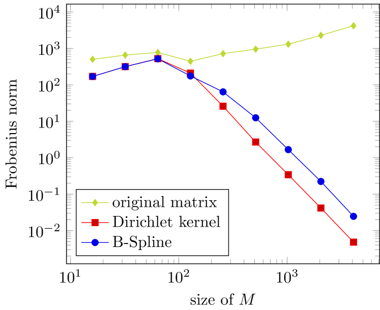
(a) $m=2$ and $\sigma=1.0$

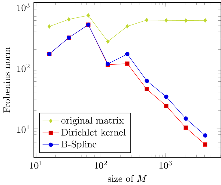
(b) $m=2$ and $\sigma=2.0$

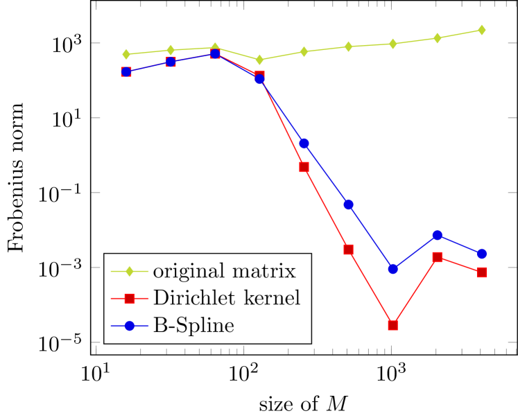
(c) $m=4$ and $\sigma=1.0$

Figure 3.3: Comparison of Frobenius norms (3.24) of the original matrix $\boldsymbol{B}^{*}$ and the optimized matrix $\boldsymbol{B}_{\mathrm{opt}}^{*}$ generated by Algorithm 3.10 using B-Spline window functions as well as the Dirichlet kernel for $N=128$ jittered equispaced nodes and $M=2^{c}$ with $c=4,\dots,12$.

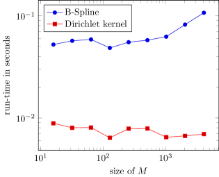
Figure 3.4: Comparison of run-times of Algorithm 3.10 using the B-Spline as well as the Dirichlet kernel with $m=2$ and $\sigma=1.0$ for $N=128$ jittered equispaced nodes and $M=2^{c}$ with $c=4,\dots,12$.

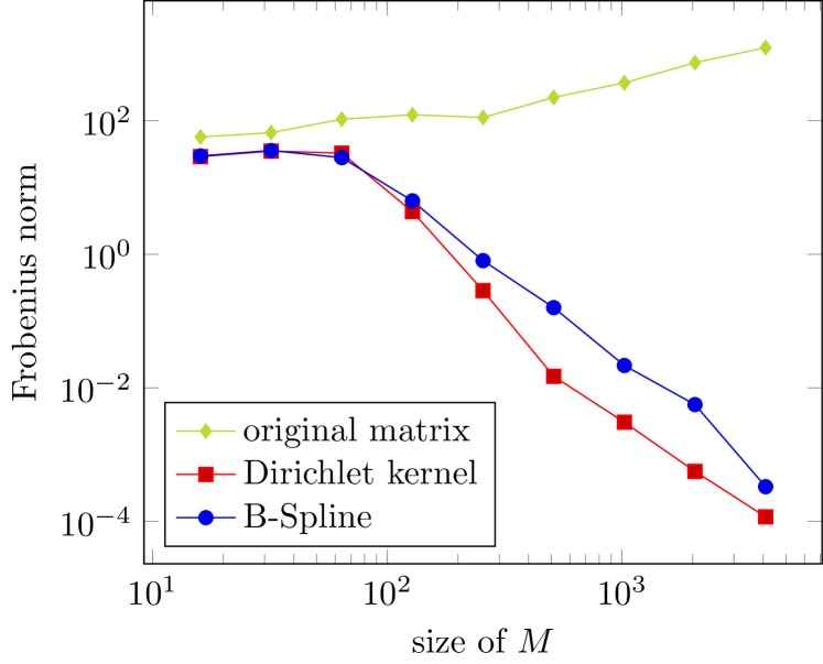
(a) $N=16$

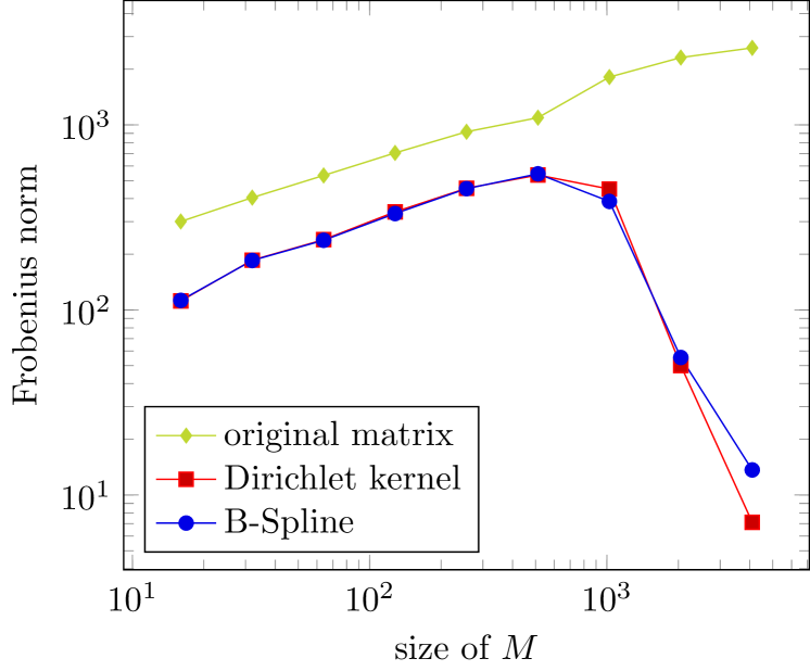
(b) $N=64$

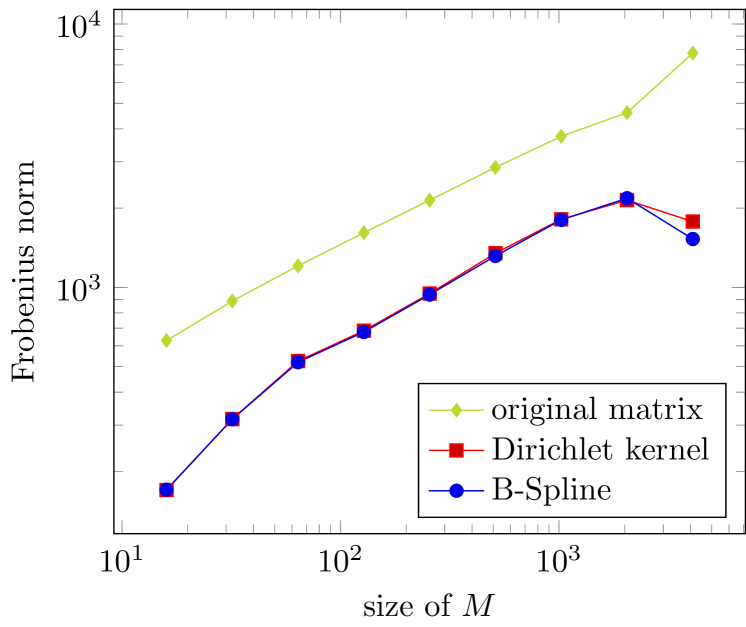
(c) $N=128$

Figure 3.5: Comparison of Frobenius norms (3.24) of the original matrix $\boldsymbol{B}^{*}$ and the optimized matrix $\boldsymbol{B}_{\mathrm{opt}}^{*}$ generated by Algorithm 3.10 using B-Spline window functions as well as the Dirichlet kernel with $m=2$ and $\sigma=1.0$ for different numbers of Chebyshev nodes and $M=2^{c}$ with $c=4,\dots,12$.

Example 3.14.

Secondly, we check if we can retrieve given Fourier coefficients from evaluations of the related trigonometric polynomial (1.1), cf. Example 3.5. For $\boldsymbol{f}=\left(f(x_{j})\right)_{j=1}^{N}$ with given nodes $x_{j}$ we consider the estimate $\boldsymbol{\check{f}}=\left(\check{f}_{k}\right)_{k=-\frac{M}{2}}^{\frac{M}{2}-1}=\frac{1}{M}\,\boldsymbol{D}^{*}\boldsymbol{F}^{*}\boldsymbol{B}_{\mathrm{opt}}^{*}\boldsymbol{f}$, where $\boldsymbol{B}_{\mathrm{opt}}^{*}$ is the output of Algorithm 3.10. Here we choose the Dirichlet kernel with $\sigma=2.0$ and jittered equispaced nodes $x_{j}$. We consider the absolute and relative errors per node

$$\frac{e_{r}^{\mathrm{abs}}}{N}=\frac{1}{N}\|\boldsymbol{A}\boldsymbol{\check{f}}-\boldsymbol{f}\|_{r}\quad\text{ and }\quad\frac{e_{r}^{\mathrm{rel}}}{N}=\frac{\|\boldsymbol{A}\boldsymbol{\check{f}}-\boldsymbol{f}\|_{r}}{N\,\|\boldsymbol{f}\|_{r}}$$ (3.25)

for $r\in\{2,\infty\}$. As a first experiment we use $N=2^{c}$ with $c=1,\dots,12$, $M=4N$, and $m=4$. In a second experiment we fix $N=512$ and $M=2048$ and the cut-off parameter $m$ shall be chosen $m=c$ with $c=4,\dots,12$. The corresponding results are depicted in Figure 3.6. Having a look at the errors per node for growing $N$, see (a), we observe that the errors are worse if we consider very small sizes of $N$. Otherwise, we recognize that these errors get smaller for large sizes of $N$. In (b) we can see that for fixed $N$ these errors remain quite stable when tuning the cut-off parameter $m$.

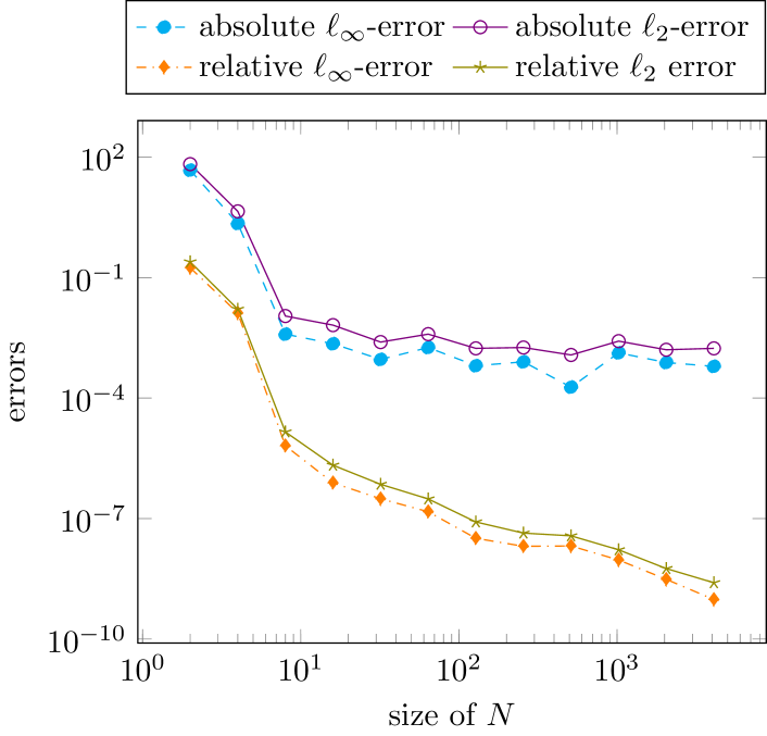
(a) $N=2^{c},\,c=1,\dots,12,$
$M=4N$ and  $m=4$.

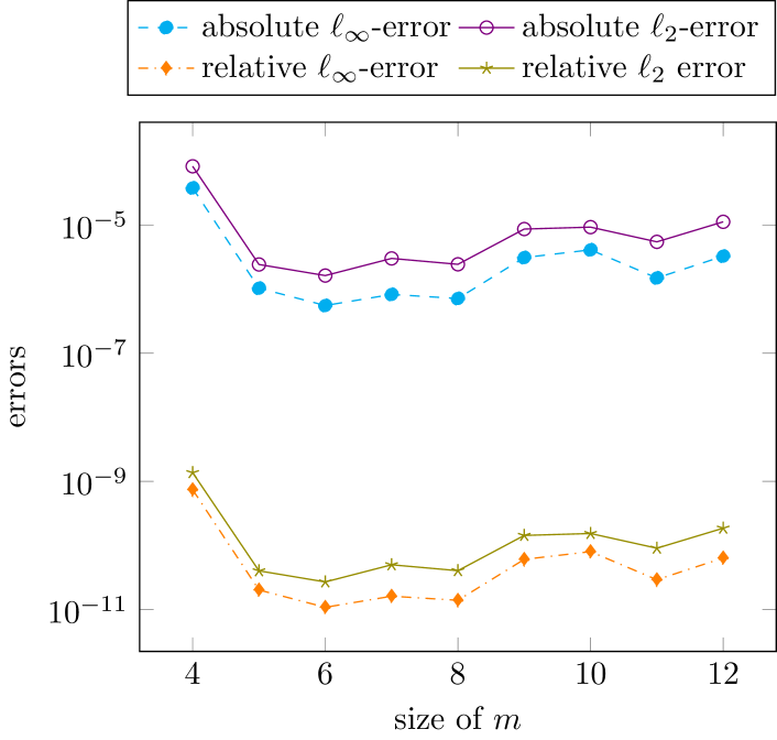
(b) $N=512,M=2048$
and $m=4,\dots,12$.

Figure 3.6: Comparison of the errors per node (3.25) of reconstructed Fourier coefficients generated by Algorithm 3.10 using the Dirichlet kernel and $\sigma=2.0$ for jittered equispaced nodes.

      

Remark 3.15.

The second problem (3.2) can be solved similarly by searching an approximation of the form $\boldsymbol{B}\boldsymbol{K}^{*}=\boldsymbol{B}\boldsymbol{F}\boldsymbol{D}\boldsymbol{A}^{*}\approx M\boldsymbol{I}_{N}$. Therefore, we consider the optimization problem

$$\underset{\boldsymbol{B}\in\mathbb{R}^{N\times M_{\sigma}}\colon\boldsymbol{B}\,(2m+1)\text{-sparse }}{\text{Minimize }}\ \|\boldsymbol{B}\boldsymbol{K}^{*}-M\boldsymbol{I}_{N}\|_{\textrm{F}}^{2}.$$

This is equivalent to the transposed problem

$$\underset{\boldsymbol{B}\in\mathbb{R}^{N\times M_{\sigma}}\colon\boldsymbol{B}\,(2m+1)\text{-sparse }}{\text{Minimize }}\ \|\boldsymbol{K}\boldsymbol{B}^{*}-M\boldsymbol{I}_{N}\|_{\textrm{F}}^{2},$$

which is what we discussed in Section 3.2.1 and hence can be solved likewise.       

Example 3.16.

Finally, we discuss the analogs of the examples mentioned above for problem (3.2). Since it is clear that the optimization problems are equivalent we refer to Example 3.13 for results with respect to the minimization of the norm. Similarly to Example 3.14, we check if we are able to perform an inverse adjoint NFFT for a trigonometric polynomial (1.1). This time we consider the estimate $\boldsymbol{\tilde{f}}=\left(\tilde{f}_{j}\right)_{j=1}^{N}=\frac{1}{M}\,\boldsymbol{B}_{\mathrm{opt}}\boldsymbol{F}\boldsymbol{D}(\boldsymbol{A}^{*}\boldsymbol{f})$ of the function values $\boldsymbol{f}=\left(f(x_{j})\right)_{j=1}^{N}=\left(f_{j}\right)_{j=1}^{N}$, where $\boldsymbol{B}_{\mathrm{opt}}$ is the adjoint of the output of Algorithm 3.10. We consider the absolute and relative errors per node

$$\frac{e_{r}^{\mathrm{abs}}}{N}=\frac{1}{N}\|\boldsymbol{\tilde{f}}-\boldsymbol{f}\|_{r}\quad\text{ and }\quad\frac{e_{r}^{\mathrm{rel}}}{N}=\frac{\|\boldsymbol{\tilde{f}}-\boldsymbol{f}\|_{r}}{N\,\|\boldsymbol{f}\|_{r}}$$ (3.26)

for $r\in\{2,\infty\}$ and perform the same experiments as in Example 3.14. The corresponding results can be found in Figure 3.7. There we see quite the same behavior in (a), whereas in (b) the errors get even worse when increasing the cut-off parameter $m$.

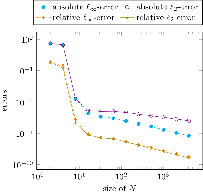
(a) $N=2^{c},\,c=1,\dots,12,$
$M=4N$ and  $m=4$.

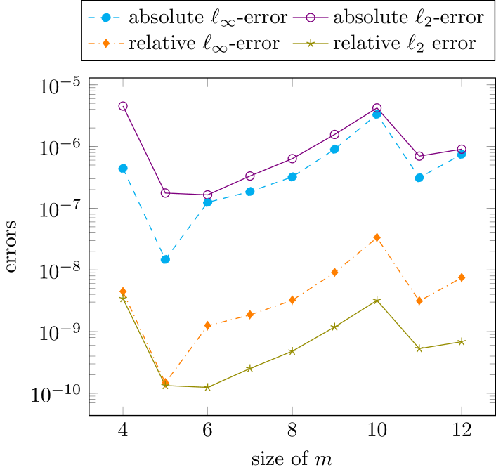
(b) $N=512,M=2048$
and $m=4,\dots,12$.

Figure 3.7: Comparison of the errors per node (3.9) of reconstructed function values generated by Algorithm 3.10 using the Dirichlet kernel and $\sigma=2.0$ for jittered equispaced nodes.

      

3.2.2 Inverse NFFT – overdetermined case

Previously, in Section 3.2.1 we studied $\boldsymbol{K}\boldsymbol{B}^{*}$ and $\boldsymbol{B}\boldsymbol{K}^{*}$, where $\boldsymbol{K}=\boldsymbol{A}\boldsymbol{D}^{*}\boldsymbol{F}^{*}\in\mathbb{C}^{N\times M_{\sigma}}$ and $\boldsymbol{B}\in\mathbb{R}^{N\times M_{\sigma}}$​. There we have seen that the inversion based on the minimization related to these matrices works best for $M>N$, which is the underdetermined case for the inverse NFFT as well as the overdetermined case for the inverse adjoint NFFT. However, often we are given nonequispaced samples with $M<N$ and search a corresponding trigonometric polynomial of degree $M$. Hence, we look for another approach which yields the best results in this overdetermined setting $M<N$. To this end, we investigate $\boldsymbol{B}^{*}\boldsymbol{K}$.

Initially, we consider the function $\tilde{g}(x)=\sum_{j=1}^{N}f_{j}\,\tilde{w}_{m}(x_{j}-x)$. Using this we can represent the vector $\tilde{\boldsymbol{g}}\coloneqq\left(\tilde{g}\left(\tfrac{l}{M_{\sigma}}\right)\right)_{l=-\frac{M_{\sigma}}{2}}^{\frac{M_{\sigma}}{2}-1}$ by $\tilde{\boldsymbol{g}}=\boldsymbol{B}^{*}\boldsymbol{f}$. Furthermore, we know by (2.8) that the adjoint NFFT can be written as $(\tilde{h}_{k})_{k=-\frac{M}{2}}^{\frac{M}{2}-1}\eqqcolon\tilde{\boldsymbol{h}}=\boldsymbol{D}^{*}\boldsymbol{F}^{*}\boldsymbol{B}^{*}\boldsymbol{f}$ and thereby we have $\tilde{\boldsymbol{h}}=\boldsymbol{D}^{*}\boldsymbol{F}^{*}\tilde{\boldsymbol{g}}$. Now we claim $\tilde{\boldsymbol{h}}\overset{!}{\approx}\boldsymbol{\hat{f}}$. Thus, it follows

$$\tilde{\boldsymbol{g}}=\boldsymbol{B}^{*}\boldsymbol{f}=\boldsymbol{B}^{*}\boldsymbol{A}\boldsymbol{\hat{f}}\overset{!}{\approx}\boldsymbol{B}^{*}\boldsymbol{A}\tilde{\boldsymbol{h}}=\boldsymbol{B}^{*}\boldsymbol{A}\boldsymbol{D}^{*}\boldsymbol{F}^{*}\tilde{\boldsymbol{g}}=\boldsymbol{B}^{*}\boldsymbol{K}\tilde{\boldsymbol{g}},$$

i. e., we seek $\boldsymbol{B}^{*}$ as the solution of the optimization problem

$$\underset{\boldsymbol{B}\in\mathbb{R}^{N\times M_{\sigma}}\colon\boldsymbol{B}\,(2m+1)\text{-sparse }}{\text{Minimize }}\ \left\|\boldsymbol{B}^{*}\boldsymbol{K}-\boldsymbol{I}_{M_{\sigma}}\right\|_{\mathrm{F}}^{2}.$$

This is equivalent to the transposed problem

$$\underset{\boldsymbol{B}\in\mathbb{R}^{N\times M_{\sigma}}\colon\boldsymbol{B}\,(2m+1)\text{-sparse }}{\text{Minimize }}\ \left\|\boldsymbol{K}^{*}\boldsymbol{B}-\boldsymbol{I}_{M_{\sigma}}\right\|_{\mathrm{F}}^{2}.$$ (3.27)

By means of definitions (3.14) and (2.6) we obtain

$$\boldsymbol{K}^{*}\boldsymbol{B}=\boldsymbol{F}\boldsymbol{D}\boldsymbol{A}^{*}\boldsymbol{B}=\left[\sum_{j=1}^{N}\sum_{k=-\frac{M}{2}}^{\frac{M}{2}-1}\frac{1}{M_{\sigma}\hat{w}(k)}\,\mathrm{e}^{-2\pi\mathrm{i}k\left(x_{j}-\frac{s}{M_{\sigma}}\right)}\,\tilde{w}_{m}\left(x_{j}-\tfrac{l}{M_{\sigma}}\right)\right]_{s,\,l=-\frac{M_{\sigma}}{2}}^{\frac{M_{\sigma}}{2}-1}.$$ (3.28)

Analogously to (3.16), we define the set

$$I_{M_{\sigma},m}(l):=\left\{j\in\left\{1,\dots,N\right\}:\exists\,z\in\mathbb{Z}\ \text{with}-m\leq M_{\sigma}x_{j}-l+M_{\sigma}z\leq m\right\}.$$ (3.29)

Hence, we can rewrite (3.27) by analogy with Section 3.2.1 as

$$\left\|\boldsymbol{F}\boldsymbol{D}\boldsymbol{A}^{*}\boldsymbol{B}-\boldsymbol{I}_{M_{\sigma}}\right\|_{\mathrm{F}}^{2}=\sum_{l=-\frac{M_{\sigma}}{2}}^{\frac{M_{\sigma}}{2}-1}\|\boldsymbol{F}\boldsymbol{D}\boldsymbol{H}_{l}\boldsymbol{b}_{l}-\boldsymbol{e}_{l}\|_{2}^{2},$$

where

$$\boldsymbol{b}_{l}\coloneqq\bigg{(}\tilde{w}_{m}\left(x_{j}-\tfrac{l}{M_{\sigma}}\right)\bigg{)}_{j\in I_{M_{\sigma},m}(l)},\quad\boldsymbol{H}_{l}\coloneqq\left(\mathrm{e}^{-2\pi\mathrm{i}kx_{j}}\right)_{k=-\frac{M}{2},\,j\in I_{M_{\sigma},m}(l)}^{\frac{M}{2}-1}$$

and $\boldsymbol{e}_{l}$ denote the columns of the identity matrix $\boldsymbol{I}_{M_{\sigma}}$. We obtain, cf. (3.20),

$$\boldsymbol{L}_{l}\coloneqq\boldsymbol{F}\boldsymbol{D}\boldsymbol{H}_{l}=\left[\frac{1}{M_{\sigma}}\sum_{k=-\frac{M}{2}}^{\frac{M}{2}-1}\frac{1}{\hat{w}(k)}\,\mathrm{e}^{2\pi\mathrm{i}k\left(\frac{s}{M_{\sigma}}-x_{j}\right)}\right]_{s=-\frac{M_{\sigma}}{2},\,j\in I_{M_{\sigma},m}(l)}^{\frac{M_{\sigma}}{2}-1}\in\mathbb{C}^{M_{\sigma}\times|I_{M_{\sigma},m}(l)|}.$$ (3.30)

Thereby we receive the optimization problems

$$\underset{\tilde{\boldsymbol{b}}_{l}\in\mathbb{R}^{2m+1}}{\text{Minimize }}\ \|\boldsymbol{L}_{l}\tilde{\boldsymbol{b}}_{l}-\boldsymbol{e}_{l}\|_{2}^{2},\quad l=-\tfrac{M_{\sigma}}{2},\dots,\tfrac{M_{\sigma}}{2}-1.$$

If the matrix $\boldsymbol{L}_{l}\in\mathbb{C}^{M_{\sigma}\times|I_{M_{\sigma},m}(l)|}$ has full rank the solution of (3.27) is given by

$$\tilde{\boldsymbol{b}}_{l}=\left(\boldsymbol{L}_{l}^{*}\boldsymbol{L}_{l}\right)^{-1}\boldsymbol{L}_{l}^{*}\boldsymbol{e}_{l},\quad l=-\tfrac{M_{\sigma}}{2},\dots,\tfrac{M_{\sigma}}{2}-1.$$ (3.31)

This time we cannot tell anything about the dimensions of $\boldsymbol{L}_{l}$ in general since the size of the set $I_{M_{\sigma},m}(l)$ depends on several parameters. Having these vectors $\tilde{\boldsymbol{b}}_{l}$ we can compose the modified matrix $\boldsymbol{B}_{\mathrm{opt}}$, observing that $\tilde{\boldsymbol{b}}_{l}$ only consist of the nonzero entries of $\boldsymbol{B}_{\mathrm{opt}}$. Then the approximation of the Fourier coefficients is given by

$$\boldsymbol{\hat{f}}\approx\tilde{\boldsymbol{h}}=\boldsymbol{D}^{*}\boldsymbol{F}^{*}\boldsymbol{B}_{\mathrm{opt}}^{*}\boldsymbol{f}.$$ (3.32)

In other words, this approach yields another way to invert the NFFT by also modifying the adjoint NFFT.

Analogously to Section 3.2.1, we are able to compute the entries of the matrix $\boldsymbol{L}_{l}$, see (3.30), by means of an NFFT with the $M$ coefficients

$$\hat{f}_{k}=\frac{1}{M_{\sigma}\hat{w}(k)},\quad k=-\tfrac{M}{2},\dots,\tfrac{M}{2}-1,$$ (3.33)

and nodes $y_{s,j}\coloneqq\tfrac{s}{M_{\sigma}}-x_{j},\,s=-\tfrac{M_{\sigma}}{2},\dots,\tfrac{M_{\sigma}}{2}-1,\,j\in I_{M_{\sigma},m}(l),$ which are at most $M_{\sigma}N$ many. Here we also require only one NFFT by writing the columns of $\boldsymbol{L}_{l}$ one below the other. The obtained vector including all entries of $\boldsymbol{L}_{l}$ has to be reshaped afterwards. This leads to the following algorithm.

Algorithm 3.17 (Fast optimization of the matrix $\boldsymbol{B}$).

  
For $N\in\mathbb{N}$ let $x_{j}\in\left[-\frac{1}{2},\frac{1}{2}\right),j=1,\dots,N,$ be given nodes as well as $M\in 2\mathbb{N}$, $\sigma\geq 1$ and $M_{\sigma}=\sigma M$.

1. Compute $\boldsymbol{g}=\boldsymbol{F}\boldsymbol{D}\boldsymbol{\hat{f}}$, cf. (2.4) and (2.5), with $\hat{f}_{k}$ in (3.33). $\mathcal{O}(M\log M)$

2. For $l=-\frac{M_{\sigma}}{2},\dots,\frac{M_{\sigma}}{2}-1$:

   • Determine the set $I_{M_{\sigma},m}(l)$, cf. (3.29). $\mathcal{O}(N)$

   • Perform $\boldsymbol{B}\boldsymbol{g}$, cf. (2.6), for the vector of nodes

     $$\boldsymbol{y}\coloneqq\left(\boldsymbol{y}_{1}^{T},\dots,\boldsymbol{y}_{s}^{T}\right)^{T}$$

     for $\boldsymbol{y}_{n}$ being the columns of the matrix $\boldsymbol{Y}\coloneqq(y_{l,j})_{l=-\frac{M_{\sigma}}{2},\,j\in I_{M_{\sigma},m}(l)}^{\frac{M_{\sigma}}{2}-1}$. $\mathcal{O}(N)$

   • Reshape the obtained vector into the matrix $\boldsymbol{L}_{l}\in\mathbb{C}^{M_{\sigma}\times|I_{M_{\sigma},m}(l)|}$. $\mathcal{O}(N)$

   • Solve the normal equations for $\boldsymbol{L}_{l}$, cf. (3.31). $\mathcal{O}(N^{3}+N^{2}M)$

3. Compose $\boldsymbol{B}_{\mathrm{opt}}$ column-wise of the vectors $\tilde{\boldsymbol{b}}_{l}$ observing the periodicity. $\mathcal{O}(M)$

Output: optimized matrix $\boldsymbol{B}_{\mathrm{opt}}$
Complexity: $\mathcal{O}(N^{2}M^{2}+N^{3}M)$  
 

Remark 3.18.

If we assume the nodes are somewhat uniformly distributed, like for instance jittered equispaced nodes, we can get rid of the complexity related to $N$ and end up with arithmetic costs of $\mathcal{O}(M^{2})$.       

Remark 3.19.

It is also possible to simplify the computation of $\boldsymbol{L}_{l}$ by incorporating the Dirichlet kernel (3.23), i. e., we set $\hat{w}(k)=1$ for all $k=-\frac{M}{2}+1,\dots,\frac{M}{2}-1,$ and the last nonzero entry $\frac{1}{\hat{w}(\frac{M}{2})}$ of the matrix $\boldsymbol{D}^{*}$ is set to zero. Hence, the entries of the matrix

$$\boldsymbol{L}_{l}=\left[\frac{1}{M_{\sigma}}\,D_{\frac{M}{2}-1}\left(\tfrac{l}{M_{\sigma}}-x_{j}\right)\right]_{l=-\frac{M_{\sigma}}{2},\,j\in I_{M_{\sigma},m}(l)}^{\frac{M_{\sigma}}{2}-1}$$

can explicitly be stated and therefore the term $M\log M$ in the computational costs of Algorithm 3.17 can be eliminated. Nevertheless, even if we assume uniformly distributed nodes as in Remark 3.18, we remain with arithmetic costs of $\mathcal{O}(M^{2})$.       

Remark 3.20.

This algorithm using a window function or the Dirichlet kernel is part of the software package NFFT 3.5.1, see [19, ./matlab/infft1d].       

Example 3.21.

As in Example 3.13 we verify at first that the optimization was successful. On that account, we compare the norms

$$\left\|\boldsymbol{F}\boldsymbol{D}\boldsymbol{A}^{*}\boldsymbol{B}-\boldsymbol{I}_{M_{\sigma}}\right\|_{\mathrm{F}}\quad\text{ and }\quad\|\boldsymbol{F}\boldsymbol{D}\boldsymbol{A}^{*}\boldsymbol{B}_{\mathrm{opt}}-\boldsymbol{I}_{M_{\sigma}}\|_{\mathrm{F}},$$ (3.34)

where $\boldsymbol{B}$ denotes the original matrix from the NFFT and $\boldsymbol{B}_{\mathrm{opt}}$ the optimized matrix generated by Algorithm 3.17. Although our method is attributed to the overdetermined setting, this again means no restriction. Therefore, also the underdetermined setting is tested.

• Again we examine at first jittered equispaced nodes, see (3.8). We choose $M=128$ and consider the norms (3.34) for $N=2^{c}$ nodes with $c=2,\dots,14$. In order to compute the NFFT in Algorithm 3.17 we choose the Kaiser-Bessel window, an oversampling of $\sigma_{2}=2.0$ and the cut-off parameter $m_{2}=2m$ to achieve results comparable to Example 3.13. However, one could also choose a larger cut-off to receive more accuracy for growing $N$.

  In Figure 3.8 one can find the comparison of the norms (3.34) for different values of $m$ and $\sigma$ for $\boldsymbol{B}_{\mathrm{opt}}$ generated using B-Splines as well as the Dirichlet kernel mentioned in Remark 3.19. It can be seen that for $\sigma=1.0$ the minimization was very successful especially for large $N$ compared to $M$. For $N<M$ the minimization was not successful. Similarly to Example 3.13, this results from the fact that the corresponding matrix $\boldsymbol{F}\boldsymbol{D}\boldsymbol{A}^{*}\boldsymbol{B}$ is of low rank. Therefore, Algorithm 3.17 is specially attributed to the overdetermined case.

  Having a look at the graphs with high oversampling we recognize that the norms of the optimized matrices remain stable for all sizes of $N$. Thus, also for this method the optimization seems not to work for high oversampling.

  While the computational costs could not be scaled down, we see in Figure 3.9 that using the Dirichlet kernel reduced the run-time for all sizes of $N$. Results for other window functions are omitted since they show the same behavior.

• Next we repeat the example using Chebyshev nodes, cf. (3.10). The corresponding results for B-Splines can be found in Figure 3.10. We recognize that these graphs look similar to Figure 3.8, in contrast to Example 3.13 where the optimization for Chebyshev nodes was quite difficult.       

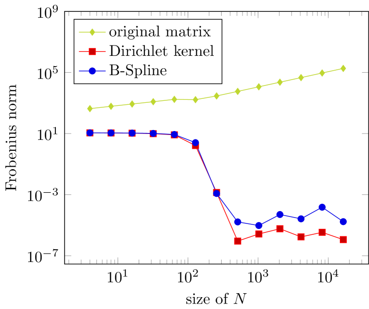
(a) $m=2$ and $\sigma=1.0$

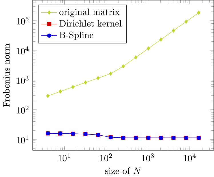
(b) $m=2$ and $\sigma=2.0$

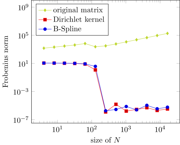
(c) $m=4$ and $\sigma=1.0$

Figure 3.8: Comparison of Frobenius norms (3.34) of the original matrix $\boldsymbol{B}$ and the optimized matrix $\boldsymbol{B}_{\mathrm{opt}}$ generated by Algorithm 3.17 using B-Spline window functions as well as the Dirichlet kernel for $M=128$ and $N=2^{c}$ jittered equispaced nodes with $c=2,\dots,14$.

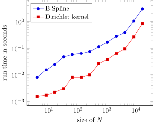
Figure 3.9: Comparison of run-times of Algorithm 3.17 using the B-Spline as well as the Dirichlet kernel with $m=2$ and $\sigma=1.0$ for $M=128$ and $N=2^{c}$ jittered equispaced nodes with $c=2,\dots,14$.

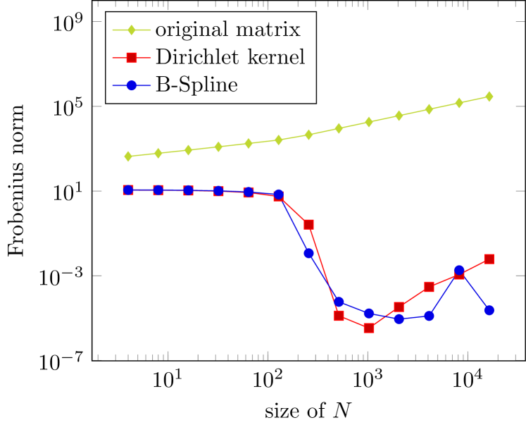
(a) $m=2$ and $\sigma=1.0$

(b) $m=2$ and $\sigma=2.0$

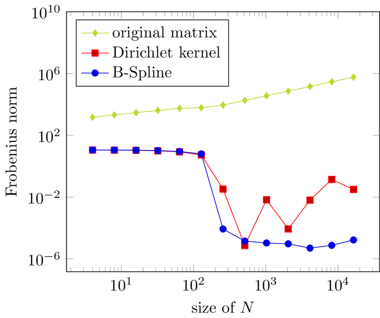
(c) $m=4$ and $\sigma=1.0$

Figure 3.10: Comparison of Frobenius norms (3.34) of the original matrix $\boldsymbol{B}$ and the optimized matrix $\boldsymbol{B}_{\mathrm{opt}}$ generated by Algorithm 3.17 using B-Spline window functions as well as the Dirichlet kernel for $M=128$ and $N=2^{c}$ Chebyshev nodes with $c=2,\dots,14$.

Remark 3.22.

Another approach for computing an inverse NFFT in the setting $N\geq M$ can be obtained by using the fact that $\boldsymbol{A}^{*}\boldsymbol{A}$ is of Toeplitz structure. To this end, the Gohberg-Semencul formula, see [18], can be used to solve the normal equations $\boldsymbol{A}^{*}\boldsymbol{A}\boldsymbol{\hat{f}}=\boldsymbol{A}^{*}\boldsymbol{f}$ exactly by analogy with [3]. Therefore, the inverse NFFT consists of two steps: an adjoint NFFT applied to $\boldsymbol{f}$ and the multiplication with the inverse of $\boldsymbol{A}^{*}\boldsymbol{A}$, which can be realized by means of 8 FFTs. The computation of the components of the Gohberg-Semencul formula can be seen as a precomputational step.

However, even if this algorithm is exact and therefore yields better results than our approach from Section 3.2.2 there is no exact generalization to higher dimensions since there is no generalization of the Gohberg-Semencul formula to dimensions $>1$. This approach can only be used for approximations on very special grids, such as linogramm grids, utilizing the given specific structure, see [2, 3].       

Example 3.23.

As in Example 3.14 we consider a trigonometric polynomial. For $\boldsymbol{f}=\left(f(x_{j})\right)_{j=1}^{N}$ with given nodes $x_{j}$ we consider the estimate $\boldsymbol{\check{f}}=\left(\check{f}_{k}\right)_{k=-\frac{M}{2}}^{\frac{M}{2}-1}=\boldsymbol{D}^{*}\boldsymbol{F}^{*}\boldsymbol{B}_{\mathrm{opt}}^{*}\boldsymbol{f}$, where $\boldsymbol{B}_{\mathrm{opt}}^{*}$ is the outcome of Algorithm 3.17, and compare it to the given function values $\boldsymbol{f}$. Again, we choose the Dirichlet kernel with $\sigma=2.0$ and jittered equispaced nodes $x_{j}$. We consider the absolute and relative errors per node (3.9) for $r\in\{2,\infty\}$. As a first experiment we use $M=2^{c}$ with $c=1,\dots,12$, $N=4M$, and $m=4$. In a second experiment we fix $N=2048$ and $M=512$ and the cut-off parameter $m$ shall be chosen $m=c$ with $c=4,\dots,12$. The corresponding results are displayed in Figure 3.11. We recognize that the errors per node for growing $M$, see (a), are worse if we consider very small sizes of $N$ but decrease for large sizes of $M$. In (b) we can see that for fixed $M$ these errors remain quite stable when tuning the cut-off parameter $m$. One could also consider the Toeplitz approach described in Remark 3.22. There we observed stable absolute errors of size $10^{-15}$ and stable relative errors of size $10^{-18}$.

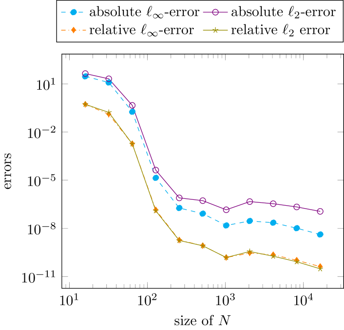
(a) $M=2^{c},\,c=1,\dots,12,$
$N=4M$ and  $m=4$.

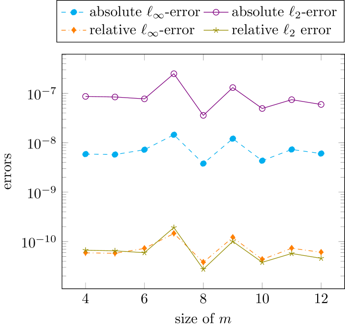
(b) $N=2048,M=512$
and $m=4,\dots,12$.

Figure 3.11: Comparison of the errors per node (3.9) of reconstructed Fourier coefficients generated by Algorithm 3.17 using the Dirichlet kernel and $\sigma=2.0$ for jittered equispaced nodes.

      

Remark 3.24.

Having a look at the remaining matrix product $\boldsymbol{K}^{*}\boldsymbol{B}$ we recognize that the corresponding optimization problem

$$\underset{\boldsymbol{B}\in\mathbb{R}^{N\times M_{\sigma}}\colon\boldsymbol{B}\,(2m+1)\text{-sparse }}{\text{Minimize }}\ \left\|\boldsymbol{K}^{*}\boldsymbol{B}-\boldsymbol{I}_{M_{\sigma}}\right\|_{\mathrm{F}}^{2}$$

was already solved to find a solution for the transposed problem

$$\underset{\boldsymbol{B}\in\mathbb{R}^{N\times M_{\sigma}}\colon\boldsymbol{B}\,(2m+1)\text{-sparse }}{\text{Minimize }}\ \left\|\boldsymbol{B}^{*}\boldsymbol{K}-\boldsymbol{I}_{M_{\sigma}}\right\|_{\mathrm{F}}^{2}.$$

Hence, it is merely left to examine the current approximation. Due to the minimization problem we have $\boldsymbol{F}\boldsymbol{D}\boldsymbol{A}^{*}\boldsymbol{B}=\boldsymbol{K}^{*}\boldsymbol{B}\approx\boldsymbol{I}_{M_{\sigma}}$. Because $\boldsymbol{B}\in\mathbb{R}^{N\times M_{\sigma}}$ is rectangular and therefore not invertible we multiply by a right-inverse of $\boldsymbol{B}$, i. e., a matrix $\boldsymbol{B}^{\prime}\in\mathbb{R}^{M_{\sigma}\times N}$ that holds $\boldsymbol{B}\boldsymbol{B}^{\prime}=\boldsymbol{I}_{N}$, and receive $\boldsymbol{F}\boldsymbol{D}\boldsymbol{A}^{*}\approx\boldsymbol{B}^{\prime}$. Multiplying by a vector $\boldsymbol{f}$ yields $\boldsymbol{F}\boldsymbol{D}\boldsymbol{A}^{*}\boldsymbol{f}\approx\boldsymbol{B}^{\prime}\boldsymbol{f}$, which can be written by means of $\boldsymbol{A}^{*}\boldsymbol{f}=\boldsymbol{h}$ as $\boldsymbol{F}\boldsymbol{D}\boldsymbol{h}\approx\boldsymbol{B}^{\prime}\boldsymbol{f}$. Finally, we multiply left-hand by $\boldsymbol{B}$, which results in the approximation $\boldsymbol{B}\boldsymbol{F}\boldsymbol{D}\boldsymbol{h}\approx\boldsymbol{f}$ and thus provides another method to invert the adjoint NFFT by modifying the NFFT.       

Example 3.25.

Finally, we consider the analog of Example 3.16. To this end, we exchange the estimate by $\boldsymbol{\tilde{f}}=\boldsymbol{B}_{\mathrm{opt}}\boldsymbol{F}\boldsymbol{D}(\boldsymbol{A}^{*}\boldsymbol{f})$, where $\boldsymbol{B}_{\mathrm{opt}}$ is the adjoint of the outcome of Algorithm 3.17. We conduct the same experiments as in Example 3.23 but consider the errors per node (3.26). The corresponding results can be found in Figure 3.12. There we see that our optimization was not successful in the case $N>M$ since there is no reasonable chance to approximate the function values in any of the tested settings.

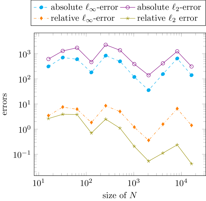
(a) $M=2^{c},\,c=1,\dots,12,$
$N=4M$ and  $m=4$.

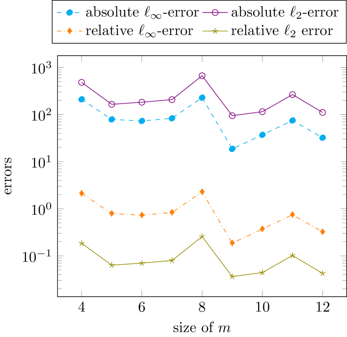
(b) $N=2048,M=512$
and $m=4,\dots,12$.

Figure 3.12: Comparison of the errors per node (3.9) of reconstructed function values generated by Algorithm 3.17 using the Dirichlet kernel and $\sigma=2.0$ for jittered equispaced nodes.

      

4 Frames

During the last few decades the popularity of frames rose rapidly and more and more articles are concerned with this topic. Recently, an approach was published in [15] connecting frame approximation to the adjoint NFFT. Thus, in this section we consider the concept of frames and discuss an approach for inverting the NFFT based on [15]. Besides the basic information about the approximation of the inverse frame operator, a link to the methods explained in Section 3.2 is provided.

4.1 Approximation of the inverse frame operator

First of all, we sum up the main idea of frames and frame approximation, basically adapted from [15] and [7].

Definition 4.1.

Let $\mathcal{H}$ be a separable Hilbert space with inner product $\langle\cdot,\cdot\rangle$. Then a sequence $\{\varphi_{j}\}_{j=1}^{\infty}\subset\mathcal{H}$ is called frame if there exist constants $A,B>0$ such that

$$A\|f\|^{2}\leq\sum_{j=1}^{\infty}|\langle f,\varphi_{j}\rangle|^{2}\leq B\|f\|^{2}\quad\forall f\in\mathcal{H}.$$

The operator $S\colon\mathcal{H}\to\mathcal{H},Sf=\sum_{j=1}^{\infty}\langle f,\varphi_{j}\rangle\varphi_{j}$, is named the frame operator.       

Given this definition we can already state one of the most important results in frame theory, the so-called frame decomposition. If $\{\varphi_{j}\}_{j=1}^{\infty}$ is a frame with frame operator $S$, then

$$f=\sum_{j=1}^{\infty}\langle f,S^{-1}\varphi_{j}\rangle\varphi_{j}=\sum_{j=1}^{\infty}\langle f,\varphi_{j}\rangle S^{-1}\varphi_{j}\quad\forall f\in\mathcal{H}.$$ (4.1)

In other words, every element of $\mathcal{H}$ can be represented as a linear combination of the elements of the frame, which is a property similar to an orthonormal basis. Though, to apply (4.1) it is necessary to state the inverse operator $S^{-1}$ explicitly. However, this is usually difficult (or even impossible). Hence, it is necessary to be able to approximate $S^{-1}$. For this purpose, we use the method from [14] by analogy with [15], which is based on so-called admissible frames, see [15, Definition 1].

We suppose $\{\psi_{l}\}_{l=-\infty}^{\infty}$ is an admissible frame with respect to $\{\varphi_{j}\}_{j=1}^{\infty}$. As shown in [14], the dual frame $\{S^{-1}\varphi_{j}\}_{j=1}^{\infty}$ can then be approximated by

$$S^{-1}\varphi_{j}\approx\tilde{\varphi}_{j}\coloneqq\sum_{l=-\frac{M_{\sigma}}{2}}^{\frac{M_{\sigma}}{2}-1}p_{l,j}\,\psi_{l},\quad j=1,\dots,N,$$ (4.2)

where $\boldsymbol{\Phi}^{\dagger}\eqqcolon\left[p_{l,j}\right]_{l=-\frac{M_{\sigma}}{2},\,j=1}^{\frac{M_{\sigma}}{2}-1,\;N}$ is the Moore-Penrose pseudoinverse of the matrix

$$\boldsymbol{\Phi}\coloneqq\left[\langle\varphi_{j},\psi_{l}\rangle\right]_{j=1,\,l=-\frac{M_{\sigma}}{2}}^{N,\ \frac{M_{\sigma}}{2}-1}.$$ (4.3)

In so doing, the matrix dimensions have to fulfill the condition $N\geq M_{\sigma}+cM_{\sigma}^{\frac{1}{2s-1}}$. Given this approximation of the dual frame, inserting (4.2) in (4.1) and cutting off the infinite sum yields the approximation

$$f\approx\tilde{f}\coloneqq\sum_{j=1}^{N}\sum_{l=-\frac{M_{\sigma}}{2}}^{\frac{M_{\sigma}}{2}-1}\langle f,\varphi_{j}\rangle\,p_{l,j}\,\psi_{l}.$$ (4.4)

4.2 Linking the frame-theoretical approach to the iNFFT

Now we aim to find a link between the frame approximation (4.4) and the iNFFT from Section 3.2. To this end, we consider a discrete version of the frames recommended in [15], i. e.,

$$\{\varphi_{j}(k)\coloneqq\mathrm{e}^{-2\pi\mathrm{i}kx_{j}},\,j\in\mathbb{N}\}\quad\text{ and }\quad\left\{\psi_{l}(k)\coloneqq\frac{\mathrm{e}^{-2\pi\mathrm{i}kl/M_{\sigma}}}{M_{\sigma}\hat{w}(-k)},\,l\in\mathbb{Z}\right\}$$ (4.5)

for $k\in\mathbb{Z}$, where $x_{j}\in[-\frac{1}{2},\frac{1}{2})$ denote the nonequispaced nodes. Note that we changed time and frequency domain to match our notations in Section 2. Thereby, we receive the scalar product

$$\langle\varphi_{j},\psi_{l}\rangle_{\ell_{2}}=\sum_{k=-\infty}^{\infty}\varphi_{j}(k)\,\overline{\psi_{l}(k)}=\sum_{k=-\infty}^{\infty}\frac{1}{M_{\sigma}\hat{w}(k)}\,\mathrm{e}^{-2\pi\mathrm{i}k\left(x_{j}-\frac{l}{M_{\sigma}}\right)}.$$

Truncating the infinite sum yields an approximation of the matrix $\boldsymbol{\Phi}$ in (4.3) by

$$\boldsymbol{\Phi}_{\ell_{2}}=\bigg{(}\overline{K\left(x_{j}-\tfrac{l}{M_{\sigma}}\right)}\bigg{)}_{j=1,\,l=-\frac{M_{\sigma}}{2}}^{N,\ \frac{M_{\sigma}}{2}-1}$$ (4.6)

with the kernel $K(x)$ from (3.15). In the following explanations we choose $\boldsymbol{\Phi}=\boldsymbol{\Phi}_{\ell_{2}}$.

Remark 4.2.

In general, we do not have admissible frames for our known window functions $w$ because of the factor $\frac{1}{\hat{w}(k)}$, $k=-\infty,\dots,\infty$. Only for finite frames the appropriate conditions can be satisfied. In addition, it must be pointed out that for other sampling patterns than the jittered equispaced nodes it was already mentioned in [8] that the admissibility condition may not hold or even the conditions for constituting a frame may fail, cf. [15].       

4.2.1 Theoretical results

For these given frames we consider again the frame approximation (4.4). Our aim is to show that the inversion of the NFFT illustrated in Section 3.2 can also be expressed by means of a frame-theoretical approach, i. e., by approximating a function $\hat{f}$ in the frequency domain, cf. (2.3), and subsequently sampling at equispaced points $k=-\frac{M}{2},\dots,\frac{M}{2}-1$.

The frame approximation of the function $\hat{f}$ is given by

$$\tilde{\hat{f}}=\sum_{j=1}^{N}\sum_{l=-\frac{M_{\sigma}}{2}}^{\frac{M_{\sigma}}{2}-1}\langle\hat{f},\varphi_{j}\rangle_{\ell_{2}}\,p_{l,j}\,\psi_{l}$$ (4.7)

with $p_{l,j}$ as defined in (4.2). Hence, we are acquainted with two different methods to compute the Fourier coefficients $\hat{f}_{k}$ from given data $\langle\hat{f},\varphi_{j}\rangle\eqqcolon f_{j}$, the frame approximation (4.7) as well as the adjoint NFFT (2.8). In what follows, we suppose that we can achieve a reconstruction via frames. Utilizing this, we modify the adjoint NFFT so that we can use this simple method to invert the NFFT. Thus, we are looking for an approximation of the form $\tilde{h}_{k}\approx\tilde{\hat{f}}(k)\approx\hat{f}_{k}$,  $k=-\tfrac{M}{2},\dots,\tfrac{M}{2}-1$.

To compare the adjoint NFFT and the frame approximation we firstly rewrite the approximation (2.8) of the adjoint NFFT by analogy with [15]. This yields

$$\tilde{h}_{k}=\sum_{l=-\frac{M_{\sigma}}{2}}^{\frac{M_{\sigma}}{2}-1}c_{l}\,\psi_{l}(k),\quad k=-\tfrac{M}{2},\dots,\tfrac{M}{2}-1,$$ (4.8)

with coefficients vector

$$\boldsymbol{c}\coloneqq\left(c_{l}\right)_{l=-\frac{M_{\sigma}}{2}}^{\frac{M_{\sigma}}{2}-1}=\left(\sum_{j=1}^{N}f_{j}\,\tilde{w}_{m}\left(x_{j}-\tfrac{l}{M_{\sigma}}\right)\right)_{l=-\frac{M_{\sigma}}{2}}^{\frac{M_{\sigma}}{2}-1}=\boldsymbol{B}^{*}\boldsymbol{f},$$ (4.9)

where $\boldsymbol{f}\coloneqq\left(f_{j}\right)_{j=1}^{N}=(\langle\hat{f},\varphi_{j}\rangle_{\ell_{2}})_{j=1}^{N}.$ Likewise we rewrite (4.7), cf. [15], as

$$\tilde{\tilde{h}}_{k}\coloneqq\tilde{\hat{f}}(k)=\sum_{l=-\frac{M_{\sigma}}{2}}^{\frac{M_{\sigma}}{2}-1}d_{l}\,\psi_{l}(k),\quad k=-\tfrac{M}{2},\dots,\tfrac{M}{2}-1,$$ (4.10)

with $\boldsymbol{d}\coloneqq\left(d_{l}\right)_{l=-\frac{M_{\sigma}}{2}}^{\frac{M_{\sigma}}{2}-1}=\boldsymbol{\Phi}^{\dagger}\boldsymbol{f}.$ Furthermore, we define the vectors $\tilde{\boldsymbol{h}}\coloneqq(\tilde{h}_{k})_{k=-\frac{M}{2}}^{\frac{M}{2}-1}$ and $\tilde{\tilde{\boldsymbol{h}}}\coloneqq(\tilde{\tilde{h}}_{k})_{k=-\frac{M}{2}}^{\frac{M}{2}-1}$ as well as the matrix $\boldsymbol{\Psi}\coloneqq(\psi_{l}(k))_{k=-\frac{M}{2},\,l=-\frac{M_{\sigma}}{2}}^{\frac{M}{2}-1,\ \frac{M_{\sigma}}{2}-1}$. Thereby, (4.8) and (4.10) can be represented by $\tilde{\boldsymbol{h}}=\boldsymbol{\Psi}\boldsymbol{c}$ and $\tilde{\tilde{\boldsymbol{h}}}=\boldsymbol{\Psi}\boldsymbol{d}$. Hence, we can now estimate the difference between both approximations.

Theorem 4.3.

Let $\hat{\boldsymbol{w}}\coloneqq\left((\hat{w}(-k))^{-1}\right)_{k=-\frac{M}{2}}^{\frac{M}{2}-1}$ be a vector satisfying $\|\hat{\boldsymbol{w}}\|_{2}<\infty$. Then the following estimates hold.

1. For $M_{\sigma}<N$ we have

   $$\left\|\tilde{\boldsymbol{h}}-\tilde{\tilde{\boldsymbol{h}}}\right\|_{2}\leq\frac{1}{\sqrt{M_{\sigma}}}\left\|\hat{\boldsymbol{w}}\right\|_{2}\,\|\boldsymbol{\Phi}\boldsymbol{B}^{*}-\boldsymbol{I}_{N}\|_{\textrm{F}}\,\|\boldsymbol{\Phi}^{\dagger}\boldsymbol{f}\|_{2}.$$ (4.11)

2. For $M_{\sigma}>N$ we have

   $$\left\|\tilde{\boldsymbol{h}}-\tilde{\tilde{\boldsymbol{h}}}\right\|_{2}\leq\frac{1}{\sqrt{M_{\sigma}}}\left\|\hat{\boldsymbol{w}}\right\|_{2}\,\|\boldsymbol{B}^{*}\boldsymbol{\Phi}-\boldsymbol{I}_{M_{\sigma}}\|_{\textrm{F}}\,\|\boldsymbol{\Phi}^{\dagger}\boldsymbol{f}\|_{2},$$ (4.12)

where $\boldsymbol{B}^{*}$ denotes the adjoint matrix of (2.6) and $\boldsymbol{\Phi}=\boldsymbol{\Phi}_{\ell_{2}}$ is given as in (4.6).

Proof.

By analogy with [15] Definitions (4.8) and (4.10) imply

$$\begin{split}\left\|\tilde{\boldsymbol{h}}-\tilde{\tilde{\boldsymbol{h}}}\right\|_{2}=\left\|\boldsymbol{\Psi}\boldsymbol{c}-\boldsymbol{\Psi}\boldsymbol{d}\right\|_{2}\leq\left\|\boldsymbol{\Psi}\right\|_{\mathrm{F}}\left\|\boldsymbol{c}-\boldsymbol{d}\right\|_{2}=\sqrt{\sum_{k=-\frac{M}{2}}^{\frac{M}{2}-1}\sum_{l=-\frac{M_{\sigma}}{2}}^{\frac{M_{\sigma}}{2}-1}|\psi_{l}(k)|^{2}}\,\cdot\left\|\boldsymbol{c}-\boldsymbol{d}\right\|_{2}\\ =\frac{1}{M_{\sigma}}\sqrt{\sum_{k=-\frac{M}{2}}^{\frac{M}{2}-1}\left|\frac{1}{\hat{w}(-k)}\right|^{2}\sum_{l=-\frac{M_{\sigma}}{2}}^{\frac{M_{\sigma}}{2}-1}\underbrace{\left|\mathrm{e}^{-2\pi\mathrm{i}kl/M_{\sigma}}\right|^{2}}_{\leq 1}}\,\cdot\left\|\boldsymbol{c}-\boldsymbol{d}\right\|_{2}\leq\frac{1}{\sqrt{M_{\sigma}}}\left\|\hat{\boldsymbol{w}}\right\|_{2}\left\|\boldsymbol{c}-\boldsymbol{d}\right\|_{2}.\end{split}$$

Next we consider the norm $\|\boldsymbol{c}-\boldsymbol{d}\|_{2}$ separately.

1. For $M_{\sigma}<N$ we have by (4.9) and (4.10) that

   $$\boldsymbol{c}-\boldsymbol{d}=\big{(}\boldsymbol{B}^{*}-\boldsymbol{\Phi}^{\dagger}\big{)}\boldsymbol{f}=\big{(}\boldsymbol{B}^{*}-(\boldsymbol{\Phi}^{*}\boldsymbol{\Phi})^{-1}\boldsymbol{\Phi}^{*}\big{)}\boldsymbol{f}=\big{(}(\boldsymbol{\Phi}^{*}\boldsymbol{\Phi})^{-1}\boldsymbol{\Phi}^{*}\big{)}(\boldsymbol{\Phi}\boldsymbol{B}^{*}-\boldsymbol{I}_{N})\boldsymbol{f}.$$

   This leads to

   $$\|\boldsymbol{c}-\boldsymbol{d}\|_{2}\leq\|\boldsymbol{\Phi}\boldsymbol{B}^{*}-\boldsymbol{I}_{N}\|_{\textrm{F}}\,\|\big{(}(\boldsymbol{\Phi}^{*}\boldsymbol{\Phi})^{-1}\boldsymbol{\Phi}^{*}\big{)}\boldsymbol{f}\|_{2}\leq\|\boldsymbol{\Phi}\boldsymbol{B}^{*}-\boldsymbol{I}_{N}\|_{\textrm{F}}\,\|\boldsymbol{\Phi}^{\dagger}\boldsymbol{f}\|_{2}.$$

2. In analogy, for $M_{\sigma}>N$ we have that

   $$\boldsymbol{c}-\boldsymbol{d}=\big{(}\boldsymbol{B}^{*}-\boldsymbol{\Phi}^{\dagger}\big{)}\boldsymbol{f}=\big{(}\boldsymbol{B}^{*}-\boldsymbol{\Phi}^{*}(\boldsymbol{\Phi}\boldsymbol{\Phi}^{*})^{-1}\big{)}\boldsymbol{f}=(\boldsymbol{B}^{*}\boldsymbol{\Phi}-\boldsymbol{I}_{M_{\sigma}})\big{(}\boldsymbol{\Phi}^{*}(\boldsymbol{\Phi}\boldsymbol{\Phi}^{*})^{-1}\big{)}\boldsymbol{f}$$

   and thereby

   $$\|\boldsymbol{c}-\boldsymbol{d}\|_{2}\leq\|\boldsymbol{B}^{*}\boldsymbol{\Phi}-\boldsymbol{I}_{M_{\sigma}}\|_{\textrm{F}}\,\|\big{(}\boldsymbol{\Phi}^{*}(\boldsymbol{\Phi}\boldsymbol{\Phi}^{*})^{-1}\big{)}\boldsymbol{f}\|_{2}\leq\|\boldsymbol{B}^{*}\boldsymbol{\Phi}-\boldsymbol{I}_{M_{\sigma}}\|_{\textrm{F}}\,\|\boldsymbol{\Phi}^{\dagger}\boldsymbol{f}\|_{2}.$$

∎

4.2.2 Optimization

Our aim is to minimize the distances shown in (4.11) and (4.12) to modify the adjoint NFFT such that we can achieve an inversion of the NFFT. To this end, we suppose we are given nodes $x_{j}$ as well as frames $\{\varphi_{j}\}$ and $\{\psi_{l}\}$ and thereby the matrix $\boldsymbol{\Phi}=\boldsymbol{\Phi}_{\ell_{2}}$. Thus, our purpose is to improve the approximation of the adjoint NFFT by modifying the matrix $\boldsymbol{B}^{*}$.

Connection to the first approach

Firstly, we consider the case $M_{\sigma}<N$. Minimizing the distance in (4.11) yields the optimization problem

$$\underset{\boldsymbol{B}\in\mathbb{R}^{N\times M_{\sigma}}\colon\boldsymbol{B}\,(2m+1)\text{-sparse }}{\text{Minimize }}\ \|\boldsymbol{\Phi}\boldsymbol{B}^{*}-\boldsymbol{I}_{N}\|_{\textrm{F}}^{2},$$ (4.13)

which is of similar form to those seen in Section 3.2. For solving this problem we have a closer look at the matrix $\boldsymbol{\Phi}\boldsymbol{B}^{*}$. By Definitions (2.6) and (4.6) we obtain

$$\boldsymbol{\Phi}\boldsymbol{B}^{*}=\left[\sum_{l=-\frac{M_{\sigma}}{2}}^{\frac{M_{\sigma}}{2}-1}\sum_{k=-\frac{M}{2}}^{\frac{M}{2}-1}\frac{1}{M_{\sigma}\hat{w}(k)}\,\mathrm{e}^{-2\pi\mathrm{i}k\left(x_{j}-\frac{l}{M_{\sigma}}\right)}\,\tilde{w}_{m}\left(x_{h}-\tfrac{l}{M_{\sigma}}\right)\right]_{j,\,h=1}^{N}.$$ (4.14)

In addition, we consider analogously to (3.28)

$$\boldsymbol{B}\boldsymbol{F}\boldsymbol{D}\boldsymbol{A}^{*}=\left[\sum_{l=-\frac{M_{\sigma}}{2}}^{\frac{M_{\sigma}}{2}-1}\sum_{k=-\frac{M}{2}}^{\frac{M}{2}-1}\frac{1}{M_{\sigma}\hat{w}(k)}\,\mathrm{e}^{-2\pi\mathrm{i}k\left(x_{j}-\frac{l}{M_{\sigma}}\right)}\,\tilde{w}_{m}\left(x_{h}-\tfrac{l}{M_{\sigma}}\right)\right]_{h,\,j=1}^{N}.$$ (4.15)

Comparing these matrices (4.14) and (4.15) we recognize that they are exactly the transposed of each other, i. e., $\boldsymbol{\Phi}\boldsymbol{B}^{*}=\left(\boldsymbol{B}\boldsymbol{F}\boldsymbol{D}\boldsymbol{A}^{*}\right)^{T}=\left(\boldsymbol{B}\boldsymbol{K}^{*}\right)^{T}.$ Thereby, (4.13) is equivalent to the problem

$$\underset{\boldsymbol{B}\in\mathbb{R}^{N\times M_{\sigma}}\colon\boldsymbol{B}\,(2m+1)\text{-sparse }}{\text{Minimize }}\ \|\boldsymbol{B}\boldsymbol{F}\boldsymbol{D}\boldsymbol{A}^{*}-\boldsymbol{I}_{N}\|_{\textrm{F}}^{2}$$

and can be solved like already seen in Section 3.2.1. It may be recognized that the objective is a slightly different one since now we seek an approximation of the form $\boldsymbol{B}\boldsymbol{F}\boldsymbol{D}\boldsymbol{A}^{*}\approx\boldsymbol{I}_{N}$ instead of $\boldsymbol{B}\boldsymbol{F}\boldsymbol{D}\boldsymbol{A}^{*}\approx M\boldsymbol{I}_{N}$. However, the constant does not change the method and thus the same fast algorithm can be used.

Connection to the second approach

For $M_{\sigma}>N$ we consider the estimate (4.12) where minimization leads to the optimization problem

$$\underset{\boldsymbol{B}\in\mathbb{R}^{N\times M_{\sigma}}\colon\boldsymbol{B}\,(2m+1)\text{-sparse }}{\text{Minimize }}\ \|\boldsymbol{B}^{*}\boldsymbol{\Phi}-\boldsymbol{I}_{M_{\sigma}}\|_{\textrm{F}}^{2}.$$ (4.16)

Again we have a closer look at the appropriate matrix

$$\boldsymbol{B}^{*}\boldsymbol{\Phi}=\left[\sum_{j=1}^{N}\sum_{k=-\frac{M}{2}}^{\frac{M}{2}-1}\frac{1}{M_{\sigma}\hat{w}(k)}\,\mathrm{e}^{-2\pi\mathrm{i}k\left(x_{j}-\frac{s}{M_{\sigma}}\right)}\,\tilde{w}_{m}\left(x_{j}-\tfrac{l}{M_{\sigma}}\right)\right]_{l,\,s=-\frac{M_{\sigma}}{2}}^{\frac{M_{\sigma}}{2}-1}$$ (4.17)

and additionally consider the matrix from (3.28). Once more, a comparison of (4.17) and (3.28) yields $\boldsymbol{B}^{*}\boldsymbol{\Phi}=\left(\boldsymbol{F}\boldsymbol{D}\boldsymbol{A}^{*}\boldsymbol{B}\right)^{T}=\left(\boldsymbol{K}^{*}\boldsymbol{B}\right)^{T},$ i. e., they are equal except for transposition. Because (4.16) is hence equivalent to the transposed problem

$$\underset{\boldsymbol{B}\in\mathbb{R}^{N\times M_{\sigma}}\colon\boldsymbol{B}\,(2m+1)\text{-sparse }}{\text{Minimize }}\ \|\boldsymbol{F}\boldsymbol{D}\boldsymbol{A}^{*}\boldsymbol{B}-\boldsymbol{I}_{M_{\sigma}}\|_{\textrm{F}}^{2},$$

(4.16) can be solved like already discussed in Section 3.2.2.

Therefore, we have shown that the frame-theoretical approach can be traced back to the methods for inverting the NFFT introduced in Section 3.2. In other words, the explanations in Section 4 can be seen as simply having a different point of view to the problem of Section 3.2.

Remark 4.4.

Note that the method of [15] is based only on optimizing the diagonal matrix $\boldsymbol{D}$ whereas we used similar ideas to modify the sparse matrix $\boldsymbol{B}$.       

5 Conclusion

In the present paper we developed new direct methods for computing an inverse NFFT, i. e., for the reconstruction of $M$ Fourier coefficients $\hat{f}_{k}$ from given $N$ nonequispaced data $f_{j}$. Furthermore, solutions for the adjoint problem, the reconstruction of function values $f_{j}$ from given data $h_{k}$, were proposed. For both problems we derived efficient algorithms for the quadratic setting as well as for the overdetermined and underdetermined case.

In the quadratic setting we used a relation between two evaluations of a trigonometric polynomial which can be deduced by means of Lagrange interpolation. Approximation of corresponding coefficients by means of the fast summation yields algorithms of complexity $\mathcal{O}(N\log N)$.

The main idea for the overdetermined and underdetermined cases was the minimization of a certain Frobenius norm so that the solution can be deduced by means of the least squares method. All in all, we ended up with precomputational algorithms of complexity $\mathcal{O}(N^{2})$ and $\mathcal{O}(M^{2})$, respectively, whereas the algorithms for the inversion require only $\mathcal{O}(M\log M+N)$ arithmetic operations.

Finally, we investigated an approach based on [15] considering frame approximation which can be used to approximate a function $\hat{f}$ in the frequency domain and subsequently sample at equispaced points. By comparing this procedure to the adjoint NFFT we modified the last-mentioned to achieve an iNFFT. In so doing, we found out that the thereby obtained approaches can be traced back to the methods for the inversion introduced for the overdetermined and underdetermined cases.

For the future it might be of interest to study for what kind of distribution of nodes and which window functions the frame-theoretical approach is applicable. Moreover, a generalization of the presented methods to higher dimensions is subject of ongoing research.

References

- [1] A. P. Austin and L. N. Trefethen. Trigonometric interpolation and quadrature in perturbed points. SIAM J. Numer. Anal., 55:2113–2122, 2017.
- [2] A. Averbuch, R. Coifman, D. Donoho, M. Israeli, and Y. Shkolnisky. A framework for discrete integral transformations I – the pseudopolar Fourier transform. SIAM J. Sci. Comput., 30:764–784, 2008.
- [3] A. Averbuch, G. Shabat, and Y. Shkolnisky. Direct inversion of the three-dimensional pseudo-polar Fourier transform. SIAM J. Sci. Comput., 38(2):A1100–A1120, 2016.
- [4] R. F. Bass and K. Gröchenig. Random sampling of multivariate trigonometric polynomials. SIAM J. Math. Anal., 36:773–795, 2004.
- [5] G. Beylkin. On the fast Fourier transform of functions with singularities. Appl. Comput. Harmon. Anal., 2:363–381, 1995.
- [6] A. Böttcher and D. Potts. Probability against condition number and sampling of multivariate trigonometric random polynomials. Electron. Trans. Numer. Anal., 26:178–189, 2007.
- [7] O. Christensen. An introduction to frames and Riesz bases (Second Edition). Applied and Numerical Harmonic Analysis. Birkhäuser Basel, 2016.
- [8] J. Davis, A. Gelb, and G. Song. A high-dimensional inverse frame operator approximation technique. SIAM J. Numer. Anal., 54(4):2282–2301, 2016.
- [9] A. J. W. Duijndam and M. A. Schonewille. Nonuniform fast Fourier transform. Geophysics, 64:539–551, 1999.
- [10] A. Dutt and V. Rokhlin. Fast Fourier transforms for nonequispaced data. SIAM J. Sci. Stat. Comput., 14:1368–1393, 1993.
- [11] A. Dutt and V. Rokhlin. Fast Fourier transforms for nonequispaced data II. Appl. Comput. Harmon. Anal., 2:85–100, 1995.
- [12] H. G. Feichtinger, K. Gröchenig, and T. Strohmer. Efficient numerical methods in non-uniform sampling theory. Numer. Math., 69:423–440, 1995.
- [13] K. Fourmont. Non equispaced fast Fourier transforms with applications to tomography. J. Fourier Anal. Appl., 9:431–450, 2003.
- [14] A. Gelb and G. Song. Approximating the inverse frame operator from localized frames. Appl. Comput. Harm. Anal., 35(1):94–110, 2013.
- [15] A. Gelb and G. Song. A frame theoretic approach to the nonuniform fast Fourier transform. SIAM J. Numer. Anal., 52(3):1222–1242, 2014.
- [16] L. Greengard and J.-Y. Lee. Accelerating the nonuniform fast Fourier transform. SIAM Rev., 46:443–454, 2004.
- [17] K. Gröchenig. Reconstruction algorithms in irregular sampling. Math. Comput., 59:181–194, 1992.
- [18] G. Heinig and K. Rost. Algebraic methods for Toeplitz-like matrices and operators, volume 19 of Mathematical Research. Akademie-Verlag, Berlin, 1984.
- [19] J. Keiner, S. Kunis, and D. Potts. NFFT 3.5, C subroutine library. http://www.tu-chemnitz.de/~potts/nfft. Contributors: F. Bartel, M. Fenn, T. Görner, M. Kircheis, T. Knopp, M. Quellmalz, M. Schmischke, T. Volkmer, A. Vollrath.
- [20] J. Keiner, S. Kunis, and D. Potts. Using NFFT3 - a software library for various nonequispaced fast Fourier transforms. ACM Trans. Math. Software, 36:Article 19, 1–30, 2009.
- [21] M. Kircheis. Die direkte inverse NFFT. Bachelorarbeit, Fakultät für Mathematik, Technische Universität Chemnitz, 2017.
- [22] S. Kunis and D. Nagel. On the condition number of Vandermonde matrices with pairs of nearly-colliding nodes. ArXiv e-prints, 2018. arXiv:1812.08645 [math.NA].
- [23] S. Kunis and D. Potts. Stability results for scattered data interpolation by trigonometric polynomials. SIAM J. Sci. Comput., 29:1403–1419, 2007.
- [24] A. Nieslony and G. Steidl. Approximate factorizations of Fourier matrices with nonequispaced knots. Linear Algebra Appl., 266:337–351, 2003.
- [25] D. Potts and G. Steidl. Fast summation at nonequispaced knots by NFFTs. SIAM J. Sci. Comput., 24:2013–2037, 2003.
- [26] D. Potts, G. Steidl, and M. Tasche. Fast Fourier transforms for nonequispaced data: A tutorial. In J. J. Benedetto and P. J. S. G. Ferreira, editors, Modern Sampling Theory: Mathematics and Applications, pages 247–270, Boston, MA, USA, 2001. Birkhäuser.
- [27] D. Ruiz-Antolin and A. Townsend. A nonuniform Fast Fourier Transform based on low rank approximation. SIAM J. Sci. Comput., 40(1):A529–A547, 2018.
- [28] J. Selva. Efficient type-4 and type-5 non-uniform FFT methods in the one-dimensional case. IET Signal Processing, 12(1):74–81, 2018.
- [29] G. Steidl. A note on fast Fourier transforms for nonequispaced grids. Adv. Comput. Math., 9:337–353, 1998.