Analyzing Blériot’s propeller gaps in Cassini NAC images

Abstract

Among the great discoveries of the Cassini mission are the propeller-shaped structures created by small moonlets embedded in Saturn’s dense rings. We analyze images of the sunlit side of Saturn’s outer A ring, which show the propeller Blériot with clearly visible partial propeller gaps. By determining radial brightness profiles at different azimuthal locations, we obtain the evolution of the gap minimum downstream of the moonlet. From the radial separation of the partial propeller gaps we estimate the Hill radius of Blériot to be about 400 m. Further, we fit the analytic solution from Sremčević et al. (2002) describing the azimuthal evolution of the surface mass density in the propeller gap region to the azimuthal gap evolution obtained from Cassini images. From these fits, we estimate a kinematic shear viscosity in the range of $60\,\text{cm}^{2}/\text{s}$ to $100\,\text{cm}^{2}/\text{s}$ in Blériot’s ring region. These values are consistent with the parametrization given by Daisaka et al. (2001) and agree well with values estimated for the Encke gap edge (Tajeddine et al., 2017; Grätz et al., 2018).

1 Introduction

More than 150 propeller structures have been found in images taken by the Cassini spacecraft (Tiscareno et al., 2006; Sremčević et al., 2007; Tiscareno et al., 2008). Although most propeller structures have been identified in the propeller belts, a radial region between 126,750 km and 132,000 km in the mid A ring, very large propellers extending a few kilometers radially and up to several thousand kilometers azimuthally were detected in the region between the Encke and Keeler gaps (Tiscareno et al., 2010). The dimensions of these trans-Encke propellers suggest subkilometer sized moonlets.

The ring-embedded moonlets inducing these S-shaped structures are not massive enough to counteract the viscous ring diffusion to open and maintain circumferential gaps, distinguishing them from ring-moons like Pan and Daphnis. The density structures caused by ring-embedded moonlets were first studied in Spahn & Sremčević (2000) and Sremčević et al. (2002). They predicted two radially shifted gaps with limited azimuthal extent – the partial propeller gaps. In addition, they derived scaling laws stating that the radial propeller dimensions scale with the Hill radius

$$\text{$h$}=a\left(\frac{M_{m}}{3M_{p}}\right)^{1/3}$$ (1)

of the respective moonlets and the azimuthal extent of the partial propeller gaps scales with $\text{$h$}^{3}/\nu_{0}$, where $a$ and $M_{m}$ denote the semimajor axis and the mass of the propeller-moonlet, whereas $M_{p}$ labels the mass of Saturn and $\nu_{0}$ the kinematic shear viscosity of the ring. N-body box simulations completed the fingerprint of propeller structures by revealing moonlet wakes adjacent to the partial propeller gaps (Seiß et al., 2005; Sremčević et al., 2007; Lewis & Stewart, 2009).

Recent stellar occultation scans of Cassini’s Ultraviolet Imaging Spectrometer (UVIS) were able to resolve both features for the largest propeller structure named Blériot (Seiß et al., 2018; Baillié et al., 2013). Blériot is by far the most imaged trans-Encke propeller and until recently only Blériot was known to show well-formed partial gaps in a few high-resolution images taken by Cassini’s Narrow Angle Camera (NAC), the analysis of which will be the focus of this paper.

2 Radial gap profiles from Cassini ISS images

We analyze images of the sunlit side of Saturn’s outer A ring in which the propeller gaps of Blériot are clearly visible. We use a coordinate frame centered on the propeller moonlet, denoting the radial distance to the moonlet with $x$ and the azimuthal distance with $y$.

To calculate radial profiles for a given azimuthal location, we radially bin the ring with bin-width $\delta x$ and azimuthally average the I/F values over the azimuthal range $\delta y$ to reduce noise. To calculate the I/F value for a given bin, the I/F values of the pixels are weighted according to the area the respective pixels share with the bin.

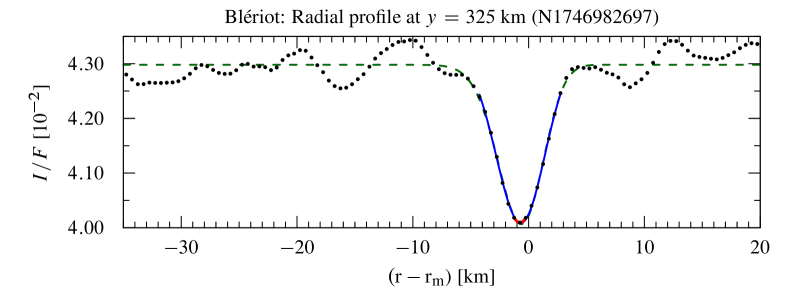
Figure 1: Radial profile of the propeller Blériot 325 km downstream of the moonlet, with clearly visible propeller gap. In order to determine the radial position of the gap-minimum and the gap width, we fit different functions to the radial profile. Shown are fits of Eq. 2 to the complete radial range shown in the plot (dashed dark green curve) and to only the radial range of the propeller gap (blue solid curve). Additionally, the red solid curve is a parabola determined from the data point with the lowest I/F value and its two neighbouring data points.

Fig. 1 shows a radial profile of Blériot 325 km downstream of the moonlet. In order to determine the radial location of the gap minimum in a radial profile, we combine two approaches. First, we determine a parabola from the data point with the lowest I/F value in the gap region and its two neighbouring data points. This local approach is illustrated by the red curve in Fig. 1.

Additionally, we fit the function

$$I/F\left(\xi(x)\right)=\left\{\begin{array}[]{cc}A_{0}-\Delta A\exp\left(-\frac{\left[\ln(\xi)\right]^{2}}{2\eta^{2}\sigma_{\text{gap}}^{2}}\right)&\quad\xi>0\\ A_{0}&\quad\xi\leq 0\end{array}\right.$$ (2)

with $\xi(x)=\eta\left(x-x_{\text{gap}}\right)+1$, to the radial profile data. Here, $A_{0}$ estimates the brightness of the unperturbed ring, $A_{0}-\Delta A$ the brightness at the gap minimum, $x_{\text{gap}}$ the radial location of the gap minimum, and $\sigma_{\text{gap}}$ the width of the gap. The parameter $\eta$ controls the asymmetry around the gap minimum. For $\eta\to 0^{+}$ Eq. 2 turns into a Gaussian profile.

This approach, illustrated by the green dashed and the solid blue curves in Fig. 1, takes the shape of the gap into account. The dashed green curve exemplifies a fit of Eq. 2 to the complete radial range of the radial profile, whereas the solid blue curve shows a fit of Eq. 2 to the radial range of the propeller gap.

The estimates of the location of the gap minimum as calculated from the parabola, the fit of Eq. 2 over the limited radial range, and the fit of Eq. 2 over the complete radial range are $-746\,\text{m}$, $-631\,\text{m}$, and $-678\,\text{m}$, yielding a mean value of $\bar{x}_{\text{gap}}=-685\,\text{m}$ with a root mean square value of about $60\,\text{m}$. For comparison, the projected radial ring plane resolution of the image is $3\,\text{km}/\text{pixel}$, the radial bin-width is $\delta x=500\,\text{m}$ and the azimuthal averaging range is $\delta y=50\,\text{km}$. Depending on the orientation of the propeller in the image, it is often possible to determine radial profiles with sub-pixel resolution.

3 Radial separation of propeller gaps

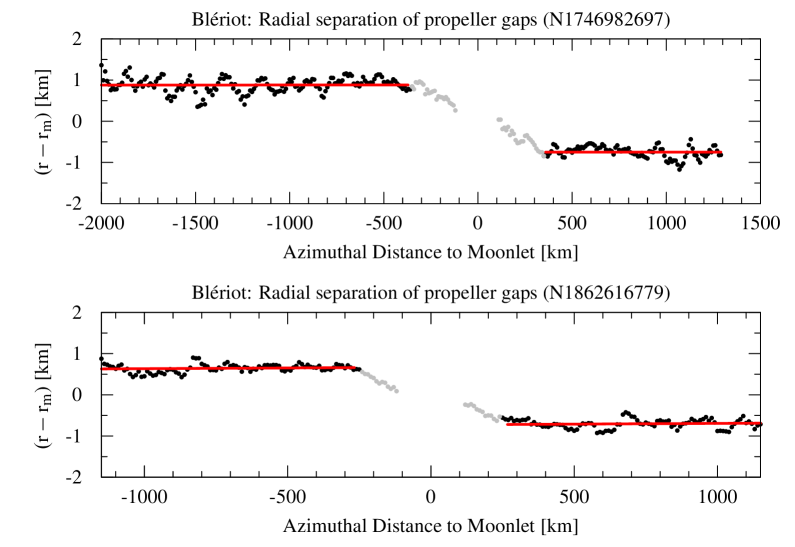
Figure 2: Radial separation of Blériot’s propeller gaps. The plots show the radial distance of gap minima to the moonlet at different azimuthal locations. The red lines are fits of Eq. 3 to the radial gap minima positions quantifying the radial separation of the propeller gaps. Only black data points are used for the fits because the radial gap separation still builds up over the first few hundred kilometers downstream the moonlet.

N-body box simulations (Seiß et al., 2005; Lewis & Stewart, 2009) and hydrodynamical propeller simulations (Seiß et al., 2018) show that the radial separation $\Delta r$ of the gap-minima of the partial propeller gaps is about 4 Hill radii.

We determine the radial separation of the propeller gaps by fitting the function

$$f(y)=\left\{\begin{array}[]{ll}\alpha y+b+\Delta r&\quad y<0\\ \alpha y+b&\quad y>0\end{array}\right.$$ (3)

to radial gap-minima positions at different azimuthal locations. The gap-minima positions are obtained from fits to the different radial profiles prepared for each image as described in Section 2.

Fig. 2 shows two examples of the azimuthal variation of radial gap-minima positions. For the first few hundred kilometers downstream the moonlet the radial separation is still building up (gray data points). Afterwards, the gap-minima positions fluctuate around a mean value (black data points). The red lines illustrate fits of Eq. 3 to the black data points yielding $\Delta r$.

Table 1 lists the fit results for images taken by Cassini’s narrow angle camera (NAC) which show Blériot with clearly visible propeller gaps. These values lead to a Hill radius estimate of $\text{$h$}=(400\pm 100)\,\text{m}$ for Blériot. Seiß et al. (2018) matched results of hydrodynamical propeller simulations to two stellar occultation scans performed by Cassini’s UVIS instrument that scanned through the propeller Blériot. They determined a Hill radius of $\text{$h$}=(600\pm 100)\,\text{m}$ which is larger than our value but lies within a factor of two to each other.

One reason for the difference might be that the relation $\Delta r=4\text{$h$}$ is only approximately valid and that the radial gap-minima separation depends slightly on the azimuthal distance to the moonlet as hydrodynamical simulations suggest. The solution could be to carry out the same analysis performed for the image data for results of these hydrodynamic propeller simulations, but this is still work in progress.

Table 1: Results of radial gap separation fits for Blériot

Image	Radial separation $\Delta r$ [km]	Hill radius $h$ [m]
N1544842586	1.47	370
N1586641169/1255	1.95	510
N1731354160	1.78	445
N1731354280	1.65	410
N1746982697	1.63	410
N1862616735	1.39	350
N1862616779	1.40	350

4 Azimuthal evolution of propeller gaps

4.1 Analytic gap evolution model

Let $\Sigma$ be the ring’s surface mass density. We will assume a power law dependence of the kinematic shear viscosity $\nu$ on the surface mass density

$$\nu(\Sigma)=\nu_{0}\left(\frac{\Sigma}{\Sigma_{0}}\right)^{\!\beta}\ ,$$ (4)

where $\nu_{0}$ and $\Sigma_{0}$ are the shear viscosity and surface mass density of the unperturbed ring. The azimuthal gap relaxation downstream of the propeller moonlet can be described by a linearized viscous diffusion equation (Sremčević et al., 2002)

$$\frac{\partial\!\>\Sigma}{\partial(y/\text{$aK$})}=-(x/\text{$h$})^{-1}\frac{\partial^{\!\>2}\!\>\Sigma}{\partial(x/\text{$h$})^{2}}\$$ (5)

where $aK$ defines the characteristic azimuthal length scale of the viscous diffusion

$$\text{$aK$}=\frac{\Omega_{0}\text{$h$}^{3}}{2(1+\beta)\nu_{0}}\ .$$ (6)

This scaling has been confirmed by N-body (Seiß et al., 2005) and hydrodynamical simulations (Seiß et al., 2018) of propeller structures.

Sremčević et al. (2002) derived an approximate Green’s solution which solves Eq. 5 for $\sigma(x,y=0)=\delta(x-x_{0})$ (where $\sigma=\Sigma-\Sigma_{0}$), which reads

$$G(x,y;x_{0})=-\frac{\sqrt{3}x_{0}}{2\text{$h$}}\left(\frac{3y}{\text{$aK$}}\right)^{-2/3}\exp\left[\frac{(x/\text{$h$})^{3}+(x_{0}/\text{$h$})^{3}}{9(y/\text{$aK$})}\right]\text{Bi}\left[\left(\frac{3y}{\text{$aK$}}\right)^{-2/3}\frac{x_{0}x}{\text{$h$}^{2}}\right]\ .$$ (7)

Here, Bi denotes the Airy function and $\sigma(x,y=0)$ models the scattering of the ring particles by the propeller moonlet.

The general solution is then given by

$$\Sigma(x,y)=\Sigma_{0}+\int\sigma(x_{0},y=0)\,G(x,y;x_{0})\,dx_{0}\ ,$$ (8)

where we will use $\sigma(x,y=0)$ determined from test particle integrations of the Hill problem (Sremčević et al., 2002; Hoffmann et al., 2015).

4.2 Analysis of Cassini NAC images

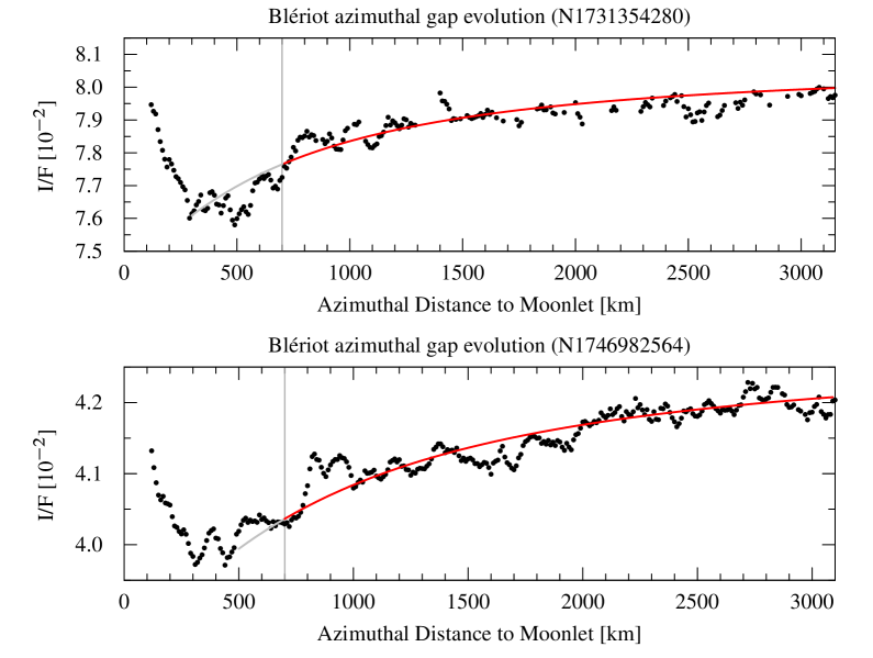
Figure 3: Azimuthal evolution of Blériot’s propeller gaps. The plots show the minimal brightness values in the propeller gap at different azimuthal locations, exemplifying that Blériot’s gaps azimuthally extend for over 3000 km. The red curves illustrate fits of the surface mass density (Eq. 8) to the brightness values, where we used a single-scattering solution to relate the ring’s surface mass density to I/F values. The vertical gray lines mark the starting points of the fits ensuring enough azimuthal distance to the vertically excited region of the propeller, which would not be well described by the isothermal model Eq. 8 is based on.

We determine azimuthal gap profiles by finding the minimal brightness value in the propeller gap for different azimuthal locations from radial profiles. Fig. 3 shows two examples of the azimuthal evolution of Blériot’s propeller gaps extending for over 3000 km. The red curves illustrate fits of the analytical model (Eq. 8) to the azimuthal brightness profiles.

Because we limit our analysis to images of the lit side of the ring, we use a single scattering solution to relate the relative brightness $I/I_{0}$ of the azimuthal profiles to the surface mass density $\Sigma$ of the analytical model

$$\frac{I}{I_{0}}=\frac{1-\exp\left[-\tau\,\frac{\mu+\mu_{0}}{\mu\mu_{0}}\right]}{1-\exp\left[-\tau_{0}\,\frac{\mu+\mu_{0}}{\mu\mu_{0}}\right]}\ ,$$ (9)

where $\mu=|\sin(B)|$ and $\mu_{0}=|\sin(B_{0})|$, $B$ and $B_{0}$ being the elevation angles of the observer and the sun, respectively. Further, we assume that the optical depth $\tau$ is proportional to the surface mass density $\Sigma$, so that $\tau=\tau_{0}\,(\Sigma/\Sigma_{0})$.

In Fig. 3, the fits start $700\,\text{km}$ downstream of the moonlet (depicted by the vertical gray lines) in order to be far away from the vertically excited region of the propeller (Hoffmann et al., 2015, 2013), which would not be well described by the isothermal model Eq. 8 is based on.

The fits result in estimates of the characteristic azimuthal length scale $aK$ which can be used to predict the ring’s kinematic shear viscosity

$$\nu_{0}=\frac{\Omega_{0}\text{$h$}^{3}}{2(1+\beta)\text{$aK$}}\ ,$$ (10)

provided values of the Hill radius $h$ and the power law exponent $\beta$ from Eq. 4 are known. Typical values for $\beta$ determined from N-body box simulations range from $\beta=0.67$ for a ring without self-gravity wakes to $\beta=2$ for fully developed self-gravity wakes (Daisaka et al., 2001; Salo et al., 2018). Further, we use the in Section 3 estimated Hill radius of $400\,\text{m}$ to calculate the kinematic shear viscosity of the ring in the vicinity of Blériot.

Table 2 summarizes estimates for the propeller Blériot. From these values we determine $\text{$aK$}=(235\pm 60)\,\text{km}$ leading to $\nu_{\beta=0.67}=(100\pm 30)\,\text{cm}^{2}/s$ and $\nu_{\beta=2}=(60\pm 20)\,\text{cm}^{2}/s$. These estimates are consistent with the viscosity parametrization used by Daisaka et al. (2001).

Blériot orbits between the Encke and Keeler gaps, a region for which viscosity estimates are still sparse. For the Encke gap edge Tajeddine et al. (2017) estimate $64\,\text{cm}^{2}/s$ and Grätz et al. (2018) find $127\,\text{cm}^{2}/s\leq\nu_{0}\leq 78\,\text{cm}^{2}/s$ for $0\leq\beta\leq 2$. These estimates agree very well with the values we determined. On the other hand, estimates for the Keeler gap edge, $14\,\text{cm}^{2}/s$ (Tajeddine et al., 2017) and $32\,\text{cm}^{2}/s\leq\nu_{0}\leq 20\,\text{cm}^{2}/s$ (Grätz et al., 2018) are smaller than our values.

Table 2: Results of gap evolution fits for Blériot

Image	$aK$ [km]	$\nu_{\beta=0.67}\,[\text{cm}^{2}/\text{s}]$	$\nu_{\beta=2}\,[\text{cm}^{2}/\text{s}]$
N1731354160	216	110	61
N1731354280	224	106	59
N1746982564	275	087	48
N1746982697	276	086	48
N1862616735	198	120	67
N1862616823	222	107	60

Seiß et al. (2018) find a value of $\nu_{0}=(340\pm 120)\,\text{cm}^{2}/s$ by matching isothermal hydrodynamic propeller simulations to UVIS stellar occultation scans. This significantly higher value is very likely overestimated because of the simplified isothermal description of the ring (the UVIS scans intersect the propeller in the vertically excited region of the propeller).

5 Conclusions

The main results of this work are:

1. From the radial separation of Blériot’s propeller gaps in images taken by the Narrow Angle Camera onboard the Cassini spacecraft we estimate the Hill radius of Blériot’s propeller moonlet to be $(400\pm 100)\,\text{m}$.

2. By fitting the analytic solution from Sremčević et al. (2002), which describes the azimuthal evolution of the surface mass density in the propeller gap region, to the azimuthal evolution of the propeller gap obtained from Cassini NAC images, we estimate the kinematic shear viscosity in Blériot’s ring region to be between $\nu_{\beta=2}=(60\pm 20)\,\text{cm}^{2}/s$ and $\nu_{\beta=0.67}=(100\pm 30)\,\text{cm}^{2}/s$.

References

- Baillié et al. (2013) Baillié, K., Colwell, J. E., Esposito, L. W., & Lewis, M. C. 2013, AJ, 145, 171, doi: 10.1088/0004-6256/145/6/171
- Daisaka et al. (2001) Daisaka, H., Tanaka, H., & Ida, S. 2001, Icarus, 154, 296, doi: 10.1006/icar.2001.6716
- Grätz et al. (2018) Grätz, F., Seiß, M., & Spahn, F. 2018, ApJ, 862, 157, doi: 10.3847/1538-4357/aace00
- Hoffmann et al. (2015) Hoffmann, H., Seiß, M., Salo, H., & Spahn, F. 2015, Icarus, 252, 400, doi: 10.1016/j.icarus.2015.02.003
- Hoffmann et al. (2013) Hoffmann, H., Seiß, M., & Spahn, F. 2013, ApJ, 765, L4, doi: 10.1088/2041-8205/765/1/L4
- Lewis & Stewart (2009) Lewis, M. C., & Stewart, G. R. 2009, Icarus, 199, 387, doi: 10.1016/j.icarus.2008.09.009
- Salo et al. (2018) Salo, H., Ohtsuki, K., & Lewis, M. C. 2018, in Planetary Ring Systems, ed. M. S. Tiscareno & C. D. Murray (Cambridge University Press), 462
- Seiß et al. (2018) Seiß, M., Albers, N., Sremčević, M., et al. 2018, Accepted for publication in Astronomical Journal, (arXiv:1701.04641v2)
- Seiß et al. (2005) Seiß, M., Spahn, F., Sremčević, M., & Salo, H. 2005, Geophys. Res. Lett., 32, 11205, doi: 10.1029/2005GL022506
- Spahn & Sremčević (2000) Spahn, F., & Sremčević, M. 2000, A&A, 358, 368
- Sremčević et al. (2007) Sremčević, M., Schmidt, J., Salo, H., et al. 2007, Nature, 449, 1019, doi: 10.1038/nature06224
- Sremčević et al. (2002) Sremčević, M., Spahn, F., & Duschl, W. J. 2002, MNRAS, 337, 1139, doi: 10.1046/j.1365-8711.2002.06011.x
- Tajeddine et al. (2017) Tajeddine, R., Nicholson, P. D., Longaretti, P.-Y., El Moutamid, M., & Burns, J. A. 2017, ApJS, 232, 28, doi: 10.3847/1538-4365/aa8c09
- Tiscareno et al. (2008) Tiscareno, M. S., Burns, J. A., Hedman, M. M., & Porco, C. C. 2008, AJ, 135, 1083, doi: 10.1088/0004-6256/135/3/1083
- Tiscareno et al. (2006) Tiscareno, M. S., Burns, J. A., Hedman, M. M., et al. 2006, Nature, 440, 648, doi: 10.1038/nature04581
- Tiscareno et al. (2010) Tiscareno, M. S., Burns, J. A., Sremčević, M., et al. 2010, ApJ, 718, L92, doi: 10.1088/2041-8205/718/2/L92