Adaptive model selection method for a conditionally Gaussian semimartingale regression in continuous time

Abstract

This paper considers the problem of robust adaptive efficient estimating of a periodic function in a continuous time regression model with the dependent noises given by a general square integrable semimartingale with a conditionally Gaussian distribution. An example of such noise is the non-Gaussian Ornstein–Uhlenbeck–Lévy processes. An adaptive model selection procedure, based on the improved weighted least square estimates, is proposed. Under some conditions on the noise distribution, sharp oracle inequality for the robust risk has been proved and the robust efficiency of the model selection procedure has been established. The numerical analysis results are given.

Key words: Improved non-asymptotic estimation, Least squares estimates, Robust quadratic risk, Non-parametric regression, Semimartingale noise, Ornstein–Uhlenbeck–Lévy process, Model selection, Sharp oracle inequality, Asymptotic efficiency.

UDC : 519.2

1 Introduction

Consider a regression model in continuous time

$$\mathrm{d}y_{t}=S(t)\mathrm{d}t+\mathrm{d}\xi_{t}\,,\quad 0\leq t\leq n\,,$$ (1.1)

where $S$ is an unknown $1$-periodic ${\mathbb{R}}\to{\mathbb{R}}$ function, $S\in{\bf L}_{\mathchoice{2}{2}{\lower 0.75346pt\hbox{$\scriptstyle 2$}}{\lower 0.75346pt\hbox{$\scriptscriptstyle 2$}}}[0,1]$; $(\xi_{\mathchoice{t}{t}{\lower 0.75346pt\hbox{$\scriptstyle t$}}{\lower 0.75346pt\hbox{$\scriptscriptstyle t$}}})_{\mathchoice{t\geq 0}{t\geq 0}{\lower 0.75346pt\hbox{$\scriptstyle t\geq 0$}}{\lower 0.75346pt\hbox{$\scriptscriptstyle t\geq 0$}}}$ is an unobservable conditionally Gaussian semimartingale with the values in the Skorokhod space ${\bf D}[0,n]$ such that, for any cadlag $[0,n]\to{\mathbb{R}}$ function $f$ from ${\bf L}_{\mathchoice{2}{2}{\lower 0.75346pt\hbox{$\scriptstyle 2$}}{\lower 0.75346pt\hbox{$\scriptscriptstyle 2$}}}[0,n]$, the stochastic integral

$$I_{\mathchoice{n}{n}{\lower 0.75346pt\hbox{$\scriptstyle n$}}{\lower 0.75346pt\hbox{$\scriptscriptstyle n$}}}(f)=\int^{n}_{\mathchoice{0}{0}{\lower 0.75346pt\hbox{$\scriptstyle 0$}}{\lower 0.75346pt\hbox{$\scriptscriptstyle 0$}}}f(s)\mathrm{d}\xi_{\mathchoice{s}{s}{\lower 0.75346pt\hbox{$\scriptstyle s$}}{\lower 0.75346pt\hbox{$\scriptscriptstyle s$}}}$$ (1.2)

is well defined and has the following properties

$${\bf E}_{\mathchoice{Q}{Q}{\lower 0.75346pt\hbox{$\scriptstyle Q$}}{\lower 0.75346pt\hbox{$\scriptscriptstyle Q$}}}I_{\mathchoice{n}{n}{\lower 0.75346pt\hbox{$\scriptstyle n$}}{\lower 0.75346pt\hbox{$\scriptscriptstyle n$}}}(f)=0\quad\mbox{and}\quad{\bf E}_{\mathchoice{Q}{Q}{\lower 0.75346pt\hbox{$\scriptstyle Q$}}{\lower 0.75346pt\hbox{$\scriptscriptstyle Q$}}}I^{2}_{\mathchoice{n}{n}{\lower 0.75346pt\hbox{$\scriptstyle n$}}{\lower 0.75346pt\hbox{$\scriptscriptstyle n$}}}(f)\leq\varkappa_{\mathchoice{Q}{Q}{\lower 0.75346pt\hbox{$\scriptstyle Q$}}{\lower 0.75346pt\hbox{$\scriptscriptstyle Q$}}}\int^{n}_{\mathchoice{0}{0}{\lower 0.75346pt\hbox{$\scriptstyle 0$}}{\lower 0.75346pt\hbox{$\scriptscriptstyle 0$}}}\,f^{2}(s)\mathrm{d}s\,.$$ (1.3)

Here ${\bf E}_{\mathchoice{Q}{Q}{\lower 0.75346pt\hbox{$\scriptstyle Q$}}{\lower 0.75346pt\hbox{$\scriptscriptstyle Q$}}}$ denotes the expectation with respect to the distribution $Q$ of the noise process $(\xi_{\mathchoice{t}{t}{\lower 0.75346pt\hbox{$\scriptstyle t$}}{\lower 0.75346pt\hbox{$\scriptscriptstyle t$}}})_{\mathchoice{0\leq t\leq n}{0\leq t\leq n}{\lower 0.75346pt\hbox{$\scriptstyle 0\leq t\leq n$}}{\lower 0.75346pt\hbox{$\scriptscriptstyle 0\leq t\leq n$}}}$ on the space ${\cal D}[0,n]$; $\varkappa_{\mathchoice{Q}{Q}{\lower 0.75346pt\hbox{$\scriptstyle Q$}}{\lower 0.75346pt\hbox{$\scriptscriptstyle Q$}}}>0$ is some positive constant depending on the distribution $Q$. The noise distribution $Q$ is unknown and assumed to belong to some probability family ${\cal Q}_{\mathchoice{n}{n}{\lower 0.75346pt\hbox{$\scriptstyle n$}}{\lower 0.75346pt\hbox{$\scriptscriptstyle n$}}}$ specified below. All necessary tools concerning the stochastic calculus can be found, for example, in [13].

The class of the disturbances $\xi$ satisfying conditions (1.3) is rather wide and comprises, in particular, the Lévy processes which are used in different applied problems (see [4], for details). The models (1.1) with the Lévy’s type noise naturally arise in the nonparametric functional statistics problems (see, for example, [8, 15, 16]). Moreover, as is shown in Section 2, non-Gaussian Ornstein–Uhlenbeck-based models, introduced in [2], enter this class. It is well-known that in the filtration theory the assumption of the conditional gaussinity of the unobserved process with respect to the observed one led to the extension of the classical Kalman–Bucy problem with the closed form solution to a class of the stochastic models described by the equations including nonlinearly the process under observation [21].

The problem is to estimate the unknown function $S$ in the model (1.1) on the basis of observations $(y_{\mathchoice{t}{t}{\lower 0.75346pt\hbox{$\scriptstyle t$}}{\lower 0.75346pt\hbox{$\scriptscriptstyle t$}}})_{\mathchoice{0\leq t\leq n}{0\leq t\leq n}{\lower 0.75346pt\hbox{$\scriptstyle 0\leq t\leq n$}}{\lower 0.75346pt\hbox{$\scriptscriptstyle 0\leq t\leq n$}}}$.

We define the error of an estimate $\widehat{S}$ (any real-valued function measurable with respect to $\sigma\{y_{\mathchoice{t}{t}{\lower 0.75346pt\hbox{$\scriptstyle t$}}{\lower 0.75346pt\hbox{$\scriptscriptstyle t$}}}\,,\,0\leq t\leq n\}$) for $S$ by its integral quadratic risk

$${\cal R}_{\mathchoice{Q}{Q}{\lower 0.75346pt\hbox{$\scriptstyle Q$}}{\lower 0.75346pt\hbox{$\scriptscriptstyle Q$}}}(\widehat{S},S):={\bf E}_{\mathchoice{Q,S}{Q,S}{\lower 0.75346pt\hbox{$\scriptstyle Q,S$}}{\lower 0.75346pt\hbox{$\scriptscriptstyle Q,S$}}}\,\|\widehat{S}-S\|^{2}\,,$$ (1.4)

where ${\bf E}_{\mathchoice{Q,S}{Q,S}{\lower 0.75346pt\hbox{$\scriptstyle Q,S$}}{\lower 0.75346pt\hbox{$\scriptscriptstyle Q,S$}}}$ stands for the expectation with respect to the distribution ${\bf P}_{\mathchoice{Q,S}{Q,S}{\lower 0.75346pt\hbox{$\scriptstyle Q,S$}}{\lower 0.75346pt\hbox{$\scriptscriptstyle Q,S$}}}$ of the process (1.1) with a fixed distribution $Q$ of the noise $(\xi_{\mathchoice{t}{t}{\lower 0.75346pt\hbox{$\scriptstyle t$}}{\lower 0.75346pt\hbox{$\scriptscriptstyle t$}}})_{\mathchoice{0\leq t\leq n}{0\leq t\leq n}{\lower 0.75346pt\hbox{$\scriptstyle 0\leq t\leq n$}}{\lower 0.75346pt\hbox{$\scriptscriptstyle 0\leq t\leq n$}}}$ and a given function $S$; $\|\cdot\|$ is the norm in ${\cal L}_{\mathchoice{2}{2}{\lower 0.75346pt\hbox{$\scriptstyle 2$}}{\lower 0.75346pt\hbox{$\scriptscriptstyle 2$}}}[0,1]$, i.e.

$$\|f\|^{2}:=\int^{1}_{\mathchoice{0}{0}{\lower 0.75346pt\hbox{$\scriptstyle 0$}}{\lower 0.75346pt\hbox{$\scriptscriptstyle 0$}}}f^{2}(t)\mathrm{d}t\,.$$

Since in our case the noise distribution $Q$ is unknown, we will measure the quality of an estimate $\widehat{S}$ by the robust risk defined as

$${\cal R}^{*}_{\mathchoice{n}{n}{\lower 0.75346pt\hbox{$\scriptstyle n$}}{\lower 0.75346pt\hbox{$\scriptscriptstyle n$}}}(\widehat{S},S)=\sup_{\mathchoice{Q\in{\cal Q}_{\mathchoice{n}{n}{\lower 0.5382pt\hbox{$\scriptstyle n$}}{\lower 0.5382pt\hbox{$\scriptscriptstyle n$}}}}{Q\in{\cal Q}_{\mathchoice{n}{n}{\lower 0.5382pt\hbox{$\scriptstyle n$}}{\lower 0.5382pt\hbox{$\scriptscriptstyle n$}}}}{\lower 0.75346pt\hbox{$\scriptstyle Q\in{\cal Q}_{\mathchoice{n}{n}{\lower 0.37672pt\hbox{$\scriptstyle n$}}{\lower 0.37672pt\hbox{$\scriptscriptstyle n$}}}$}}{\lower 0.75346pt\hbox{$\scriptscriptstyle Q\in{\cal Q}_{\mathchoice{n}{n}{\lower 0.37672pt\hbox{$\scriptstyle n$}}{\lower 0.37672pt\hbox{$\scriptscriptstyle n$}}}$}}}\,{\cal R}_{\mathchoice{Q}{Q}{\lower 0.75346pt\hbox{$\scriptstyle Q$}}{\lower 0.75346pt\hbox{$\scriptscriptstyle Q$}}}(\widehat{S},S)$$ (1.5)

which assumes taking supremum of the error (1.4) over the whole family of admissible distributions ${\cal Q}_{\mathchoice{n}{n}{\lower 0.75346pt\hbox{$\scriptstyle n$}}{\lower 0.75346pt\hbox{$\scriptscriptstyle n$}}}$ (see, for example, [9]).

We will study the stated problem from the standpoint of the model selection approach. approach. It will be noted that the origin of this method goes back to papers by Akaike [1] and Mallows [22]. The further progress has been made by Barron, Birgé and Massart [3, 24], who developed a non-asymptotic model selection method which enables one to derive nonasymptotic oracle inequalities for nonparametric regression models with the i.i.d. Gaussian disturbances. Fourdrinier and Pergamenshchikov [7] extended the Barron Birgé Massart method to the models with the spherically symmetric dependent observations. The authors in [17] applied this method to the nonparametric problem of estimating a periodic function in a continuous time model with a Gaussian colored noise. Unfortunately, the oracle inequalities obtained in these papers can not provide the efficient estimation in the adaptive setting. For constructing adaptive procedures in our case one needs to use the approach based on the sharp oracle inequalities, proposed by Galtchouk and Pergamenshchikov [10, 11] for the heteroscedastic regression models in discrete time and which developed by Konev and Pergamenshchikov [18, 19] for nonparametric regression models in continuous time.

The goal of this paper is to develop the adaptive robust efficient model selection method for the regression (1.1) with dependent noises having conditionally Gaussian distribution using the improved estimation approach. This paper proposes the shrinkage least squares estimates which enable us to improve the non-asymptotic estimation accuracy. For the first time such idea was proposed by Fourdrinier and Pergamenshchikov in [7] for regression models in discrete time and by Konev and Pergamenshchikov in [17] for Gaussian regression models in continuous time. We develop these methods for the general semimartingale regression models in continuous time. It should be noted that for the conditionally Gaussian regression models we can not use the well-known improved estimators proposed in [14] for Gaussian or spherically symmetric observations. To apply the improved estimation methods to the non-Gaussian regression models in continuous time one needs to use the modifications of the well-known James - Stein estimators proposed in [20, 28] for parametric problems. We develop the new analytical tools which allow one to obtain the sharp non-asymptotic oracle inequalities for robust risks under general conditions on the distribution of the noise in the model (1.1). This method enables us to treat both the cases of dependent and independent observations from the same standpoint, it does not assume the knowledge of the noise distribution and leads to the efficient estimation procedure with respect to the risk (1.5). The validity of the conditions, imposed on the noise in the equation (1.1) is verified for a non-Gaussian Ornstein–Uhlenbeck process.

The rest of the paper is organized as follows. In the next Section 2, we describe the Ornstein–Uhlenbeck process as the example of a semimartingale noise in the model (1.1). In Section 3 we construct the shrinkage weighted least squares estimates and study the improvement effect. In Section 4 we construct the model selection procedure on the basis of improved weighted least squares estimates and state the main results in the form of oracle inequalities for the quadratic risk (1.4) and the robust risk (1.5). In Section 5 it is shown that the proposed model selection procedure for estimating $S$ in (1.1) is asymptotically efficient with respect to the robust risk (1.5). In Section 6 we illustrate the performance of the proposed model selection procedure through numerical simulations. In Section 7 we establish some properties of the stochastic integrals with respect to the non-Gaussian Ornstein- Uhlenbeck process (2.1). Section 8 gives the proofs of the main results. In the Appendix some auxiliary lemmas are given.

2 Ornstein-Uhlenbeck-Lévy process

Now we consider the noise process $(\xi_{\mathchoice{t}{t}{\lower 0.75346pt\hbox{$\scriptstyle t$}}{\lower 0.75346pt\hbox{$\scriptscriptstyle t$}}})_{\mathchoice{t\geq 0}{t\geq 0}{\lower 0.75346pt\hbox{$\scriptstyle t\geq 0$}}{\lower 0.75346pt\hbox{$\scriptscriptstyle t\geq 0$}}}$ in (1.1) defined by a non-Gaussian Ornstein–Uhlenbeck process with the Lévy subordinator. Such processes are used in the financial Black–Scholes type markets with jumps (see, for example, [6] and the references therein). Let the noise process in (1.1) obeys the equation

$$\mathrm{d}\xi_{\mathchoice{t}{t}{\lower 0.75346pt\hbox{$\scriptstyle t$}}{\lower 0.75346pt\hbox{$\scriptscriptstyle t$}}}=a\xi_{\mathchoice{t}{t}{\lower 0.75346pt\hbox{$\scriptstyle t$}}{\lower 0.75346pt\hbox{$\scriptscriptstyle t$}}}\mathrm{d}t+\mathrm{d}u_{\mathchoice{t}{t}{\lower 0.75346pt\hbox{$\scriptstyle t$}}{\lower 0.75346pt\hbox{$\scriptscriptstyle t$}}}\,,\quad\xi_{\mathchoice{0}{0}{\lower 0.75346pt\hbox{$\scriptstyle 0$}}{\lower 0.75346pt\hbox{$\scriptscriptstyle 0$}}}=0\,,$$ (2.1)

where

$$u_{\mathchoice{t}{t}{\lower 0.75346pt\hbox{$\scriptstyle t$}}{\lower 0.75346pt\hbox{$\scriptscriptstyle t$}}}=\varrho_{\mathchoice{1}{1}{\lower 0.75346pt\hbox{$\scriptstyle 1$}}{\lower 0.75346pt\hbox{$\scriptscriptstyle 1$}}}\,w_{\mathchoice{t}{t}{\lower 0.75346pt\hbox{$\scriptstyle t$}}{\lower 0.75346pt\hbox{$\scriptscriptstyle t$}}}+\varrho_{\mathchoice{2}{2}{\lower 0.75346pt\hbox{$\scriptstyle 2$}}{\lower 0.75346pt\hbox{$\scriptscriptstyle 2$}}}\,z_{\mathchoice{t}{t}{\lower 0.75346pt\hbox{$\scriptstyle t$}}{\lower 0.75346pt\hbox{$\scriptscriptstyle t$}}}\quad\mbox{and}\quad z_{\mathchoice{t}{t}{\lower 0.75346pt\hbox{$\scriptstyle t$}}{\lower 0.75346pt\hbox{$\scriptscriptstyle t$}}}=\int_{\mathchoice{{\mathbb{R}}}{{\mathbb{R}}}{\lower 0.75346pt\hbox{$\scriptstyle{\mathbb{R}}$}}{\lower 0.75346pt\hbox{$\scriptscriptstyle{\mathbb{R}}$}}}\,x*(\mu-\widetilde{\mu})_{\mathchoice{t}{t}{\lower 0.75346pt\hbox{$\scriptstyle t$}}{\lower 0.75346pt\hbox{$\scriptscriptstyle t$}}}\,.$$ (2.2)

Here $(w_{\mathchoice{t}{t}{\lower 0.75346pt\hbox{$\scriptstyle t$}}{\lower 0.75346pt\hbox{$\scriptscriptstyle t$}}})_{\mathchoice{t\geq 0}{t\geq 0}{\lower 0.75346pt\hbox{$\scriptstyle t\geq 0$}}{\lower 0.75346pt\hbox{$\scriptscriptstyle t\geq 0$}}}$ is a standard Brownian motion, $\mu(\mathrm{d}s\,\mathrm{d}x)$ is the jump measure with the deterministic compensator $\widetilde{\mu}(\mathrm{d}s\,\mathrm{d}x)=\mathrm{d}s\Pi(\mathrm{d}x)$, $\Pi(\cdot)$ is a Lévy measure, i.e. some positive measure on ${\mathbb{R}}_{\mathchoice{*}{*}{\lower 0.75346pt\hbox{$\scriptstyle*$}}{\lower 0.75346pt\hbox{$\scriptscriptstyle*$}}}={\mathbb{R}}\setminus\{0\}$, see, for example [5, 13], such that

$$\Pi(x^{2})=1\quad\mbox{and}\quad\Pi(x^{8})\,<\,\infty\,.$$ (2.3)

We use the notation $\Pi(|x|^{m})=\int_{\mathchoice{{\mathbb{R}}_{\mathchoice{*}{*}{\lower 0.5382pt\hbox{$\scriptstyle*$}}{\lower 0.5382pt\hbox{$\scriptscriptstyle*$}}}}{{\mathbb{R}}_{\mathchoice{*}{*}{\lower 0.5382pt\hbox{$\scriptstyle*$}}{\lower 0.5382pt\hbox{$\scriptscriptstyle*$}}}}{\lower 0.75346pt\hbox{$\scriptstyle{\mathbb{R}}_{\mathchoice{*}{*}{\lower 0.37672pt\hbox{$\scriptstyle*$}}{\lower 0.37672pt\hbox{$\scriptscriptstyle*$}}}$}}{\lower 0.75346pt\hbox{$\scriptscriptstyle{\mathbb{R}}_{\mathchoice{*}{*}{\lower 0.37672pt\hbox{$\scriptstyle*$}}{\lower 0.37672pt\hbox{$\scriptscriptstyle*$}}}$}}}\,|z|^{m}\,\Pi(\mathrm{d}z)$. Note that the Lévy measure $\Pi({\mathbb{R}}_{\mathchoice{*}{*}{\lower 0.75346pt\hbox{$\scriptstyle*$}}{\lower 0.75346pt\hbox{$\scriptscriptstyle*$}}})$ could be equal to $+\infty$.

We assume that the nuisance parameters $a\leq 0$, $\varrho_{\mathchoice{1}{1}{\lower 0.75346pt\hbox{$\scriptstyle 1$}}{\lower 0.75346pt\hbox{$\scriptscriptstyle 1$}}}$ and $\varrho_{\mathchoice{2}{2}{\lower 0.75346pt\hbox{$\scriptstyle 2$}}{\lower 0.75346pt\hbox{$\scriptscriptstyle 2$}}}$ satisfy the conditions

$$-a_{\mathchoice{max}{max}{\lower 0.75346pt\hbox{$\scriptstyle max$}}{\lower 0.75346pt\hbox{$\scriptscriptstyle max$}}}\leq a\leq 0\,,\quad 0<\underline{\varrho}\leq\varrho^{2}_{\mathchoice{1}{1}{\lower 0.75346pt\hbox{$\scriptstyle 1$}}{\lower 0.75346pt\hbox{$\scriptscriptstyle 1$}}}\quad\mbox{and}\quad\sigma_{\mathchoice{Q}{Q}{\lower 0.75346pt\hbox{$\scriptstyle Q$}}{\lower 0.75346pt\hbox{$\scriptscriptstyle Q$}}}=\varrho^{2}_{\mathchoice{1}{1}{\lower 0.75346pt\hbox{$\scriptstyle 1$}}{\lower 0.75346pt\hbox{$\scriptscriptstyle 1$}}}+\varrho^{2}_{\mathchoice{2}{2}{\lower 0.75346pt\hbox{$\scriptstyle 2$}}{\lower 0.75346pt\hbox{$\scriptscriptstyle 2$}}}\,\leq\varsigma^{*}\,,$$ (2.4)

where the bounds $a_{\mathchoice{max}{max}{\lower 0.75346pt\hbox{$\scriptstyle max$}}{\lower 0.75346pt\hbox{$\scriptscriptstyle max$}}}$, $\underline{\varrho}$ and $\varsigma^{*}$ are functions of $n$, i.e. $a_{\mathchoice{max}{max}{\lower 0.75346pt\hbox{$\scriptstyle max$}}{\lower 0.75346pt\hbox{$\scriptscriptstyle max$}}}=a_{\mathchoice{max}{max}{\lower 0.75346pt\hbox{$\scriptstyle max$}}{\lower 0.75346pt\hbox{$\scriptscriptstyle max$}}}(n)$, $\underline{\varrho}=\varrho_{\mathchoice{n}{n}{\lower 0.75346pt\hbox{$\scriptstyle n$}}{\lower 0.75346pt\hbox{$\scriptscriptstyle n$}}}$ and $\varsigma^{*}=\varsigma^{*}_{\mathchoice{n}{n}{\lower 0.75346pt\hbox{$\scriptstyle n$}}{\lower 0.75346pt\hbox{$\scriptscriptstyle n$}}}$, such that for any $\check{\delta}>0$

$$\lim_{\mathchoice{n\to\infty}{n\to\infty}{\lower 0.75346pt\hbox{$\scriptstyle n\to\infty$}}{\lower 0.75346pt\hbox{$\scriptscriptstyle n\to\infty$}}}\,\frac{a_{\mathchoice{max}{max}{\lower 0.75346pt\hbox{$\scriptstyle max$}}{\lower 0.75346pt\hbox{$\scriptscriptstyle max$}}}(n)}{n^{\epsilon}}=0\,,\quad\liminf_{\mathchoice{n\to\infty}{n\to\infty}{\lower 0.75346pt\hbox{$\scriptstyle n\to\infty$}}{\lower 0.75346pt\hbox{$\scriptscriptstyle n\to\infty$}}}\,n^{\epsilon}\,\underline{\varrho}_{\mathchoice{n}{n}{\lower 0.75346pt\hbox{$\scriptstyle n$}}{\lower 0.75346pt\hbox{$\scriptscriptstyle n$}}}\,>0\quad\mbox{and}\quad\lim_{\mathchoice{n\to\infty}{n\to\infty}{\lower 0.75346pt\hbox{$\scriptstyle n\to\infty$}}{\lower 0.75346pt\hbox{$\scriptscriptstyle n\to\infty$}}}\,n^{-\epsilon}\,\varsigma^{*}_{\mathchoice{n}{n}{\lower 0.75346pt\hbox{$\scriptstyle n$}}{\lower 0.75346pt\hbox{$\scriptscriptstyle n$}}}=0\,.$$ (2.5)

We denote by ${\cal Q}_{\mathchoice{n}{n}{\lower 0.75346pt\hbox{$\scriptstyle n$}}{\lower 0.75346pt\hbox{$\scriptscriptstyle n$}}}$ the family of all distributions of process (1.1) – (2.1) on the Skorokhod space ${\bf D}[0,n]$ satisfying the conditions (2.4) – (2.5).

It should be noted that in view of Corollary 7.2 the condition (1.3) for the process (2.1) holds with

$$\varkappa_{\mathchoice{Q}{Q}{\lower 0.75346pt\hbox{$\scriptstyle Q$}}{\lower 0.75346pt\hbox{$\scriptscriptstyle Q$}}}=2\varrho_{\mathchoice{*}{*}{\lower 0.75346pt\hbox{$\scriptstyle*$}}{\lower 0.75346pt\hbox{$\scriptscriptstyle*$}}}\,.$$ (2.6)

Note also that the process (2.1) is conditionally-Gaussian square integrated semimartingale with respect to $\sigma$-algebra ${\cal G}=\sigma\{z_{\mathchoice{t}{t}{\lower 0.75346pt\hbox{$\scriptstyle t$}}{\lower 0.75346pt\hbox{$\scriptscriptstyle t$}}}\,,\,t\geq 0\}$ which is generated by jump process $(z_{t})_{t\geq 0}$.

3 Shrinkage estimates

For estimating the unknown function $S$ in (1.1) we will consider it’s Fourier expansion. Let $(\phi_{\mathchoice{j}{j}{\lower 0.75346pt\hbox{$\scriptstyle j$}}{\lower 0.75346pt\hbox{$\scriptscriptstyle j$}}})_{\mathchoice{j\geq\,1}{j\geq\,1}{\lower 0.75346pt\hbox{$\scriptstyle j\geq\,1$}}{\lower 0.75346pt\hbox{$\scriptscriptstyle j\geq\,1$}}}$ be an orthonormal basis in ${\bf L}_{\mathchoice{2}{2}{\lower 0.75346pt\hbox{$\scriptstyle 2$}}{\lower 0.75346pt\hbox{$\scriptscriptstyle 2$}}}[0,1]$. We extend these functions by the periodic way on ${\mathbb{R}}$, i.e. $\phi_{\mathchoice{j}{j}{\lower 0.75346pt\hbox{$\scriptstyle j$}}{\lower 0.75346pt\hbox{$\scriptscriptstyle j$}}}(t)$=$\phi_{\mathchoice{j}{j}{\lower 0.75346pt\hbox{$\scriptstyle j$}}{\lower 0.75346pt\hbox{$\scriptscriptstyle j$}}}(t+1)$ for any $t\in{\mathbb{R}}$.

${\bf B}_{\mathchoice{1}{1}{\lower 0.75346pt\hbox{$\scriptstyle 1$}}{\lower 0.75346pt\hbox{$\scriptscriptstyle 1$}}}$) Assume that the basis functions are uniformly bounded, i.e. for some constant $\phi_{\mathchoice{*}{*}{\lower 0.75346pt\hbox{$\scriptstyle*$}}{\lower 0.75346pt\hbox{$\scriptscriptstyle*$}}}\geq 1$, which may be depend on $n$,

$$\sup_{\mathchoice{0\leq j\leq n}{0\leq j\leq n}{\lower 0.75346pt\hbox{$\scriptstyle 0\leq j\leq n$}}{\lower 0.75346pt\hbox{$\scriptscriptstyle 0\leq j\leq n$}}}\,\sup_{\mathchoice{0\leq t\leq 1}{0\leq t\leq 1}{\lower 0.75346pt\hbox{$\scriptstyle 0\leq t\leq 1$}}{\lower 0.75346pt\hbox{$\scriptscriptstyle 0\leq t\leq 1$}}}|\phi_{\mathchoice{j}{j}{\lower 0.75346pt\hbox{$\scriptstyle j$}}{\lower 0.75346pt\hbox{$\scriptscriptstyle j$}}}(t)|\,\leq\,\phi_{\mathchoice{*}{*}{\lower 0.75346pt\hbox{$\scriptstyle*$}}{\lower 0.75346pt\hbox{$\scriptscriptstyle*$}}}<\infty\,.$$ (3.1)

${\bf B}_{\mathchoice{2}{2}{\lower 0.75346pt\hbox{$\scriptstyle 2$}}{\lower 0.75346pt\hbox{$\scriptscriptstyle 2$}}}$) Assume that there exist some $d_{\mathchoice{0}{0}{\lower 0.75346pt\hbox{$\scriptstyle 0$}}{\lower 0.75346pt\hbox{$\scriptscriptstyle 0$}}}\geq 7$ and $\check{a}\geq 1$ such that

$$\sup_{\mathchoice{d\geq d_{\mathchoice{0}{0}{\lower 0.5382pt\hbox{$\scriptstyle 0$}}{\lower 0.5382pt\hbox{$\scriptscriptstyle 0$}}}}{d\geq d_{\mathchoice{0}{0}{\lower 0.5382pt\hbox{$\scriptstyle 0$}}{\lower 0.5382pt\hbox{$\scriptscriptstyle 0$}}}}{\lower 0.75346pt\hbox{$\scriptstyle d\geq d_{\mathchoice{0}{0}{\lower 0.37672pt\hbox{$\scriptstyle 0$}}{\lower 0.37672pt\hbox{$\scriptscriptstyle 0$}}}$}}{\lower 0.75346pt\hbox{$\scriptscriptstyle d\geq d_{\mathchoice{0}{0}{\lower 0.37672pt\hbox{$\scriptstyle 0$}}{\lower 0.37672pt\hbox{$\scriptscriptstyle 0$}}}$}}}\,\frac{1}{d}\,\int^{1}_{\mathchoice{0}{0}{\lower 0.75346pt\hbox{$\scriptstyle 0$}}{\lower 0.75346pt\hbox{$\scriptscriptstyle 0$}}}\,\Phi^{*}_{\mathchoice{d}{d}{\lower 0.75346pt\hbox{$\scriptstyle d$}}{\lower 0.75346pt\hbox{$\scriptscriptstyle d$}}}(v)\,\mathrm{d}v\leq\,\check{a}\,,$$ (3.2)

where $\Phi^{*}_{\mathchoice{d}{d}{\lower 0.75346pt\hbox{$\scriptstyle d$}}{\lower 0.75346pt\hbox{$\scriptscriptstyle d$}}}(v)=\max_{\mathchoice{t\geq v}{t\geq v}{\lower 0.75346pt\hbox{$\scriptstyle t\geq v$}}{\lower 0.75346pt\hbox{$\scriptscriptstyle t\geq v$}}}\left|\sum^{d}_{\mathchoice{j=1}{j=1}{\lower 0.75346pt\hbox{$\scriptstyle j=1$}}{\lower 0.75346pt\hbox{$\scriptscriptstyle j=1$}}}\,\phi_{\mathchoice{j}{j}{\lower 0.75346pt\hbox{$\scriptstyle j$}}{\lower 0.75346pt\hbox{$\scriptscriptstyle j$}}}(t)\,\phi_{\mathchoice{j}{j}{\lower 0.75346pt\hbox{$\scriptstyle j$}}{\lower 0.75346pt\hbox{$\scriptscriptstyle j$}}}(t-v)\right|$.

For example, we can take the trigonometric basis defined as $\mbox{Tr}_{\mathchoice{1}{1}{\lower 0.75346pt\hbox{$\scriptstyle 1$}}{\lower 0.75346pt\hbox{$\scriptscriptstyle 1$}}}\equiv 1$ and for $j\geq 2$

$$\mbox{Tr}_{\mathchoice{j}{j}{\lower 0.75346pt\hbox{$\scriptstyle j$}}{\lower 0.75346pt\hbox{$\scriptscriptstyle j$}}}(x)=\sqrt{2}\left\{\begin{array}[]{c}\cos(\varpi_{\mathchoice{j}{j}{\lower 0.75346pt\hbox{$\scriptstyle j$}}{\lower 0.75346pt\hbox{$\scriptscriptstyle j$}}}x)\,\quad\mbox{for even}\quad j\,;\\[11.38109pt] \sin(\varpi_{\mathchoice{j}{j}{\lower 0.75346pt\hbox{$\scriptstyle j$}}{\lower 0.75346pt\hbox{$\scriptscriptstyle j$}}}x)\quad\mbox{for odd}\quad j\,,\end{array}\right.$$ (3.3)

where the frequency $\varpi_{\mathchoice{j}{j}{\lower 0.75346pt\hbox{$\scriptstyle j$}}{\lower 0.75346pt\hbox{$\scriptscriptstyle j$}}}=2\pi[j/2]$ and $[x]$ denotes integer part of $x$.

In Lemma A.1 we shown that these functions satisfy the condition ${\bf B}_{\mathchoice{2}{2}{\lower 0.75346pt\hbox{$\scriptstyle 2$}}{\lower 0.75346pt\hbox{$\scriptscriptstyle 2$}}}$) with

$$d_{\mathchoice{0}{0}{\lower 0.75346pt\hbox{$\scriptstyle 0$}}{\lower 0.75346pt\hbox{$\scriptscriptstyle 0$}}}=\inf\{d\geq 7\,:\,5+\ln d\leq\check{a}d\}\quad\mbox{and}\quad\check{a}=(1-e^{-a_{\mathchoice{max}{max}{\lower 0.5382pt\hbox{$\scriptstyle max$}}{\lower 0.5382pt\hbox{$\scriptscriptstyle max$}}}})/(4a_{\mathchoice{max}{max}{\lower 0.75346pt\hbox{$\scriptstyle max$}}{\lower 0.75346pt\hbox{$\scriptscriptstyle max$}}})\,.$$ (3.4)

We write the Fourier expansion of the unknown function $S$ in the form

$$S(t)=\sum_{j=1}^{\infty}\theta_{\mathchoice{j}{j}{\lower 0.75346pt\hbox{$\scriptstyle j$}}{\lower 0.75346pt\hbox{$\scriptscriptstyle j$}}}\phi_{j}(t),$$

where the corresponding Fourier coefficients

$$\theta_{\mathchoice{j}{j}{\lower 0.75346pt\hbox{$\scriptstyle j$}}{\lower 0.75346pt\hbox{$\scriptscriptstyle j$}}}=(S,\phi_{j})=\int^{1}_{\mathchoice{0}{0}{\lower 0.75346pt\hbox{$\scriptstyle 0$}}{\lower 0.75346pt\hbox{$\scriptscriptstyle 0$}}}\,S(t)\,\phi_{\mathchoice{j}{j}{\lower 0.75346pt\hbox{$\scriptstyle j$}}{\lower 0.75346pt\hbox{$\scriptscriptstyle j$}}}(t)\,\mathrm{d}t$$ (3.5)

can be estimated as

$$\widehat{\theta}_{\mathchoice{j,n}{j,n}{\lower 0.75346pt\hbox{$\scriptstyle j,n$}}{\lower 0.75346pt\hbox{$\scriptscriptstyle j,n$}}}=\frac{1}{n}\int^{n}_{\mathchoice{0}{0}{\lower 0.75346pt\hbox{$\scriptstyle 0$}}{\lower 0.75346pt\hbox{$\scriptscriptstyle 0$}}}\,\phi_{j}(t)\,\mathrm{d}y_{\mathchoice{t}{t}{\lower 0.75346pt\hbox{$\scriptstyle t$}}{\lower 0.75346pt\hbox{$\scriptscriptstyle t$}}}\,.$$ (3.6)

We replace the differential $S(t)\mathrm{d}t$ by the stochastic observed differential $\mathrm{d}y_{\mathchoice{t}{t}{\lower 0.75346pt\hbox{$\scriptstyle t$}}{\lower 0.75346pt\hbox{$\scriptscriptstyle t$}}}$. In view of (1.1), one obtains

$$\widehat{\theta}_{\mathchoice{j,n}{j,n}{\lower 0.75346pt\hbox{$\scriptstyle j,n$}}{\lower 0.75346pt\hbox{$\scriptscriptstyle j,n$}}}=\theta_{\mathchoice{j}{j}{\lower 0.75346pt\hbox{$\scriptstyle j$}}{\lower 0.75346pt\hbox{$\scriptscriptstyle j$}}}+\frac{1}{\sqrt{n}}\xi_{\mathchoice{j,n}{j,n}{\lower 0.75346pt\hbox{$\scriptstyle j,n$}}{\lower 0.75346pt\hbox{$\scriptscriptstyle j,n$}}}\,,\quad\xi_{\mathchoice{j,n}{j,n}{\lower 0.75346pt\hbox{$\scriptstyle j,n$}}{\lower 0.75346pt\hbox{$\scriptscriptstyle j,n$}}}=\frac{1}{\sqrt{n}}I_{\mathchoice{n}{n}{\lower 0.75346pt\hbox{$\scriptstyle n$}}{\lower 0.75346pt\hbox{$\scriptscriptstyle n$}}}(\phi_{\mathchoice{j}{j}{\lower 0.75346pt\hbox{$\scriptstyle j$}}{\lower 0.75346pt\hbox{$\scriptscriptstyle j$}}})$$ (3.7)

where $I_{\mathchoice{n}{n}{\lower 0.75346pt\hbox{$\scriptstyle n$}}{\lower 0.75346pt\hbox{$\scriptscriptstyle n$}}}(\phi_{\mathchoice{j}{j}{\lower 0.75346pt\hbox{$\scriptstyle j$}}{\lower 0.75346pt\hbox{$\scriptscriptstyle j$}}})$ is given in (1.2). As in [18] we define a class of weighted least squares estimates for $S(t)$ as

$$\widehat{S}_{\mathchoice{\gamma}{\gamma}{\lower 0.75346pt\hbox{$\scriptstyle\gamma$}}{\lower 0.75346pt\hbox{$\scriptscriptstyle\gamma$}}}=\sum^{n}_{\mathchoice{j=1}{j=1}{\lower 0.75346pt\hbox{$\scriptstyle j=1$}}{\lower 0.75346pt\hbox{$\scriptscriptstyle j=1$}}}\gamma(j)\widehat{\theta}_{\mathchoice{j,n}{j,n}{\lower 0.75346pt\hbox{$\scriptstyle j,n$}}{\lower 0.75346pt\hbox{$\scriptscriptstyle j,n$}}}\phi_{\mathchoice{j}{j}{\lower 0.75346pt\hbox{$\scriptstyle j$}}{\lower 0.75346pt\hbox{$\scriptscriptstyle j$}}}\,,$$ (3.8)

where the weights $\gamma=(\gamma(j))_{1\leq j\leq n}\in{\mathbb{R}}^{n}$ belong to some finite set $\Gamma$ from $[0,\,1]^{n}$ for which we set

$$\nu=\mbox{card}(\Gamma)\quad\mbox{and}\quad|\Gamma|_{\mathchoice{*}{*}{\lower 0.75346pt\hbox{$\scriptstyle*$}}{\lower 0.75346pt\hbox{$\scriptscriptstyle*$}}}=\max_{\gamma\in\Gamma}\,\sum_{j=1}^{n}\gamma(j)\,,$$ (3.9)

where $\mbox{card}(\Gamma)$ is the number of the vectors $\gamma$ in $\Gamma$. In the sequel we assume that all vectors from $\Gamma$ satisfies the following condition.

${\bf D}_{\mathchoice{1}{1}{\lower 0.75346pt\hbox{$\scriptstyle 1$}}{\lower 0.75346pt\hbox{$\scriptscriptstyle 1$}}}$) Assume that for for any vector $\gamma\in\Gamma$ there exists some fixed integer $d=d(\gamma)$ such that their first $d$ components equal to one, i.e. $\gamma(j)=1$ for $1\leq j\leq d$ for any $\gamma\in\Gamma$.

${\bf D}_{\mathchoice{2}{2}{\lower 0.75346pt\hbox{$\scriptstyle 2$}}{\lower 0.75346pt\hbox{$\scriptscriptstyle 2$}}}$) There exists $n_{\mathchoice{0}{0}{\lower 0.75346pt\hbox{$\scriptstyle 0$}}{\lower 0.75346pt\hbox{$\scriptscriptstyle 0$}}}\geq 1$ such that for any $n\geq n_{\mathchoice{0}{0}{\lower 0.75346pt\hbox{$\scriptstyle 0$}}{\lower 0.75346pt\hbox{$\scriptscriptstyle 0$}}}$ there exists a $\sigma$ - field ${\cal G}_{\mathchoice{n}{n}{\lower 0.75346pt\hbox{$\scriptstyle n$}}{\lower 0.75346pt\hbox{$\scriptscriptstyle n$}}}$ for which the random vector $\widetilde{\xi}_{\mathchoice{d,n}{d,n}{\lower 0.75346pt\hbox{$\scriptstyle d,n$}}{\lower 0.75346pt\hbox{$\scriptscriptstyle d,n$}}}=(\xi_{\mathchoice{j,n}{j,n}{\lower 0.75346pt\hbox{$\scriptstyle j,n$}}{\lower 0.75346pt\hbox{$\scriptscriptstyle j,n$}}})_{\mathchoice{1\leq j\leq d}{1\leq j\leq d}{\lower 0.75346pt\hbox{$\scriptstyle 1\leq j\leq d$}}{\lower 0.75346pt\hbox{$\scriptscriptstyle 1\leq j\leq d$}}}$ is the ${\cal G}_{\mathchoice{n}{n}{\lower 0.75346pt\hbox{$\scriptstyle n$}}{\lower 0.75346pt\hbox{$\scriptscriptstyle n$}}}$-conditionally Gaussian in ${\mathbb{R}}^{d}$ with the covariance matrix

$${\bf G}_{\mathchoice{n}{n}{\lower 0.75346pt\hbox{$\scriptstyle n$}}{\lower 0.75346pt\hbox{$\scriptscriptstyle n$}}}=\left({\bf E}\,\xi_{\mathchoice{i,n}{i,n}{\lower 0.75346pt\hbox{$\scriptstyle i,n$}}{\lower 0.75346pt\hbox{$\scriptscriptstyle i,n$}}}\,\xi_{\mathchoice{j,n}{j,n}{\lower 0.75346pt\hbox{$\scriptstyle j,n$}}{\lower 0.75346pt\hbox{$\scriptscriptstyle j,n$}}}|{\cal G}_{\mathchoice{n}{n}{\lower 0.75346pt\hbox{$\scriptstyle n$}}{\lower 0.75346pt\hbox{$\scriptscriptstyle n$}}})\right)_{\mathchoice{1\leq i,j\leq d}{1\leq i,j\leq d}{\lower 0.75346pt\hbox{$\scriptstyle 1\leq i,j\leq d$}}{\lower 0.75346pt\hbox{$\scriptscriptstyle 1\leq i,j\leq d$}}}$$ (3.10)

and for some nonrandom constant $l^{*}_{\mathchoice{n}{n}{\lower 0.75346pt\hbox{$\scriptstyle n$}}{\lower 0.75346pt\hbox{$\scriptscriptstyle n$}}}>0$

$$\inf_{\mathchoice{Q\in{\cal Q}_{\mathchoice{n}{n}{\lower 0.5382pt\hbox{$\scriptstyle n$}}{\lower 0.5382pt\hbox{$\scriptscriptstyle n$}}}}{Q\in{\cal Q}_{\mathchoice{n}{n}{\lower 0.5382pt\hbox{$\scriptstyle n$}}{\lower 0.5382pt\hbox{$\scriptscriptstyle n$}}}}{\lower 0.75346pt\hbox{$\scriptstyle Q\in{\cal Q}_{\mathchoice{n}{n}{\lower 0.37672pt\hbox{$\scriptstyle n$}}{\lower 0.37672pt\hbox{$\scriptscriptstyle n$}}}$}}{\lower 0.75346pt\hbox{$\scriptscriptstyle Q\in{\cal Q}_{\mathchoice{n}{n}{\lower 0.37672pt\hbox{$\scriptstyle n$}}{\lower 0.37672pt\hbox{$\scriptscriptstyle n$}}}$}}}\quad\left(\mbox{tr}\,{\bf G}_{\mathchoice{n}{n}{\lower 0.75346pt\hbox{$\scriptstyle n$}}{\lower 0.75346pt\hbox{$\scriptscriptstyle n$}}}-\,\lambda_{\mathchoice{max}{max}{\lower 0.75346pt\hbox{$\scriptstyle max$}}{\lower 0.75346pt\hbox{$\scriptscriptstyle max$}}}({\bf G}_{\mathchoice{n}{n}{\lower 0.75346pt\hbox{$\scriptstyle n$}}{\lower 0.75346pt\hbox{$\scriptscriptstyle n$}}})\right)\geq l^{*}_{\mathchoice{n}{n}{\lower 0.75346pt\hbox{$\scriptstyle n$}}{\lower 0.75346pt\hbox{$\scriptscriptstyle n$}}}\quad\mbox{a.s.}\,,$$ (3.11)

where $\lambda_{\mathchoice{max}{max}{\lower 0.75346pt\hbox{$\scriptstyle max$}}{\lower 0.75346pt\hbox{$\scriptscriptstyle max$}}}(A)$ is the maximal eigenvalue of the matrix $A$.

As it is shown in Proposition 7.11 the condition ${\bf D}_{\mathchoice{2}{2}{\lower 0.75346pt\hbox{$\scriptstyle 2$}}{\lower 0.75346pt\hbox{$\scriptscriptstyle 2$}}}$) holds for the non-Gaussian Ornstein–Uhlenbeck-based model (1.1) – (2.1).

Further, for the first $d$ Fourier coefficients in (3.7) we will use the improved estimation method proposed for parametric models in [28]. To this end we set $\widetilde{\theta}_{\mathchoice{n}{n}{\lower 0.75346pt\hbox{$\scriptstyle n$}}{\lower 0.75346pt\hbox{$\scriptscriptstyle n$}}}=(\widehat{\theta}_{\mathchoice{j,n}{j,n}{\lower 0.75346pt\hbox{$\scriptstyle j,n$}}{\lower 0.75346pt\hbox{$\scriptscriptstyle j,n$}}})_{\mathchoice{1\leq j\leq d}{1\leq j\leq d}{\lower 0.75346pt\hbox{$\scriptstyle 1\leq j\leq d$}}{\lower 0.75346pt\hbox{$\scriptscriptstyle 1\leq j\leq d$}}}$. In the sequel we will use the norm $|x|^{2}_{\mathchoice{d}{d}{\lower 0.75346pt\hbox{$\scriptstyle d$}}{\lower 0.75346pt\hbox{$\scriptscriptstyle d$}}}=\sum^{d}_{\mathchoice{j=1}{j=1}{\lower 0.75346pt\hbox{$\scriptstyle j=1$}}{\lower 0.75346pt\hbox{$\scriptscriptstyle j=1$}}}\,x^{2}_{\mathchoice{j}{j}{\lower 0.75346pt\hbox{$\scriptstyle j$}}{\lower 0.75346pt\hbox{$\scriptscriptstyle j$}}}$ for any vector $x=(x_{\mathchoice{j}{j}{\lower 0.75346pt\hbox{$\scriptstyle j$}}{\lower 0.75346pt\hbox{$\scriptscriptstyle j$}}})_{\mathchoice{1\leq j\leq d}{1\leq j\leq d}{\lower 0.75346pt\hbox{$\scriptstyle 1\leq j\leq d$}}{\lower 0.75346pt\hbox{$\scriptscriptstyle 1\leq j\leq d$}}}$ from ${\mathbb{R}}^{d}$. Now we define the shrinkage estimators as

$$\theta^{*}_{\mathchoice{j,n}{j,n}{\lower 0.75346pt\hbox{$\scriptstyle j,n$}}{\lower 0.75346pt\hbox{$\scriptscriptstyle j,n$}}}=\left(1-g(j)\right)\,\widehat{\theta}_{\mathchoice{j,n}{j,n}{\lower 0.75346pt\hbox{$\scriptstyle j,n$}}{\lower 0.75346pt\hbox{$\scriptscriptstyle j,n$}}}\,,$$ (3.12)

where $g(j)=({\bf c}_{\mathchoice{n}{n}{\lower 0.75346pt\hbox{$\scriptstyle n$}}{\lower 0.75346pt\hbox{$\scriptscriptstyle n$}}}/|\widetilde{\theta}_{\mathchoice{n}{n}{\lower 0.75346pt\hbox{$\scriptstyle n$}}{\lower 0.75346pt\hbox{$\scriptscriptstyle n$}}}|_{\mathchoice{d}{d}{\lower 0.75346pt\hbox{$\scriptstyle d$}}{\lower 0.75346pt\hbox{$\scriptscriptstyle d$}}}){\bf 1}_{\mathchoice{\{1\leq j\leq d\}}{\{1\leq j\leq d\}}{\lower 0.75346pt\hbox{$\scriptstyle\{1\leq j\leq d\}$}}{\lower 0.75346pt\hbox{$\scriptscriptstyle\{1\leq j\leq d\}$}}}$,

$${\bf c}_{\mathchoice{n}{n}{\lower 0.75346pt\hbox{$\scriptstyle n$}}{\lower 0.75346pt\hbox{$\scriptscriptstyle n$}}}=\frac{l^{*}_{\mathchoice{n}{n}{\lower 0.75346pt\hbox{$\scriptstyle n$}}{\lower 0.75346pt\hbox{$\scriptscriptstyle n$}}}}{\left(r^{*}_{\mathchoice{n}{n}{\lower 0.75346pt\hbox{$\scriptstyle n$}}{\lower 0.75346pt\hbox{$\scriptscriptstyle n$}}}+\sqrt{d\varkappa_{\mathchoice{*}{*}{\lower 0.75346pt\hbox{$\scriptstyle*$}}{\lower 0.75346pt\hbox{$\scriptscriptstyle*$}}}/n}\right)\,n}\quad\mbox{and}\quad\varkappa_{\mathchoice{*}{*}{\lower 0.75346pt\hbox{$\scriptstyle*$}}{\lower 0.75346pt\hbox{$\scriptscriptstyle*$}}}=\sup_{\mathchoice{Q\in{\cal Q}_{\mathchoice{n}{n}{\lower 0.5382pt\hbox{$\scriptstyle n$}}{\lower 0.5382pt\hbox{$\scriptscriptstyle n$}}}}{Q\in{\cal Q}_{\mathchoice{n}{n}{\lower 0.5382pt\hbox{$\scriptstyle n$}}{\lower 0.5382pt\hbox{$\scriptscriptstyle n$}}}}{\lower 0.75346pt\hbox{$\scriptstyle Q\in{\cal Q}_{\mathchoice{n}{n}{\lower 0.37672pt\hbox{$\scriptstyle n$}}{\lower 0.37672pt\hbox{$\scriptscriptstyle n$}}}$}}{\lower 0.75346pt\hbox{$\scriptscriptstyle Q\in{\cal Q}_{\mathchoice{n}{n}{\lower 0.37672pt\hbox{$\scriptstyle n$}}{\lower 0.37672pt\hbox{$\scriptscriptstyle n$}}}$}}}\,\varkappa_{\mathchoice{Q}{Q}{\lower 0.75346pt\hbox{$\scriptstyle Q$}}{\lower 0.75346pt\hbox{$\scriptscriptstyle Q$}}}\,.$$

The positive parameter $r^{*}_{\mathchoice{n}{n}{\lower 0.75346pt\hbox{$\scriptstyle n$}}{\lower 0.75346pt\hbox{$\scriptscriptstyle n$}}}$ is such that

$$\lim_{\mathchoice{n\to\infty}{n\to\infty}{\lower 0.75346pt\hbox{$\scriptstyle n\to\infty$}}{\lower 0.75346pt\hbox{$\scriptscriptstyle n\to\infty$}}}\,r^{*}_{\mathchoice{n}{n}{\lower 0.75346pt\hbox{$\scriptstyle n$}}{\lower 0.75346pt\hbox{$\scriptscriptstyle n$}}}\,=\infty\quad\mbox{and}\quad\lim_{\mathchoice{n\to\infty}{n\to\infty}{\lower 0.75346pt\hbox{$\scriptstyle n\to\infty$}}{\lower 0.75346pt\hbox{$\scriptscriptstyle n\to\infty$}}}\,\frac{r^{*}_{\mathchoice{n}{n}{\lower 0.75346pt\hbox{$\scriptstyle n$}}{\lower 0.75346pt\hbox{$\scriptscriptstyle n$}}}}{n^{\check{\delta}}}\,=\,0$$ (3.13)

for any $\check{\delta}>0$.

Now we introduce a class of shrinkage weighted least squares estimates for $S$ as

$$S^{*}_{\mathchoice{\gamma}{\gamma}{\lower 0.75346pt\hbox{$\scriptstyle\gamma$}}{\lower 0.75346pt\hbox{$\scriptscriptstyle\gamma$}}}=\sum^{n}_{\mathchoice{j=1}{j=1}{\lower 0.75346pt\hbox{$\scriptstyle j=1$}}{\lower 0.75346pt\hbox{$\scriptscriptstyle j=1$}}}\gamma(j)\theta^{*}_{\mathchoice{j,n}{j,n}{\lower 0.75346pt\hbox{$\scriptstyle j,n$}}{\lower 0.75346pt\hbox{$\scriptscriptstyle j,n$}}}\phi_{\mathchoice{j}{j}{\lower 0.75346pt\hbox{$\scriptstyle j$}}{\lower 0.75346pt\hbox{$\scriptscriptstyle j$}}}\,.$$ (3.14)

We denote the difference of quadratic risks of the estimates (3.8) and (3.14) as

$$\Delta_{Q}(S):={\cal R}_{\mathchoice{Q}{Q}{\lower 0.75346pt\hbox{$\scriptstyle Q$}}{\lower 0.75346pt\hbox{$\scriptscriptstyle Q$}}}(S^{*}_{\mathchoice{\gamma}{\gamma}{\lower 0.75346pt\hbox{$\scriptstyle\gamma$}}{\lower 0.75346pt\hbox{$\scriptscriptstyle\gamma$}}},S)-{\cal R}_{\mathchoice{Q}{Q}{\lower 0.75346pt\hbox{$\scriptstyle Q$}}{\lower 0.75346pt\hbox{$\scriptscriptstyle Q$}}}(\widehat{S}_{\mathchoice{\gamma}{\gamma}{\lower 0.75346pt\hbox{$\scriptstyle\gamma$}}{\lower 0.75346pt\hbox{$\scriptscriptstyle\gamma$}}},S)\,.$$

For this difference we obtain the following result.

Theorem 3.1.

Assume that the conditions ${\bf D}_{\mathchoice{1}{1}{\lower 0.75346pt\hbox{$\scriptstyle 1$}}{\lower 0.75346pt\hbox{$\scriptscriptstyle 1$}}})$ – ${\bf D}_{\mathchoice{2}{2}{\lower 0.75346pt\hbox{$\scriptstyle 2$}}{\lower 0.75346pt\hbox{$\scriptscriptstyle 2$}}})$ hold. Then for any $n\geq n_{0}$

$$\sup_{Q\in{\cal Q}_{\mathchoice{n}{n}{\lower 0.5382pt\hbox{$\scriptstyle n$}}{\lower 0.5382pt\hbox{$\scriptscriptstyle n$}}}}\,\sup_{\mathchoice{\|S\|\leq r^{*}_{\mathchoice{n}{n}{\lower 0.5382pt\hbox{$\scriptstyle n$}}{\lower 0.5382pt\hbox{$\scriptscriptstyle n$}}}}{\|S\|\leq r^{*}_{\mathchoice{n}{n}{\lower 0.5382pt\hbox{$\scriptstyle n$}}{\lower 0.5382pt\hbox{$\scriptscriptstyle n$}}}}{\lower 0.75346pt\hbox{$\scriptstyle\|S\|\leq r^{*}_{\mathchoice{n}{n}{\lower 0.37672pt\hbox{$\scriptstyle n$}}{\lower 0.37672pt\hbox{$\scriptscriptstyle n$}}}$}}{\lower 0.75346pt\hbox{$\scriptscriptstyle\|S\|\leq r^{*}_{\mathchoice{n}{n}{\lower 0.37672pt\hbox{$\scriptstyle n$}}{\lower 0.37672pt\hbox{$\scriptscriptstyle n$}}}$}}}\Delta_{Q}(S)<-{\bf c}^{2}_{\mathchoice{n}{n}{\lower 0.75346pt\hbox{$\scriptstyle n$}}{\lower 0.75346pt\hbox{$\scriptscriptstyle n$}}}\,.$$ (3.15)

Remark 3.1.

The inequality (3.15) means that non asymptotically, i.e. for any $n\geq n_{\mathchoice{0}{0}{\lower 0.75346pt\hbox{$\scriptstyle 0$}}{\lower 0.75346pt\hbox{$\scriptscriptstyle 0$}}}$ the estimate (3.14) outperforms in mean square accuracy the estimate (3.8).

4 Model selection method and oracle inequalities

This Section gives the construction of a model selection procedure for estimating a function $S$ in (1.1) on the basis of improved weighted least square estimates and states the sharp oracle inequality for the robust risk of proposed procedure.

The model selection procedure for the unknown function $S$ in (1.1) will be constructed on the basis of a family of estimates $(S^{*}_{\mathchoice{\gamma}{\gamma}{\lower 0.75346pt\hbox{$\scriptstyle\gamma$}}{\lower 0.75346pt\hbox{$\scriptscriptstyle\gamma$}}})_{\mathchoice{\gamma\in\Gamma}{\gamma\in\Gamma}{\lower 0.75346pt\hbox{$\scriptstyle\gamma\in\Gamma$}}{\lower 0.75346pt\hbox{$\scriptscriptstyle\gamma\in\Gamma$}}}$.

The performance of any estimate $S^{*}_{\mathchoice{\gamma}{\gamma}{\lower 0.75346pt\hbox{$\scriptstyle\gamma$}}{\lower 0.75346pt\hbox{$\scriptscriptstyle\gamma$}}}$ will be measured by the empirical squared error

$$\mbox{Err}_{\mathchoice{n}{n}{\lower 0.75346pt\hbox{$\scriptstyle n$}}{\lower 0.75346pt\hbox{$\scriptscriptstyle n$}}}(\gamma)=\|S^{*}_{\mathchoice{\gamma}{\gamma}{\lower 0.75346pt\hbox{$\scriptstyle\gamma$}}{\lower 0.75346pt\hbox{$\scriptscriptstyle\gamma$}}}-S\|^{2}.$$

In order to obtain a good estimate, we have to write a rule to choose a weight vector $\gamma\in\Gamma$ in (3.14). It is obvious, that the best way is to minimise the empirical squared error with respect to $\gamma$. Making use the estimate definition (3.14) and the Fourier transformation of $S$ implies

$$\mbox{Err}_{\mathchoice{n}{n}{\lower 0.75346pt\hbox{$\scriptstyle n$}}{\lower 0.75346pt\hbox{$\scriptscriptstyle n$}}}(\gamma)\,=\,\sum^{n}_{\mathchoice{j=1}{j=1}{\lower 0.75346pt\hbox{$\scriptstyle j=1$}}{\lower 0.75346pt\hbox{$\scriptscriptstyle j=1$}}}\,\gamma^{2}(j)(\theta^{*}_{\mathchoice{j,n}{j,n}{\lower 0.75346pt\hbox{$\scriptstyle j,n$}}{\lower 0.75346pt\hbox{$\scriptscriptstyle j,n$}}})^{2}\,-2\,\sum^{n}_{\mathchoice{j=1}{j=1}{\lower 0.75346pt\hbox{$\scriptstyle j=1$}}{\lower 0.75346pt\hbox{$\scriptscriptstyle j=1$}}}\,\gamma(j)\theta^{*}_{\mathchoice{j,n}{j,n}{\lower 0.75346pt\hbox{$\scriptstyle j,n$}}{\lower 0.75346pt\hbox{$\scriptscriptstyle j,n$}}}\,\theta_{\mathchoice{j}{j}{\lower 0.75346pt\hbox{$\scriptstyle j$}}{\lower 0.75346pt\hbox{$\scriptscriptstyle j$}}}\,+\,\sum^{n}_{\mathchoice{j=1}{j=1}{\lower 0.75346pt\hbox{$\scriptstyle j=1$}}{\lower 0.75346pt\hbox{$\scriptscriptstyle j=1$}}}\theta^{2}_{\mathchoice{j}{j}{\lower 0.75346pt\hbox{$\scriptstyle j$}}{\lower 0.75346pt\hbox{$\scriptscriptstyle j$}}}\,.$$ (4.1)

Since the Fourier coefficients $(\theta_{\mathchoice{j}{j}{\lower 0.75346pt\hbox{$\scriptstyle j$}}{\lower 0.75346pt\hbox{$\scriptscriptstyle j$}}})_{\mathchoice{j\geq 1}{j\geq 1}{\lower 0.75346pt\hbox{$\scriptstyle j\geq 1$}}{\lower 0.75346pt\hbox{$\scriptscriptstyle j\geq 1$}}}$ are unknown, the weight coefficients $(\gamma_{\mathchoice{j}{j}{\lower 0.75346pt\hbox{$\scriptstyle j$}}{\lower 0.75346pt\hbox{$\scriptscriptstyle j$}}})_{\mathchoice{j\geq 1}{j\geq 1}{\lower 0.75346pt\hbox{$\scriptstyle j\geq 1$}}{\lower 0.75346pt\hbox{$\scriptscriptstyle j\geq 1$}}}$ can not be found by minimizing this quantity. To circumvent this difficulty one needs to replace the terms $\theta^{*}_{\mathchoice{j,n}{j,n}{\lower 0.75346pt\hbox{$\scriptstyle j,n$}}{\lower 0.75346pt\hbox{$\scriptscriptstyle j,n$}}}\,\theta_{\mathchoice{j}{j}{\lower 0.75346pt\hbox{$\scriptstyle j$}}{\lower 0.75346pt\hbox{$\scriptscriptstyle j$}}}$ by their estimators $\widetilde{\theta}_{\mathchoice{j,n}{j,n}{\lower 0.75346pt\hbox{$\scriptstyle j,n$}}{\lower 0.75346pt\hbox{$\scriptscriptstyle j,n$}}}$. We set

$$\widetilde{\theta}_{\mathchoice{j,n}{j,n}{\lower 0.75346pt\hbox{$\scriptstyle j,n$}}{\lower 0.75346pt\hbox{$\scriptscriptstyle j,n$}}}=\theta^{*}_{\mathchoice{j,n}{j,n}{\lower 0.75346pt\hbox{$\scriptstyle j,n$}}{\lower 0.75346pt\hbox{$\scriptscriptstyle j,n$}}}\,\widehat{\theta}_{\mathchoice{j,n}{j,n}{\lower 0.75346pt\hbox{$\scriptstyle j,n$}}{\lower 0.75346pt\hbox{$\scriptscriptstyle j,n$}}}-\frac{\widehat{\sigma}_{\mathchoice{n}{n}{\lower 0.75346pt\hbox{$\scriptstyle n$}}{\lower 0.75346pt\hbox{$\scriptscriptstyle n$}}}}{n}$$ (4.2)

where $\widehat{\sigma}_{\mathchoice{n}{n}{\lower 0.75346pt\hbox{$\scriptstyle n$}}{\lower 0.75346pt\hbox{$\scriptscriptstyle n$}}}$ is the estimate for the limiting variance of ${\bf E}_{\mathchoice{Q}{Q}{\lower 0.75346pt\hbox{$\scriptstyle Q$}}{\lower 0.75346pt\hbox{$\scriptscriptstyle Q$}}}\,\xi^{2}_{\mathchoice{j,n}{j,n}{\lower 0.75346pt\hbox{$\scriptstyle j,n$}}{\lower 0.75346pt\hbox{$\scriptscriptstyle j,n$}}}$ which we choose in the following form

$$\widehat{\sigma}_{\mathchoice{n}{n}{\lower 0.75346pt\hbox{$\scriptstyle n$}}{\lower 0.75346pt\hbox{$\scriptscriptstyle n$}}}=\sum_{j=[\sqrt{n}]+1}^{n}\widehat{t}_{\mathchoice{j,n}{j,n}{\lower 0.75346pt\hbox{$\scriptstyle j,n$}}{\lower 0.75346pt\hbox{$\scriptscriptstyle j,n$}}}^{2}\,,\quad\widehat{t}_{\mathchoice{j,n}{j,n}{\lower 0.75346pt\hbox{$\scriptstyle j,n$}}{\lower 0.75346pt\hbox{$\scriptscriptstyle j,n$}}}=\int_{0}^{1}\mbox{Tr}_{\mathchoice{j}{j}{\lower 0.75346pt\hbox{$\scriptstyle j$}}{\lower 0.75346pt\hbox{$\scriptscriptstyle j$}}}(t)\mathrm{d}y_{t}.$$ (4.3)

For this change in the empirical squared error, one has to pay some penalty. Thus, one comes to the cost function of the form

$$J_{\mathchoice{n}{n}{\lower 0.75346pt\hbox{$\scriptstyle n$}}{\lower 0.75346pt\hbox{$\scriptscriptstyle n$}}}(\gamma)\,=\,\sum^{n}_{\mathchoice{j=1}{j=1}{\lower 0.75346pt\hbox{$\scriptstyle j=1$}}{\lower 0.75346pt\hbox{$\scriptscriptstyle j=1$}}}\,\gamma^{2}(j)(\theta^{*}_{\mathchoice{j,n}{j,n}{\lower 0.75346pt\hbox{$\scriptstyle j,n$}}{\lower 0.75346pt\hbox{$\scriptscriptstyle j,n$}}})^{2}\,-2\,\sum^{n}_{\mathchoice{j=1}{j=1}{\lower 0.75346pt\hbox{$\scriptstyle j=1$}}{\lower 0.75346pt\hbox{$\scriptscriptstyle j=1$}}}\,\gamma(j)\,\widetilde{\theta}_{\mathchoice{j,n}{j,n}{\lower 0.75346pt\hbox{$\scriptstyle j,n$}}{\lower 0.75346pt\hbox{$\scriptscriptstyle j,n$}}}\,+\,\rho\,\widehat{P}_{\mathchoice{n}{n}{\lower 0.75346pt\hbox{$\scriptstyle n$}}{\lower 0.75346pt\hbox{$\scriptscriptstyle n$}}}(\gamma)$$ (4.4)

where $\rho$ is some positive constant, $\widehat{P}_{\mathchoice{n}{n}{\lower 0.75346pt\hbox{$\scriptstyle n$}}{\lower 0.75346pt\hbox{$\scriptscriptstyle n$}}}(\gamma)$ is the penalty term defined as

$$\widehat{P}_{\mathchoice{n}{n}{\lower 0.75346pt\hbox{$\scriptstyle n$}}{\lower 0.75346pt\hbox{$\scriptscriptstyle n$}}}(\gamma)=\frac{\widehat{\sigma}_{\mathchoice{n}{n}{\lower 0.75346pt\hbox{$\scriptstyle n$}}{\lower 0.75346pt\hbox{$\scriptscriptstyle n$}}}\,|\gamma|^{2}_{\mathchoice{n}{n}{\lower 0.75346pt\hbox{$\scriptstyle n$}}{\lower 0.75346pt\hbox{$\scriptscriptstyle n$}}}}{n}\,.$$ (4.5)

Substituting the weight coefficients, minimizing the cost function

$$\gamma^{*}=\mbox{argmin}_{\mathchoice{\gamma\in\Gamma}{\gamma\in\Gamma}{\lower 0.75346pt\hbox{$\scriptstyle\gamma\in\Gamma$}}{\lower 0.75346pt\hbox{$\scriptscriptstyle\gamma\in\Gamma$}}}\,J_{n}(\gamma)\,,$$ (4.6)

in (3.8) leads to the improved model selection procedure

$$S^{*}=S^{*}_{\mathchoice{\gamma^{*}}{\gamma^{*}}{\lower 0.75346pt\hbox{$\scriptstyle\gamma^{*}$}}{\lower 0.75346pt\hbox{$\scriptscriptstyle\gamma^{*}$}}}\,.$$ (4.7)

It will be noted that $\gamma^{*}$ exists because $\Gamma$ is a finite set. If the minimizing sequence in (4.6) $\gamma^{*}$ is not unique, one can take any minimizer.

To prove the sharp oracle inequality, the following conditions will be needed for the family ${\cal Q}_{n}$ of distributions of the noise $(\xi_{\mathchoice{t}{t}{\lower 0.75346pt\hbox{$\scriptstyle t$}}{\lower 0.75346pt\hbox{$\scriptscriptstyle t$}}})_{\mathchoice{t\geq 0}{t\geq 0}{\lower 0.75346pt\hbox{$\scriptstyle t\geq 0$}}{\lower 0.75346pt\hbox{$\scriptscriptstyle t\geq 0$}}}$ in (1.1).

We need to impose some stability conditions for the noise Fourier transform sequence $(\xi_{\mathchoice{j,n}{j,n}{\lower 0.75346pt\hbox{$\scriptstyle j,n$}}{\lower 0.75346pt\hbox{$\scriptscriptstyle j,n$}}})_{\mathchoice{1\leq j\leq n}{1\leq j\leq n}{\lower 0.75346pt\hbox{$\scriptstyle 1\leq j\leq n$}}{\lower 0.75346pt\hbox{$\scriptscriptstyle 1\leq j\leq n$}}}$ introduced in [29]. To this end for some parameter $\sigma_{\mathchoice{Q}{Q}{\lower 0.75346pt\hbox{$\scriptstyle Q$}}{\lower 0.75346pt\hbox{$\scriptscriptstyle Q$}}}>0$ we set the following function

$${\bf L}_{\mathchoice{1,n}{1,n}{\lower 0.75346pt\hbox{$\scriptstyle 1,n$}}{\lower 0.75346pt\hbox{$\scriptscriptstyle 1,n$}}}(Q)=\,\sum^{n}_{\mathchoice{j=1}{j=1}{\lower 0.75346pt\hbox{$\scriptstyle j=1$}}{\lower 0.75346pt\hbox{$\scriptscriptstyle j=1$}}}\,\left|{\bf E}_{\mathchoice{Q}{Q}{\lower 0.75346pt\hbox{$\scriptstyle Q$}}{\lower 0.75346pt\hbox{$\scriptscriptstyle Q$}}}\,\xi^{2}_{\mathchoice{j,n}{j,n}{\lower 0.75346pt\hbox{$\scriptstyle j,n$}}{\lower 0.75346pt\hbox{$\scriptscriptstyle j,n$}}}-\sigma_{\mathchoice{Q}{Q}{\lower 0.75346pt\hbox{$\scriptstyle Q$}}{\lower 0.75346pt\hbox{$\scriptscriptstyle Q$}}}\right|\,.$$ (4.8)

In [18] the parameter $\sigma_{\mathchoice{Q}{Q}{\lower 0.75346pt\hbox{$\scriptstyle Q$}}{\lower 0.75346pt\hbox{$\scriptscriptstyle Q$}}}$ is called proxy variance.

${\bf C}_{\mathchoice{1}{1}{\lower 0.75346pt\hbox{$\scriptstyle 1$}}{\lower 0.75346pt\hbox{$\scriptscriptstyle 1$}}})$ There exists a proxy variance $\sigma_{\mathchoice{Q}{Q}{\lower 0.75346pt\hbox{$\scriptstyle Q$}}{\lower 0.75346pt\hbox{$\scriptscriptstyle Q$}}}>0$ such that for any $\epsilon>0$

$$\lim_{\mathchoice{n\to\infty}{n\to\infty}{\lower 0.75346pt\hbox{$\scriptstyle n\to\infty$}}{\lower 0.75346pt\hbox{$\scriptscriptstyle n\to\infty$}}}\frac{{\bf L}_{\mathchoice{1,n}{1,n}{\lower 0.75346pt\hbox{$\scriptstyle 1,n$}}{\lower 0.75346pt\hbox{$\scriptscriptstyle 1,n$}}}(Q)}{n^{\epsilon}}=0\,.$$

Moreover, we define

$${\bf L}_{\mathchoice{2,n}{2,n}{\lower 0.75346pt\hbox{$\scriptstyle 2,n$}}{\lower 0.75346pt\hbox{$\scriptscriptstyle 2,n$}}}(Q)=\sup_{\mathchoice{|x|\leq 1}{|x|\leq 1}{\lower 0.75346pt\hbox{$\scriptstyle|x|\leq 1$}}{\lower 0.75346pt\hbox{$\scriptscriptstyle|x|\leq 1$}}}{\bf E}_{\mathchoice{Q}{Q}{\lower 0.75346pt\hbox{$\scriptstyle Q$}}{\lower 0.75346pt\hbox{$\scriptscriptstyle Q$}}}\,\left(\sum^{n}_{\mathchoice{j=1}{j=1}{\lower 0.75346pt\hbox{$\scriptstyle j=1$}}{\lower 0.75346pt\hbox{$\scriptscriptstyle j=1$}}}\,x_{\mathchoice{j}{j}{\lower 0.75346pt\hbox{$\scriptstyle j$}}{\lower 0.75346pt\hbox{$\scriptscriptstyle j$}}}\,\widetilde{\xi}_{\mathchoice{j,n}{j,n}{\lower 0.75346pt\hbox{$\scriptstyle j,n$}}{\lower 0.75346pt\hbox{$\scriptscriptstyle j,n$}}}\right)^{2}\quad\mbox{and}\quad\widetilde{\xi}_{\mathchoice{j,n}{j,n}{\lower 0.75346pt\hbox{$\scriptstyle j,n$}}{\lower 0.75346pt\hbox{$\scriptscriptstyle j,n$}}}=\xi^{2}_{\mathchoice{j,n}{j,n}{\lower 0.75346pt\hbox{$\scriptstyle j,n$}}{\lower 0.75346pt\hbox{$\scriptscriptstyle j,n$}}}-{\bf E}_{\mathchoice{Q}{Q}{\lower 0.75346pt\hbox{$\scriptstyle Q$}}{\lower 0.75346pt\hbox{$\scriptscriptstyle Q$}}}\xi^{2}_{\mathchoice{j,n}{j,n}{\lower 0.75346pt\hbox{$\scriptstyle j,n$}}{\lower 0.75346pt\hbox{$\scriptscriptstyle j,n$}}}\,.$$

${\bf C}_{\mathchoice{2}{2}{\lower 0.75346pt\hbox{$\scriptstyle 2$}}{\lower 0.75346pt\hbox{$\scriptscriptstyle 2$}}})$ Assume that for any $\epsilon>0$

$$\lim_{\mathchoice{n\to\infty}{n\to\infty}{\lower 0.75346pt\hbox{$\scriptstyle n\to\infty$}}{\lower 0.75346pt\hbox{$\scriptscriptstyle n\to\infty$}}}\frac{{\bf L}_{\mathchoice{2,n}{2,n}{\lower 0.75346pt\hbox{$\scriptstyle 2,n$}}{\lower 0.75346pt\hbox{$\scriptscriptstyle 2,n$}}}(Q)}{n^{\epsilon}}=0\,.$$

As is shown in Propositions 7.9 and 7.10, both conditions ${\bf C}_{\mathchoice{1}{1}{\lower 0.75346pt\hbox{$\scriptstyle 1$}}{\lower 0.75346pt\hbox{$\scriptscriptstyle 1$}}})$ and ${\bf C}_{\mathchoice{2}{2}{\lower 0.75346pt\hbox{$\scriptstyle 2$}}{\lower 0.75346pt\hbox{$\scriptscriptstyle 2$}}})$ hold for the model (1.1) with Ornstein-Uhlenbeck noise process (2.1).

Theorem 4.1.

If the conditions ${\bf C}_{\mathchoice{1}{1}{\lower 0.75346pt\hbox{$\scriptstyle 1$}}{\lower 0.75346pt\hbox{$\scriptscriptstyle 1$}}})$ and ${\bf C}_{\mathchoice{2}{2}{\lower 0.75346pt\hbox{$\scriptstyle 2$}}{\lower 0.75346pt\hbox{$\scriptscriptstyle 2$}}})$ hold for the distribution $Q$ of the process $\xi$ in (1.1), then, for any $n\geq 1$ and $0<\rho<1/2$, the risk (1.4) of estimate (4.7) for $S$ satisfies the oracle inequality

$${\cal R}_{\mathchoice{Q}{Q}{\lower 0.75346pt\hbox{$\scriptstyle Q$}}{\lower 0.75346pt\hbox{$\scriptscriptstyle Q$}}}(S^{*},S)\,\leq\,\frac{1+5\rho}{1-\rho}\min_{\mathchoice{\gamma\in\Gamma}{\gamma\in\Gamma}{\lower 0.75346pt\hbox{$\scriptstyle\gamma\in\Gamma$}}{\lower 0.75346pt\hbox{$\scriptscriptstyle\gamma\in\Gamma$}}}{\cal R}_{\mathchoice{Q}{Q}{\lower 0.75346pt\hbox{$\scriptstyle Q$}}{\lower 0.75346pt\hbox{$\scriptscriptstyle Q$}}}(S^{*}_{\mathchoice{\gamma}{\gamma}{\lower 0.75346pt\hbox{$\scriptstyle\gamma$}}{\lower 0.75346pt\hbox{$\scriptscriptstyle\gamma$}}},S)+\frac{{\bf B}_{\mathchoice{n}{n}{\lower 0.75346pt\hbox{$\scriptstyle n$}}{\lower 0.75346pt\hbox{$\scriptscriptstyle n$}}}(Q)}{\rho n}\,,$$ (4.9)

where ${\bf B}_{\mathchoice{n}{n}{\lower 0.75346pt\hbox{$\scriptstyle n$}}{\lower 0.75346pt\hbox{$\scriptscriptstyle n$}}}(Q)={\bf U}_{\mathchoice{n}{n}{\lower 0.75346pt\hbox{$\scriptstyle n$}}{\lower 0.75346pt\hbox{$\scriptscriptstyle n$}}}(Q)\left(1+|\Gamma|_{\mathchoice{*}{*}{\lower 0.75346pt\hbox{$\scriptstyle*$}}{\lower 0.75346pt\hbox{$\scriptscriptstyle*$}}}{\bf E}_{\mathchoice{Q}{Q}{\lower 0.75346pt\hbox{$\scriptstyle Q$}}{\lower 0.75346pt\hbox{$\scriptscriptstyle Q$}}}|\widehat{\sigma}_{\mathchoice{n}{n}{\lower 0.75346pt\hbox{$\scriptstyle n$}}{\lower 0.75346pt\hbox{$\scriptscriptstyle n$}}}-\sigma_{\mathchoice{Q}{Q}{\lower 0.75346pt\hbox{$\scriptstyle Q$}}{\lower 0.75346pt\hbox{$\scriptscriptstyle Q$}}}|\right)$ and the coefficient ${\bf U}_{\mathchoice{n}{n}{\lower 0.75346pt\hbox{$\scriptstyle n$}}{\lower 0.75346pt\hbox{$\scriptscriptstyle n$}}}(Q)$ is such that for any $\epsilon>0$

$$\lim_{\mathchoice{n\to\infty}{n\to\infty}{\lower 0.75346pt\hbox{$\scriptstyle n\to\infty$}}{\lower 0.75346pt\hbox{$\scriptscriptstyle n\to\infty$}}}\frac{{\bf U}_{\mathchoice{n}{n}{\lower 0.75346pt\hbox{$\scriptstyle n$}}{\lower 0.75346pt\hbox{$\scriptscriptstyle n$}}}(Q)}{n^{\epsilon}}=0\,.$$ (4.10)

In the case, when the value of $\sigma_{\mathchoice{Q}{Q}{\lower 0.75346pt\hbox{$\scriptstyle Q$}}{\lower 0.75346pt\hbox{$\scriptscriptstyle Q$}}}$ in ${\bf C}_{\mathchoice{1}{1}{\lower 0.75346pt\hbox{$\scriptstyle 1$}}{\lower 0.75346pt\hbox{$\scriptscriptstyle 1$}}})$ is known, one can take $\widehat{\sigma}_{\mathchoice{n}{n}{\lower 0.75346pt\hbox{$\scriptstyle n$}}{\lower 0.75346pt\hbox{$\scriptscriptstyle n$}}}=\sigma_{\mathchoice{Q}{Q}{\lower 0.75346pt\hbox{$\scriptstyle Q$}}{\lower 0.75346pt\hbox{$\scriptscriptstyle Q$}}}$ and

$$P_{\mathchoice{n}{n}{\lower 0.75346pt\hbox{$\scriptstyle n$}}{\lower 0.75346pt\hbox{$\scriptscriptstyle n$}}}(\gamma)=\frac{\sigma_{\mathchoice{Q}{Q}{\lower 0.75346pt\hbox{$\scriptstyle Q$}}{\lower 0.75346pt\hbox{$\scriptscriptstyle Q$}}}\,|\gamma|^{2}_{\mathchoice{n}{n}{\lower 0.75346pt\hbox{$\scriptstyle n$}}{\lower 0.75346pt\hbox{$\scriptscriptstyle n$}}}}{n}$$ (4.11)

and then we can rewrite the oracle inequality (4.9) with ${\bf B}_{\mathchoice{n}{n}{\lower 0.75346pt\hbox{$\scriptstyle n$}}{\lower 0.75346pt\hbox{$\scriptscriptstyle n$}}}(Q)={\bf U}_{\mathchoice{n}{n}{\lower 0.75346pt\hbox{$\scriptstyle n$}}{\lower 0.75346pt\hbox{$\scriptscriptstyle n$}}}(Q)$.

Now we study the estimate (4.3).

Proposition 4.2.

Let in the model (1.1) the function $S(\cdot)$ is continuously differentiable. Then, for any $n\geq 2$,

$${\bf E}_{\mathchoice{Q}{Q}{\lower 0.75346pt\hbox{$\scriptstyle Q$}}{\lower 0.75346pt\hbox{$\scriptscriptstyle Q$}}}|\widehat{\sigma}_{\mathchoice{n}{n}{\lower 0.75346pt\hbox{$\scriptstyle n$}}{\lower 0.75346pt\hbox{$\scriptscriptstyle n$}}}-\sigma_{\mathchoice{Q}{Q}{\lower 0.75346pt\hbox{$\scriptstyle Q$}}{\lower 0.75346pt\hbox{$\scriptscriptstyle Q$}}}|\leq\frac{\varkappa_{\mathchoice{n}{n}{\lower 0.75346pt\hbox{$\scriptstyle n$}}{\lower 0.75346pt\hbox{$\scriptscriptstyle n$}}}(Q)(1+\|\dot{S}\|^{2})}{\sqrt{n}}\,,$$

where the term $\varkappa_{\mathchoice{n}{n}{\lower 0.75346pt\hbox{$\scriptstyle n$}}{\lower 0.75346pt\hbox{$\scriptscriptstyle n$}}}(Q)$ possesses the property (4.10) and $\dot{S}$ is the derivative of the function $S$.

To obtain the oracle inequality for the robust risk (1.5) we need some additional condition on the distribution family ${\cal Q}_{\mathchoice{n}{n}{\lower 0.75346pt\hbox{$\scriptstyle n$}}{\lower 0.75346pt\hbox{$\scriptscriptstyle n$}}}$. We set

$$\varsigma^{*}=\varsigma^{*}_{\mathchoice{n}{n}{\lower 0.75346pt\hbox{$\scriptstyle n$}}{\lower 0.75346pt\hbox{$\scriptscriptstyle n$}}}=\sup_{\mathchoice{Q\in{\cal Q}_{\mathchoice{n}{n}{\lower 0.5382pt\hbox{$\scriptstyle n$}}{\lower 0.5382pt\hbox{$\scriptscriptstyle n$}}}}{Q\in{\cal Q}_{\mathchoice{n}{n}{\lower 0.5382pt\hbox{$\scriptstyle n$}}{\lower 0.5382pt\hbox{$\scriptscriptstyle n$}}}}{\lower 0.75346pt\hbox{$\scriptstyle Q\in{\cal Q}_{\mathchoice{n}{n}{\lower 0.37672pt\hbox{$\scriptstyle n$}}{\lower 0.37672pt\hbox{$\scriptscriptstyle n$}}}$}}{\lower 0.75346pt\hbox{$\scriptscriptstyle Q\in{\cal Q}_{\mathchoice{n}{n}{\lower 0.37672pt\hbox{$\scriptstyle n$}}{\lower 0.37672pt\hbox{$\scriptscriptstyle n$}}}$}}}\sigma_{\mathchoice{Q}{Q}{\lower 0.75346pt\hbox{$\scriptstyle Q$}}{\lower 0.75346pt\hbox{$\scriptscriptstyle Q$}}}\quad\mbox{and}\quad{\bf L}^{*}_{\mathchoice{n}{n}{\lower 0.75346pt\hbox{$\scriptstyle n$}}{\lower 0.75346pt\hbox{$\scriptscriptstyle n$}}}=\sup_{\mathchoice{Q\in{\cal Q}_{\mathchoice{n}{n}{\lower 0.5382pt\hbox{$\scriptstyle n$}}{\lower 0.5382pt\hbox{$\scriptscriptstyle n$}}}}{Q\in{\cal Q}_{\mathchoice{n}{n}{\lower 0.5382pt\hbox{$\scriptstyle n$}}{\lower 0.5382pt\hbox{$\scriptscriptstyle n$}}}}{\lower 0.75346pt\hbox{$\scriptstyle Q\in{\cal Q}_{\mathchoice{n}{n}{\lower 0.37672pt\hbox{$\scriptstyle n$}}{\lower 0.37672pt\hbox{$\scriptscriptstyle n$}}}$}}{\lower 0.75346pt\hbox{$\scriptscriptstyle Q\in{\cal Q}_{\mathchoice{n}{n}{\lower 0.37672pt\hbox{$\scriptstyle n$}}{\lower 0.37672pt\hbox{$\scriptscriptstyle n$}}}$}}}({\bf L}_{\mathchoice{1,n}{1,n}{\lower 0.75346pt\hbox{$\scriptstyle 1,n$}}{\lower 0.75346pt\hbox{$\scriptscriptstyle 1,n$}}}(Q)+{\bf L}_{\mathchoice{2,n}{2,n}{\lower 0.75346pt\hbox{$\scriptstyle 2,n$}}{\lower 0.75346pt\hbox{$\scriptscriptstyle 2,n$}}}(Q))\,.$$ (4.12)

${\bf C}^{*}_{\mathchoice{1}{1}{\lower 0.75346pt\hbox{$\scriptstyle 1$}}{\lower 0.75346pt\hbox{$\scriptscriptstyle 1$}}}$) Assume that the conditions ${\bf C}_{\mathchoice{1}{1}{\lower 0.75346pt\hbox{$\scriptstyle 1$}}{\lower 0.75346pt\hbox{$\scriptscriptstyle 1$}}})$–${\bf C}_{\mathchoice{2}{2}{\lower 0.75346pt\hbox{$\scriptstyle 2$}}{\lower 0.75346pt\hbox{$\scriptscriptstyle 2$}}})$ hold and for any $\epsilon>0$

$$\lim_{\mathchoice{n\to\infty}{n\to\infty}{\lower 0.75346pt\hbox{$\scriptstyle n\to\infty$}}{\lower 0.75346pt\hbox{$\scriptscriptstyle n\to\infty$}}}\frac{{\bf L}^{*}_{\mathchoice{n}{n}{\lower 0.75346pt\hbox{$\scriptstyle n$}}{\lower 0.75346pt\hbox{$\scriptscriptstyle n$}}}+\varsigma^{*}_{\mathchoice{n}{n}{\lower 0.75346pt\hbox{$\scriptstyle n$}}{\lower 0.75346pt\hbox{$\scriptscriptstyle n$}}}}{n^{\epsilon}}=0\,.$$

Now we impose the conditions on the set of the weight coefficients $\Gamma$.

${\bf C}^{*}_{\mathchoice{2}{2}{\lower 0.75346pt\hbox{$\scriptstyle 2$}}{\lower 0.75346pt\hbox{$\scriptscriptstyle 2$}}})$ Assume that the set $\Gamma$ is such that for any $\epsilon>0$

$$\lim_{\mathchoice{n\to\infty}{n\to\infty}{\lower 0.75346pt\hbox{$\scriptstyle n\to\infty$}}{\lower 0.75346pt\hbox{$\scriptscriptstyle n\to\infty$}}}\frac{\nu}{n^{\epsilon}}=0\quad\mbox{and}\quad\lim_{\mathchoice{n\to\infty}{n\to\infty}{\lower 0.75346pt\hbox{$\scriptstyle n\to\infty$}}{\lower 0.75346pt\hbox{$\scriptscriptstyle n\to\infty$}}}\,\frac{|\Gamma|_{\mathchoice{*}{*}{\lower 0.75346pt\hbox{$\scriptstyle*$}}{\lower 0.75346pt\hbox{$\scriptscriptstyle*$}}}}{n^{1/2+\epsilon}}=0\,.$$

Theorem 4.3.

Assume that the conditions ${\bf C}^{*}_{\mathchoice{1}{1}{\lower 0.75346pt\hbox{$\scriptstyle 1$}}{\lower 0.75346pt\hbox{$\scriptscriptstyle 1$}}})$–${\bf C}^{*}_{\mathchoice{2}{2}{\lower 0.75346pt\hbox{$\scriptstyle 2$}}{\lower 0.75346pt\hbox{$\scriptscriptstyle 2$}}})$ hold. Then the robust risk (1.5) of the estimate (4.7) for continuously differentiable function $S(t)$ satisfies for any $n\geq 2$ and $0<\rho<1/2$ the oracle inequality

$${\cal R}^{*}_{\mathchoice{n}{n}{\lower 0.75346pt\hbox{$\scriptstyle n$}}{\lower 0.75346pt\hbox{$\scriptscriptstyle n$}}}(S^{*},S)\,\leq\,\frac{1+5\rho}{1-\rho}\min_{\mathchoice{\gamma\in\Gamma}{\gamma\in\Gamma}{\lower 0.75346pt\hbox{$\scriptstyle\gamma\in\Gamma$}}{\lower 0.75346pt\hbox{$\scriptscriptstyle\gamma\in\Gamma$}}}{\cal R}_{n}^{*}(S^{*}_{\mathchoice{\gamma}{\gamma}{\lower 0.75346pt\hbox{$\scriptstyle\gamma$}}{\lower 0.75346pt\hbox{$\scriptscriptstyle\gamma$}}},S)+\frac{1}{\rho n}\,{\bf B}^{*}_{\mathchoice{n}{n}{\lower 0.75346pt\hbox{$\scriptstyle n$}}{\lower 0.75346pt\hbox{$\scriptscriptstyle n$}}}(1+\|\dot{S}\|^{2})\,,$$

where the term ${\bf B}^{*}_{\mathchoice{n}{n}{\lower 0.75346pt\hbox{$\scriptstyle n$}}{\lower 0.75346pt\hbox{$\scriptscriptstyle n$}}}$ satisfies the property (4.10).

Now we specify the weight coefficients $(\gamma(j))_{\mathchoice{j\geq 1}{j\geq 1}{\lower 0.75346pt\hbox{$\scriptstyle j\geq 1$}}{\lower 0.75346pt\hbox{$\scriptscriptstyle j\geq 1$}}}$ in the way proposed in [10] for a heteroscedastic regression model in discrete time. Firstly, we define the normalizing coefficient which defined the minimax convergence rate

$$v_{\mathchoice{n}{n}{\lower 0.75346pt\hbox{$\scriptstyle n$}}{\lower 0.75346pt\hbox{$\scriptscriptstyle n$}}}=\frac{n}{\varsigma^{*}}\,,$$ (4.13)

where the upper proxy variance $\varsigma^{*}$ is defined in (4.12). Consider a numerical grid of the form

$${\cal A}_{\mathchoice{n}{n}{\lower 0.75346pt\hbox{$\scriptstyle n$}}{\lower 0.75346pt\hbox{$\scriptscriptstyle n$}}}=\{1,\ldots,k^{*}\}\times\{r_{1},\ldots,r_{m}\}\,,$$

where $r_{i}=i\varepsilon$ and $m=[1/\varepsilon^{2}]$. Both parameters $k^{*}\geq 1$ and $0<\varepsilon\leq 1$ are assumed to be functions of $n$, i.e. $k^{*}=k^{*}(n)$ and $\varepsilon=\varepsilon(n)$, such that for any $\delta>0$

$$\left\{\begin{array}[]{ll}&\lim_{\mathchoice{n\to\infty}{n\to\infty}{\lower 0.75346pt\hbox{$\scriptstyle n\to\infty$}}{\lower 0.75346pt\hbox{$\scriptscriptstyle n\to\infty$}}}\,k^{*}(n)=+\infty\,,\quad\lim_{\mathchoice{n\to\infty}{n\to\infty}{\lower 0.75346pt\hbox{$\scriptstyle n\to\infty$}}{\lower 0.75346pt\hbox{$\scriptscriptstyle n\to\infty$}}}\,\dfrac{k^{*}(n)}{\ln n}=0\,,\\[17.07164pt] &\lim_{\mathchoice{n\to\infty}{n\to\infty}{\lower 0.75346pt\hbox{$\scriptstyle n\to\infty$}}{\lower 0.75346pt\hbox{$\scriptscriptstyle n\to\infty$}}}\varepsilon(n)=0\quad\mbox{and}\quad\lim_{\mathchoice{n\to\infty}{n\to\infty}{\lower 0.75346pt\hbox{$\scriptstyle n\to\infty$}}{\lower 0.75346pt\hbox{$\scriptscriptstyle n\to\infty$}}}\,n^{\delta}\varepsilon(n)\,=+\infty\,.\end{array}\right.$$

One can take, for example,

$$\varepsilon(n)=\frac{1}{\ln(n+1)}\quad\mbox{and}\quad k^{*}(n)=\sqrt{\ln(n+1)}\,.$$

For each $\alpha=(\beta,r)\in{\cal A}_{\mathchoice{n}{n}{\lower 0.75346pt\hbox{$\scriptstyle n$}}{\lower 0.75346pt\hbox{$\scriptscriptstyle n$}}}$ we introduce the weight sequence $\gamma_{\mathchoice{\alpha}{\alpha}{\lower 0.75346pt\hbox{$\scriptstyle\alpha$}}{\lower 0.75346pt\hbox{$\scriptscriptstyle\alpha$}}}=(\gamma_{\mathchoice{\alpha}{\alpha}{\lower 0.75346pt\hbox{$\scriptstyle\alpha$}}{\lower 0.75346pt\hbox{$\scriptscriptstyle\alpha$}}}(j))_{\mathchoice{j\geq 1}{j\geq 1}{\lower 0.75346pt\hbox{$\scriptstyle j\geq 1$}}{\lower 0.75346pt\hbox{$\scriptscriptstyle j\geq 1$}}}$ as

$$\gamma_{\mathchoice{\alpha}{\alpha}{\lower 0.75346pt\hbox{$\scriptstyle\alpha$}}{\lower 0.75346pt\hbox{$\scriptscriptstyle\alpha$}}}(j)={\bf 1}_{\mathchoice{\{1\leq j\leq d\}}{\{1\leq j\leq d\}}{\lower 0.75346pt\hbox{$\scriptstyle\{1\leq j\leq d\}$}}{\lower 0.75346pt\hbox{$\scriptscriptstyle\{1\leq j\leq d\}$}}}+\left(1-(j/\omega_{\alpha})^{\beta}\right)\,{\bf 1}_{\mathchoice{\{d<j\leq\omega_{\alpha}\}}{\{d<j\leq\omega_{\alpha}\}}{\lower 0.75346pt\hbox{$\scriptstyle\{d<j\leq\omega_{\alpha}\}$}}{\lower 0.75346pt\hbox{$\scriptscriptstyle\{d<j\leq\omega_{\alpha}\}$}}}$$ (4.14)

where $d=d(\alpha)=\left[\omega_{\mathchoice{\alpha}{\alpha}{\lower 0.75346pt\hbox{$\scriptstyle\alpha$}}{\lower 0.75346pt\hbox{$\scriptscriptstyle\alpha$}}}/\ln(n+1)\right]$, $\omega_{\mathchoice{\alpha}{\alpha}{\lower 0.75346pt\hbox{$\scriptstyle\alpha$}}{\lower 0.75346pt\hbox{$\scriptscriptstyle\alpha$}}}=\left(\tau_{\mathchoice{\beta}{\beta}{\lower 0.75346pt\hbox{$\scriptstyle\beta$}}{\lower 0.75346pt\hbox{$\scriptscriptstyle\beta$}}}\,r\,v_{\mathchoice{n}{n}{\lower 0.75346pt\hbox{$\scriptstyle n$}}{\lower 0.75346pt\hbox{$\scriptscriptstyle n$}}}\right)^{1/(2\beta+1)}$ and

$$\tau_{\mathchoice{\beta}{\beta}{\lower 0.75346pt\hbox{$\scriptstyle\beta$}}{\lower 0.75346pt\hbox{$\scriptscriptstyle\beta$}}}=\frac{(\beta+1)(2\beta+1)}{\pi^{2\beta}\beta}\,.$$

We set

$$\Gamma\,=\,\{\gamma_{\mathchoice{\alpha}{\alpha}{\lower 0.75346pt\hbox{$\scriptstyle\alpha$}}{\lower 0.75346pt\hbox{$\scriptscriptstyle\alpha$}}}\,,\,\alpha\in{\cal A}_{\mathchoice{n}{n}{\lower 0.75346pt\hbox{$\scriptstyle n$}}{\lower 0.75346pt\hbox{$\scriptscriptstyle n$}}}\}\,.$$ (4.15)

It will be noted that such weight coefficients satisfy the condition ${\bf D}_{\mathchoice{1}{1}{\lower 0.75346pt\hbox{$\scriptstyle 1$}}{\lower 0.75346pt\hbox{$\scriptscriptstyle 1$}}})$ and in this case the cardinal of the set $\Gamma$ is $\nu=k^{*}m$. Moreover, taking into account that $\tau_{\mathchoice{\beta}{\beta}{\lower 0.75346pt\hbox{$\scriptstyle\beta$}}{\lower 0.75346pt\hbox{$\scriptscriptstyle\beta$}}}<1$ for $\beta\geq 1$ we obtain for the set (4.15)

$$|\Gamma|_{\mathchoice{*}{*}{\lower 0.75346pt\hbox{$\scriptstyle*$}}{\lower 0.75346pt\hbox{$\scriptscriptstyle*$}}}\,\leq\,1+\sup_{\mathchoice{\alpha\in{\cal A}}{\alpha\in{\cal A}}{\lower 0.75346pt\hbox{$\scriptstyle\alpha\in{\cal A}$}}{\lower 0.75346pt\hbox{$\scriptscriptstyle\alpha\in{\cal A}$}}}\omega_{\mathchoice{\alpha}{\alpha}{\lower 0.75346pt\hbox{$\scriptstyle\alpha$}}{\lower 0.75346pt\hbox{$\scriptscriptstyle\alpha$}}}\leq 1+(\upsilon_{\mathchoice{n}{n}{\lower 0.75346pt\hbox{$\scriptstyle n$}}{\lower 0.75346pt\hbox{$\scriptscriptstyle n$}}}/\varepsilon)^{1/3}\,.$$

Remark 4.1.

Note that the form (4.14) for the weight coefficients was proposed by Pinsker in [27] for the efficient estimation in the nonadaptive case, i.e. when the regularity parameters of the function $S$ are known. In the adaptive case these weight coefficients are used in [18, 19] to show the asymptotic efficiency for model selection procedures.

5 Asymptotic efficiency

In order to study the asymptotic efficiency we define the following functional Sobolev ball

$$W_{\mathchoice{k,{\bf r}}{k,{\bf r}}{\lower 0.75346pt\hbox{$\scriptstyle k,{\bf r}$}}{\lower 0.75346pt\hbox{$\scriptscriptstyle k,{\bf r}$}}}=\{f\in{\bf C}^{k}_{\mathchoice{p}{p}{\lower 0.75346pt\hbox{$\scriptstyle p$}}{\lower 0.75346pt\hbox{$\scriptscriptstyle p$}}}[0,1]\,:\,\sum_{\mathchoice{j=0}{j=0}{\lower 0.75346pt\hbox{$\scriptstyle j=0$}}{\lower 0.75346pt\hbox{$\scriptscriptstyle j=0$}}}^{k}\,\|f^{(j)}\|^{2}\leq{\bf r}\}\,,$$ (5.1)

where ${\bf r}>0$ and $k\geq 1$ are some unknown parameters, ${\bf C}^{k}_{\mathchoice{p}{p}{\lower 0.75346pt\hbox{$\scriptstyle p$}}{\lower 0.75346pt\hbox{$\scriptscriptstyle p$}}}[0,1]$ is the space of $k$ times differentiable $1$ - periodic ${\mathbb{R}}\to{\mathbb{R}}$ functions such that for any $0\leq i\leq k-1$

$$f^{(i)}(0)=f^{(i)}(1)\,.$$

In order to formulate our asymptotic results we define the well-known Pinsker constant which gives the lower bound for normalized asymptotic risks

$$l_{\mathchoice{k}{k}{\lower 0.75346pt\hbox{$\scriptstyle k$}}{\lower 0.75346pt\hbox{$\scriptscriptstyle k$}}}({\bf r})\,=\,((1+2k){\bf r})^{1/(2k+1)}\,\left(\frac{k}{\pi(k+1)}\right)^{2k/(2k+1)}\,.$$ (5.2)

It is well known that for any $S\in W_{\mathchoice{k,{\bf r}}{k,{\bf r}}{\lower 0.75346pt\hbox{$\scriptstyle k,{\bf r}$}}{\lower 0.75346pt\hbox{$\scriptscriptstyle k,{\bf r}$}}}$ the optimal rate of convergence is $T^{-2k/(2k+1)}$ (see, for example, [11]). On the basis of the model selection procedure we construct the adaptive procedure $\widehat{S}_{\mathchoice{*}{*}{\lower 0.75346pt\hbox{$\scriptstyle*$}}{\lower 0.75346pt\hbox{$\scriptscriptstyle*$}}}$ for which we obtain the following asymptotic upper bound for the quadratic risk.

Now we show that the parameter (5.2) gives a lower bound for the asymptotic normalized risks. To this end we denote by $\Sigma_{\mathchoice{n}{n}{\lower 0.75346pt\hbox{$\scriptstyle n$}}{\lower 0.75346pt\hbox{$\scriptscriptstyle n$}}}$ of all estimators $\widehat{S}_{\mathchoice{n}{n}{\lower 0.75346pt\hbox{$\scriptstyle n$}}{\lower 0.75346pt\hbox{$\scriptscriptstyle n$}}}$ of $S$ measurable with respect to the process (1.1), i.e. $\sigma\{y_{\mathchoice{t}{t}{\lower 0.75346pt\hbox{$\scriptstyle t$}}{\lower 0.75346pt\hbox{$\scriptscriptstyle t$}}}\,,\,0\leq t\leq n\}$.

Theorem 5.1.

The robust risk (1.5) admits the following lower bound

$$\liminf_{\mathchoice{n\to\infty}{n\to\infty}{\lower 0.75346pt\hbox{$\scriptstyle n\to\infty$}}{\lower 0.75346pt\hbox{$\scriptscriptstyle n\to\infty$}}}\,\inf_{\mathchoice{\widehat{S}_{\mathchoice{n}{n}{\lower 0.5382pt\hbox{$\scriptstyle n$}}{\lower 0.5382pt\hbox{$\scriptscriptstyle n$}}}\in\Sigma_{\mathchoice{n}{n}{\lower 0.5382pt\hbox{$\scriptstyle n$}}{\lower 0.5382pt\hbox{$\scriptscriptstyle n$}}}}{\widehat{S}_{\mathchoice{n}{n}{\lower 0.5382pt\hbox{$\scriptstyle n$}}{\lower 0.5382pt\hbox{$\scriptscriptstyle n$}}}\in\Sigma_{\mathchoice{n}{n}{\lower 0.5382pt\hbox{$\scriptstyle n$}}{\lower 0.5382pt\hbox{$\scriptscriptstyle n$}}}}{\lower 0.75346pt\hbox{$\scriptstyle\widehat{S}_{\mathchoice{n}{n}{\lower 0.37672pt\hbox{$\scriptstyle n$}}{\lower 0.37672pt\hbox{$\scriptscriptstyle n$}}}\in\Sigma_{\mathchoice{n}{n}{\lower 0.37672pt\hbox{$\scriptstyle n$}}{\lower 0.37672pt\hbox{$\scriptscriptstyle n$}}}$}}{\lower 0.75346pt\hbox{$\scriptscriptstyle\widehat{S}_{\mathchoice{n}{n}{\lower 0.37672pt\hbox{$\scriptstyle n$}}{\lower 0.37672pt\hbox{$\scriptscriptstyle n$}}}\in\Sigma_{\mathchoice{n}{n}{\lower 0.37672pt\hbox{$\scriptstyle n$}}{\lower 0.37672pt\hbox{$\scriptscriptstyle n$}}}$}}}\,v_{\mathchoice{n}{n}{\lower 0.75346pt\hbox{$\scriptstyle n$}}{\lower 0.75346pt\hbox{$\scriptscriptstyle n$}}}^{2k/(2k+1)}\sup_{\mathchoice{S\in W_{\mathchoice{k,{\bf r}}{k,{\bf r}}{\lower 0.5382pt\hbox{$\scriptstyle k,{\bf r}$}}{\lower 0.5382pt\hbox{$\scriptscriptstyle k,{\bf r}$}}}}{S\in W_{\mathchoice{k,{\bf r}}{k,{\bf r}}{\lower 0.5382pt\hbox{$\scriptstyle k,{\bf r}$}}{\lower 0.5382pt\hbox{$\scriptscriptstyle k,{\bf r}$}}}}{\lower 0.75346pt\hbox{$\scriptstyle S\in W_{\mathchoice{k,{\bf r}}{k,{\bf r}}{\lower 0.37672pt\hbox{$\scriptstyle k,{\bf r}$}}{\lower 0.37672pt\hbox{$\scriptscriptstyle k,{\bf r}$}}}$}}{\lower 0.75346pt\hbox{$\scriptscriptstyle S\in W_{\mathchoice{k,{\bf r}}{k,{\bf r}}{\lower 0.37672pt\hbox{$\scriptstyle k,{\bf r}$}}{\lower 0.37672pt\hbox{$\scriptscriptstyle k,{\bf r}$}}}$}}}\,{\cal R}^{*}_{\mathchoice{n}{n}{\lower 0.75346pt\hbox{$\scriptstyle n$}}{\lower 0.75346pt\hbox{$\scriptscriptstyle n$}}}(\widehat{S}_{\mathchoice{n}{n}{\lower 0.75346pt\hbox{$\scriptstyle n$}}{\lower 0.75346pt\hbox{$\scriptscriptstyle n$}}},S)\,\geq l_{\mathchoice{k}{k}{\lower 0.75346pt\hbox{$\scriptstyle k$}}{\lower 0.75346pt\hbox{$\scriptscriptstyle k$}}}({\bf r})\,.$$ (5.3)

We show that this lower bound is sharp in the following sense.

Theorem 5.2.

The quadratic risk (1.2) for the estimating procedure $S^{*}$ has the following asymptotic upper bound

$$\limsup_{\mathchoice{n\to\infty}{n\to\infty}{\lower 0.75346pt\hbox{$\scriptstyle n\to\infty$}}{\lower 0.75346pt\hbox{$\scriptscriptstyle n\to\infty$}}}\,v_{\mathchoice{n}{n}{\lower 0.75346pt\hbox{$\scriptstyle n$}}{\lower 0.75346pt\hbox{$\scriptscriptstyle n$}}}^{2k/(2k+1)}\sup_{\mathchoice{S\in W_{\mathchoice{k,{\bf r}}{k,{\bf r}}{\lower 0.5382pt\hbox{$\scriptstyle k,{\bf r}$}}{\lower 0.5382pt\hbox{$\scriptscriptstyle k,{\bf r}$}}}}{S\in W_{\mathchoice{k,{\bf r}}{k,{\bf r}}{\lower 0.5382pt\hbox{$\scriptstyle k,{\bf r}$}}{\lower 0.5382pt\hbox{$\scriptscriptstyle k,{\bf r}$}}}}{\lower 0.75346pt\hbox{$\scriptstyle S\in W_{\mathchoice{k,{\bf r}}{k,{\bf r}}{\lower 0.37672pt\hbox{$\scriptstyle k,{\bf r}$}}{\lower 0.37672pt\hbox{$\scriptscriptstyle k,{\bf r}$}}}$}}{\lower 0.75346pt\hbox{$\scriptscriptstyle S\in W_{\mathchoice{k,{\bf r}}{k,{\bf r}}{\lower 0.37672pt\hbox{$\scriptstyle k,{\bf r}$}}{\lower 0.37672pt\hbox{$\scriptscriptstyle k,{\bf r}$}}}$}}}\,{\cal R}^{*}_{\mathchoice{n}{n}{\lower 0.75346pt\hbox{$\scriptstyle n$}}{\lower 0.75346pt\hbox{$\scriptscriptstyle n$}}}(S^{*},S)\,\leq l_{\mathchoice{k}{k}{\lower 0.75346pt\hbox{$\scriptstyle k$}}{\lower 0.75346pt\hbox{$\scriptscriptstyle k$}}}({\bf r})\,.$$ (5.4)

It is clear that Theorem 5.2 and Theorem 5.1 imply

Corollary 5.3.

The model selection procedure $S^{*}$ is efficient, i.e.

$$\lim_{n\to\infty}\,(v_{\mathchoice{n}{n}{\lower 0.75346pt\hbox{$\scriptstyle n$}}{\lower 0.75346pt\hbox{$\scriptscriptstyle n$}}})^{\frac{2k}{2k+1}}\,\sup_{\mathchoice{S\in W_{\mathchoice{k,{\bf r}}{k,{\bf r}}{\lower 0.5382pt\hbox{$\scriptstyle k,{\bf r}$}}{\lower 0.5382pt\hbox{$\scriptscriptstyle k,{\bf r}$}}}}{S\in W_{\mathchoice{k,{\bf r}}{k,{\bf r}}{\lower 0.5382pt\hbox{$\scriptstyle k,{\bf r}$}}{\lower 0.5382pt\hbox{$\scriptscriptstyle k,{\bf r}$}}}}{\lower 0.75346pt\hbox{$\scriptstyle S\in W_{\mathchoice{k,{\bf r}}{k,{\bf r}}{\lower 0.37672pt\hbox{$\scriptstyle k,{\bf r}$}}{\lower 0.37672pt\hbox{$\scriptscriptstyle k,{\bf r}$}}}$}}{\lower 0.75346pt\hbox{$\scriptscriptstyle S\in W_{\mathchoice{k,{\bf r}}{k,{\bf r}}{\lower 0.37672pt\hbox{$\scriptstyle k,{\bf r}$}}{\lower 0.37672pt\hbox{$\scriptscriptstyle k,{\bf r}$}}}$}}}\,{\cal R}^{*}_{\mathchoice{n}{n}{\lower 0.75346pt\hbox{$\scriptstyle n$}}{\lower 0.75346pt\hbox{$\scriptscriptstyle n$}}}(S^{*},S)\,=l_{\mathchoice{k}{k}{\lower 0.75346pt\hbox{$\scriptstyle k$}}{\lower 0.75346pt\hbox{$\scriptscriptstyle k$}}}({\bf r})\,.$$ (5.5)

Remark 5.1.

Note that the equality (5.5) implies that the parameter (5.2) is the Pinsker constant in this case (cf. [27]).

Remark 5.2.

It should be noted that the equality (5.5) means that the robust efficiency holds with the convergence rate

$$(v_{\mathchoice{n}{n}{\lower 0.75346pt\hbox{$\scriptstyle n$}}{\lower 0.75346pt\hbox{$\scriptscriptstyle n$}}})^{\frac{2k}{2k+1}}\,.$$

It is well known that for the simple risks the optimal (minimax) estimation convergence rate for the functions from the set $W_{\mathchoice{k,{\bf r}}{k,{\bf r}}{\lower 0.75346pt\hbox{$\scriptstyle k,{\bf r}$}}{\lower 0.75346pt\hbox{$\scriptscriptstyle k,{\bf r}$}}}$ is $n^{2k/(2k+1)}$ (see, for example, [27], [26]). So, if the upper bound of the distribution variance $\varsigma^{*}\to 0$ as $n\to\infty$ we obtain the more rapid rate, and if $\varsigma^{*}\to\infty$ as $n\to\infty$ we obtain the more slow rate. In the case when $\varsigma^{*}$ is constant the robust rate is the same as the classical non-robust convergence rate.

6 Monte Carlo simulations

In this section we give the results of numerical simulations to assess the performance and improvement of the proposed model selection procedure (4.6). We simulate the model (1.1) with $1$-periodic function $S$ of the form

$$S(t)=t\,\sin(2\pi t)+t^{2}(1-t)\cos(4\pi t)$$ (6.1)

on $[0,\,1]$ and the Lévy noise process $\xi_{\mathchoice{t}{t}{\lower 0.75346pt\hbox{$\scriptstyle t$}}{\lower 0.75346pt\hbox{$\scriptscriptstyle t$}}}$ is defined as

$$\mathrm{d}\xi_{\mathchoice{t}{t}{\lower 0.75346pt\hbox{$\scriptstyle t$}}{\lower 0.75346pt\hbox{$\scriptscriptstyle t$}}}=-\xi_{\mathchoice{t}{t}{\lower 0.75346pt\hbox{$\scriptstyle t$}}{\lower 0.75346pt\hbox{$\scriptscriptstyle t$}}}\mathrm{d}t+0.5\,\mathrm{d}w_{\mathchoice{t}{t}{\lower 0.75346pt\hbox{$\scriptstyle t$}}{\lower 0.75346pt\hbox{$\scriptscriptstyle t$}}}+0.5\,\mathrm{d}z_{\mathchoice{t}{t}{\lower 0.75346pt\hbox{$\scriptstyle t$}}{\lower 0.75346pt\hbox{$\scriptscriptstyle t$}}}\,.$$

Here $z_{\mathchoice{t}{t}{\lower 0.75346pt\hbox{$\scriptstyle t$}}{\lower 0.75346pt\hbox{$\scriptscriptstyle t$}}}$ is a compound Poisson process with intensity $\lambda=\Pi(x^{2})=1$ and a Gaussian ${\cal N}(0,\,1)$ sequence $(Y_{\mathchoice{j}{j}{\lower 0.75346pt\hbox{$\scriptstyle j$}}{\lower 0.75346pt\hbox{$\scriptscriptstyle j$}}})_{\mathchoice{j\geq 1}{j\geq 1}{\lower 0.75346pt\hbox{$\scriptstyle j\geq 1$}}{\lower 0.75346pt\hbox{$\scriptscriptstyle j\geq 1$}}}$ (see, for example, [19]).

We use the model selection procedure (4.6) with the weights (4.14) in which $k^{*}=100+\sqrt{\ln(n+1)}$, $r_{i}=i/\ln(n+1)$, $m=[\ln^{2}(n+1)]$, $\varsigma^{*}=0.5$ and $\delta=(3+\ln n)^{-2}$. We define the empirical risk as

$${\cal R}(S^{*},\,S)=\frac{1}{p}\sum_{\mathchoice{j=1}{j=1}{\lower 0.75346pt\hbox{$\scriptstyle j=1$}}{\lower 0.75346pt\hbox{$\scriptscriptstyle j=1$}}}^{p}\widehat{{\bf E}}\left(S_{n}^{*}(t_{j})-S(t_{j})\right)^{2}\,,$$

$$\widehat{{\bf E}}\left(S_{n}^{*}(\cdot)-S(\cdot)\right)^{2}=\frac{1}{N}\sum_{\mathchoice{l=1}{l=1}{\lower 0.75346pt\hbox{$\scriptstyle l=1$}}{\lower 0.75346pt\hbox{$\scriptscriptstyle l=1$}}}^{N}\left(S_{n,l}^{*}(\cdot)-S(\cdot)\right)^{2}\,,$$

where the observation frequency $p=100001$ and the expectations was taken as an average over $N=1000$ replications.

Table 1: The sample quadratic risks for different optimal $\gamma$

$n$	100	200	500	1000
${\cal R}(S^{*}_{\mathchoice{\gamma^{*}}{\gamma^{*}}{\lower 0.75346pt\hbox{$\scriptstyle\gamma^{*}$}}{\lower 0.75346pt\hbox{$\scriptscriptstyle\gamma^{*}$}}},\,S)$	0.0289	0.0089	0.0021	0.0011
${\cal R}(\widehat{S}_{\mathchoice{\widehat{\gamma}}{\widehat{\gamma}}{\lower 0.75346pt\hbox{$\scriptstyle\widehat{\gamma}$}}{\lower 0.75346pt\hbox{$\scriptscriptstyle\widehat{\gamma}$}}},\,S)$	0.0457	0.0216	0.0133	0.0098
${\cal R}(\widehat{S}_{\mathchoice{\widehat{\gamma}}{\widehat{\gamma}}{\lower 0.75346pt\hbox{$\scriptstyle\widehat{\gamma}$}}{\lower 0.75346pt\hbox{$\scriptscriptstyle\widehat{\gamma}$}}},\,S)/{\cal R}(S^{*}_{\mathchoice{\gamma^{*}}{\gamma^{*}}{\lower 0.75346pt\hbox{$\scriptstyle\gamma^{*}$}}{\lower 0.75346pt\hbox{$\scriptscriptstyle\gamma^{*}$}}},\,S)$	1.6	2.4	6.3	8.9

Table 2: The sample quadratic risks for the same optimal $\widehat{\gamma}$

$n$	100	200	500	1000
${\cal R}(S^{*}_{\mathchoice{\widehat{\gamma}}{\widehat{\gamma}}{\lower 0.75346pt\hbox{$\scriptstyle\widehat{\gamma}$}}{\lower 0.75346pt\hbox{$\scriptscriptstyle\widehat{\gamma}$}}},\,S)$	0.0391	0.0159	0.0098	0.0066
${\cal R}(\widehat{S}_{\mathchoice{\widehat{\gamma}}{\widehat{\gamma}}{\lower 0.75346pt\hbox{$\scriptstyle\widehat{\gamma}$}}{\lower 0.75346pt\hbox{$\scriptscriptstyle\widehat{\gamma}$}}},\,S)$	0.0457	0.0216	0.0133	0.0098
${\cal R}(\widehat{S}_{\mathchoice{\widehat{\gamma}}{\widehat{\gamma}}{\lower 0.75346pt\hbox{$\scriptstyle\widehat{\gamma}$}}{\lower 0.75346pt\hbox{$\scriptscriptstyle\widehat{\gamma}$}}},\,S)/{\cal R}(S^{*}_{\mathchoice{\widehat{\gamma}}{\widehat{\gamma}}{\lower 0.75346pt\hbox{$\scriptstyle\widehat{\gamma}$}}{\lower 0.75346pt\hbox{$\scriptscriptstyle\widehat{\gamma}$}}},\,S)$	1.2	1.4	1.3	1.5

Table 1 gives the values for the sample risks of the improved estimate (4.6) and the model selection procedure based on the weighted LSE (3.15) from [18] for different numbers of observation period $n$. Table 2 gives the values for the sample risks of the the model selection procedure based on the weighted LSE (3.15) from [18] and it’s improved version for different numbers of observation period $n$.

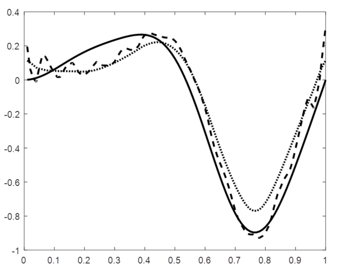
Figure 1: Behavior of the regression function and its estimates for $n=500$.

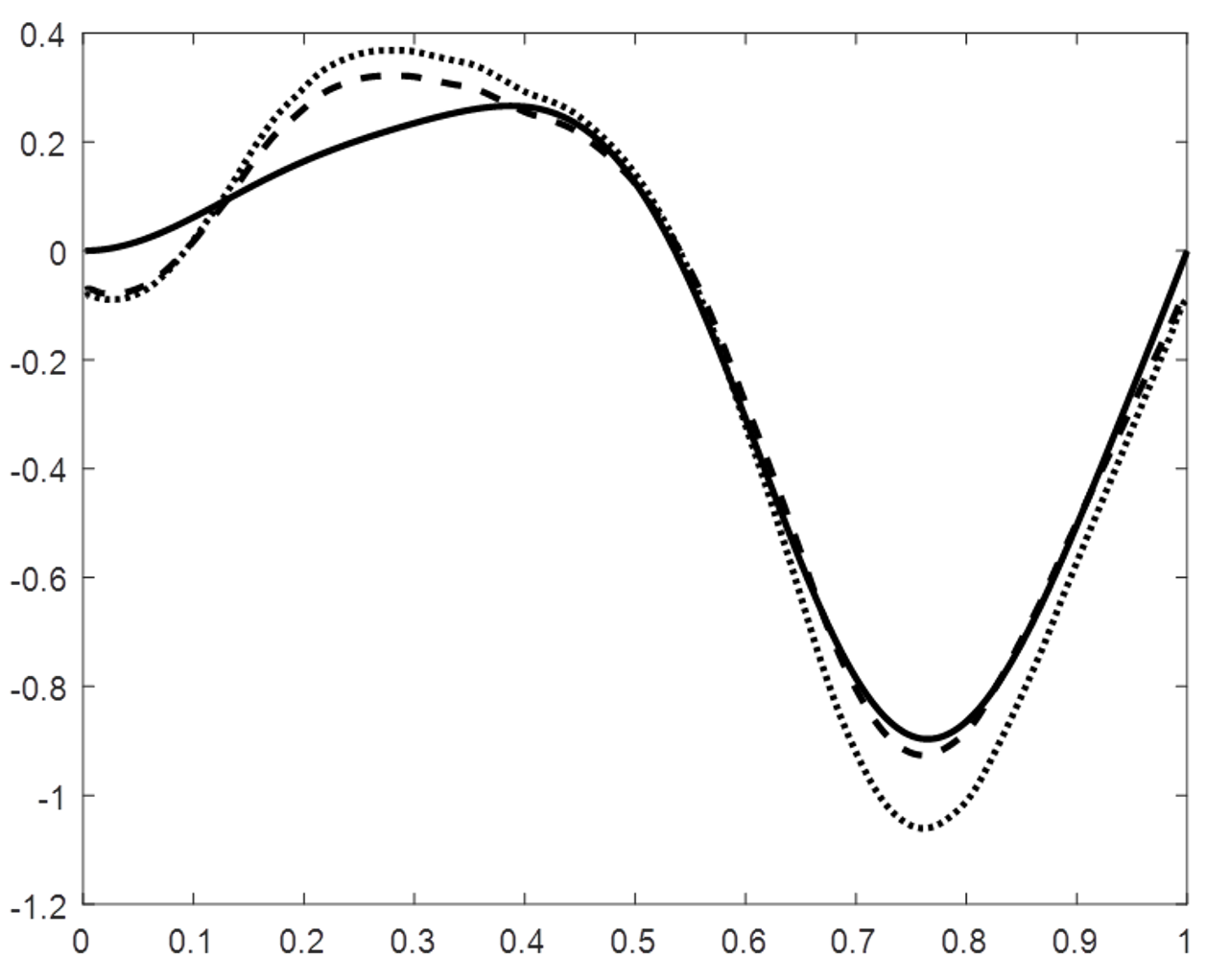
Figure 2: Behavior of the regression function and its estimates for $n=1000$.

Remark 6.1.

Figures 1–2 show the behavior of the procedures (3.8) and (4.6) depending on the values of observation periods $n$. The bold line is the function (6.1), the continuous line is the model selection procedure based on the least squares estimators $\widehat{S}$ and the dashed line is the improved model selection procedure $S^{*}$. From the Table 2 for the same $\gamma$ with various observations numbers $n$ we can conclude that theoretical result on the improvement effect (3.15) is confirmed by the numerical simulations. Moreover, for the proposed shrinkage procedure, Table 1 and Figures 1–2, we can conclude that the benefit is considerable for non large $n$.

7 Stochastic calculus for Ornstein-Uhlenbeck-Lévy process

In this section we study the process (2.1).

Proposition 7.1.

Let $f$ and $g$ be two nonrandom left continuous ${\mathbb{R}}_{\mathchoice{+}{+}{\lower 0.75346pt\hbox{$\scriptstyle+$}}{\lower 0.75346pt\hbox{$\scriptscriptstyle+$}}}\to{\mathbb{R}}$ functions with the finite right limits. Then for any $t>0$

$${\bf E}\,I_{\mathchoice{t}{t}{\lower 0.75346pt\hbox{$\scriptstyle t$}}{\lower 0.75346pt\hbox{$\scriptscriptstyle t$}}}(f)I_{\mathchoice{t}{t}{\lower 0.75346pt\hbox{$\scriptstyle t$}}{\lower 0.75346pt\hbox{$\scriptscriptstyle t$}}}(g)=\sigma_{\mathchoice{Q}{Q}{\lower 0.75346pt\hbox{$\scriptstyle Q$}}{\lower 0.75346pt\hbox{$\scriptscriptstyle Q$}}}\,\tau_{\mathchoice{t}{t}{\lower 0.75346pt\hbox{$\scriptstyle t$}}{\lower 0.75346pt\hbox{$\scriptscriptstyle t$}}}(f,g)\,,$$ (7.1)

where $\tau_{\mathchoice{t}{t}{\lower 0.75346pt\hbox{$\scriptstyle t$}}{\lower 0.75346pt\hbox{$\scriptscriptstyle t$}}}(f,g)=\int^{t}_{\mathchoice{0}{0}{\lower 0.75346pt\hbox{$\scriptstyle 0$}}{\lower 0.75346pt\hbox{$\scriptscriptstyle 0$}}}\left(f(s)g(s)+\check{\varepsilon}_{\mathchoice{s}{s}{\lower 0.75346pt\hbox{$\scriptstyle s$}}{\lower 0.75346pt\hbox{$\scriptscriptstyle s$}}}(f)g(s)+f(s)\check{\varepsilon}_{\mathchoice{s}{s}{\lower 0.75346pt\hbox{$\scriptstyle s$}}{\lower 0.75346pt\hbox{$\scriptscriptstyle s$}}}(g)\right)\,\mathrm{d}s$ and

$$\check{\varepsilon}_{\mathchoice{t}{t}{\lower 0.75346pt\hbox{$\scriptstyle t$}}{\lower 0.75346pt\hbox{$\scriptscriptstyle t$}}}(f)=a\int^{t}_{\mathchoice{0}{0}{\lower 0.75346pt\hbox{$\scriptstyle 0$}}{\lower 0.75346pt\hbox{$\scriptscriptstyle 0$}}}\,e^{a(t-s)}\,f(s)\left(\frac{1+e^{2as}}{2}\right)\,\mathrm{d}s\,.$$

Proof. Taking into account the definitions (3.7) and (2.1) we obtain through the Ito formula that

$$I_{\mathchoice{t}{t}{\lower 0.75346pt\hbox{$\scriptstyle t$}}{\lower 0.75346pt\hbox{$\scriptscriptstyle t$}}}(f)\,I_{\mathchoice{t}{t}{\lower 0.75346pt\hbox{$\scriptstyle t$}}{\lower 0.75346pt\hbox{$\scriptscriptstyle t$}}}(g)=\sigma_{\mathchoice{Q}{Q}{\lower 0.75346pt\hbox{$\scriptstyle Q$}}{\lower 0.75346pt\hbox{$\scriptscriptstyle Q$}}}\,\int^{t}_{\mathchoice{0}{0}{\lower 0.75346pt\hbox{$\scriptstyle 0$}}{\lower 0.75346pt\hbox{$\scriptscriptstyle 0$}}}\,f(s)g(s)\mathrm{d}s+a\int^{t}_{\mathchoice{0}{0}{\lower 0.75346pt\hbox{$\scriptstyle 0$}}{\lower 0.75346pt\hbox{$\scriptscriptstyle 0$}}}\Upsilon_{\mathchoice{s}{s}{\lower 0.75346pt\hbox{$\scriptstyle s$}}{\lower 0.75346pt\hbox{$\scriptscriptstyle s$}}}(f,g)\,\xi_{\mathchoice{t}{t}{\lower 0.75346pt\hbox{$\scriptstyle t$}}{\lower 0.75346pt\hbox{$\scriptscriptstyle t$}}}\mathrm{d}s+{\bf M}_{\mathchoice{t}{t}{\lower 0.75346pt\hbox{$\scriptstyle t$}}{\lower 0.75346pt\hbox{$\scriptscriptstyle t$}}}(f,g)\,,$$ (7.2)

where $\Upsilon_{\mathchoice{s}{s}{\lower 0.75346pt\hbox{$\scriptstyle s$}}{\lower 0.75346pt\hbox{$\scriptscriptstyle s$}}}(f,g)=f(s)I_{\mathchoice{s}{s}{\lower 0.75346pt\hbox{$\scriptstyle s$}}{\lower 0.75346pt\hbox{$\scriptscriptstyle s$}}}(g)+g(s)I_{\mathchoice{s}{s}{\lower 0.75346pt\hbox{$\scriptstyle s$}}{\lower 0.75346pt\hbox{$\scriptscriptstyle s$}}}(f)$,

$${\bf M}_{\mathchoice{t}{t}{\lower 0.75346pt\hbox{$\scriptstyle t$}}{\lower 0.75346pt\hbox{$\scriptscriptstyle t$}}}(f,g)=\int^{t}_{\mathchoice{0}{0}{\lower 0.75346pt\hbox{$\scriptstyle 0$}}{\lower 0.75346pt\hbox{$\scriptscriptstyle 0$}}}\,\Upsilon_{\mathchoice{s-}{s-}{\lower 0.75346pt\hbox{$\scriptstyle s-$}}{\lower 0.75346pt\hbox{$\scriptscriptstyle s-$}}}(f,g)\,\mathrm{d}u_{\mathchoice{s}{s}{\lower 0.75346pt\hbox{$\scriptstyle s$}}{\lower 0.75346pt\hbox{$\scriptscriptstyle s$}}}+\varrho^{2}_{\mathchoice{2}{2}{\lower 0.75346pt\hbox{$\scriptstyle 2$}}{\lower 0.75346pt\hbox{$\scriptscriptstyle 2$}}}\,\int^{t}_{\mathchoice{0}{0}{\lower 0.75346pt\hbox{$\scriptstyle 0$}}{\lower 0.75346pt\hbox{$\scriptscriptstyle 0$}}}f(s)\,g(s)\,\mathrm{d}m_{\mathchoice{s}{s}{\lower 0.75346pt\hbox{$\scriptstyle s$}}{\lower 0.75346pt\hbox{$\scriptscriptstyle s$}}}$$

and $m_{\mathchoice{t}{t}{\lower 0.75346pt\hbox{$\scriptstyle t$}}{\lower 0.75346pt\hbox{$\scriptscriptstyle t$}}}=x^{2}*(\mu-\widetilde{\mu})_{\mathchoice{t}{t}{\lower 0.75346pt\hbox{$\scriptstyle t$}}{\lower 0.75346pt\hbox{$\scriptscriptstyle t$}}}$. Moreover, using the Ito formula we obtain

$${\bf E}\,I^{2}_{\mathchoice{t}{t}{\lower 0.75346pt\hbox{$\scriptstyle t$}}{\lower 0.75346pt\hbox{$\scriptscriptstyle t$}}}(1)={\bf E}\,\xi^{2}_{\mathchoice{t}{t}{\lower 0.75346pt\hbox{$\scriptstyle t$}}{\lower 0.75346pt\hbox{$\scriptscriptstyle t$}}}=\sigma_{\mathchoice{Q}{Q}{\lower 0.75346pt\hbox{$\scriptstyle Q$}}{\lower 0.75346pt\hbox{$\scriptscriptstyle Q$}}}\,\frac{e^{2at}-1}{2a}\,.$$ (7.3)

Note now, that

$${\bf E}\,I^{2}_{\mathchoice{t}{t}{\lower 0.75346pt\hbox{$\scriptstyle t$}}{\lower 0.75346pt\hbox{$\scriptscriptstyle t$}}} ={\bf E}\left(a\int^{t}_{\mathchoice{0}{0}{\lower 0.75346pt\hbox{$\scriptstyle 0$}}{\lower 0.75346pt\hbox{$\scriptscriptstyle 0$}}}\,f(s)\xi_{\mathchoice{s}{s}{\lower 0.75346pt\hbox{$\scriptstyle s$}}{\lower 0.75346pt\hbox{$\scriptscriptstyle s$}}}\mathrm{d}s+\int^{t}_{\mathchoice{0}{0}{\lower 0.75346pt\hbox{$\scriptstyle 0$}}{\lower 0.75346pt\hbox{$\scriptscriptstyle 0$}}}\,f(s)\,\mathrm{d}u_{\mathchoice{s}{s}{\lower 0.75346pt\hbox{$\scriptstyle s$}}{\lower 0.75346pt\hbox{$\scriptscriptstyle s$}}}\right)^{2}$$

$$\leq 2a^{2}\,\int^{t}_{\mathchoice{0}{0}{\lower 0.75346pt\hbox{$\scriptstyle 0$}}{\lower 0.75346pt\hbox{$\scriptscriptstyle 0$}}}\,f^{2}(s)\mathrm{d}s\int^{t}_{\mathchoice{0}{0}{\lower 0.75346pt\hbox{$\scriptstyle 0$}}{\lower 0.75346pt\hbox{$\scriptscriptstyle 0$}}}\,{\bf E}\,\xi^{2}_{\mathchoice{s}{s}{\lower 0.75346pt\hbox{$\scriptstyle s$}}{\lower 0.75346pt\hbox{$\scriptscriptstyle s$}}}\mathrm{d}s+2\sigma_{\mathchoice{Q}{Q}{\lower 0.75346pt\hbox{$\scriptstyle Q$}}{\lower 0.75346pt\hbox{$\scriptscriptstyle Q$}}}\,\int^{t}_{\mathchoice{0}{0}{\lower 0.75346pt\hbox{$\scriptstyle 0$}}{\lower 0.75346pt\hbox{$\scriptscriptstyle 0$}}}\,f^{2}(s)\mathrm{d}s\,.$$

So, from here

$$\sup_{\mathchoice{0\leq t\leq n}{0\leq t\leq n}{\lower 0.75346pt\hbox{$\scriptstyle 0\leq t\leq n$}}{\lower 0.75346pt\hbox{$\scriptscriptstyle 0\leq t\leq n$}}}{\bf E}\,I^{2}_{\mathchoice{t}{t}{\lower 0.75346pt\hbox{$\scriptstyle t$}}{\lower 0.75346pt\hbox{$\scriptscriptstyle t$}}}(f)\leq 2\sigma_{\mathchoice{Q}{Q}{\lower 0.75346pt\hbox{$\scriptstyle Q$}}{\lower 0.75346pt\hbox{$\scriptscriptstyle Q$}}}\,(|a|+1)\,\int^{n}_{\mathchoice{0}{0}{\lower 0.75346pt\hbox{$\scriptstyle 0$}}{\lower 0.75346pt\hbox{$\scriptscriptstyle 0$}}}\,f^{2}(s)\mathrm{d}s<\infty\,.$$ (7.4)

This implies immediately that ${\bf E}\,{\bf M}_{\mathchoice{t}{t}{\lower 0.75346pt\hbox{$\scriptstyle t$}}{\lower 0.75346pt\hbox{$\scriptscriptstyle t$}}}(f,g)=0$. Using this in (7.2) yields

$${\bf E}\,I_{\mathchoice{t}{t}{\lower 0.75346pt\hbox{$\scriptstyle t$}}{\lower 0.75346pt\hbox{$\scriptscriptstyle t$}}}(f)\,I_{\mathchoice{t}{t}{\lower 0.75346pt\hbox{$\scriptstyle t$}}{\lower 0.75346pt\hbox{$\scriptscriptstyle t$}}}(g) =\sigma_{\mathchoice{Q}{Q}{\lower 0.75346pt\hbox{$\scriptstyle Q$}}{\lower 0.75346pt\hbox{$\scriptscriptstyle Q$}}}\,\int^{t}_{\mathchoice{0}{0}{\lower 0.75346pt\hbox{$\scriptstyle 0$}}{\lower 0.75346pt\hbox{$\scriptscriptstyle 0$}}}\,f(s)g(s)\mathrm{d}s$$

$$+a\int^{t}_{\mathchoice{0}{0}{\lower 0.75346pt\hbox{$\scriptstyle 0$}}{\lower 0.75346pt\hbox{$\scriptscriptstyle 0$}}}\left(f(s)\,{\bf E}\zeta_{\mathchoice{s}{s}{\lower 0.75346pt\hbox{$\scriptstyle s$}}{\lower 0.75346pt\hbox{$\scriptscriptstyle s$}}}(g)+g(s)\,{\bf E}\zeta_{\mathchoice{s}{s}{\lower 0.75346pt\hbox{$\scriptstyle s$}}{\lower 0.75346pt\hbox{$\scriptscriptstyle s$}}}(f)\right)\,\mathrm{d}s\,,$$ (7.5)

where $\zeta_{\mathchoice{t}{t}{\lower 0.75346pt\hbox{$\scriptstyle t$}}{\lower 0.75346pt\hbox{$\scriptscriptstyle t$}}}(f)=\xi_{\mathchoice{t}{t}{\lower 0.75346pt\hbox{$\scriptstyle t$}}{\lower 0.75346pt\hbox{$\scriptscriptstyle t$}}}\,I_{\mathchoice{t}{t}{\lower 0.75346pt\hbox{$\scriptstyle t$}}{\lower 0.75346pt\hbox{$\scriptscriptstyle t$}}}(f)=\,I_{\mathchoice{t}{t}{\lower 0.75346pt\hbox{$\scriptstyle t$}}{\lower 0.75346pt\hbox{$\scriptscriptstyle t$}}}(1)\,I_{\mathchoice{t}{t}{\lower 0.75346pt\hbox{$\scriptstyle t$}}{\lower 0.75346pt\hbox{$\scriptscriptstyle t$}}}(f)$. Therefore, putting $g=1$ in (7.5), we obtain that

$${\bf E}\,\zeta_{\mathchoice{t}{t}{\lower 0.75346pt\hbox{$\scriptstyle t$}}{\lower 0.75346pt\hbox{$\scriptscriptstyle t$}}}(f)=\sigma_{\mathchoice{Q}{Q}{\lower 0.75346pt\hbox{$\scriptstyle Q$}}{\lower 0.75346pt\hbox{$\scriptscriptstyle Q$}}}\,\int^{t}_{\mathchoice{0}{0}{\lower 0.75346pt\hbox{$\scriptstyle 0$}}{\lower 0.75346pt\hbox{$\scriptscriptstyle 0$}}}\,f(s)\mathrm{d}s+a\int^{t}_{\mathchoice{0}{0}{\lower 0.75346pt\hbox{$\scriptstyle 0$}}{\lower 0.75346pt\hbox{$\scriptscriptstyle 0$}}}\left(f(s){\bf E}\,\zeta_{\mathchoice{s}{s}{\lower 0.75346pt\hbox{$\scriptstyle s$}}{\lower 0.75346pt\hbox{$\scriptscriptstyle s$}}}(1)+{\bf E}\,\zeta_{\mathchoice{s}{s}{\lower 0.75346pt\hbox{$\scriptstyle s$}}{\lower 0.75346pt\hbox{$\scriptscriptstyle s$}}}(f)\right)\,\mathrm{d}s\,.$$

Taking into account here, that $\zeta_{\mathchoice{t}{t}{\lower 0.75346pt\hbox{$\scriptstyle t$}}{\lower 0.75346pt\hbox{$\scriptscriptstyle t$}}}(1)=\xi^{2}_{\mathchoice{t}{t}{\lower 0.75346pt\hbox{$\scriptstyle t$}}{\lower 0.75346pt\hbox{$\scriptscriptstyle t$}}}$, we obtain that

$${\bf E}\,\zeta_{\mathchoice{t}{t}{\lower 0.75346pt\hbox{$\scriptstyle t$}}{\lower 0.75346pt\hbox{$\scriptscriptstyle t$}}}(f)=\sigma_{\mathchoice{Q}{Q}{\lower 0.75346pt\hbox{$\scriptstyle Q$}}{\lower 0.75346pt\hbox{$\scriptscriptstyle Q$}}}\,\int^{t}\,e^{a(t-s)}f(s)\frac{1+e^{2as}}{2}\mathrm{d}s=\sigma_{\mathchoice{Q}{Q}{\lower 0.75346pt\hbox{$\scriptstyle Q$}}{\lower 0.75346pt\hbox{$\scriptscriptstyle Q$}}}\,\check{\varepsilon}_{\mathchoice{t}{t}{\lower 0.75346pt\hbox{$\scriptstyle t$}}{\lower 0.75346pt\hbox{$\scriptscriptstyle t$}}}(f)\,.$$

Therefore, using this in (7.5) we obtain (7.1).  ∎

Corollary 7.2.

For any cadlag function $f$ from ${\bf L}_{\mathchoice{2}{2}{\lower 0.75346pt\hbox{$\scriptstyle 2$}}{\lower 0.75346pt\hbox{$\scriptscriptstyle 2$}}}[0,n]$

$${\bf E}\,I^{2}_{\mathchoice{n}{n}{\lower 0.75346pt\hbox{$\scriptstyle n$}}{\lower 0.75346pt\hbox{$\scriptscriptstyle n$}}}(f)\leq 2\sigma_{\mathchoice{Q}{Q}{\lower 0.75346pt\hbox{$\scriptstyle Q$}}{\lower 0.75346pt\hbox{$\scriptscriptstyle Q$}}}\,\int^{n}_{\mathchoice{0}{0}{\lower 0.75346pt\hbox{$\scriptstyle 0$}}{\lower 0.75346pt\hbox{$\scriptscriptstyle 0$}}}\,f^{2}(s)\,\mathrm{d}s\,.$$ (7.6)

Proof. Indeed, putting $f=g$ in (7.1) we get

$${\bf E}\,I^{2}_{\mathchoice{n}{n}{\lower 0.75346pt\hbox{$\scriptstyle n$}}{\lower 0.75346pt\hbox{$\scriptscriptstyle n$}}}(f)=\sigma_{\mathchoice{Q}{Q}{\lower 0.75346pt\hbox{$\scriptstyle Q$}}{\lower 0.75346pt\hbox{$\scriptscriptstyle Q$}}}\,\int^{n}_{\mathchoice{0}{0}{\lower 0.75346pt\hbox{$\scriptstyle 0$}}{\lower 0.75346pt\hbox{$\scriptscriptstyle 0$}}}\,\left(f^{2}(t)+2\check{\varepsilon}_{\mathchoice{t}{t}{\lower 0.75346pt\hbox{$\scriptstyle t$}}{\lower 0.75346pt\hbox{$\scriptscriptstyle t$}}}(f)\,f(t)\right)\,\mathrm{d}t\,.$$

Moreover, note that

$$\int^{n}_{\mathchoice{0}{0}{\lower 0.75346pt\hbox{$\scriptstyle 0$}}{\lower 0.75346pt\hbox{$\scriptscriptstyle 0$}}}\,\check{\varepsilon}_{\mathchoice{t}{t}{\lower 0.75346pt\hbox{$\scriptstyle t$}}{\lower 0.75346pt\hbox{$\scriptscriptstyle t$}}}(f)\,f(t)\,\mathrm{d}t=a\int^{n}_{\mathchoice{0}{0}{\lower 0.75346pt\hbox{$\scriptstyle 0$}}{\lower 0.75346pt\hbox{$\scriptscriptstyle 0$}}}\,e^{ax}\,\int^{n}_{\mathchoice{x}{x}{\lower 0.75346pt\hbox{$\scriptstyle x$}}{\lower 0.75346pt\hbox{$\scriptscriptstyle x$}}}\,\left(f(t)f(t-x)\frac{1+e^{2a(t-x)}}{2}\right)\mathrm{d}t\,\mathrm{d}x\,.$$

By the Bunyakovskii–Cauchy–Schwarz inequality

$$\int^{n}_{\mathchoice{0}{0}{\lower 0.75346pt\hbox{$\scriptstyle 0$}}{\lower 0.75346pt\hbox{$\scriptscriptstyle 0$}}}\,\check{\varepsilon}_{\mathchoice{t}{t}{\lower 0.75346pt\hbox{$\scriptstyle t$}}{\lower 0.75346pt\hbox{$\scriptscriptstyle t$}}}(f)\,|f(t)|\,\mathrm{d}t\leq|a|\int^{n}_{\mathchoice{0}{0}{\lower 0.75346pt\hbox{$\scriptstyle 0$}}{\lower 0.75346pt\hbox{$\scriptscriptstyle 0$}}}\,e^{ax}\,\,\mathrm{d}x\,\int^{n}_{\mathchoice{0}{0}{\lower 0.75346pt\hbox{$\scriptstyle 0$}}{\lower 0.75346pt\hbox{$\scriptscriptstyle 0$}}}\,f^{2}(t)\,\mathrm{d}t\leq\int^{n}_{\mathchoice{0}{0}{\lower 0.75346pt\hbox{$\scriptstyle 0$}}{\lower 0.75346pt\hbox{$\scriptscriptstyle 0$}}}\,f^{2}(t)\,\mathrm{d}t\,.$$

This implies immediately upper bound (7.6). Hence Corollary 7.2.  ∎

Now we set

$$\widetilde{I}_{\mathchoice{t}{t}{\lower 0.75346pt\hbox{$\scriptstyle t$}}{\lower 0.75346pt\hbox{$\scriptscriptstyle t$}}}(f)=I^{2}_{\mathchoice{t}{t}{\lower 0.75346pt\hbox{$\scriptstyle t$}}{\lower 0.75346pt\hbox{$\scriptscriptstyle t$}}}(f)-{\bf E}\,I^{2}_{\mathchoice{t}{t}{\lower 0.75346pt\hbox{$\scriptstyle t$}}{\lower 0.75346pt\hbox{$\scriptscriptstyle t$}}}(f)\quad\mbox{and}\quad V_{\mathchoice{t}{t}{\lower 0.75346pt\hbox{$\scriptstyle t$}}{\lower 0.75346pt\hbox{$\scriptscriptstyle t$}}}(f)=\zeta_{\mathchoice{t}{t}{\lower 0.75346pt\hbox{$\scriptstyle t$}}{\lower 0.75346pt\hbox{$\scriptscriptstyle t$}}}(f)\,-{\bf E}\,\zeta_{\mathchoice{t}{t}{\lower 0.75346pt\hbox{$\scriptstyle t$}}{\lower 0.75346pt\hbox{$\scriptscriptstyle t$}}}(f)\,.$$ (7.7)

Using (7.2) with $f=g$ we can obtain that

$$\mathrm{d}\widetilde{I}_{\mathchoice{t}{t}{\lower 0.75346pt\hbox{$\scriptstyle t$}}{\lower 0.75346pt\hbox{$\scriptscriptstyle t$}}}(f)=2af(t)\,V_{\mathchoice{t}{t}{\lower 0.75346pt\hbox{$\scriptstyle t$}}{\lower 0.75346pt\hbox{$\scriptscriptstyle t$}}}(f)\mathrm{d}t+\mathrm{d}\widetilde{M}_{\mathchoice{t}{t}{\lower 0.75346pt\hbox{$\scriptstyle t$}}{\lower 0.75346pt\hbox{$\scriptscriptstyle t$}}}(f)\,,$$ (7.8)

where $\widetilde{M}_{\mathchoice{t}{t}{\lower 0.75346pt\hbox{$\scriptstyle t$}}{\lower 0.75346pt\hbox{$\scriptscriptstyle t$}}}(f)=M_{\mathchoice{t}{t}{\lower 0.75346pt\hbox{$\scriptstyle t$}}{\lower 0.75346pt\hbox{$\scriptscriptstyle t$}}}(f,f)$. To study this process we need to introduce the following functions

$$\check{\tau}_{\mathchoice{t}{t}{\lower 0.75346pt\hbox{$\scriptstyle t$}}{\lower 0.75346pt\hbox{$\scriptscriptstyle t$}}}(f,g)=f(t)g(t)\tau_{\mathchoice{t}{t}{\lower 0.75346pt\hbox{$\scriptstyle t$}}{\lower 0.75346pt\hbox{$\scriptscriptstyle t$}}}(1,1)+f(t)\tau_{\mathchoice{t}{t}{\lower 0.75346pt\hbox{$\scriptstyle t$}}{\lower 0.75346pt\hbox{$\scriptscriptstyle t$}}}(1,g)+g(t)\tau_{\mathchoice{t}{t}{\lower 0.75346pt\hbox{$\scriptstyle t$}}{\lower 0.75346pt\hbox{$\scriptscriptstyle t$}}}(1,f)+\tau_{\mathchoice{t}{t}{\lower 0.75346pt\hbox{$\scriptstyle t$}}{\lower 0.75346pt\hbox{$\scriptscriptstyle t$}}}(f,g)$$ (7.9)

and

$$A_{\mathchoice{t}{t}{\lower 0.75346pt\hbox{$\scriptstyle t$}}{\lower 0.75346pt\hbox{$\scriptscriptstyle t$}}}(f)=\int^{t}_{\mathchoice{0}{0}{\lower 0.75346pt\hbox{$\scriptstyle 0$}}{\lower 0.75346pt\hbox{$\scriptscriptstyle 0$}}}e^{3a(t-s)}f(s)\upsilon(s)\mathrm{d}s+2\,\sigma_{\mathchoice{Q}{Q}{\lower 0.75346pt\hbox{$\scriptstyle Q$}}{\lower 0.75346pt\hbox{$\scriptscriptstyle Q$}}}^{2}\,\int^{t}_{\mathchoice{0}{0}{\lower 0.75346pt\hbox{$\scriptstyle 0$}}{\lower 0.75346pt\hbox{$\scriptscriptstyle 0$}}}e^{3a(t-s)}\check{\varepsilon}_{\mathchoice{s}{s}{\lower 0.75346pt\hbox{$\scriptstyle s$}}{\lower 0.75346pt\hbox{$\scriptscriptstyle s$}}}(f)\mathrm{d}s\,,$$ (7.10)

where $\upsilon(s)=a^{2}{\bf E}\,\widetilde{\xi}^{2}_{\mathchoice{s}{s}{\lower 0.75346pt\hbox{$\scriptstyle s$}}{\lower 0.75346pt\hbox{$\scriptscriptstyle s$}}}+\sigma_{\mathchoice{Q}{Q}{\lower 0.75346pt\hbox{$\scriptstyle Q$}}{\lower 0.75346pt\hbox{$\scriptscriptstyle Q$}}}^{2}\left(e^{2as}-1\right)+a\check{\varrho}_{\mathchoice{2}{2}{\lower 0.75346pt\hbox{$\scriptstyle 2$}}{\lower 0.75346pt\hbox{$\scriptscriptstyle 2$}}}$, $\widetilde{\xi}_{\mathchoice{s}{s}{\lower 0.75346pt\hbox{$\scriptstyle s$}}{\lower 0.75346pt\hbox{$\scriptscriptstyle s$}}}=\xi^{2}_{\mathchoice{s}{s}{\lower 0.75346pt\hbox{$\scriptstyle s$}}{\lower 0.75346pt\hbox{$\scriptscriptstyle s$}}}-{\bf E}\,\xi^{2}_{\mathchoice{s}{s}{\lower 0.75346pt\hbox{$\scriptstyle s$}}{\lower 0.75346pt\hbox{$\scriptscriptstyle s$}}}$ and $\check{\varrho}_{\mathchoice{2}{2}{\lower 0.75346pt\hbox{$\scriptstyle 2$}}{\lower 0.75346pt\hbox{$\scriptscriptstyle 2$}}}=\varrho^{4}_{\mathchoice{2}{2}{\lower 0.75346pt\hbox{$\scriptstyle 2$}}{\lower 0.75346pt\hbox{$\scriptscriptstyle 2$}}}\,\Pi(x^{4})$.

Proposition 7.3.

For any left continuous functions with finite right limits $f$ and $g$

$${\bf E}\,V_{\mathchoice{t}{t}{\lower 0.75346pt\hbox{$\scriptstyle t$}}{\lower 0.75346pt\hbox{$\scriptscriptstyle t$}}}(f)V_{\mathchoice{t}{t}{\lower 0.75346pt\hbox{$\scriptstyle t$}}{\lower 0.75346pt\hbox{$\scriptscriptstyle t$}}}(g)=\int^{t}_{\mathchoice{0}{0}{\lower 0.75346pt\hbox{$\scriptstyle 0$}}{\lower 0.75346pt\hbox{$\scriptscriptstyle 0$}}}\,e^{2a(t-s)}\,H_{\mathchoice{s}{s}{\lower 0.75346pt\hbox{$\scriptstyle s$}}{\lower 0.75346pt\hbox{$\scriptscriptstyle s$}}}(f,g)\,\mathrm{d}s$$ (7.11)

where $H_{\mathchoice{t}{t}{\lower 0.75346pt\hbox{$\scriptstyle t$}}{\lower 0.75346pt\hbox{$\scriptscriptstyle t$}}}(f,g)=g(t)A_{\mathchoice{t}{t}{\lower 0.75346pt\hbox{$\scriptstyle t$}}{\lower 0.75346pt\hbox{$\scriptscriptstyle t$}}}(f)+f(t)A_{\mathchoice{t}{t}{\lower 0.75346pt\hbox{$\scriptstyle t$}}{\lower 0.75346pt\hbox{$\scriptscriptstyle t$}}}(g)+\sigma_{\mathchoice{Q}{Q}{\lower 0.75346pt\hbox{$\scriptstyle Q$}}{\lower 0.75346pt\hbox{$\scriptscriptstyle Q$}}}^{2}\check{\tau}_{\mathchoice{t}{t}{\lower 0.75346pt\hbox{$\scriptstyle t$}}{\lower 0.75346pt\hbox{$\scriptscriptstyle t$}}}(f,g)+\check{\varrho}_{\mathchoice{2}{2}{\lower 0.75346pt\hbox{$\scriptstyle 2$}}{\lower 0.75346pt\hbox{$\scriptscriptstyle 2$}}}\,f(t)g(t)$.

Proof. Applying again (7.2) with $g=1$ yields

$$\mathrm{d}V_{\mathchoice{t}{t}{\lower 0.75346pt\hbox{$\scriptstyle t$}}{\lower 0.75346pt\hbox{$\scriptscriptstyle t$}}}(f)=aV_{\mathchoice{t}{t}{\lower 0.75346pt\hbox{$\scriptstyle t$}}{\lower 0.75346pt\hbox{$\scriptscriptstyle t$}}}(f)\mathrm{d}t+a\,f(t)\,\widetilde{I}_{\mathchoice{t}{t}{\lower 0.75346pt\hbox{$\scriptstyle t$}}{\lower 0.75346pt\hbox{$\scriptscriptstyle t$}}}(1)\mathrm{d}t+\mathrm{d}\,L_{\mathchoice{t}{t}{\lower 0.75346pt\hbox{$\scriptstyle t$}}{\lower 0.75346pt\hbox{$\scriptscriptstyle t$}}}(f)\,,$$ (7.12)

where $L_{\mathchoice{t}{t}{\lower 0.75346pt\hbox{$\scriptstyle t$}}{\lower 0.75346pt\hbox{$\scriptscriptstyle t$}}}(f)=\int^{t}_{\mathchoice{0}{0}{\lower 0.75346pt\hbox{$\scriptstyle 0$}}{\lower 0.75346pt\hbox{$\scriptscriptstyle 0$}}}\,\check{I}_{\mathchoice{s-}{s-}{\lower 0.75346pt\hbox{$\scriptstyle s-$}}{\lower 0.75346pt\hbox{$\scriptscriptstyle s-$}}}(f)\mathrm{d}u_{\mathchoice{s}{s}{\lower 0.75346pt\hbox{$\scriptstyle s$}}{\lower 0.75346pt\hbox{$\scriptscriptstyle s$}}}+\varrho^{2}_{\mathchoice{2}{2}{\lower 0.75346pt\hbox{$\scriptstyle 2$}}{\lower 0.75346pt\hbox{$\scriptscriptstyle 2$}}}\int^{t}_{\mathchoice{0}{0}{\lower 0.75346pt\hbox{$\scriptstyle 0$}}{\lower 0.75346pt\hbox{$\scriptscriptstyle 0$}}}\,f(s)\mathrm{d}m_{\mathchoice{s}{s}{\lower 0.75346pt\hbox{$\scriptstyle s$}}{\lower 0.75346pt\hbox{$\scriptscriptstyle s$}}}$ and $\check{I}_{\mathchoice{s}{s}{\lower 0.75346pt\hbox{$\scriptstyle s$}}{\lower 0.75346pt\hbox{$\scriptscriptstyle s$}}}(f)=f(s)\xi_{\mathchoice{s}{s}{\lower 0.75346pt\hbox{$\scriptstyle s$}}{\lower 0.75346pt\hbox{$\scriptscriptstyle s$}}}+I_{\mathchoice{s}{s}{\lower 0.75346pt\hbox{$\scriptstyle s$}}{\lower 0.75346pt\hbox{$\scriptscriptstyle s$}}}(f)$. By the Ito formula we get

$$\mathrm{d}V_{\mathchoice{t}{t}{\lower 0.75346pt\hbox{$\scriptstyle t$}}{\lower 0.75346pt\hbox{$\scriptscriptstyle t$}}}(f)V_{\mathchoice{t}{t}{\lower 0.75346pt\hbox{$\scriptstyle t$}}{\lower 0.75346pt\hbox{$\scriptscriptstyle t$}}}(g) =2aV_{\mathchoice{t}{t}{\lower 0.75346pt\hbox{$\scriptstyle t$}}{\lower 0.75346pt\hbox{$\scriptscriptstyle t$}}}(f)\,V_{\mathchoice{t}{t}{\lower 0.75346pt\hbox{$\scriptstyle t$}}{\lower 0.75346pt\hbox{$\scriptscriptstyle t$}}}(g)\mathrm{d}t+a\left(g(t)V_{\mathchoice{t}{t}{\lower 0.75346pt\hbox{$\scriptstyle t$}}{\lower 0.75346pt\hbox{$\scriptscriptstyle t$}}}(f)+f(t)V_{\mathchoice{t}{t}{\lower 0.75346pt\hbox{$\scriptstyle t$}}{\lower 0.75346pt\hbox{$\scriptscriptstyle t$}}}(g)\right)\,\widetilde{I}_{\mathchoice{t}{t}{\lower 0.75346pt\hbox{$\scriptstyle t$}}{\lower 0.75346pt\hbox{$\scriptscriptstyle t$}}}(1)\mathrm{d}t$$

$$+\mathrm{d}\,[L(f)\,,\,L(g)]_{\mathchoice{t}{t}{\lower 0.75346pt\hbox{$\scriptstyle t$}}{\lower 0.75346pt\hbox{$\scriptscriptstyle t$}}}+V_{\mathchoice{t-}{t-}{\lower 0.75346pt\hbox{$\scriptstyle t-$}}{\lower 0.75346pt\hbox{$\scriptscriptstyle t-$}}}(f)\mathrm{d}L_{\mathchoice{t}{t}{\lower 0.75346pt\hbox{$\scriptstyle t$}}{\lower 0.75346pt\hbox{$\scriptscriptstyle t$}}}(g)+V_{\mathchoice{t-}{t-}{\lower 0.75346pt\hbox{$\scriptstyle t-$}}{\lower 0.75346pt\hbox{$\scriptscriptstyle t-$}}}(g)\mathrm{d}L_{\mathchoice{t}{t}{\lower 0.75346pt\hbox{$\scriptstyle t$}}{\lower 0.75346pt\hbox{$\scriptscriptstyle t$}}}(f)\,.$$

Now from Lemma A.2 we obtain that

$$\mathrm{d}{\bf E}\,V_{\mathchoice{t}{t}{\lower 0.75346pt\hbox{$\scriptstyle t$}}{\lower 0.75346pt\hbox{$\scriptscriptstyle t$}}}(f)V_{\mathchoice{t}{t}{\lower 0.75346pt\hbox{$\scriptstyle t$}}{\lower 0.75346pt\hbox{$\scriptscriptstyle t$}}}(g) =2a{\bf E}\,V_{\mathchoice{t}{t}{\lower 0.75346pt\hbox{$\scriptstyle t$}}{\lower 0.75346pt\hbox{$\scriptscriptstyle t$}}}(f)\,V_{\mathchoice{t}{t}{\lower 0.75346pt\hbox{$\scriptstyle t$}}{\lower 0.75346pt\hbox{$\scriptscriptstyle t$}}}(g)\mathrm{d}t+\left(g(t)A_{\mathchoice{t}{t}{\lower 0.75346pt\hbox{$\scriptstyle t$}}{\lower 0.75346pt\hbox{$\scriptscriptstyle t$}}}(f)+f(t)A_{\mathchoice{t}{t}{\lower 0.75346pt\hbox{$\scriptstyle t$}}{\lower 0.75346pt\hbox{$\scriptscriptstyle t$}}}(g)\right)\,\mathrm{d}t$$

$$+\mathrm{d}\,{\bf E}\,[L(f)\,,\,L(g)]_{\mathchoice{t}{t}{\lower 0.75346pt\hbox{$\scriptstyle t$}}{\lower 0.75346pt\hbox{$\scriptscriptstyle t$}}}\,,$$ (7.13)

where $A_{\mathchoice{t}{t}{\lower 0.75346pt\hbox{$\scriptstyle t$}}{\lower 0.75346pt\hbox{$\scriptscriptstyle t$}}}(f)=a{\bf E}\,V_{\mathchoice{t}{t}{\lower 0.75346pt\hbox{$\scriptstyle t$}}{\lower 0.75346pt\hbox{$\scriptscriptstyle t$}}}(f)\,\widetilde{I}_{\mathchoice{t}{t}{\lower 0.75346pt\hbox{$\scriptstyle t$}}{\lower 0.75346pt\hbox{$\scriptscriptstyle t$}}}(1)=a{\bf E}\,V_{\mathchoice{t}{t}{\lower 0.75346pt\hbox{$\scriptstyle t$}}{\lower 0.75346pt\hbox{$\scriptscriptstyle t$}}}(f)\,V_{\mathchoice{t}{t}{\lower 0.75346pt\hbox{$\scriptstyle t$}}{\lower 0.75346pt\hbox{$\scriptscriptstyle t$}}}(1)$. Note that ${\bf E}\,\check{I}_{\mathchoice{s}{s}{\lower 0.75346pt\hbox{$\scriptstyle s$}}{\lower 0.75346pt\hbox{$\scriptscriptstyle s$}}}(f)\check{I}_{\mathchoice{s}{s}{\lower 0.75346pt\hbox{$\scriptstyle s$}}{\lower 0.75346pt\hbox{$\scriptscriptstyle s$}}}(g)=\sigma_{\mathchoice{Q}{Q}{\lower 0.75346pt\hbox{$\scriptstyle Q$}}{\lower 0.75346pt\hbox{$\scriptscriptstyle Q$}}}\check{\tau}_{\mathchoice{s}{s}{\lower 0.75346pt\hbox{$\scriptstyle s$}}{\lower 0.75346pt\hbox{$\scriptscriptstyle s$}}}(f,g)$ and

$${\bf E}\,[L(f)\,,\,L(g)]_{\mathchoice{t}{t}{\lower 0.75346pt\hbox{$\scriptstyle t$}}{\lower 0.75346pt\hbox{$\scriptscriptstyle t$}}} =\varrho^{2}_{\mathchoice{1}{1}{\lower 0.75346pt\hbox{$\scriptstyle 1$}}{\lower 0.75346pt\hbox{$\scriptscriptstyle 1$}}}\,\int^{t}_{\mathchoice{0}{0}{\lower 0.75346pt\hbox{$\scriptstyle 0$}}{\lower 0.75346pt\hbox{$\scriptscriptstyle 0$}}}\,{\bf E}\,\check{I}_{\mathchoice{s}{s}{\lower 0.75346pt\hbox{$\scriptstyle s$}}{\lower 0.75346pt\hbox{$\scriptscriptstyle s$}}}(f)\,\check{I}_{\mathchoice{s}{s}{\lower 0.75346pt\hbox{$\scriptstyle s$}}{\lower 0.75346pt\hbox{$\scriptscriptstyle s$}}}(g)\,\mathrm{d}s+{\bf E}\,\sum_{\mathchoice{0\leq s\leq t}{0\leq s\leq t}{\lower 0.75346pt\hbox{$\scriptstyle 0\leq s\leq t$}}{\lower 0.75346pt\hbox{$\scriptscriptstyle 0\leq s\leq t$}}}\,\Delta\,L_{\mathchoice{s}{s}{\lower 0.75346pt\hbox{$\scriptstyle s$}}{\lower 0.75346pt\hbox{$\scriptscriptstyle s$}}}(f)\Delta\,L_{\mathchoice{s}{s}{\lower 0.75346pt\hbox{$\scriptstyle s$}}{\lower 0.75346pt\hbox{$\scriptscriptstyle s$}}}(g)$$

$$=\sigma_{\mathchoice{Q}{Q}{\lower 0.75346pt\hbox{$\scriptstyle Q$}}{\lower 0.75346pt\hbox{$\scriptscriptstyle Q$}}}^{2}\,\int^{t}_{\mathchoice{0}{0}{\lower 0.75346pt\hbox{$\scriptstyle 0$}}{\lower 0.75346pt\hbox{$\scriptscriptstyle 0$}}}\,\check{\tau}_{\mathchoice{s}{s}{\lower 0.75346pt\hbox{$\scriptstyle s$}}{\lower 0.75346pt\hbox{$\scriptscriptstyle s$}}}(f,g)\,\mathrm{d}s+\check{\varrho}_{\mathchoice{2}{2}{\lower 0.75346pt\hbox{$\scriptstyle 2$}}{\lower 0.75346pt\hbox{$\scriptscriptstyle 2$}}}\,\int^{t}_{\mathchoice{0}{0}{\lower 0.75346pt\hbox{$\scriptstyle 0$}}{\lower 0.75346pt\hbox{$\scriptscriptstyle 0$}}}\,f(s)g(s)\mathrm{d}s\,.$$

To find the function $A_{\mathchoice{t}{t}{\lower 0.75346pt\hbox{$\scriptstyle t$}}{\lower 0.75346pt\hbox{$\scriptscriptstyle t$}}}(f)$ we put $g=1$ in (7.13). Taking into account that $A_{\mathchoice{t}{t}{\lower 0.75346pt\hbox{$\scriptstyle t$}}{\lower 0.75346pt\hbox{$\scriptscriptstyle t$}}}(1)=\widetilde{I}^{2}_{\mathchoice{t}{t}{\lower 0.75346pt\hbox{$\scriptstyle t$}}{\lower 0.75346pt\hbox{$\scriptscriptstyle t$}}}=\widetilde{\xi}^{2}_{\mathchoice{t}{t}{\lower 0.75346pt\hbox{$\scriptstyle t$}}{\lower 0.75346pt\hbox{$\scriptscriptstyle t$}}}$ we get

$${\bf E}\,V_{\mathchoice{t}{t}{\lower 0.75346pt\hbox{$\scriptstyle t$}}{\lower 0.75346pt\hbox{$\scriptscriptstyle t$}}}(f)V_{\mathchoice{t}{t}{\lower 0.75346pt\hbox{$\scriptstyle t$}}{\lower 0.75346pt\hbox{$\scriptscriptstyle t$}}}(1)=\int^{t}_{\mathchoice{0}{0}{\lower 0.75346pt\hbox{$\scriptstyle 0$}}{\lower 0.75346pt\hbox{$\scriptscriptstyle 0$}}}\,e^{3a(t-s)}\,\left(a\,f(s)\,{\bf E}\,\widetilde{\xi}^{2}_{\mathchoice{s}{s}{\lower 0.75346pt\hbox{$\scriptstyle s$}}{\lower 0.75346pt\hbox{$\scriptscriptstyle s$}}}+\sigma_{\mathchoice{Q}{Q}{\lower 0.75346pt\hbox{$\scriptstyle Q$}}{\lower 0.75346pt\hbox{$\scriptscriptstyle Q$}}}^{2}\,\check{\tau}_{\mathchoice{s}{s}{\lower 0.75346pt\hbox{$\scriptstyle s$}}{\lower 0.75346pt\hbox{$\scriptscriptstyle s$}}}(f,1)+\check{\varrho}_{\mathchoice{2}{2}{\lower 0.75346pt\hbox{$\scriptstyle 2$}}{\lower 0.75346pt\hbox{$\scriptscriptstyle 2$}}}\,f(s)\right)\mathrm{d}s\,.$$

Using here that

$$a\tau_{\mathchoice{t}{t}{\lower 0.75346pt\hbox{$\scriptstyle t$}}{\lower 0.75346pt\hbox{$\scriptscriptstyle t$}}}(1,1)=(e^{2at}-1)/2\quad\mbox{and}\quad a\,\tau_{\mathchoice{t}{t}{\lower 0.75346pt\hbox{$\scriptstyle t$}}{\lower 0.75346pt\hbox{$\scriptscriptstyle t$}}}(1,f)=\check{\varepsilon}_{\mathchoice{t}{t}{\lower 0.75346pt\hbox{$\scriptstyle t$}}{\lower 0.75346pt\hbox{$\scriptscriptstyle t$}}}(f)\,,$$ (7.14)

we obtain the representation (7.10). Hence Proposition 7.3.  ∎

Proposition 7.4.

For any left continuous function $f$ with finite right limits

$${\bf E}\,\widetilde{I}_{\mathchoice{t}{t}{\lower 0.75346pt\hbox{$\scriptstyle t$}}{\lower 0.75346pt\hbox{$\scriptscriptstyle t$}}}(f)\,\widetilde{I}_{\mathchoice{t}{t}{\lower 0.75346pt\hbox{$\scriptstyle t$}}{\lower 0.75346pt\hbox{$\scriptscriptstyle t$}}}(1)=\int^{t}_{\mathchoice{0}{0}{\lower 0.75346pt\hbox{$\scriptstyle 0$}}{\lower 0.75346pt\hbox{$\scriptscriptstyle 0$}}}\,e^{2a(t-s)}\,\widetilde{\varkappa}_{\mathchoice{s}{s}{\lower 0.75346pt\hbox{$\scriptstyle s$}}{\lower 0.75346pt\hbox{$\scriptscriptstyle s$}}}(f)\,\mathrm{d}s\,,$$ (7.15)

where $\widetilde{\varkappa}_{\mathchoice{s}{s}{\lower 0.75346pt\hbox{$\scriptstyle s$}}{\lower 0.75346pt\hbox{$\scriptscriptstyle s$}}}(f)=2f(s)\,A_{\mathchoice{s}{s}{\lower 0.75346pt\hbox{$\scriptstyle s$}}{\lower 0.75346pt\hbox{$\scriptscriptstyle s$}}}(f)\,+4\sigma_{\mathchoice{Q}{Q}{\lower 0.75346pt\hbox{$\scriptstyle Q$}}{\lower 0.75346pt\hbox{$\scriptscriptstyle Q$}}}^{2}\,f(s)\tau_{\mathchoice{s}{s}{\lower 0.75346pt\hbox{$\scriptstyle s$}}{\lower 0.75346pt\hbox{$\scriptscriptstyle s$}}}(f,1)+\check{\varrho}_{\mathchoice{2}{2}{\lower 0.75346pt\hbox{$\scriptstyle 2$}}{\lower 0.75346pt\hbox{$\scriptscriptstyle 2$}}}\,f^{2}(s)$.

Proof. Using the Ito formula and Lemma A.2 we obtain that for any bounded nonrandom functions $f$ and $g$

$$\mathrm{d}{\bf E}\,\widetilde{I}_{\mathchoice{t}{t}{\lower 0.75346pt\hbox{$\scriptstyle t$}}{\lower 0.75346pt\hbox{$\scriptscriptstyle t$}}}(f)\,V_{\mathchoice{t}{t}{\lower 0.75346pt\hbox{$\scriptstyle t$}}{\lower 0.75346pt\hbox{$\scriptscriptstyle t$}}}(g) =a{\bf E}\,\widetilde{I}_{\mathchoice{t}{t}{\lower 0.75346pt\hbox{$\scriptstyle t$}}{\lower 0.75346pt\hbox{$\scriptscriptstyle t$}}}(f)\,V_{\mathchoice{t}{t}{\lower 0.75346pt\hbox{$\scriptstyle t$}}{\lower 0.75346pt\hbox{$\scriptscriptstyle t$}}}(g)\,\mathrm{d}t+2af(t){\bf E}\,V_{\mathchoice{t}{t}{\lower 0.75346pt\hbox{$\scriptstyle t$}}{\lower 0.75346pt\hbox{$\scriptscriptstyle t$}}}(f)\,V_{\mathchoice{t}{t}{\lower 0.75346pt\hbox{$\scriptstyle t$}}{\lower 0.75346pt\hbox{$\scriptscriptstyle t$}}}(g)\,\mathrm{d}t$$

$$+a\,g(t)\,{\bf E}\,\widetilde{I}_{\mathchoice{t}{t}{\lower 0.75346pt\hbox{$\scriptstyle t$}}{\lower 0.75346pt\hbox{$\scriptscriptstyle t$}}}(f)\,\widetilde{I}_{\mathchoice{t}{t}{\lower 0.75346pt\hbox{$\scriptstyle t$}}{\lower 0.75346pt\hbox{$\scriptscriptstyle t$}}}(1)\mathrm{d}t+\mathrm{d}{\bf E}\,[\widetilde{M}(f)\,,\,L(g)]_{\mathchoice{t}{t}{\lower 0.75346pt\hbox{$\scriptstyle t$}}{\lower 0.75346pt\hbox{$\scriptscriptstyle t$}}}\,.$$ (7.16)

Putting here $g=1$ and taking into account that $V_{\mathchoice{t}{t}{\lower 0.75346pt\hbox{$\scriptstyle t$}}{\lower 0.75346pt\hbox{$\scriptscriptstyle t$}}}(1)=\widetilde{I}_{\mathchoice{t}{t}{\lower 0.75346pt\hbox{$\scriptstyle t$}}{\lower 0.75346pt\hbox{$\scriptscriptstyle t$}}}(1)$, we obtain that

$$\mathrm{d}{\bf E}\,\widetilde{I}_{\mathchoice{t}{t}{\lower 0.75346pt\hbox{$\scriptstyle t$}}{\lower 0.75346pt\hbox{$\scriptscriptstyle t$}}}(f)\,V_{\mathchoice{t}{t}{\lower 0.75346pt\hbox{$\scriptstyle t$}}{\lower 0.75346pt\hbox{$\scriptscriptstyle t$}}}(1) =2a{\bf E}\,\widetilde{I}_{\mathchoice{t}{t}{\lower 0.75346pt\hbox{$\scriptstyle t$}}{\lower 0.75346pt\hbox{$\scriptscriptstyle t$}}}(f)\,V_{\mathchoice{t}{t}{\lower 0.75346pt\hbox{$\scriptstyle t$}}{\lower 0.75346pt\hbox{$\scriptscriptstyle t$}}}(1)\,\mathrm{d}t+2af(t){\bf E}\,V_{\mathchoice{t}{t}{\lower 0.75346pt\hbox{$\scriptstyle t$}}{\lower 0.75346pt\hbox{$\scriptscriptstyle t$}}}(f)\,V_{\mathchoice{t}{t}{\lower 0.75346pt\hbox{$\scriptstyle t$}}{\lower 0.75346pt\hbox{$\scriptscriptstyle t$}}}(1)\,\mathrm{d}t$$

$$+\mathrm{d}{\bf E}\,[\widetilde{M}(f)\,,\,L(1)]_{\mathchoice{t}{t}{\lower 0.75346pt\hbox{$\scriptstyle t$}}{\lower 0.75346pt\hbox{$\scriptscriptstyle t$}}}\,.$$

By the direct calculation we find

$${\bf E}\,[\widetilde{M}(f)\,,\,L(1)]_{\mathchoice{t}{t}{\lower 0.75346pt\hbox{$\scriptstyle t$}}{\lower 0.75346pt\hbox{$\scriptscriptstyle t$}}}=\int^{t}_{\mathchoice{0}{0}{\lower 0.75346pt\hbox{$\scriptstyle 0$}}{\lower 0.75346pt\hbox{$\scriptscriptstyle 0$}}}\,\check{A}_{\mathchoice{s}{s}{\lower 0.75346pt\hbox{$\scriptstyle s$}}{\lower 0.75346pt\hbox{$\scriptscriptstyle s$}}}(f)\mathrm{d}s\,.$$

So, we get (7.15) and this proposition.  ∎

Further we need the following correlation measures for two integrated $[0,+\infty)\to{\mathbb{R}}$ functions $f$ and $g$

$$\varpi_{\mathchoice{n}{n}{\lower 0.75346pt\hbox{$\scriptstyle n$}}{\lower 0.75346pt\hbox{$\scriptscriptstyle n$}}}(f,g)=\max_{\mathchoice{0\leq v+t\leq n}{0\leq v+t\leq n}{\lower 0.75346pt\hbox{$\scriptstyle 0\leq v+t\leq n$}}{\lower 0.75346pt\hbox{$\scriptscriptstyle 0\leq v+t\leq n$}}}\,\left(\left|\int^{t}_{\mathchoice{0}{0}{\lower 0.75346pt\hbox{$\scriptstyle 0$}}{\lower 0.75346pt\hbox{$\scriptscriptstyle 0$}}}f(u+v)g(u)\mathrm{d}u\right|+\left|\int^{t}_{\mathchoice{0}{0}{\lower 0.75346pt\hbox{$\scriptstyle 0$}}{\lower 0.75346pt\hbox{$\scriptscriptstyle 0$}}}g(u+v)f(u)\mathrm{d}u\right|\right)$$ (7.17)

For any bounded $[0,\infty)\to{\mathbb{R}}$ function $f$ we introduce the following uniform norm

$$\|f\|_{\mathchoice{*,n}{*,n}{\lower 0.75346pt\hbox{$\scriptstyle*,n$}}{\lower 0.75346pt\hbox{$\scriptscriptstyle*,n$}}}=\sup_{\mathchoice{0\leq t\leq n}{0\leq t\leq n}{\lower 0.75346pt\hbox{$\scriptstyle 0\leq t\leq n$}}{\lower 0.75346pt\hbox{$\scriptscriptstyle 0\leq t\leq n$}}}|f(t)|\,.$$

Proposition 7.5.

Let $f$ and $g$ be two left continuous bounded by $\phi_{\mathchoice{*}{*}{\lower 0.75346pt\hbox{$\scriptstyle*$}}{\lower 0.75346pt\hbox{$\scriptscriptstyle*$}}}$ functions with finite right limits, i.e. $\|f\|_{\mathchoice{*,n}{*,n}{\lower 0.75346pt\hbox{$\scriptstyle*,n$}}{\lower 0.75346pt\hbox{$\scriptscriptstyle*,n$}}}\leq\phi_{\mathchoice{*}{*}{\lower 0.75346pt\hbox{$\scriptstyle*$}}{\lower 0.75346pt\hbox{$\scriptscriptstyle*$}}}$ and $\|g\|_{\mathchoice{*,n}{*,n}{\lower 0.75346pt\hbox{$\scriptstyle*,n$}}{\lower 0.75346pt\hbox{$\scriptscriptstyle*,n$}}}\leq\phi_{\mathchoice{*}{*}{\lower 0.75346pt\hbox{$\scriptstyle*$}}{\lower 0.75346pt\hbox{$\scriptscriptstyle*$}}}$. Then for any $0\leq t\leq n$

$$\left|a{\bf E}\,\widetilde{I}_{\mathchoice{t}{t}{\lower 0.75346pt\hbox{$\scriptstyle t$}}{\lower 0.75346pt\hbox{$\scriptscriptstyle t$}}}(f)\,V_{\mathchoice{t}{t}{\lower 0.75346pt\hbox{$\scriptstyle t$}}{\lower 0.75346pt\hbox{$\scriptscriptstyle t$}}}(g)\right|\leq u^{*}_{\mathchoice{1}{1}{\lower 0.75346pt\hbox{$\scriptstyle 1$}}{\lower 0.75346pt\hbox{$\scriptscriptstyle 1$}}}\varpi_{\mathchoice{t}{t}{\lower 0.75346pt\hbox{$\scriptstyle t$}}{\lower 0.75346pt\hbox{$\scriptscriptstyle t$}}}(1,g)+u^{*}_{\mathchoice{2}{2}{\lower 0.75346pt\hbox{$\scriptstyle 2$}}{\lower 0.75346pt\hbox{$\scriptscriptstyle 2$}}}\varpi_{\mathchoice{t}{t}{\lower 0.75346pt\hbox{$\scriptstyle t$}}{\lower 0.75346pt\hbox{$\scriptscriptstyle t$}}}(f,g)+u^{*}_{\mathchoice{3}{3}{\lower 0.75346pt\hbox{$\scriptstyle 3$}}{\lower 0.75346pt\hbox{$\scriptscriptstyle 3$}}}\,,$$ (7.18)

where $u^{*}_{\mathchoice{1}{1}{\lower 0.75346pt\hbox{$\scriptstyle 1$}}{\lower 0.75346pt\hbox{$\scriptscriptstyle 1$}}}=4\phi^{2}_{\mathchoice{*}{*}{\lower 0.75346pt\hbox{$\scriptstyle*$}}{\lower 0.75346pt\hbox{$\scriptscriptstyle*$}}}(a_{\mathchoice{max}{max}{\lower 0.75346pt\hbox{$\scriptstyle max$}}{\lower 0.75346pt\hbox{$\scriptscriptstyle max$}}})\check{\varrho}_{\mathchoice{2}{2}{\lower 0.75346pt\hbox{$\scriptstyle 2$}}{\lower 0.75346pt\hbox{$\scriptscriptstyle 2$}}}+3\sigma_{\mathchoice{Q}{Q}{\lower 0.75346pt\hbox{$\scriptstyle Q$}}{\lower 0.75346pt\hbox{$\scriptscriptstyle Q$}}}^{2}$, $u^{*}_{\mathchoice{2}{2}{\lower 0.75346pt\hbox{$\scriptstyle 2$}}{\lower 0.75346pt\hbox{$\scriptscriptstyle 2$}}}=44\phi_{\mathchoice{*}{*}{\lower 0.75346pt\hbox{$\scriptstyle*$}}{\lower 0.75346pt\hbox{$\scriptscriptstyle*$}}}\sigma_{\mathchoice{Q}{Q}{\lower 0.75346pt\hbox{$\scriptstyle Q$}}{\lower 0.75346pt\hbox{$\scriptscriptstyle Q$}}}^{2}$ and $u^{*}_{\mathchoice{3}{3}{\lower 0.75346pt\hbox{$\scriptstyle 3$}}{\lower 0.75346pt\hbox{$\scriptscriptstyle 3$}}}=3\phi^{3}_{\mathchoice{*}{*}{\lower 0.75346pt\hbox{$\scriptstyle*$}}{\lower 0.75346pt\hbox{$\scriptscriptstyle*$}}}\check{\varrho}_{\mathchoice{2}{2}{\lower 0.75346pt\hbox{$\scriptstyle 2$}}{\lower 0.75346pt\hbox{$\scriptscriptstyle 2$}}}$.

Proof. First, note that from Ito formula we find

$$a{\bf E}\,\widetilde{I}_{\mathchoice{t}{t}{\lower 0.75346pt\hbox{$\scriptstyle t$}}{\lower 0.75346pt\hbox{$\scriptscriptstyle t$}}}(f)\,V_{\mathchoice{t}{t}{\lower 0.75346pt\hbox{$\scriptstyle t$}}{\lower 0.75346pt\hbox{$\scriptscriptstyle t$}}}(g) =a^{2}\int^{t}_{\mathchoice{0}{0}{\lower 0.75346pt\hbox{$\scriptstyle 0$}}{\lower 0.75346pt\hbox{$\scriptscriptstyle 0$}}}\,e^{a(t-s)}\,g(s)\,\left({\bf E}\,\widetilde{I}_{\mathchoice{s}{s}{\lower 0.75346pt\hbox{$\scriptstyle s$}}{\lower 0.75346pt\hbox{$\scriptscriptstyle s$}}}(f)\,\widetilde{I}_{\mathchoice{s}{s}{\lower 0.75346pt\hbox{$\scriptstyle s$}}{\lower 0.75346pt\hbox{$\scriptscriptstyle s$}}}(1)\right)\mathrm{d}s$$

$$+2a^{2}\int^{t}_{\mathchoice{0}{0}{\lower 0.75346pt\hbox{$\scriptstyle 0$}}{\lower 0.75346pt\hbox{$\scriptscriptstyle 0$}}}\,e^{a(t-s)}\,f(s)\,\left({\bf E}\,V_{\mathchoice{s}{s}{\lower 0.75346pt\hbox{$\scriptstyle s$}}{\lower 0.75346pt\hbox{$\scriptscriptstyle s$}}}(g)\,V_{\mathchoice{s}{s}{\lower 0.75346pt\hbox{$\scriptstyle s$}}{\lower 0.75346pt\hbox{$\scriptscriptstyle s$}}}(f)\right)\mathrm{d}s$$

$$+a\int^{t}_{\mathchoice{0}{0}{\lower 0.75346pt\hbox{$\scriptstyle 0$}}{\lower 0.75346pt\hbox{$\scriptscriptstyle 0$}}}\,e^{a(t-s)}\,\mathrm{d}{\bf E}\,[\widetilde{M}(f)\,,\,L(g)]_{\mathchoice{s}{s}{\lower 0.75346pt\hbox{$\scriptstyle s$}}{\lower 0.75346pt\hbox{$\scriptscriptstyle s$}}}\,.$$ (7.19)

Using here Lemma A.4. and Lemma A.6 we can obtain that

$$|a{\bf E}\,V_{\mathchoice{t}{t}{\lower 0.75346pt\hbox{$\scriptstyle t$}}{\lower 0.75346pt\hbox{$\scriptscriptstyle t$}}}(g)\,V_{\mathchoice{t}{t}{\lower 0.75346pt\hbox{$\scriptstyle t$}}{\lower 0.75346pt\hbox{$\scriptscriptstyle t$}}}(f)|\leq 15\sigma_{\mathchoice{Q}{Q}{\lower 0.75346pt\hbox{$\scriptstyle Q$}}{\lower 0.75346pt\hbox{$\scriptscriptstyle Q$}}}^{2}\,\varpi_{\mathchoice{t}{t}{\lower 0.75346pt\hbox{$\scriptstyle t$}}{\lower 0.75346pt\hbox{$\scriptscriptstyle t$}}}(f,g)+\check{\varrho}_{\mathchoice{2}{2}{\lower 0.75346pt\hbox{$\scriptstyle 2$}}{\lower 0.75346pt\hbox{$\scriptscriptstyle 2$}}}\,\|f\|_{\mathchoice{*,t}{*,t}{\lower 0.75346pt\hbox{$\scriptstyle*,t$}}{\lower 0.75346pt\hbox{$\scriptscriptstyle*,t$}}}\|g\|_{\mathchoice{*,t}{*,t}{\lower 0.75346pt\hbox{$\scriptstyle*,t$}}{\lower 0.75346pt\hbox{$\scriptscriptstyle*,t$}}}\,.$$ (7.20)

One can check directly that

$${\bf E}\,[\widetilde{M}(f)\,,\,L(g)]_{\mathchoice{t}{t}{\lower 0.75346pt\hbox{$\scriptstyle t$}}{\lower 0.75346pt\hbox{$\scriptscriptstyle t$}}} =2\sigma_{\mathchoice{Q}{Q}{\lower 0.75346pt\hbox{$\scriptstyle Q$}}{\lower 0.75346pt\hbox{$\scriptscriptstyle Q$}}}\,\int^{t}_{\mathchoice{0}{0}{\lower 0.75346pt\hbox{$\scriptstyle 0$}}{\lower 0.75346pt\hbox{$\scriptscriptstyle 0$}}}\,g(s)f(s)\,\left({\bf E}\,I_{\mathchoice{s}{s}{\lower 0.75346pt\hbox{$\scriptstyle s$}}{\lower 0.75346pt\hbox{$\scriptscriptstyle s$}}}(f)\,I_{\mathchoice{s}{s}{\lower 0.75346pt\hbox{$\scriptstyle s$}}{\lower 0.75346pt\hbox{$\scriptscriptstyle s$}}}(1)\right)\mathrm{d}s$$

$$+2\sigma_{\mathchoice{Q}{Q}{\lower 0.75346pt\hbox{$\scriptstyle Q$}}{\lower 0.75346pt\hbox{$\scriptscriptstyle Q$}}}\,\int^{t}_{\mathchoice{0}{0}{\lower 0.75346pt\hbox{$\scriptstyle 0$}}{\lower 0.75346pt\hbox{$\scriptscriptstyle 0$}}}\,f(s)\,\left({\bf E}\,I_{\mathchoice{s}{s}{\lower 0.75346pt\hbox{$\scriptstyle s$}}{\lower 0.75346pt\hbox{$\scriptscriptstyle s$}}}(f)\,I_{\mathchoice{s}{s}{\lower 0.75346pt\hbox{$\scriptstyle s$}}{\lower 0.75346pt\hbox{$\scriptscriptstyle s$}}}(g)\right)\mathrm{d}s+\check{\varrho}_{\mathchoice{2}{2}{\lower 0.75346pt\hbox{$\scriptstyle 2$}}{\lower 0.75346pt\hbox{$\scriptscriptstyle 2$}}}\int^{t}_{\mathchoice{0}{0}{\lower 0.75346pt\hbox{$\scriptstyle 0$}}{\lower 0.75346pt\hbox{$\scriptscriptstyle 0$}}}\,f^{2}(s)\,g(s)\mathrm{d}s\,.$$

From (7.1) we find that

$${\bf E}\,[\widetilde{M}(f)\,,\,L(g)]_{\mathchoice{s}{s}{\lower 0.75346pt\hbox{$\scriptstyle s$}}{\lower 0.75346pt\hbox{$\scriptscriptstyle s$}}} =2\sigma_{\mathchoice{Q}{Q}{\lower 0.75346pt\hbox{$\scriptstyle Q$}}{\lower 0.75346pt\hbox{$\scriptscriptstyle Q$}}}^{2}\,\int^{t}_{\mathchoice{0}{0}{\lower 0.75346pt\hbox{$\scriptstyle 0$}}{\lower 0.75346pt\hbox{$\scriptscriptstyle 0$}}}\,g(s)f(s)\,\tau_{\mathchoice{s}{s}{\lower 0.75346pt\hbox{$\scriptstyle s$}}{\lower 0.75346pt\hbox{$\scriptscriptstyle s$}}}(f,1)\,\mathrm{d}s$$

$$+2\sigma_{\mathchoice{Q}{Q}{\lower 0.75346pt\hbox{$\scriptstyle Q$}}{\lower 0.75346pt\hbox{$\scriptscriptstyle Q$}}}^{2}\,\int^{t}_{\mathchoice{0}{0}{\lower 0.75346pt\hbox{$\scriptstyle 0$}}{\lower 0.75346pt\hbox{$\scriptscriptstyle 0$}}}\,f(s)\,\tau_{\mathchoice{s}{s}{\lower 0.75346pt\hbox{$\scriptstyle s$}}{\lower 0.75346pt\hbox{$\scriptscriptstyle s$}}}(f,g)\,\mathrm{d}s+\check{\varrho}_{\mathchoice{2}{2}{\lower 0.75346pt\hbox{$\scriptstyle 2$}}{\lower 0.75346pt\hbox{$\scriptscriptstyle 2$}}}\int^{t}_{\mathchoice{0}{0}{\lower 0.75346pt\hbox{$\scriptstyle 0$}}{\lower 0.75346pt\hbox{$\scriptscriptstyle 0$}}}\,f^{2}(s)\,g(s)\mathrm{d}s\,.$$

Using the last equality in (7.14) we obtain that

$$a\int^{t}_{\mathchoice{0}{0}{\lower 0.75346pt\hbox{$\scriptstyle 0$}}{\lower 0.75346pt\hbox{$\scriptscriptstyle 0$}}}\,e^{a(t-s)}\, \mathrm{d}{\bf E}\,[\widetilde{M}(f)\,,\,L(g)]_{\mathchoice{s}{s}{\lower 0.75346pt\hbox{$\scriptstyle s$}}{\lower 0.75346pt\hbox{$\scriptscriptstyle s$}}}=2\sigma_{\mathchoice{Q}{Q}{\lower 0.75346pt\hbox{$\scriptstyle Q$}}{\lower 0.75346pt\hbox{$\scriptscriptstyle Q$}}}^{2}\,\int^{t}_{\mathchoice{0}{0}{\lower 0.75346pt\hbox{$\scriptstyle 0$}}{\lower 0.75346pt\hbox{$\scriptscriptstyle 0$}}}\,e^{a(t-s)}\,g(s)f(s)\,\check{\varepsilon}_{\mathchoice{s}{s}{\lower 0.75346pt\hbox{$\scriptstyle s$}}{\lower 0.75346pt\hbox{$\scriptscriptstyle s$}}}(f)\,\mathrm{d}s$$

$$+2\sigma_{\mathchoice{Q}{Q}{\lower 0.75346pt\hbox{$\scriptstyle Q$}}{\lower 0.75346pt\hbox{$\scriptscriptstyle Q$}}}^{2}\,a\int^{t}_{\mathchoice{0}{0}{\lower 0.75346pt\hbox{$\scriptstyle 0$}}{\lower 0.75346pt\hbox{$\scriptscriptstyle 0$}}}\,e^{a(t-s)}\,f(s)\,\tau_{\mathchoice{s}{s}{\lower 0.75346pt\hbox{$\scriptstyle s$}}{\lower 0.75346pt\hbox{$\scriptscriptstyle s$}}}(f,g)\,\mathrm{d}s+a\check{\varrho}_{\mathchoice{2}{2}{\lower 0.75346pt\hbox{$\scriptstyle 2$}}{\lower 0.75346pt\hbox{$\scriptscriptstyle 2$}}}\int^{t}_{\mathchoice{0}{0}{\lower 0.75346pt\hbox{$\scriptstyle 0$}}{\lower 0.75346pt\hbox{$\scriptscriptstyle 0$}}}\,e^{a(t-s)}\,f^{2}(s)\,g(s)\mathrm{d}s\,.$$

Note now that

$$\check{\varepsilon}^{\prime}_{\mathchoice{t}{t}{\lower 0.75346pt\hbox{$\scriptstyle t$}}{\lower 0.75346pt\hbox{$\scriptscriptstyle t$}}}(f)=a\check{\varepsilon}_{\mathchoice{t}{t}{\lower 0.75346pt\hbox{$\scriptstyle t$}}{\lower 0.75346pt\hbox{$\scriptscriptstyle t$}}}(f)+af(t)(1+e^{2at})/2\,,$$

i.e. $\|\check{\varepsilon}^{\prime}(f)\|_{\mathchoice{*,t}{*,t}{\lower 0.75346pt\hbox{$\scriptstyle*,t$}}{\lower 0.75346pt\hbox{$\scriptscriptstyle*,t$}}}\leq 2|a|\|f\|_{\mathchoice{*,t}{*,t}{\lower 0.75346pt\hbox{$\scriptstyle*,t$}}{\lower 0.75346pt\hbox{$\scriptscriptstyle*,t$}}}$. Therefore, in view of Lemma A.3 we get

$$\left|\int^{t}_{\mathchoice{0}{0}{\lower 0.75346pt\hbox{$\scriptstyle 0$}}{\lower 0.75346pt\hbox{$\scriptscriptstyle 0$}}}\,e^{a(t-s)}\,g(s)f(s)\,\check{\varepsilon}_{\mathchoice{s}{s}{\lower 0.75346pt\hbox{$\scriptstyle s$}}{\lower 0.75346pt\hbox{$\scriptscriptstyle s$}}}(f)\mathrm{d}s\right|\leq 4\varpi_{\mathchoice{t}{t}{\lower 0.75346pt\hbox{$\scriptstyle t$}}{\lower 0.75346pt\hbox{$\scriptscriptstyle t$}}}(f,g)\|f\|_{\mathchoice{*,t}{*,t}{\lower 0.75346pt\hbox{$\scriptstyle*,t$}}{\lower 0.75346pt\hbox{$\scriptscriptstyle*,t$}}}\,.$$

Moreover, by integrating by parts we can obtain directly that

$$\left|\int^{t}_{\mathchoice{0}{0}{\lower 0.75346pt\hbox{$\scriptstyle 0$}}{\lower 0.75346pt\hbox{$\scriptscriptstyle 0$}}}\,g(s)\,\check{\varepsilon}_{\mathchoice{s}{s}{\lower 0.75346pt\hbox{$\scriptstyle s$}}{\lower 0.75346pt\hbox{$\scriptscriptstyle s$}}}(f)\mathrm{d}s\right|\leq\varpi_{\mathchoice{t}{t}{\lower 0.75346pt\hbox{$\scriptstyle t$}}{\lower 0.75346pt\hbox{$\scriptscriptstyle t$}}}(f,g)\,,$$

and, therefore,

$$|\tau_{\mathchoice{t}{t}{\lower 0.75346pt\hbox{$\scriptstyle t$}}{\lower 0.75346pt\hbox{$\scriptscriptstyle t$}}}(f,g)|\leq 3\varpi_{\mathchoice{t}{t}{\lower 0.75346pt\hbox{$\scriptstyle t$}}{\lower 0.75346pt\hbox{$\scriptscriptstyle t$}}}(f,g)\,.$$ (7.21)

So, the last term in (7.19) can be estimated as

$$\left|\,a\int^{t}_{\mathchoice{0}{0}{\lower 0.75346pt\hbox{$\scriptstyle 0$}}{\lower 0.75346pt\hbox{$\scriptscriptstyle 0$}}}\,e^{a(t-s)}\,\mathrm{d}{\bf E}\,[\widetilde{M}(f)\,,\,L(g)]_{\mathchoice{s}{s}{\lower 0.75346pt\hbox{$\scriptstyle s$}}{\lower 0.75346pt\hbox{$\scriptscriptstyle s$}}}\right|\leq 14\,\sigma_{\mathchoice{Q}{Q}{\lower 0.75346pt\hbox{$\scriptstyle Q$}}{\lower 0.75346pt\hbox{$\scriptscriptstyle Q$}}}^{2}\varpi_{\mathchoice{t}{t}{\lower 0.75346pt\hbox{$\scriptstyle t$}}{\lower 0.75346pt\hbox{$\scriptscriptstyle t$}}}(f,g)\,\|f\|_{\mathchoice{*,t}{*,t}{\lower 0.75346pt\hbox{$\scriptstyle*,t$}}{\lower 0.75346pt\hbox{$\scriptscriptstyle*,t$}}}+\check{\varrho}_{\mathchoice{2}{2}{\lower 0.75346pt\hbox{$\scriptstyle 2$}}{\lower 0.75346pt\hbox{$\scriptscriptstyle 2$}}}\|f\|^{2}_{\mathchoice{*,t}{*,t}{\lower 0.75346pt\hbox{$\scriptstyle*,t$}}{\lower 0.75346pt\hbox{$\scriptscriptstyle*,t$}}}\|g\|_{\mathchoice{*,t}{*,t}{\lower 0.75346pt\hbox{$\scriptstyle*,t$}}{\lower 0.75346pt\hbox{$\scriptscriptstyle*,t$}}}\,.$$

Using Lemma A.5 in (7.19) we come to the bound (7.18). Hence Proposition 7.5.  ∎

Proposition 7.6.

Let $f$ and $g$ be two left continuous bounded by $\phi_{\mathchoice{*}{*}{\lower 0.75346pt\hbox{$\scriptstyle*$}}{\lower 0.75346pt\hbox{$\scriptscriptstyle*$}}}$ functions with finite right limits, i.e. $\|f\|_{\mathchoice{*,n}{*,n}{\lower 0.75346pt\hbox{$\scriptstyle*,n$}}{\lower 0.75346pt\hbox{$\scriptscriptstyle*,n$}}}\leq\phi_{\mathchoice{*}{*}{\lower 0.75346pt\hbox{$\scriptstyle*$}}{\lower 0.75346pt\hbox{$\scriptscriptstyle*$}}}$ and $\|g\|_{\mathchoice{*,n}{*,n}{\lower 0.75346pt\hbox{$\scriptstyle*,n$}}{\lower 0.75346pt\hbox{$\scriptscriptstyle*,n$}}}\leq\phi_{\mathchoice{*}{*}{\lower 0.75346pt\hbox{$\scriptstyle*$}}{\lower 0.75346pt\hbox{$\scriptscriptstyle*$}}}$. Then for any $t>0$

$$\left|{\bf E}\,[\widetilde{M}(f)\,,\,\widetilde{M}(g)]_{\mathchoice{t}{t}{\lower 0.75346pt\hbox{$\scriptstyle t$}}{\lower 0.75346pt\hbox{$\scriptscriptstyle t$}}}\,\right|\leq\left(12\sigma_{\mathchoice{Q}{Q}{\lower 0.75346pt\hbox{$\scriptstyle Q$}}{\lower 0.75346pt\hbox{$\scriptscriptstyle Q$}}}^{2}\,\phi^{2}_{\mathchoice{*}{*}{\lower 0.75346pt\hbox{$\scriptstyle*$}}{\lower 0.75346pt\hbox{$\scriptscriptstyle*$}}}\varpi_{\mathchoice{t}{t}{\lower 0.75346pt\hbox{$\scriptstyle t$}}{\lower 0.75346pt\hbox{$\scriptscriptstyle t$}}}(f,g)+\phi^{4}_{\mathchoice{*}{*}{\lower 0.75346pt\hbox{$\scriptstyle*$}}{\lower 0.75346pt\hbox{$\scriptscriptstyle*$}}}\check{\varrho}_{\mathchoice{2}{2}{\lower 0.75346pt\hbox{$\scriptstyle 2$}}{\lower 0.75346pt\hbox{$\scriptscriptstyle 2$}}}\right)t\,.$$ (7.22)

Proof. First of all note that from (7.1) we obtain that

$${\bf E}\,[\widetilde{M}(f)\,,\,\widetilde{M}(g)]_{\mathchoice{t}{t}{\lower 0.75346pt\hbox{$\scriptstyle t$}}{\lower 0.75346pt\hbox{$\scriptscriptstyle t$}}} =4\sigma_{\mathchoice{Q}{Q}{\lower 0.75346pt\hbox{$\scriptstyle Q$}}{\lower 0.75346pt\hbox{$\scriptscriptstyle Q$}}}^{2}\,\int^{t}_{\mathchoice{0}{0}{\lower 0.75346pt\hbox{$\scriptstyle 0$}}{\lower 0.75346pt\hbox{$\scriptscriptstyle 0$}}}\,f(s)g(s)\tau_{\mathchoice{s}{s}{\lower 0.75346pt\hbox{$\scriptstyle s$}}{\lower 0.75346pt\hbox{$\scriptscriptstyle s$}}}(f,g)\,\mathrm{d}s$$

$$+\check{\varrho}_{\mathchoice{2}{2}{\lower 0.75346pt\hbox{$\scriptstyle 2$}}{\lower 0.75346pt\hbox{$\scriptscriptstyle 2$}}}\,\int^{t}_{\mathchoice{0}{0}{\lower 0.75346pt\hbox{$\scriptstyle 0$}}{\lower 0.75346pt\hbox{$\scriptscriptstyle 0$}}}\,f^{2}(s)g^{2}(s)\,\mathrm{d}s\,.$$ (7.23)

Using here the bound (7.21) we obtain (7.22). Hence Proposition 7.6.  ∎

Corollary 7.7.

Let $f$ and $g$ be two left continuous bounded by $\phi_{\mathchoice{*}{*}{\lower 0.75346pt\hbox{$\scriptstyle*$}}{\lower 0.75346pt\hbox{$\scriptscriptstyle*$}}}$ functions with finite right limits, i.e. $\|f\|_{\mathchoice{*,n}{*,n}{\lower 0.75346pt\hbox{$\scriptstyle*,n$}}{\lower 0.75346pt\hbox{$\scriptscriptstyle*,n$}}}\leq\phi_{\mathchoice{*}{*}{\lower 0.75346pt\hbox{$\scriptstyle*$}}{\lower 0.75346pt\hbox{$\scriptscriptstyle*$}}}$ and $\|g\|_{\mathchoice{*,n}{*,n}{\lower 0.75346pt\hbox{$\scriptstyle*,n$}}{\lower 0.75346pt\hbox{$\scriptscriptstyle*,n$}}}\leq\phi_{\mathchoice{*}{*}{\lower 0.75346pt\hbox{$\scriptstyle*$}}{\lower 0.75346pt\hbox{$\scriptscriptstyle*$}}}$. Then for any $t>0$

$$\left|{\bf E}\,\widetilde{I}_{\mathchoice{t}{t}{\lower 0.75346pt\hbox{$\scriptstyle t$}}{\lower 0.75346pt\hbox{$\scriptscriptstyle t$}}}(f)\widetilde{I}_{\mathchoice{t}{t}{\lower 0.75346pt\hbox{$\scriptstyle t$}}{\lower 0.75346pt\hbox{$\scriptscriptstyle t$}}}(g)\right|\,\leq\,\left(v^{*}_{\mathchoice{1}{1}{\lower 0.75346pt\hbox{$\scriptstyle 1$}}{\lower 0.75346pt\hbox{$\scriptscriptstyle 1$}}}(\varpi_{\mathchoice{t}{t}{\lower 0.75346pt\hbox{$\scriptstyle t$}}{\lower 0.75346pt\hbox{$\scriptscriptstyle t$}}}(1,f)+\varpi_{\mathchoice{t}{t}{\lower 0.75346pt\hbox{$\scriptstyle t$}}{\lower 0.75346pt\hbox{$\scriptscriptstyle t$}}}(1,g))+v^{*}_{\mathchoice{2}{2}{\lower 0.75346pt\hbox{$\scriptstyle 2$}}{\lower 0.75346pt\hbox{$\scriptscriptstyle 2$}}}\varpi_{\mathchoice{t}{t}{\lower 0.75346pt\hbox{$\scriptstyle t$}}{\lower 0.75346pt\hbox{$\scriptscriptstyle t$}}}(f,g)+v^{*}_{\mathchoice{3}{3}{\lower 0.75346pt\hbox{$\scriptstyle 3$}}{\lower 0.75346pt\hbox{$\scriptscriptstyle 3$}}}\right)\,t\,,$$ (7.24)

where $v^{*}_{\mathchoice{1}{1}{\lower 0.75346pt\hbox{$\scriptstyle 1$}}{\lower 0.75346pt\hbox{$\scriptscriptstyle 1$}}}=8\phi^{3}_{\mathchoice{*}{*}{\lower 0.75346pt\hbox{$\scriptstyle*$}}{\lower 0.75346pt\hbox{$\scriptscriptstyle*$}}}a_{\mathchoice{max}{max}{\lower 0.75346pt\hbox{$\scriptstyle max$}}{\lower 0.75346pt\hbox{$\scriptscriptstyle max$}}}\check{\varrho}_{\mathchoice{2}{2}{\lower 0.75346pt\hbox{$\scriptstyle 2$}}{\lower 0.75346pt\hbox{$\scriptscriptstyle 2$}}}+6\sigma_{\mathchoice{Q}{Q}{\lower 0.75346pt\hbox{$\scriptstyle Q$}}{\lower 0.75346pt\hbox{$\scriptscriptstyle Q$}}}^{2}$, $v^{*}_{\mathchoice{2}{2}{\lower 0.75346pt\hbox{$\scriptstyle 2$}}{\lower 0.75346pt\hbox{$\scriptscriptstyle 2$}}}=100\phi^{2}_{\mathchoice{*}{*}{\lower 0.75346pt\hbox{$\scriptstyle*$}}{\lower 0.75346pt\hbox{$\scriptscriptstyle*$}}}\sigma_{\mathchoice{Q}{Q}{\lower 0.75346pt\hbox{$\scriptstyle Q$}}{\lower 0.75346pt\hbox{$\scriptscriptstyle Q$}}}^{2}$ and $v^{*}_{\mathchoice{3}{3}{\lower 0.75346pt\hbox{$\scriptstyle 3$}}{\lower 0.75346pt\hbox{$\scriptscriptstyle 3$}}}=13\phi^{4}_{\mathchoice{*}{*}{\lower 0.75346pt\hbox{$\scriptstyle*$}}{\lower 0.75346pt\hbox{$\scriptscriptstyle*$}}}\check{\varrho}_{\mathchoice{2}{2}{\lower 0.75346pt\hbox{$\scriptstyle 2$}}{\lower 0.75346pt\hbox{$\scriptscriptstyle 2$}}}$.

Proof. From (7.8) by the Ito formula one finds for $t\geq 0$

$${\bf E}\,\widetilde{I}_{\mathchoice{t}{t}{\lower 0.75346pt\hbox{$\scriptstyle t$}}{\lower 0.75346pt\hbox{$\scriptscriptstyle t$}}}(f)\widetilde{I}_{\mathchoice{t}{t}{\lower 0.75346pt\hbox{$\scriptstyle t$}}{\lower 0.75346pt\hbox{$\scriptscriptstyle t$}}}(g) ={\bf E}\,[\widetilde{M}(f)\,,\,\widetilde{M}(g)]_{\mathchoice{t}{t}{\lower 0.75346pt\hbox{$\scriptstyle t$}}{\lower 0.75346pt\hbox{$\scriptscriptstyle t$}}}$$

$$+2a\int^{t}_{\mathchoice{0}{0}{\lower 0.75346pt\hbox{$\scriptstyle 0$}}{\lower 0.75346pt\hbox{$\scriptscriptstyle 0$}}}\,\left(f(s){\bf E}\,\widetilde{I}_{\mathchoice{s}{s}{\lower 0.75346pt\hbox{$\scriptstyle s$}}{\lower 0.75346pt\hbox{$\scriptscriptstyle s$}}}(g)\,V_{\mathchoice{s}{s}{\lower 0.75346pt\hbox{$\scriptstyle s$}}{\lower 0.75346pt\hbox{$\scriptscriptstyle s$}}}(f)+g(s){\bf E}\,\widetilde{I}_{\mathchoice{s}{s}{\lower 0.75346pt\hbox{$\scriptstyle s$}}{\lower 0.75346pt\hbox{$\scriptscriptstyle s$}}}(f)\,V_{\mathchoice{s}{s}{\lower 0.75346pt\hbox{$\scriptstyle s$}}{\lower 0.75346pt\hbox{$\scriptscriptstyle s$}}}(g)\right)\mathrm{d}s\,.$$ (7.25)

Using here Proposition 7.5 and Proposition 7.6 we come to desire result.

 ∎

Now we set

$$\overline{I}_{\mathchoice{n}{n}{\lower 0.75346pt\hbox{$\scriptstyle n$}}{\lower 0.75346pt\hbox{$\scriptscriptstyle n$}}}(x)=\sum^{n}_{\mathchoice{j=1}{j=1}{\lower 0.75346pt\hbox{$\scriptstyle j=1$}}{\lower 0.75346pt\hbox{$\scriptscriptstyle j=1$}}}\,x_{\mathchoice{j}{j}{\lower 0.75346pt\hbox{$\scriptstyle j$}}{\lower 0.75346pt\hbox{$\scriptscriptstyle j$}}}\,\widetilde{I}_{\mathchoice{n}{n}{\lower 0.75346pt\hbox{$\scriptstyle n$}}{\lower 0.75346pt\hbox{$\scriptscriptstyle n$}}}(\phi_{\mathchoice{j}{j}{\lower 0.75346pt\hbox{$\scriptstyle j$}}{\lower 0.75346pt\hbox{$\scriptscriptstyle j$}}})\,.$$ (7.26)

For this we show the following proposition.

Proposition 7.8.

Assume that $\phi_{\mathchoice{1}{1}{\lower 0.75346pt\hbox{$\scriptstyle 1$}}{\lower 0.75346pt\hbox{$\scriptscriptstyle 1$}}}\equiv 1$. Then for any $n\geq 1$

$${\bf E}\,\overline{I}^{2}_{\mathchoice{n}{n}{\lower 0.75346pt\hbox{$\scriptstyle n$}}{\lower 0.75346pt\hbox{$\scriptscriptstyle n$}}}(x)\leq 4n^{2}\,\left((2\varpi^{*}_{\mathchoice{n}{n}{\lower 0.75346pt\hbox{$\scriptstyle n$}}{\lower 0.75346pt\hbox{$\scriptscriptstyle n$}}}+4\phi_{\mathchoice{*}{*}{\lower 0.75346pt\hbox{$\scriptstyle*$}}{\lower 0.75346pt\hbox{$\scriptscriptstyle*$}}}^{2})v^{*}_{\mathchoice{1}{1}{\lower 0.75346pt\hbox{$\scriptstyle 1$}}{\lower 0.75346pt\hbox{$\scriptscriptstyle 1$}}}+(\varpi^{*}_{\mathchoice{n}{n}{\lower 0.75346pt\hbox{$\scriptstyle n$}}{\lower 0.75346pt\hbox{$\scriptscriptstyle n$}}}+8\phi_{\mathchoice{*}{*}{\lower 0.75346pt\hbox{$\scriptstyle*$}}{\lower 0.75346pt\hbox{$\scriptscriptstyle*$}}}^{2})v^{*}_{\mathchoice{2}{2}{\lower 0.75346pt\hbox{$\scriptstyle 2$}}{\lower 0.75346pt\hbox{$\scriptscriptstyle 2$}}}+(1+2\phi_{\mathchoice{*}{*}{\lower 0.75346pt\hbox{$\scriptstyle*$}}{\lower 0.75346pt\hbox{$\scriptscriptstyle*$}}}^{2})v^{*}_{\mathchoice{3}{3}{\lower 0.75346pt\hbox{$\scriptstyle 3$}}{\lower 0.75346pt\hbox{$\scriptscriptstyle 3$}}}\right),$$ (7.27)

where $\varpi^{*}_{\mathchoice{n}{n}{\lower 0.75346pt\hbox{$\scriptstyle n$}}{\lower 0.75346pt\hbox{$\scriptscriptstyle n$}}}=\sup_{\mathchoice{|i-j|\geq 2}{|i-j|\geq 2}{\lower 0.75346pt\hbox{$\scriptstyle|i-j|\geq 2$}}{\lower 0.75346pt\hbox{$\scriptscriptstyle|i-j|\geq 2$}}}\,\varpi_{\mathchoice{n}{n}{\lower 0.75346pt\hbox{$\scriptstyle n$}}{\lower 0.75346pt\hbox{$\scriptscriptstyle n$}}}(\phi_{\mathchoice{i}{i}{\lower 0.75346pt\hbox{$\scriptstyle i$}}{\lower 0.75346pt\hbox{$\scriptscriptstyle i$}}},\phi_{\mathchoice{j}{j}{\lower 0.75346pt\hbox{$\scriptstyle j$}}{\lower 0.75346pt\hbox{$\scriptscriptstyle j$}}})$.

Proof. We represent the sum as

$$\sum^{n}_{\mathchoice{j=1}{j=1}{\lower 0.75346pt\hbox{$\scriptstyle j=1$}}{\lower 0.75346pt\hbox{$\scriptscriptstyle j=1$}}}\,x_{\mathchoice{j}{j}{\lower 0.75346pt\hbox{$\scriptstyle j$}}{\lower 0.75346pt\hbox{$\scriptscriptstyle j$}}}\,\widetilde{I}_{\mathchoice{n}{n}{\lower 0.75346pt\hbox{$\scriptstyle n$}}{\lower 0.75346pt\hbox{$\scriptscriptstyle n$}}}(\phi_{\mathchoice{j}{j}{\lower 0.75346pt\hbox{$\scriptstyle j$}}{\lower 0.75346pt\hbox{$\scriptscriptstyle j$}}})=J_{\mathchoice{1,n}{1,n}{\lower 0.75346pt\hbox{$\scriptstyle 1,n$}}{\lower 0.75346pt\hbox{$\scriptscriptstyle 1,n$}}}+J_{\mathchoice{2,n}{2,n}{\lower 0.75346pt\hbox{$\scriptstyle 2,n$}}{\lower 0.75346pt\hbox{$\scriptscriptstyle 2,n$}}}\,,$$

where $J_{\mathchoice{1,n}{1,n}{\lower 0.75346pt\hbox{$\scriptstyle 1,n$}}{\lower 0.75346pt\hbox{$\scriptscriptstyle 1,n$}}}=x_{\mathchoice{1}{1}{\lower 0.75346pt\hbox{$\scriptstyle 1$}}{\lower 0.75346pt\hbox{$\scriptscriptstyle 1$}}}\widetilde{I}_{\mathchoice{n}{n}{\lower 0.75346pt\hbox{$\scriptstyle n$}}{\lower 0.75346pt\hbox{$\scriptscriptstyle n$}}}(\phi_{\mathchoice{1}{1}{\lower 0.75346pt\hbox{$\scriptstyle 1$}}{\lower 0.75346pt\hbox{$\scriptscriptstyle 1$}}})+x_{\mathchoice{2}{2}{\lower 0.75346pt\hbox{$\scriptstyle 2$}}{\lower 0.75346pt\hbox{$\scriptscriptstyle 2$}}}\widetilde{I}_{\mathchoice{n}{n}{\lower 0.75346pt\hbox{$\scriptstyle n$}}{\lower 0.75346pt\hbox{$\scriptscriptstyle n$}}}(\phi_{\mathchoice{2}{2}{\lower 0.75346pt\hbox{$\scriptstyle 2$}}{\lower 0.75346pt\hbox{$\scriptscriptstyle 2$}}})$ and $J_{\mathchoice{2,n}{2,n}{\lower 0.75346pt\hbox{$\scriptstyle 2,n$}}{\lower 0.75346pt\hbox{$\scriptscriptstyle 2,n$}}}=\sum^{n}_{\mathchoice{j=3}{j=3}{\lower 0.75346pt\hbox{$\scriptstyle j=3$}}{\lower 0.75346pt\hbox{$\scriptscriptstyle j=3$}}}\,x_{\mathchoice{j}{j}{\lower 0.75346pt\hbox{$\scriptstyle j$}}{\lower 0.75346pt\hbox{$\scriptscriptstyle j$}}}\,\widetilde{I}_{\mathchoice{n}{n}{\lower 0.75346pt\hbox{$\scriptstyle n$}}{\lower 0.75346pt\hbox{$\scriptscriptstyle n$}}}(\phi_{\mathchoice{j}{j}{\lower 0.75346pt\hbox{$\scriptstyle j$}}{\lower 0.75346pt\hbox{$\scriptscriptstyle j$}}})$. From here we have

$${\bf E}\overline{I}^{2}_{\mathchoice{n}{n}{\lower 0.75346pt\hbox{$\scriptstyle n$}}{\lower 0.75346pt\hbox{$\scriptscriptstyle n$}}}(x)\,\leq 2\,\left({\bf E}\,J^{2}_{\mathchoice{1,n}{1,n}{\lower 0.75346pt\hbox{$\scriptstyle 1,n$}}{\lower 0.75346pt\hbox{$\scriptscriptstyle 1,n$}}}+{\bf E}\,J^{2}_{\mathchoice{2,n}{2,n}{\lower 0.75346pt\hbox{$\scriptstyle 2,n$}}{\lower 0.75346pt\hbox{$\scriptscriptstyle 2,n$}}}\right)\,.$$ (7.28)

By applying the Cauchy-Schwarz-Bounyakovskii inequality and noting that $x^{2}_{\mathchoice{1}{1}{\lower 0.75346pt\hbox{$\scriptstyle 1$}}{\lower 0.75346pt\hbox{$\scriptscriptstyle 1$}}}+x^{2}_{\mathchoice{2}{2}{\lower 0.75346pt\hbox{$\scriptstyle 2$}}{\lower 0.75346pt\hbox{$\scriptscriptstyle 2$}}}\leq 1$, one gets

$${\bf E}\,J^{2}_{\mathchoice{1,n}{1,n}{\lower 0.75346pt\hbox{$\scriptstyle 1,n$}}{\lower 0.75346pt\hbox{$\scriptscriptstyle 1,n$}}}\leq{\bf E}\,\widetilde{I}^{2}_{\mathchoice{n}{n}{\lower 0.75346pt\hbox{$\scriptstyle n$}}{\lower 0.75346pt\hbox{$\scriptscriptstyle n$}}}(\phi_{\mathchoice{1}{1}{\lower 0.75346pt\hbox{$\scriptstyle 1$}}{\lower 0.75346pt\hbox{$\scriptscriptstyle 1$}}})+{\bf E}\,\widetilde{I}^{2}_{\mathchoice{n}{n}{\lower 0.75346pt\hbox{$\scriptstyle n$}}{\lower 0.75346pt\hbox{$\scriptscriptstyle n$}}}(\phi_{\mathchoice{2}{2}{\lower 0.75346pt\hbox{$\scriptstyle 2$}}{\lower 0.75346pt\hbox{$\scriptscriptstyle 2$}}}).$$

Corollary 7.7 implies

$${\bf E}_{\mathchoice{Q,S}{Q,S}{\lower 0.75346pt\hbox{$\scriptstyle Q,S$}}{\lower 0.75346pt\hbox{$\scriptscriptstyle Q,S$}}}\,J^{2}_{\mathchoice{1,n}{1,n}{\lower 0.75346pt\hbox{$\scriptstyle 1,n$}}{\lower 0.75346pt\hbox{$\scriptscriptstyle 1,n$}}}\leq 4\phi_{\mathchoice{*}{*}{\lower 0.75346pt\hbox{$\scriptstyle*$}}{\lower 0.75346pt\hbox{$\scriptscriptstyle*$}}}^{2}n^{2}\left(2v^{*}_{\mathchoice{1}{1}{\lower 0.75346pt\hbox{$\scriptstyle 1$}}{\lower 0.75346pt\hbox{$\scriptscriptstyle 1$}}}+v^{*}_{\mathchoice{2}{2}{\lower 0.75346pt\hbox{$\scriptstyle 2$}}{\lower 0.75346pt\hbox{$\scriptscriptstyle 2$}}}+v^{*}_{\mathchoice{3}{3}{\lower 0.75346pt\hbox{$\scriptstyle 3$}}{\lower 0.75346pt\hbox{$\scriptscriptstyle 3$}}}\right)\,.$$

Here we use that each $\varpi_{\mathchoice{n}{n}{\lower 0.75346pt\hbox{$\scriptstyle n$}}{\lower 0.75346pt\hbox{$\scriptscriptstyle n$}}}(\phi_{\mathchoice{i}{i}{\lower 0.75346pt\hbox{$\scriptstyle i$}}{\lower 0.75346pt\hbox{$\scriptscriptstyle i$}}},\phi_{\mathchoice{j}{j}{\lower 0.75346pt\hbox{$\scriptstyle j$}}{\lower 0.75346pt\hbox{$\scriptscriptstyle j$}}})\leq 2\phi_{\mathchoice{*}{*}{\lower 0.75346pt\hbox{$\scriptstyle*$}}{\lower 0.75346pt\hbox{$\scriptscriptstyle*$}}}^{2}n$.

Applying Corollary 7.7, one gets

$${\bf E}\,J^{2}_{\mathchoice{2,n}{2,n}{\lower 0.75346pt\hbox{$\scriptstyle 2,n$}}{\lower 0.75346pt\hbox{$\scriptscriptstyle 2,n$}}}=2\sum^{n}_{\mathchoice{i,j=3}{i,j=3}{\lower 0.75346pt\hbox{$\scriptstyle i,j=3$}}{\lower 0.75346pt\hbox{$\scriptscriptstyle i,j=3$}}}\,x_{\mathchoice{i}{i}{\lower 0.75346pt\hbox{$\scriptstyle i$}}{\lower 0.75346pt\hbox{$\scriptscriptstyle i$}}}x_{\mathchoice{j}{j}{\lower 0.75346pt\hbox{$\scriptstyle j$}}{\lower 0.75346pt\hbox{$\scriptscriptstyle j$}}}\,{\bf E}\widetilde{I}_{\mathchoice{n}{n}{\lower 0.75346pt\hbox{$\scriptstyle n$}}{\lower 0.75346pt\hbox{$\scriptscriptstyle n$}}}(\phi_{\mathchoice{i}{i}{\lower 0.75346pt\hbox{$\scriptstyle i$}}{\lower 0.75346pt\hbox{$\scriptscriptstyle i$}}})\widetilde{I}_{\mathchoice{n}{n}{\lower 0.75346pt\hbox{$\scriptstyle n$}}{\lower 0.75346pt\hbox{$\scriptscriptstyle n$}}}(\phi_{\mathchoice{j}{j}{\lower 0.75346pt\hbox{$\scriptstyle j$}}{\lower 0.75346pt\hbox{$\scriptscriptstyle j$}}})\leq 2n\sum^{n}_{\mathchoice{i,j=3}{i,j=3}{\lower 0.75346pt\hbox{$\scriptstyle i,j=3$}}{\lower 0.75346pt\hbox{$\scriptscriptstyle i,j=3$}}}|x_{\mathchoice{i}{i}{\lower 0.75346pt\hbox{$\scriptstyle i$}}{\lower 0.75346pt\hbox{$\scriptscriptstyle i$}}}||x_{\mathchoice{j}{j}{\lower 0.75346pt\hbox{$\scriptstyle j$}}{\lower 0.75346pt\hbox{$\scriptscriptstyle j$}}}|\widetilde{\kappa}_{\mathchoice{i,j}{i,j}{\lower 0.75346pt\hbox{$\scriptstyle i,j$}}{\lower 0.75346pt\hbox{$\scriptscriptstyle i,j$}}}\,,$$ (7.29)

where $\widetilde{\kappa}_{\mathchoice{i,j}{i,j}{\lower 0.75346pt\hbox{$\scriptstyle i,j$}}{\lower 0.75346pt\hbox{$\scriptscriptstyle i,j$}}}=v^{*}_{\mathchoice{1}{1}{\lower 0.75346pt\hbox{$\scriptstyle 1$}}{\lower 0.75346pt\hbox{$\scriptscriptstyle 1$}}}(\varpi_{\mathchoice{n}{n}{\lower 0.75346pt\hbox{$\scriptstyle n$}}{\lower 0.75346pt\hbox{$\scriptscriptstyle n$}}}(1,\phi_{i})+\varpi_{\mathchoice{n}{n}{\lower 0.75346pt\hbox{$\scriptstyle n$}}{\lower 0.75346pt\hbox{$\scriptscriptstyle n$}}}(1,\phi_{j}))+v^{*}_{\mathchoice{2}{2}{\lower 0.75346pt\hbox{$\scriptstyle 2$}}{\lower 0.75346pt\hbox{$\scriptscriptstyle 2$}}}\varpi_{\mathchoice{n}{n}{\lower 0.75346pt\hbox{$\scriptstyle n$}}{\lower 0.75346pt\hbox{$\scriptscriptstyle n$}}}(\phi_{i},\phi_{j})+v^{*}_{\mathchoice{3}{3}{\lower 0.75346pt\hbox{$\scriptstyle 3$}}{\lower 0.75346pt\hbox{$\scriptscriptstyle 3$}}}$. We can estimate the coefficient $\varpi_{\mathchoice{i,j}{i,j}{\lower 0.75346pt\hbox{$\scriptstyle i,j$}}{\lower 0.75346pt\hbox{$\scriptscriptstyle i,j$}}}=\varpi_{\mathchoice{n}{n}{\lower 0.75346pt\hbox{$\scriptstyle n$}}{\lower 0.75346pt\hbox{$\scriptscriptstyle n$}}}(\phi_{i},\phi_{j})$ for any $i\geq 3$ as $\varpi_{\mathchoice{i,j}{i,j}{\lower 0.75346pt\hbox{$\scriptstyle i,j$}}{\lower 0.75346pt\hbox{$\scriptscriptstyle i,j$}}}\leq 2\phi_{\mathchoice{*}{*}{\lower 0.75346pt\hbox{$\scriptstyle*$}}{\lower 0.75346pt\hbox{$\scriptscriptstyle*$}}}^{2}n{\bf 1}_{\mathchoice{\{|i-j|\leq 1\}}{\{|i-j|\leq 1\}}{\lower 0.75346pt\hbox{$\scriptstyle\{|i-j|\leq 1\}$}}{\lower 0.75346pt\hbox{$\scriptscriptstyle\{|i-j|\leq 1\}$}}}+\varpi^{*}_{\mathchoice{n}{n}{\lower 0.75346pt\hbox{$\scriptstyle n$}}{\lower 0.75346pt\hbox{$\scriptscriptstyle n$}}}{\bf 1}_{\mathchoice{\{|i-j|\geq 2\}}{\{|i-j|\geq 2\}}{\lower 0.75346pt\hbox{$\scriptstyle\{|i-j|\geq 2\}$}}{\lower 0.75346pt\hbox{$\scriptscriptstyle\{|i-j|\geq 2\}$}}}$. By making use of this estimate in (7.29) and taking into account that

$$\sum_{\mathchoice{i,j\geq 1}{i,j\geq 1}{\lower 0.75346pt\hbox{$\scriptstyle i,j\geq 1$}}{\lower 0.75346pt\hbox{$\scriptscriptstyle i,j\geq 1$}}}|x_{\mathchoice{i}{i}{\lower 0.75346pt\hbox{$\scriptstyle i$}}{\lower 0.75346pt\hbox{$\scriptscriptstyle i$}}}||x_{\mathchoice{j}{j}{\lower 0.75346pt\hbox{$\scriptstyle j$}}{\lower 0.75346pt\hbox{$\scriptscriptstyle j$}}}|\leq 1\quad\mbox{and}\quad\sum_{\mathchoice{i,j\geq 3}{i,j\geq 3}{\lower 0.75346pt\hbox{$\scriptstyle i,j\geq 3$}}{\lower 0.75346pt\hbox{$\scriptscriptstyle i,j\geq 3$}}}{\bf 1}_{\mathchoice{\{|i-j|\leq 1\}}{\{|i-j|\leq 1\}}{\lower 0.75346pt\hbox{$\scriptstyle\{|i-j|\leq 1\}$}}{\lower 0.75346pt\hbox{$\scriptscriptstyle\{|i-j|\leq 1\}$}}}|x_{\mathchoice{i}{i}{\lower 0.75346pt\hbox{$\scriptstyle i$}}{\lower 0.75346pt\hbox{$\scriptscriptstyle i$}}}||x_{\mathchoice{j}{j}{\lower 0.75346pt\hbox{$\scriptstyle j$}}{\lower 0.75346pt\hbox{$\scriptscriptstyle j$}}}|\leq 3\,,$$

one gets

$$\sum_{\mathchoice{i,j\geq 3}{i,j\geq 3}{\lower 0.75346pt\hbox{$\scriptstyle i,j\geq 3$}}{\lower 0.75346pt\hbox{$\scriptscriptstyle i,j\geq 3$}}}|x_{\mathchoice{i}{i}{\lower 0.75346pt\hbox{$\scriptstyle i$}}{\lower 0.75346pt\hbox{$\scriptscriptstyle i$}}}||x_{\mathchoice{j}{j}{\lower 0.75346pt\hbox{$\scriptstyle j$}}{\lower 0.75346pt\hbox{$\scriptscriptstyle j$}}}|\widetilde{\kappa}_{\mathchoice{i,j}{i,j}{\lower 0.75346pt\hbox{$\scriptstyle i,j$}}{\lower 0.75346pt\hbox{$\scriptscriptstyle i,j$}}}\,\leq n\left(2\varpi^{*}_{\mathchoice{n}{n}{\lower 0.75346pt\hbox{$\scriptstyle n$}}{\lower 0.75346pt\hbox{$\scriptscriptstyle n$}}}v^{*}_{\mathchoice{1}{1}{\lower 0.75346pt\hbox{$\scriptstyle 1$}}{\lower 0.75346pt\hbox{$\scriptscriptstyle 1$}}}+(6\phi_{\mathchoice{*}{*}{\lower 0.75346pt\hbox{$\scriptstyle*$}}{\lower 0.75346pt\hbox{$\scriptscriptstyle*$}}}^{2}+\varpi^{*}_{\mathchoice{n}{n}{\lower 0.75346pt\hbox{$\scriptstyle n$}}{\lower 0.75346pt\hbox{$\scriptscriptstyle n$}}})v^{*}_{\mathchoice{2}{2}{\lower 0.75346pt\hbox{$\scriptstyle 2$}}{\lower 0.75346pt\hbox{$\scriptscriptstyle 2$}}}+v^{*}_{\mathchoice{3}{3}{\lower 0.75346pt\hbox{$\scriptstyle 3$}}{\lower 0.75346pt\hbox{$\scriptscriptstyle 3$}}}\right).$$

From here and the inequalities (7.28)–(7.29) we come to the desired assertion. Hence Proposition 7.8.  ∎

Now we check the conditions ${\bf C}_{1})$ and ${\bf C}_{2})$ for Ornstein–Uhlenbeck model. For this we will use the trigonometric basis (3.3).

Note that in this case the proxy variance $\sigma_{\mathchoice{Q}{Q}{\lower 0.75346pt\hbox{$\scriptstyle Q$}}{\lower 0.75346pt\hbox{$\scriptscriptstyle Q$}}}>0$ is defined in (2.4).

Proposition 7.9.

Then for any $Q\in{\cal Q}_{\mathchoice{n}{n}{\lower 0.75346pt\hbox{$\scriptstyle n$}}{\lower 0.75346pt\hbox{$\scriptscriptstyle n$}}}$ and any $n\geq 1$

$${\bf L}_{\mathchoice{1,n}{1,n}{\lower 0.75346pt\hbox{$\scriptstyle 1,n$}}{\lower 0.75346pt\hbox{$\scriptscriptstyle 1,n$}}}(Q)\leq 2\,\sigma^{2}_{\mathchoice{Q}{Q}{\lower 0.75346pt\hbox{$\scriptstyle Q$}}{\lower 0.75346pt\hbox{$\scriptscriptstyle Q$}}}(4a^{2}+15|a|+2)\,.$$

Proof. First we note that

$${\bf E}_{\mathchoice{Q,S}{Q,S}{\lower 0.75346pt\hbox{$\scriptstyle Q,S$}}{\lower 0.75346pt\hbox{$\scriptscriptstyle Q,S$}}}\xi^{2}_{\mathchoice{j,n}{j,n}{\lower 0.75346pt\hbox{$\scriptstyle j,n$}}{\lower 0.75346pt\hbox{$\scriptscriptstyle j,n$}}}=\sigma_{\mathchoice{Q}{Q}{\lower 0.75346pt\hbox{$\scriptstyle Q$}}{\lower 0.75346pt\hbox{$\scriptscriptstyle Q$}}}\left(1+b_{\mathchoice{j,n}{j,n}{\lower 0.75346pt\hbox{$\scriptstyle j,n$}}{\lower 0.75346pt\hbox{$\scriptscriptstyle j,n$}}}\right)\,,$$ (7.30)

where $b_{\mathchoice{j,n}{j,n}{\lower 0.75346pt\hbox{$\scriptstyle j,n$}}{\lower 0.75346pt\hbox{$\scriptscriptstyle j,n$}}}=n^{-1}a\int^{n}_{\mathchoice{0}{0}{\lower 0.75346pt\hbox{$\scriptstyle 0$}}{\lower 0.75346pt\hbox{$\scriptscriptstyle 0$}}}\,e^{av}\,\Upsilon_{\mathchoice{j}{j}{\lower 0.75346pt\hbox{$\scriptstyle j$}}{\lower 0.75346pt\hbox{$\scriptscriptstyle j$}}}(v)\mathrm{d}v$ and

$$\Upsilon_{\mathchoice{j}{j}{\lower 0.75346pt\hbox{$\scriptstyle j$}}{\lower 0.75346pt\hbox{$\scriptscriptstyle j$}}}(v)=\int^{n-v}_{\mathchoice{0}{0}{\lower 0.75346pt\hbox{$\scriptstyle 0$}}{\lower 0.75346pt\hbox{$\scriptscriptstyle 0$}}}\,\mbox{Tr}_{\mathchoice{j}{j}{\lower 0.75346pt\hbox{$\scriptstyle j$}}{\lower 0.75346pt\hbox{$\scriptscriptstyle j$}}}(t+v)\,\mbox{Tr}_{\mathchoice{j}{j}{\lower 0.75346pt\hbox{$\scriptstyle j$}}{\lower 0.75346pt\hbox{$\scriptscriptstyle j$}}}(t)\,\left(1+e^{2at}\right)\mathrm{d}t\,.$$

If $j=1$, one has

$$|{\bf E}_{\mathchoice{Q,S}{Q,S}{\lower 0.75346pt\hbox{$\scriptstyle Q,S$}}{\lower 0.75346pt\hbox{$\scriptscriptstyle Q,S$}}}\xi^{2}_{\mathchoice{1,n}{1,n}{\lower 0.75346pt\hbox{$\scriptstyle 1,n$}}{\lower 0.75346pt\hbox{$\scriptscriptstyle 1,n$}}}-\sigma_{\mathchoice{Q}{Q}{\lower 0.75346pt\hbox{$\scriptstyle Q$}}{\lower 0.75346pt\hbox{$\scriptscriptstyle Q$}}}|\leq 2\sigma_{\mathchoice{Q}{Q}{\lower 0.75346pt\hbox{$\scriptstyle Q$}}{\lower 0.75346pt\hbox{$\scriptscriptstyle Q$}}}\,.$$ (7.31)

Since for the trigonometric basis (3.3) for $j\geq 2$

$$\mbox{Tr}_{\mathchoice{j}{j}{\lower 0.75346pt\hbox{$\scriptstyle j$}}{\lower 0.75346pt\hbox{$\scriptscriptstyle j$}}}(t+v)\,\mbox{Tr}_{\mathchoice{j}{j}{\lower 0.75346pt\hbox{$\scriptstyle j$}}{\lower 0.75346pt\hbox{$\scriptscriptstyle j$}}}(t)=\cos(\gamma_{\mathchoice{j}{j}{\lower 0.75346pt\hbox{$\scriptstyle j$}}{\lower 0.75346pt\hbox{$\scriptscriptstyle j$}}}v)+(-1)^{j}\cos(\gamma_{\mathchoice{j}{j}{\lower 0.75346pt\hbox{$\scriptstyle j$}}{\lower 0.75346pt\hbox{$\scriptscriptstyle j$}}}(2t+v))$$

where $\gamma_{\mathchoice{j}{j}{\lower 0.75346pt\hbox{$\scriptstyle j$}}{\lower 0.75346pt\hbox{$\scriptscriptstyle j$}}}=2\pi[j/2]$, therefore,

$$\Upsilon_{\mathchoice{j}{j}{\lower 0.75346pt\hbox{$\scriptstyle j$}}{\lower 0.75346pt\hbox{$\scriptscriptstyle j$}}}(v)=\cos(\gamma_{\mathchoice{j}{j}{\lower 0.75346pt\hbox{$\scriptstyle j$}}{\lower 0.75346pt\hbox{$\scriptscriptstyle j$}}}v)F(v)+(-1)^{j}\,\Upsilon_{\mathchoice{0,j}{0,j}{\lower 0.75346pt\hbox{$\scriptstyle 0,j$}}{\lower 0.75346pt\hbox{$\scriptscriptstyle 0,j$}}}(v)\,,\quad F(v)=\int^{n-v}_{\mathchoice{0}{0}{\lower 0.75346pt\hbox{$\scriptstyle 0$}}{\lower 0.75346pt\hbox{$\scriptscriptstyle 0$}}}\left(1+e^{2at}\right)\mathrm{d}t$$

and

$$\Upsilon_{\mathchoice{0,j}{0,j}{\lower 0.75346pt\hbox{$\scriptstyle 0,j$}}{\lower 0.75346pt\hbox{$\scriptscriptstyle 0,j$}}}(v)=\int^{n-v}_{\mathchoice{0}{0}{\lower 0.75346pt\hbox{$\scriptstyle 0$}}{\lower 0.75346pt\hbox{$\scriptscriptstyle 0$}}}\cos(\gamma_{\mathchoice{j}{j}{\lower 0.75346pt\hbox{$\scriptstyle j$}}{\lower 0.75346pt\hbox{$\scriptscriptstyle j$}}}(2t+v))\left(1+e^{2at}\right)\mathrm{d}t\,.$$

Integrating by parts one finds

$$\Upsilon_{\mathchoice{0,j}{0,j}{\lower 0.75346pt\hbox{$\scriptstyle 0,j$}}{\lower 0.75346pt\hbox{$\scriptscriptstyle 0,j$}}}(v)=-\frac{2+e^{2a(n-v)}}{2\gamma_{\mathchoice{j}{j}{\lower 0.75346pt\hbox{$\scriptstyle j$}}{\lower 0.75346pt\hbox{$\scriptscriptstyle j$}}}}\,\sin(v\gamma_{\mathchoice{j}{j}{\lower 0.75346pt\hbox{$\scriptstyle j$}}{\lower 0.75346pt\hbox{$\scriptscriptstyle j$}}})+\frac{a}{2\gamma^{2}_{\mathchoice{j}{j}{\lower 0.75346pt\hbox{$\scriptstyle j$}}{\lower 0.75346pt\hbox{$\scriptscriptstyle j$}}}}\,\Upsilon_{\mathchoice{1,j}{1,j}{\lower 0.75346pt\hbox{$\scriptstyle 1,j$}}{\lower 0.75346pt\hbox{$\scriptscriptstyle 1,j$}}}(v)$$

where

$$\Upsilon_{\mathchoice{1,j}{1,j}{\lower 0.75346pt\hbox{$\scriptstyle 1,j$}}{\lower 0.75346pt\hbox{$\scriptscriptstyle 1,j$}}}(v)=\cos(v\gamma_{\mathchoice{j}{j}{\lower 0.75346pt\hbox{$\scriptstyle j$}}{\lower 0.75346pt\hbox{$\scriptscriptstyle j$}}})(e^{2a(n-v)}-1)-2a\int^{n-v}_{\mathchoice{0}{0}{\lower 0.75346pt\hbox{$\scriptstyle 0$}}{\lower 0.75346pt\hbox{$\scriptscriptstyle 0$}}}e^{2at}\cos((2t+v)\gamma_{\mathchoice{j}{j}{\lower 0.75346pt\hbox{$\scriptstyle j$}}{\lower 0.75346pt\hbox{$\scriptscriptstyle j$}}})\,\mathrm{d}t\,.$$

It is obvious that $|\Upsilon_{\mathchoice{1,j}{1,j}{\lower 0.75346pt\hbox{$\scriptstyle 1,j$}}{\lower 0.75346pt\hbox{$\scriptscriptstyle 1,j$}}}(v)|\leq 2$. Further we calculate

$$b_{\mathchoice{j,n}{j,n}{\lower 0.75346pt\hbox{$\scriptstyle j,n$}}{\lower 0.75346pt\hbox{$\scriptscriptstyle j,n$}}} =\frac{a}{n}\int^{n}_{\mathchoice{0}{0}{\lower 0.75346pt\hbox{$\scriptstyle 0$}}{\lower 0.75346pt\hbox{$\scriptscriptstyle 0$}}}\,e^{av}\,F(v)\,\cos(v\gamma_{\mathchoice{j}{j}{\lower 0.75346pt\hbox{$\scriptstyle j$}}{\lower 0.75346pt\hbox{$\scriptscriptstyle j$}}})\mathrm{d}v+\frac{a}{n}(-1)^{j}\int^{n}_{\mathchoice{0}{0}{\lower 0.75346pt\hbox{$\scriptstyle 0$}}{\lower 0.75346pt\hbox{$\scriptscriptstyle 0$}}}\,e^{av}\,\Upsilon_{\mathchoice{0,j}{0,j}{\lower 0.75346pt\hbox{$\scriptstyle 0,j$}}{\lower 0.75346pt\hbox{$\scriptscriptstyle 0,j$}}}(v)\,\mathrm{d}v$$

$$:=aD_{\mathchoice{1,j}{1,j}{\lower 0.75346pt\hbox{$\scriptstyle 1,j$}}{\lower 0.75346pt\hbox{$\scriptscriptstyle 1,j$}}}+a(-1)^{j}D_{\mathchoice{2,j}{2,j}{\lower 0.75346pt\hbox{$\scriptstyle 2,j$}}{\lower 0.75346pt\hbox{$\scriptscriptstyle 2,j$}}}\,.$$

Integrating by parts two times yields

$$D_{\mathchoice{1,j}{1,j}{\lower 0.75346pt\hbox{$\scriptstyle 1,j$}}{\lower 0.75346pt\hbox{$\scriptscriptstyle 1,j$}}}=\frac{1}{n\gamma^{2}_{\mathchoice{j}{j}{\lower 0.75346pt\hbox{$\scriptstyle j$}}{\lower 0.75346pt\hbox{$\scriptscriptstyle j$}}}}\left(e^{an}\dot{F}(n)-\dot{F}(0)-aF(0)-\int^{n}_{\mathchoice{0}{0}{\lower 0.75346pt\hbox{$\scriptstyle 0$}}{\lower 0.75346pt\hbox{$\scriptscriptstyle 0$}}}\,e^{av}F_{\mathchoice{1}{1}{\lower 0.75346pt\hbox{$\scriptstyle 1$}}{\lower 0.75346pt\hbox{$\scriptscriptstyle 1$}}}(v)\mathrm{d}v\right)\,,$$

where $F_{\mathchoice{1}{1}{\lower 0.75346pt\hbox{$\scriptstyle 1$}}{\lower 0.75346pt\hbox{$\scriptscriptstyle 1$}}}(v)=a^{2}F(v)+2a\dot{F}(v)+\ddot{F}(v)$. Since $\gamma_{\mathchoice{j}{j}{\lower 0.75346pt\hbox{$\scriptstyle j$}}{\lower 0.75346pt\hbox{$\scriptscriptstyle j$}}}\geq j$ for $j\geq 2$, we obtain

$$|D_{\mathchoice{1,j}{1,j}{\lower 0.75346pt\hbox{$\scriptstyle 1,j$}}{\lower 0.75346pt\hbox{$\scriptscriptstyle 1,j$}}}|\leq\frac{1}{j^{2}}\left(4|a|+10\right)\,.$$

Similarly, one gets $|D_{\mathchoice{2,j}{2,j}{\lower 0.75346pt\hbox{$\scriptstyle 2,j$}}{\lower 0.75346pt\hbox{$\scriptscriptstyle 2,j$}}}|\leq 5/j^{2}$. Substituting these estimates in (7.30) and using the upper bound (7.31), we obtain for all $j\geq 1$

$$|{\bf E}_{\mathchoice{Q,S}{Q,S}{\lower 0.75346pt\hbox{$\scriptstyle Q,S$}}{\lower 0.75346pt\hbox{$\scriptscriptstyle Q,S$}}}\xi^{2}_{\mathchoice{j,n}{j,n}{\lower 0.75346pt\hbox{$\scriptstyle j,n$}}{\lower 0.75346pt\hbox{$\scriptscriptstyle j,n$}}}-\sigma_{\mathchoice{Q}{Q}{\lower 0.75346pt\hbox{$\scriptstyle Q$}}{\lower 0.75346pt\hbox{$\scriptscriptstyle Q$}}}|\leq\sigma_{\mathchoice{Q}{Q}{\lower 0.75346pt\hbox{$\scriptstyle Q$}}{\lower 0.75346pt\hbox{$\scriptscriptstyle Q$}}}\,\frac{(4a^{2}+15\,|a|+2)}{j^{2}}\,.$$ (7.32)

Thus we arrive at the inequality

$${\bf L}_{\mathchoice{1,n}{1,n}{\lower 0.75346pt\hbox{$\scriptstyle 1,n$}}{\lower 0.75346pt\hbox{$\scriptscriptstyle 1,n$}}}(Q)\leq 2\sigma_{\mathchoice{Q}{Q}{\lower 0.75346pt\hbox{$\scriptstyle Q$}}{\lower 0.75346pt\hbox{$\scriptscriptstyle Q$}}}(4a^{2}+15\,|a|+2)\,.$$

 ∎

Proposition 7.9 and (2.4) – (2.5) imply that the condition ${\bf C}_{\mathchoice{1}{1}{\lower 0.75346pt\hbox{$\scriptstyle 1$}}{\lower 0.75346pt\hbox{$\scriptscriptstyle 1$}}})$ holds.

Proposition 7.10.

For any $n\geq 1$ and $Q\in{\cal Q}_{\mathchoice{n}{n}{\lower 0.75346pt\hbox{$\scriptstyle n$}}{\lower 0.75346pt\hbox{$\scriptscriptstyle n$}}}$

$${\bf L}_{\mathchoice{2,n}{2,n}{\lower 0.75346pt\hbox{$\scriptstyle 2,n$}}{\lower 0.75346pt\hbox{$\scriptscriptstyle 2,n$}}}(Q)\leq 8{\bf M}_{\mathchoice{Q}{Q}{\lower 0.75346pt\hbox{$\scriptstyle Q$}}{\lower 0.75346pt\hbox{$\scriptscriptstyle Q$}}}\,,$$

where ${\bf M}_{\mathchoice{Q}{Q}{\lower 0.75346pt\hbox{$\scriptstyle Q$}}{\lower 0.75346pt\hbox{$\scriptscriptstyle Q$}}}=48\sqrt{2}|a|\check{\varrho}_{\mathchoice{2}{2}{\lower 0.75346pt\hbox{$\scriptstyle 2$}}{\lower 0.75346pt\hbox{$\scriptscriptstyle 2$}}}+918\sigma_{\mathchoice{Q}{Q}{\lower 0.75346pt\hbox{$\scriptstyle Q$}}{\lower 0.75346pt\hbox{$\scriptscriptstyle Q$}}}+65\check{\varrho}_{\mathchoice{2}{2}{\lower 0.75346pt\hbox{$\scriptstyle 2$}}{\lower 0.75346pt\hbox{$\scriptscriptstyle 2$}}}$.

Proof. We note that for the trigonometric basis (3.3) $\|\mbox{Tr}_{\mathchoice{j}{j}{\lower 0.75346pt\hbox{$\scriptstyle j$}}{\lower 0.75346pt\hbox{$\scriptscriptstyle j$}}}\|_{\mathchoice{*,n}{*,n}{\lower 0.75346pt\hbox{$\scriptstyle*,n$}}{\lower 0.75346pt\hbox{$\scriptscriptstyle*,n$}}}\leq\sqrt{2}$ and $\varpi^{*}_{\mathchoice{n}{n}{\lower 0.75346pt\hbox{$\scriptstyle n$}}{\lower 0.75346pt\hbox{$\scriptscriptstyle n$}}}=2$. Indeed, for any $i\geq 3$,

$$\mbox{Tr}_{\mathchoice{i}{i}{\lower 0.75346pt\hbox{$\scriptstyle i$}}{\lower 0.75346pt\hbox{$\scriptscriptstyle i$}}}(v+u)=\varkappa_{\mathchoice{1,i}{1,i}{\lower 0.75346pt\hbox{$\scriptstyle 1,i$}}{\lower 0.75346pt\hbox{$\scriptscriptstyle 1,i$}}}(v)\mbox{Tr}_{\mathchoice{i-1}{i-1}{\lower 0.75346pt\hbox{$\scriptstyle i-1$}}{\lower 0.75346pt\hbox{$\scriptscriptstyle i-1$}}}(u)+\varkappa_{\mathchoice{2,i}{2,i}{\lower 0.75346pt\hbox{$\scriptstyle 2,i$}}{\lower 0.75346pt\hbox{$\scriptscriptstyle 2,i$}}}(v)\mbox{Tr}_{\mathchoice{i}{i}{\lower 0.75346pt\hbox{$\scriptstyle i$}}{\lower 0.75346pt\hbox{$\scriptscriptstyle i$}}}(u)+\varkappa_{\mathchoice{3,i}{3,i}{\lower 0.75346pt\hbox{$\scriptstyle 3,i$}}{\lower 0.75346pt\hbox{$\scriptscriptstyle 3,i$}}}(v)\mbox{Tr}_{\mathchoice{i+1}{i+1}{\lower 0.75346pt\hbox{$\scriptstyle i+1$}}{\lower 0.75346pt\hbox{$\scriptscriptstyle i+1$}}}(u),$$

where $\varkappa_{\mathchoice{i,j}{i,j}{\lower 0.75346pt\hbox{$\scriptstyle i,j$}}{\lower 0.75346pt\hbox{$\scriptscriptstyle i,j$}}}(\cdot)$ are bounded functions. From here in view of the orthonormality and the periodicity of the functions $(\mbox{Tr}_{\mathchoice{j}{j}{\lower 0.75346pt\hbox{$\scriptstyle j$}}{\lower 0.75346pt\hbox{$\scriptscriptstyle j$}}})_{\mathchoice{j\geq 1}{j\geq 1}{\lower 0.75346pt\hbox{$\scriptstyle j\geq 1$}}{\lower 0.75346pt\hbox{$\scriptscriptstyle j\geq 1$}}}$, it follows that for $0\leq t\leq n$ and $|i-j|\geq 2$

$$\left|\int^{t}_{\mathchoice{0}{0}{\lower 0.75346pt\hbox{$\scriptstyle 0$}}{\lower 0.75346pt\hbox{$\scriptscriptstyle 0$}}}\mbox{Tr}_{\mathchoice{i}{i}{\lower 0.75346pt\hbox{$\scriptstyle i$}}{\lower 0.75346pt\hbox{$\scriptscriptstyle i$}}}(u+v)\mbox{Tr}_{\mathchoice{j}{j}{\lower 0.75346pt\hbox{$\scriptstyle j$}}{\lower 0.75346pt\hbox{$\scriptscriptstyle j$}}}(u)\mathrm{d}u\right| =\left|\int^{\{t\}}_{\mathchoice{0}{0}{\lower 0.75346pt\hbox{$\scriptstyle 0$}}{\lower 0.75346pt\hbox{$\scriptscriptstyle 0$}}}\mbox{Tr}_{\mathchoice{i}{i}{\lower 0.75346pt\hbox{$\scriptstyle i$}}{\lower 0.75346pt\hbox{$\scriptscriptstyle i$}}}(u+v)\mbox{Tr}_{\mathchoice{j}{j}{\lower 0.75346pt\hbox{$\scriptstyle j$}}{\lower 0.75346pt\hbox{$\scriptscriptstyle j$}}}(u)\mathrm{d}u\right|$$

$$\leq\sqrt{\int^{1}_{\mathchoice{0}{0}{\lower 0.75346pt\hbox{$\scriptstyle 0$}}{\lower 0.75346pt\hbox{$\scriptscriptstyle 0$}}}\mbox{Tr}^{2}_{\mathchoice{i}{i}{\lower 0.75346pt\hbox{$\scriptstyle i$}}{\lower 0.75346pt\hbox{$\scriptscriptstyle i$}}}(u+v)\mathrm{d}u}=1\,,$$

where $\{t\}$ is the fractional part of $t$. Therefore $\varpi^{*}_{\mathchoice{n}{n}{\lower 0.75346pt\hbox{$\scriptstyle n$}}{\lower 0.75346pt\hbox{$\scriptscriptstyle n$}}}\leq 2$ if $|i-j|\geq 2$. Thus, we have that ${\bf L}_{\mathchoice{2,n}{2,n}{\lower 0.75346pt\hbox{$\scriptstyle 2,n$}}{\lower 0.75346pt\hbox{$\scriptscriptstyle 2,n$}}}(Q)\leq 8{\bf M}_{\mathchoice{Q}{Q}{\lower 0.75346pt\hbox{$\scriptstyle Q$}}{\lower 0.75346pt\hbox{$\scriptscriptstyle Q$}}}$. Hence Proposition 7.10.  ∎

Proposition 7.10 and (2.4) – (2.5) imply that the condition ${\bf C}_{\mathchoice{2}{2}{\lower 0.75346pt\hbox{$\scriptstyle 2$}}{\lower 0.75346pt\hbox{$\scriptscriptstyle 2$}}})$ holds.

Proposition 7.11.

Let the noise $(\xi_{t})_{t\geq 0}$ in equation (1.1) describes by non-Gaussian Ornstein–Uhlenbeck process (2.1). Assume that the basis function satisfy the conditions ${\bf B}_{\mathchoice{1}{1}{\lower 0.75346pt\hbox{$\scriptstyle 1$}}{\lower 0.75346pt\hbox{$\scriptscriptstyle 1$}}}$) and ${\bf B}_{\mathchoice{2}{2}{\lower 0.75346pt\hbox{$\scriptstyle 2$}}{\lower 0.75346pt\hbox{$\scriptscriptstyle 2$}}}$). Then for all $d\geq d_{\mathchoice{0}{0}{\lower 0.75346pt\hbox{$\scriptstyle 0$}}{\lower 0.75346pt\hbox{$\scriptscriptstyle 0$}}}$ the condition ${\bf D}_{\mathchoice{2}{2}{\lower 0.75346pt\hbox{$\scriptstyle 2$}}{\lower 0.75346pt\hbox{$\scriptscriptstyle 2$}}}$) holds with $l^{*}_{\mathchoice{n}{n}{\lower 0.75346pt\hbox{$\scriptstyle n$}}{\lower 0.75346pt\hbox{$\scriptscriptstyle n$}}}=\underline{\varrho}_{\mathchoice{n}{n}{\lower 0.75346pt\hbox{$\scriptstyle n$}}{\lower 0.75346pt\hbox{$\scriptscriptstyle n$}}}(d-6)/2$.

Proof. We have

$$\xi_{t}=\varrho_{1}\xi_{t}^{(1)}+\varrho_{2}\xi_{t}^{(2)},\;0\leq t\leq n,$$

where $(\xi_{\mathchoice{t}{t}{\lower 0.75346pt\hbox{$\scriptstyle t$}}{\lower 0.75346pt\hbox{$\scriptscriptstyle t$}}}^{(1)})_{\mathchoice{t\geq 0}{t\geq 0}{\lower 0.75346pt\hbox{$\scriptstyle t\geq 0$}}{\lower 0.75346pt\hbox{$\scriptscriptstyle t\geq 0$}}}$ and $(\xi_{\mathchoice{t}{t}{\lower 0.75346pt\hbox{$\scriptstyle t$}}{\lower 0.75346pt\hbox{$\scriptscriptstyle t$}}}^{(2)})_{\mathchoice{t\geq 0}{t\geq 0}{\lower 0.75346pt\hbox{$\scriptstyle t\geq 0$}}{\lower 0.75346pt\hbox{$\scriptscriptstyle t\geq 0$}}}$ are independent Ornstein–Uhlenbeck processes obey the equations

$$\mathrm{d}\xi_{t}^{(1)}=a\xi_{t}^{(1)}dt+\mathrm{d}w_{\mathchoice{t}{t}{\lower 0.75346pt\hbox{$\scriptstyle t$}}{\lower 0.75346pt\hbox{$\scriptscriptstyle t$}}}\quad\mbox{and}\quad\mathrm{d}\xi_{t}^{(2)}=a\xi_{t}^{(2)}dt+\mathrm{d}z_{\mathchoice{t}{t}{\lower 0.75346pt\hbox{$\scriptstyle t$}}{\lower 0.75346pt\hbox{$\scriptscriptstyle t$}}}\,.$$

Moreover, for any square integrated functions $f$ we set

$$I_{\mathchoice{t}{t}{\lower 0.75346pt\hbox{$\scriptstyle t$}}{\lower 0.75346pt\hbox{$\scriptscriptstyle t$}}}^{(1)}(f)=\int_{0}^{t}f(s)d\xi_{s}^{(1)}\quad\mbox{and}\quad I_{\mathchoice{t}{t}{\lower 0.75346pt\hbox{$\scriptstyle t$}}{\lower 0.75346pt\hbox{$\scriptscriptstyle t$}}}^{(2)}(f)=\int_{0}^{t}f(s)d\xi_{s}^{(2)}\,.$$ (7.33)

Then the matrix ${\cal D}_{\mathchoice{n}{n}{\lower 0.75346pt\hbox{$\scriptstyle n$}}{\lower 0.75346pt\hbox{$\scriptscriptstyle n$}}}$ can be rewritten as

$${\cal D}_{\mathchoice{n}{n}{\lower 0.75346pt\hbox{$\scriptstyle n$}}{\lower 0.75346pt\hbox{$\scriptscriptstyle n$}}}=\varrho_{1}^{2}\,{\cal D}_{\mathchoice{1,n}{1,n}{\lower 0.75346pt\hbox{$\scriptstyle 1,n$}}{\lower 0.75346pt\hbox{$\scriptscriptstyle 1,n$}}}+\varrho_{2}^{2}{\cal D}_{\mathchoice{2,n}{2,n}{\lower 0.75346pt\hbox{$\scriptstyle 2,n$}}{\lower 0.75346pt\hbox{$\scriptscriptstyle 2,n$}}},$$

where the $(i,j)$ element of the matrix ${\cal D}_{\mathchoice{l,n}{l,n}{\lower 0.75346pt\hbox{$\scriptstyle l,n$}}{\lower 0.75346pt\hbox{$\scriptscriptstyle l,n$}}}$ is defined as ${\bf E}(I_{n}^{(l)}(\phi_{\mathchoice{i}{i}{\lower 0.75346pt\hbox{$\scriptstyle i$}}{\lower 0.75346pt\hbox{$\scriptscriptstyle i$}}})I_{n}^{(l)}(\phi_{\mathchoice{j}{j}{\lower 0.75346pt\hbox{$\scriptstyle j$}}{\lower 0.75346pt\hbox{$\scriptscriptstyle j$}}})|{\cal G})$. Using the celebrated inequality of Lidskii and Wieland (see, for example, in [23], G.3.a., p.334 ) we obtain

$$\mbox{tr}{\cal D}({\cal G})-\lambda_{\max}({\cal D}({\cal G}))\geq\varrho_{1}^{2}(\mbox{tr}\,{\cal G}_{\mathchoice{1,n}{1,n}{\lower 0.75346pt\hbox{$\scriptstyle 1,n$}}{\lower 0.75346pt\hbox{$\scriptscriptstyle 1,n$}}}-\lambda_{\max}({\cal G}_{\mathchoice{1,n}{1,n}{\lower 0.75346pt\hbox{$\scriptstyle 1,n$}}{\lower 0.75346pt\hbox{$\scriptscriptstyle 1,n$}}}))\quad\mbox{a.s.}$$ (7.34)

Now, using Proposition 7.1 with $\varrho_{\mathchoice{1}{1}{\lower 0.75346pt\hbox{$\scriptstyle 1$}}{\lower 0.75346pt\hbox{$\scriptscriptstyle 1$}}}=1$ and $\varrho_{\mathchoice{2}{2}{\lower 0.75346pt\hbox{$\scriptstyle 2$}}{\lower 0.75346pt\hbox{$\scriptscriptstyle 2$}}}=0$ we obtain that

$$\mbox{tr}\,{\cal G}_{\mathchoice{n}{n}{\lower 0.75346pt\hbox{$\scriptstyle n$}}{\lower 0.75346pt\hbox{$\scriptscriptstyle n$}}}=\frac{1}{n}\sum_{j=1}^{d}{\bf E}(I_{n}^{(1)}(\phi_{j}))^{2}=d+\sum_{j=1}^{d}\,b_{\mathchoice{j,n}{j,n}{\lower 0.75346pt\hbox{$\scriptstyle j,n$}}{\lower 0.75346pt\hbox{$\scriptscriptstyle j,n$}}}\,,$$ (7.35)

where

$$b_{\mathchoice{j,n}{j,n}{\lower 0.75346pt\hbox{$\scriptstyle j,n$}}{\lower 0.75346pt\hbox{$\scriptscriptstyle j,n$}}}=\frac{a}{n}\int_{\mathchoice{0}{0}{\lower 0.75346pt\hbox{$\scriptstyle 0$}}{\lower 0.75346pt\hbox{$\scriptscriptstyle 0$}}}^{n}\phi_{j}(t)\int_{\mathchoice{0}{0}{\lower 0.75346pt\hbox{$\scriptstyle 0$}}{\lower 0.75346pt\hbox{$\scriptscriptstyle 0$}}}^{t}e^{a(t-s)}\phi_{j}(s)(1+e^{2as})\mathrm{d}s\mathrm{d}t\,.$$

Therefore, setting $\Phi(t,v)=\sum_{j=1}^{d}\phi_{\mathchoice{j}{j}{\lower 0.75346pt\hbox{$\scriptstyle j$}}{\lower 0.75346pt\hbox{$\scriptscriptstyle j$}}}(t)\phi_{\mathchoice{j}{j}{\lower 0.75346pt\hbox{$\scriptstyle j$}}{\lower 0.75346pt\hbox{$\scriptscriptstyle j$}}}(t-v)$, we get

$$\mbox{tr}{\cal G}_{\mathchoice{1,n}{1,n}{\lower 0.75346pt\hbox{$\scriptstyle 1,n$}}{\lower 0.75346pt\hbox{$\scriptscriptstyle 1,n$}}} =d+\frac{a}{n}\int_{0}^{n}e^{av}\left(\int_{\mathchoice{v}{v}{\lower 0.75346pt\hbox{$\scriptstyle v$}}{\lower 0.75346pt\hbox{$\scriptscriptstyle v$}}}^{n}\Phi(t,v)\left(1+e^{2a(t-v)}\right)\mathrm{d}t\right)\mathrm{d}v$$

$$\geq d-2|a|\int_{0}^{n}e^{av}\,\Phi^{*}_{\mathchoice{d}{d}{\lower 0.75346pt\hbox{$\scriptstyle d$}}{\lower 0.75346pt\hbox{$\scriptscriptstyle d$}}}(v)\mathrm{d}v\,,$$

where the function $\Phi^{*}_{\mathchoice{d}{d}{\lower 0.75346pt\hbox{$\scriptstyle d$}}{\lower 0.75346pt\hbox{$\scriptscriptstyle d$}}}(\cdot)$ is defined in the condition ${\bf B}_{\mathchoice{2}{2}{\lower 0.75346pt\hbox{$\scriptstyle 2$}}{\lower 0.75346pt\hbox{$\scriptscriptstyle 2$}}}$). Taking into account that this function is $1$ - periodic we conclude that

$$\mbox{tr}{\cal G}_{\mathchoice{1,n}{1,n}{\lower 0.75346pt\hbox{$\scriptstyle 1,n$}}{\lower 0.75346pt\hbox{$\scriptscriptstyle 1,n$}}} >d-2|a|\sum^{n}_{\mathchoice{k=1}{k=1}{\lower 0.75346pt\hbox{$\scriptstyle k=1$}}{\lower 0.75346pt\hbox{$\scriptscriptstyle k=1$}}}\,e^{a(k-1)}\,\int_{\mathchoice{0}{0}{\lower 0.75346pt\hbox{$\scriptstyle 0$}}{\lower 0.75346pt\hbox{$\scriptscriptstyle 0$}}}^{1}\,\Phi^{*}_{\mathchoice{d}{d}{\lower 0.75346pt\hbox{$\scriptstyle d$}}{\lower 0.75346pt\hbox{$\scriptscriptstyle d$}}}(v)\mathrm{d}v$$

$$>d-\frac{2a_{\mathchoice{max}{max}{\lower 0.75346pt\hbox{$\scriptstyle max$}}{\lower 0.75346pt\hbox{$\scriptscriptstyle max$}}}}{1-e^{-a_{\mathchoice{max}{max}{\lower 0.5382pt\hbox{$\scriptstyle max$}}{\lower 0.5382pt\hbox{$\scriptscriptstyle max$}}}}}\int_{\mathchoice{0}{0}{\lower 0.75346pt\hbox{$\scriptstyle 0$}}{\lower 0.75346pt\hbox{$\scriptscriptstyle 0$}}}^{1}\,\Phi^{*}_{\mathchoice{d}{d}{\lower 0.75346pt\hbox{$\scriptstyle d$}}{\lower 0.75346pt\hbox{$\scriptscriptstyle d$}}}(v)\mathrm{d}v=d-\frac{1}{2\check{a}}\int_{\mathchoice{0}{0}{\lower 0.75346pt\hbox{$\scriptstyle 0$}}{\lower 0.75346pt\hbox{$\scriptscriptstyle 0$}}}^{1}\,\Phi^{*}_{\mathchoice{d}{d}{\lower 0.75346pt\hbox{$\scriptstyle d$}}{\lower 0.75346pt\hbox{$\scriptscriptstyle d$}}}(v)\mathrm{d}v\,,$$

where $\check{a}$ is given in the condition ${\bf B}_{\mathchoice{2}{2}{\lower 0.75346pt\hbox{$\scriptstyle 2$}}{\lower 0.75346pt\hbox{$\scriptscriptstyle 2$}}}$) which implies immediately

$$\mbox{tr}{\cal D}_{\mathchoice{1,n}{1,n}{\lower 0.75346pt\hbox{$\scriptstyle 1,n$}}{\lower 0.75346pt\hbox{$\scriptscriptstyle 1,n$}}}>\,d/2\,.$$

Now, note that

$$\lambda_{\max}({\cal G}_{\mathchoice{1,n}{1,n}{\lower 0.75346pt\hbox{$\scriptstyle 1,n$}}{\lower 0.75346pt\hbox{$\scriptscriptstyle 1,n$}}})=\sup_{\|z\|_{\mathchoice{d}{d}{\lower 0.5382pt\hbox{$\scriptstyle d$}}{\lower 0.5382pt\hbox{$\scriptscriptstyle d$}}}=1}n^{-1}{\bf E}(I_{n}^{(1)}(g_{\mathchoice{z}{z}{\lower 0.75346pt\hbox{$\scriptstyle z$}}{\lower 0.75346pt\hbox{$\scriptscriptstyle z$}}}))^{2}\,,$$

where $g_{\mathchoice{z}{z}{\lower 0.75346pt\hbox{$\scriptstyle z$}}{\lower 0.75346pt\hbox{$\scriptscriptstyle z$}}}=\sum^{d}_{\mathchoice{j=1}{j=1}{\lower 0.75346pt\hbox{$\scriptstyle j=1$}}{\lower 0.75346pt\hbox{$\scriptscriptstyle j=1$}}}\,z_{\mathchoice{j}{j}{\lower 0.75346pt\hbox{$\scriptstyle j$}}{\lower 0.75346pt\hbox{$\scriptscriptstyle j$}}}\,\phi_{\mathchoice{j}{j}{\lower 0.75346pt\hbox{$\scriptstyle j$}}{\lower 0.75346pt\hbox{$\scriptscriptstyle j$}}}$. Using again Proposition 7.1 we find

$$\frac{1}{n}\,{\bf E}(I_{n}^{(1)}(g_{\mathchoice{z}{z}{\lower 0.75346pt\hbox{$\scriptstyle z$}}{\lower 0.75346pt\hbox{$\scriptscriptstyle z$}}}))^{2} =\frac{2a}{n}\,\int_{\mathchoice{0}{0}{\lower 0.75346pt\hbox{$\scriptstyle 0$}}{\lower 0.75346pt\hbox{$\scriptscriptstyle 0$}}}^{n}g_{\mathchoice{z}{z}{\lower 0.75346pt\hbox{$\scriptstyle z$}}{\lower 0.75346pt\hbox{$\scriptscriptstyle z$}}}(t)\,\overline{g}_{\mathchoice{z}{z}{\lower 0.75346pt\hbox{$\scriptstyle z$}}{\lower 0.75346pt\hbox{$\scriptscriptstyle z$}}}(t)\mathrm{d}t+\frac{1}{n}\,\int_{\mathchoice{0}{0}{\lower 0.75346pt\hbox{$\scriptstyle 0$}}{\lower 0.75346pt\hbox{$\scriptscriptstyle 0$}}}^{n}\,g^{2}_{\mathchoice{z}{z}{\lower 0.75346pt\hbox{$\scriptstyle z$}}{\lower 0.75346pt\hbox{$\scriptscriptstyle z$}}}(t)\,\mathrm{d}t$$

$$=\frac{a}{n}\,\int_{0}^{n}e^{av}\,G_{\mathchoice{z}{z}{\lower 0.75346pt\hbox{$\scriptstyle z$}}{\lower 0.75346pt\hbox{$\scriptscriptstyle z$}}}(v)\,\mathrm{d}v+\int_{\mathchoice{0}{0}{\lower 0.75346pt\hbox{$\scriptstyle 0$}}{\lower 0.75346pt\hbox{$\scriptscriptstyle 0$}}}^{1}g^{2}_{\mathchoice{z}{z}{\lower 0.75346pt\hbox{$\scriptstyle z$}}{\lower 0.75346pt\hbox{$\scriptscriptstyle z$}}}(t)dt.$$

where $G_{\mathchoice{z}{z}{\lower 0.75346pt\hbox{$\scriptstyle z$}}{\lower 0.75346pt\hbox{$\scriptscriptstyle z$}}}(v)=\int_{\mathchoice{v}{v}{\lower 0.75346pt\hbox{$\scriptstyle v$}}{\lower 0.75346pt\hbox{$\scriptscriptstyle v$}}}^{n}\,g_{\mathchoice{z}{z}{\lower 0.75346pt\hbox{$\scriptstyle z$}}{\lower 0.75346pt\hbox{$\scriptscriptstyle z$}}}(t)g_{\mathchoice{z}{z}{\lower 0.75346pt\hbox{$\scriptstyle z$}}{\lower 0.75346pt\hbox{$\scriptscriptstyle z$}}}(t-v)(1+e^{2a(t-v)})\mathrm{d}t$. Note now that for all $a\leq 0$

$$|G_{\mathchoice{z}{z}{\lower 0.75346pt\hbox{$\scriptstyle z$}}{\lower 0.75346pt\hbox{$\scriptscriptstyle z$}}}(v)|\leq 2\int^{n}_{\mathchoice{0}{0}{\lower 0.75346pt\hbox{$\scriptstyle 0$}}{\lower 0.75346pt\hbox{$\scriptscriptstyle 0$}}}\,g^{2}_{\mathchoice{z}{z}{\lower 0.75346pt\hbox{$\scriptstyle z$}}{\lower 0.75346pt\hbox{$\scriptscriptstyle z$}}}(t)\,\mathrm{d}t=2n\int^{1}_{\mathchoice{0}{0}{\lower 0.75346pt\hbox{$\scriptstyle 0$}}{\lower 0.75346pt\hbox{$\scriptscriptstyle 0$}}}\,g^{2}_{\mathchoice{z}{z}{\lower 0.75346pt\hbox{$\scriptstyle z$}}{\lower 0.75346pt\hbox{$\scriptscriptstyle z$}}}(t)\,\mathrm{d}t\,.$$

Moreover, taking into account

$$\int^{1}_{\mathchoice{0}{0}{\lower 0.75346pt\hbox{$\scriptstyle 0$}}{\lower 0.75346pt\hbox{$\scriptscriptstyle 0$}}}\,g^{2}_{\mathchoice{z}{z}{\lower 0.75346pt\hbox{$\scriptstyle z$}}{\lower 0.75346pt\hbox{$\scriptscriptstyle z$}}}(t)\,\mathrm{d}t=\sum^{d}_{\mathchoice{j=1}{j=1}{\lower 0.75346pt\hbox{$\scriptstyle j=1$}}{\lower 0.75346pt\hbox{$\scriptscriptstyle j=1$}}}\,z^{2}_{\mathchoice{j}{j}{\lower 0.75346pt\hbox{$\scriptstyle j$}}{\lower 0.75346pt\hbox{$\scriptscriptstyle j$}}}=1\,,$$

we obtain that $\lambda_{\max}({\cal G}_{\mathchoice{1,n}{1,n}{\lower 0.75346pt\hbox{$\scriptstyle 1,n$}}{\lower 0.75346pt\hbox{$\scriptscriptstyle 1,n$}}})\leq 3$. Hence Proposition 7.11.  ∎

8 Proofs

8.1 Proof of Theorem 3.1

Consider the quadratic error of the estimate (3.14)

$$\|S^{*}_{\mathchoice{\gamma}{\gamma}{\lower 0.75346pt\hbox{$\scriptstyle\gamma$}}{\lower 0.75346pt\hbox{$\scriptscriptstyle\gamma$}}}-S\|^{2} =\sum^{n}_{\mathchoice{j=1}{j=1}{\lower 0.75346pt\hbox{$\scriptstyle j=1$}}{\lower 0.75346pt\hbox{$\scriptscriptstyle j=1$}}}(\gamma(j)\theta^{*}_{\mathchoice{j,n}{j,n}{\lower 0.75346pt\hbox{$\scriptstyle j,n$}}{\lower 0.75346pt\hbox{$\scriptscriptstyle j,n$}}}-\theta_{\mathchoice{j}{j}{\lower 0.75346pt\hbox{$\scriptstyle j$}}{\lower 0.75346pt\hbox{$\scriptscriptstyle j$}}})^{2}=\sum^{d}_{\mathchoice{j=1}{j=1}{\lower 0.75346pt\hbox{$\scriptstyle j=1$}}{\lower 0.75346pt\hbox{$\scriptscriptstyle j=1$}}}(\gamma(j)\theta^{*}_{\mathchoice{j,n}{j,n}{\lower 0.75346pt\hbox{$\scriptstyle j,n$}}{\lower 0.75346pt\hbox{$\scriptscriptstyle j,n$}}}-\theta_{\mathchoice{j}{j}{\lower 0.75346pt\hbox{$\scriptstyle j$}}{\lower 0.75346pt\hbox{$\scriptscriptstyle j$}}})^{2}+\sum^{n}_{\mathchoice{j=d+1}{j=d+1}{\lower 0.75346pt\hbox{$\scriptstyle j=d+1$}}{\lower 0.75346pt\hbox{$\scriptscriptstyle j=d+1$}}}(\gamma(j)\widehat{\theta}_{\mathchoice{j,n}{j,n}{\lower 0.75346pt\hbox{$\scriptstyle j,n$}}{\lower 0.75346pt\hbox{$\scriptscriptstyle j,n$}}}-\theta_{\mathchoice{j}{j}{\lower 0.75346pt\hbox{$\scriptstyle j$}}{\lower 0.75346pt\hbox{$\scriptscriptstyle j$}}})^{2}$$

$$=\sum^{n}_{\mathchoice{j=1}{j=1}{\lower 0.75346pt\hbox{$\scriptstyle j=1$}}{\lower 0.75346pt\hbox{$\scriptscriptstyle j=1$}}}(\gamma(j)\widehat{\theta}_{\mathchoice{j,n}{j,n}{\lower 0.75346pt\hbox{$\scriptstyle j,n$}}{\lower 0.75346pt\hbox{$\scriptscriptstyle j,n$}}}-\theta_{\mathchoice{j}{j}{\lower 0.75346pt\hbox{$\scriptstyle j$}}{\lower 0.75346pt\hbox{$\scriptscriptstyle j$}}})^{2}+{\bf c}^{2}_{\mathchoice{n}{n}{\lower 0.75346pt\hbox{$\scriptstyle n$}}{\lower 0.75346pt\hbox{$\scriptscriptstyle n$}}}-2{\bf c}_{\mathchoice{n}{n}{\lower 0.75346pt\hbox{$\scriptstyle n$}}{\lower 0.75346pt\hbox{$\scriptscriptstyle n$}}}\sum^{d}_{\mathchoice{j=1}{j=1}{\lower 0.75346pt\hbox{$\scriptstyle j=1$}}{\lower 0.75346pt\hbox{$\scriptscriptstyle j=1$}}}(\widehat{\theta}_{\mathchoice{j,n}{j,n}{\lower 0.75346pt\hbox{$\scriptstyle j,n$}}{\lower 0.75346pt\hbox{$\scriptscriptstyle j,n$}}}-\theta_{\mathchoice{j}{j}{\lower 0.75346pt\hbox{$\scriptstyle j$}}{\lower 0.75346pt\hbox{$\scriptscriptstyle j$}}})\frac{\widehat{\theta}_{\mathchoice{j,n}{j,n}{\lower 0.75346pt\hbox{$\scriptstyle j,n$}}{\lower 0.75346pt\hbox{$\scriptscriptstyle j,n$}}}}{\|\widetilde{\theta}_{\mathchoice{n}{n}{\lower 0.75346pt\hbox{$\scriptstyle n$}}{\lower 0.75346pt\hbox{$\scriptscriptstyle n$}}}\|_{\mathchoice{d}{d}{\lower 0.75346pt\hbox{$\scriptstyle d$}}{\lower 0.75346pt\hbox{$\scriptscriptstyle d$}}}}$$

$$=\|\widehat{S}_{\mathchoice{\gamma}{\gamma}{\lower 0.75346pt\hbox{$\scriptstyle\gamma$}}{\lower 0.75346pt\hbox{$\scriptscriptstyle\gamma$}}}-S\|^{2}+{\bf c}^{2}_{\mathchoice{n}{n}{\lower 0.75346pt\hbox{$\scriptstyle n$}}{\lower 0.75346pt\hbox{$\scriptscriptstyle n$}}}-2{\bf c}_{\mathchoice{n}{n}{\lower 0.75346pt\hbox{$\scriptstyle n$}}{\lower 0.75346pt\hbox{$\scriptscriptstyle n$}}}\sum^{d}_{\mathchoice{j=1}{j=1}{\lower 0.75346pt\hbox{$\scriptstyle j=1$}}{\lower 0.75346pt\hbox{$\scriptscriptstyle j=1$}}}(\widehat{\theta}_{\mathchoice{j,n}{j,n}{\lower 0.75346pt\hbox{$\scriptstyle j,n$}}{\lower 0.75346pt\hbox{$\scriptscriptstyle j,n$}}}-\theta_{\mathchoice{j}{j}{\lower 0.75346pt\hbox{$\scriptstyle j$}}{\lower 0.75346pt\hbox{$\scriptscriptstyle j$}}})\iota_{\mathchoice{j}{j}{\lower 0.75346pt\hbox{$\scriptstyle j$}}{\lower 0.75346pt\hbox{$\scriptscriptstyle j$}}}(\widetilde{\theta}_{\mathchoice{n}{n}{\lower 0.75346pt\hbox{$\scriptstyle n$}}{\lower 0.75346pt\hbox{$\scriptscriptstyle n$}}})\,,$$

where $\iota_{\mathchoice{j}{j}{\lower 0.75346pt\hbox{$\scriptstyle j$}}{\lower 0.75346pt\hbox{$\scriptscriptstyle j$}}}(x)=x_{\mathchoice{j}{j}{\lower 0.75346pt\hbox{$\scriptstyle j$}}{\lower 0.75346pt\hbox{$\scriptscriptstyle j$}}}/\|x\|_{\mathchoice{d}{d}{\lower 0.75346pt\hbox{$\scriptstyle d$}}{\lower 0.75346pt\hbox{$\scriptscriptstyle d$}}}$ for $x=(x_{\mathchoice{j}{j}{\lower 0.75346pt\hbox{$\scriptstyle j$}}{\lower 0.75346pt\hbox{$\scriptscriptstyle j$}}})_{\mathchoice{1\leq j\leq d}{1\leq j\leq d}{\lower 0.75346pt\hbox{$\scriptstyle 1\leq j\leq d$}}{\lower 0.75346pt\hbox{$\scriptscriptstyle 1\leq j\leq d$}}}\in{\mathbb{R}}^{d}$. Therefore, we can represent the risk for the improved estimator $S^{*}_{\mathchoice{\gamma}{\gamma}{\lower 0.75346pt\hbox{$\scriptstyle\gamma$}}{\lower 0.75346pt\hbox{$\scriptscriptstyle\gamma$}}}$ as

$${\cal R}_{\mathchoice{Q}{Q}{\lower 0.75346pt\hbox{$\scriptstyle Q$}}{\lower 0.75346pt\hbox{$\scriptscriptstyle Q$}}}(S^{*}_{\mathchoice{\gamma}{\gamma}{\lower 0.75346pt\hbox{$\scriptstyle\gamma$}}{\lower 0.75346pt\hbox{$\scriptscriptstyle\gamma$}}},S)={\cal R}_{\mathchoice{Q}{Q}{\lower 0.75346pt\hbox{$\scriptstyle Q$}}{\lower 0.75346pt\hbox{$\scriptscriptstyle Q$}}}(\widehat{S}_{\mathchoice{\gamma}{\gamma}{\lower 0.75346pt\hbox{$\scriptstyle\gamma$}}{\lower 0.75346pt\hbox{$\scriptscriptstyle\gamma$}}},S)+{\bf c}^{2}_{\mathchoice{n}{n}{\lower 0.75346pt\hbox{$\scriptstyle n$}}{\lower 0.75346pt\hbox{$\scriptscriptstyle n$}}}-2{\bf c}_{\mathchoice{n}{n}{\lower 0.75346pt\hbox{$\scriptstyle n$}}{\lower 0.75346pt\hbox{$\scriptscriptstyle n$}}}\,{\bf E}_{\mathchoice{Q,S}{Q,S}{\lower 0.75346pt\hbox{$\scriptstyle Q,S$}}{\lower 0.75346pt\hbox{$\scriptscriptstyle Q,S$}}}\,\sum^{d}_{\mathchoice{j=1}{j=1}{\lower 0.75346pt\hbox{$\scriptstyle j=1$}}{\lower 0.75346pt\hbox{$\scriptscriptstyle j=1$}}}(\widehat{\theta}_{\mathchoice{j,n}{j,n}{\lower 0.75346pt\hbox{$\scriptstyle j,n$}}{\lower 0.75346pt\hbox{$\scriptscriptstyle j,n$}}}-\theta_{\mathchoice{j}{j}{\lower 0.75346pt\hbox{$\scriptstyle j$}}{\lower 0.75346pt\hbox{$\scriptscriptstyle j$}}})\,I_{\mathchoice{j,n}{j,n}{\lower 0.75346pt\hbox{$\scriptstyle j,n$}}{\lower 0.75346pt\hbox{$\scriptscriptstyle j,n$}}}\,,$$

where $I_{\mathchoice{j,n}{j,n}{\lower 0.75346pt\hbox{$\scriptstyle j,n$}}{\lower 0.75346pt\hbox{$\scriptscriptstyle j,n$}}}={\bf E}(\iota_{\mathchoice{j}{j}{\lower 0.75346pt\hbox{$\scriptstyle j$}}{\lower 0.75346pt\hbox{$\scriptscriptstyle j$}}}(\widetilde{\theta}_{\mathchoice{n}{n}{\lower 0.75346pt\hbox{$\scriptstyle n$}}{\lower 0.75346pt\hbox{$\scriptscriptstyle n$}}})(\widehat{\theta}_{\mathchoice{j,n}{j,n}{\lower 0.75346pt\hbox{$\scriptstyle j,n$}}{\lower 0.75346pt\hbox{$\scriptscriptstyle j,n$}}}-\theta_{j})|{\cal G}_{\mathchoice{n}{n}{\lower 0.75346pt\hbox{$\scriptstyle n$}}{\lower 0.75346pt\hbox{$\scriptscriptstyle n$}}})$. Now, taking into account that the vector $\widetilde{\theta}_{\mathchoice{n}{n}{\lower 0.75346pt\hbox{$\scriptstyle n$}}{\lower 0.75346pt\hbox{$\scriptscriptstyle n$}}}=(\widehat{\theta}_{\mathchoice{j,n}{j,n}{\lower 0.75346pt\hbox{$\scriptstyle j,n$}}{\lower 0.75346pt\hbox{$\scriptscriptstyle j,n$}}})_{\mathchoice{1\leq j\leq d}{1\leq j\leq d}{\lower 0.75346pt\hbox{$\scriptstyle 1\leq j\leq d$}}{\lower 0.75346pt\hbox{$\scriptscriptstyle 1\leq j\leq d$}}}$ is the ${\cal G}_{\mathchoice{n}{n}{\lower 0.75346pt\hbox{$\scriptstyle n$}}{\lower 0.75346pt\hbox{$\scriptscriptstyle n$}}}$ conditionally Gaussian vector in ${\mathbb{R}}^{d}$ with mean $\widetilde{\theta}=(\theta_{\mathchoice{j}{j}{\lower 0.75346pt\hbox{$\scriptstyle j$}}{\lower 0.75346pt\hbox{$\scriptscriptstyle j$}}})_{\mathchoice{1\leq j\leq d}{1\leq j\leq d}{\lower 0.75346pt\hbox{$\scriptstyle 1\leq j\leq d$}}{\lower 0.75346pt\hbox{$\scriptscriptstyle 1\leq j\leq d$}}}$ and covariance matrix $n^{-1}{\bf G}_{\mathchoice{n}{n}{\lower 0.75346pt\hbox{$\scriptstyle n$}}{\lower 0.75346pt\hbox{$\scriptscriptstyle n$}}}$, we obtain

$$I_{\mathchoice{j,n}{j,n}{\lower 0.75346pt\hbox{$\scriptstyle j,n$}}{\lower 0.75346pt\hbox{$\scriptscriptstyle j,n$}}}=\int_{\mathbb{R}^{d}}\,\iota_{\mathchoice{j}{j}{\lower 0.75346pt\hbox{$\scriptstyle j$}}{\lower 0.75346pt\hbox{$\scriptscriptstyle j$}}}(x)(x-\theta_{j}){\bf p}(x|{\cal G}_{\mathchoice{n}{n}{\lower 0.75346pt\hbox{$\scriptstyle n$}}{\lower 0.75346pt\hbox{$\scriptscriptstyle n$}}})\mathrm{d}x\,.$$

Here ${\bf p}(x|{\cal G}_{\mathchoice{n}{n}{\lower 0.75346pt\hbox{$\scriptstyle n$}}{\lower 0.75346pt\hbox{$\scriptscriptstyle n$}}})$ is the conditional distribution density of the vector $\widetilde{\theta}_{\mathchoice{n}{n}{\lower 0.75346pt\hbox{$\scriptstyle n$}}{\lower 0.75346pt\hbox{$\scriptscriptstyle n$}}}$, i.e.

$${\bf p}(x|{\cal G}_{\mathchoice{n}{n}{\lower 0.75346pt\hbox{$\scriptstyle n$}}{\lower 0.75346pt\hbox{$\scriptscriptstyle n$}}})=\frac{1}{(2\pi)^{d/2}\sqrt{\det{\bf G}_{\mathchoice{n}{n}{\lower 0.75346pt\hbox{$\scriptstyle n$}}{\lower 0.75346pt\hbox{$\scriptscriptstyle n$}}}}}\exp\left(-\frac{(x-\theta)^{\prime}\,{\bf G}^{-1}_{\mathchoice{n}{n}{\lower 0.75346pt\hbox{$\scriptstyle n$}}{\lower 0.75346pt\hbox{$\scriptscriptstyle n$}}}(x-\theta)}{2}\right)\,.$$

Changing the variables by $u={\bf G}^{-1/2}_{\mathchoice{n}{n}{\lower 0.75346pt\hbox{$\scriptstyle n$}}{\lower 0.75346pt\hbox{$\scriptscriptstyle n$}}}(x-\theta)$, one finds that

$$I_{\mathchoice{j,n}{j,n}{\lower 0.75346pt\hbox{$\scriptstyle j,n$}}{\lower 0.75346pt\hbox{$\scriptscriptstyle j,n$}}}=\frac{1}{(2\pi)^{d/2}}\sum_{l=1}^{d}{\bf g}_{\mathchoice{j,l}{j,l}{\lower 0.75346pt\hbox{$\scriptstyle j,l$}}{\lower 0.75346pt\hbox{$\scriptscriptstyle j,l$}}}\int_{\mathbb{R}^{d}}\tilde{\iota}_{\mathchoice{j,n}{j,n}{\lower 0.75346pt\hbox{$\scriptstyle j,n$}}{\lower 0.75346pt\hbox{$\scriptscriptstyle j,n$}}}(u)u_{l}\exp\left(-\frac{\|u\|^{2}_{\mathchoice{d}{d}{\lower 0.75346pt\hbox{$\scriptstyle d$}}{\lower 0.75346pt\hbox{$\scriptscriptstyle d$}}}}{2}\right)\mathrm{d}u\,,$$ (8.1)

where $\widetilde{\iota}_{\mathchoice{j,n}{j,n}{\lower 0.75346pt\hbox{$\scriptstyle j,n$}}{\lower 0.75346pt\hbox{$\scriptscriptstyle j,n$}}}(u)=\iota_{\mathchoice{j}{j}{\lower 0.75346pt\hbox{$\scriptstyle j$}}{\lower 0.75346pt\hbox{$\scriptscriptstyle j$}}}({\bf G}^{1/2}_{\mathchoice{n}{n}{\lower 0.75346pt\hbox{$\scriptstyle n$}}{\lower 0.75346pt\hbox{$\scriptscriptstyle n$}}}u+\theta)$ and ${\bf g}_{\mathchoice{ij}{ij}{\lower 0.75346pt\hbox{$\scriptstyle ij$}}{\lower 0.75346pt\hbox{$\scriptscriptstyle ij$}}}$ denotes the $(i,j)$-th element of ${\bf G}^{1/2}_{\mathchoice{n}{n}{\lower 0.75346pt\hbox{$\scriptstyle n$}}{\lower 0.75346pt\hbox{$\scriptscriptstyle n$}}}$. Furthermore, integrating by parts, the integral $I_{\mathchoice{j,n}{j,n}{\lower 0.75346pt\hbox{$\scriptstyle j,n$}}{\lower 0.75346pt\hbox{$\scriptscriptstyle j,n$}}}$ can be rewritten as

$$I_{\mathchoice{j,n}{j,n}{\lower 0.75346pt\hbox{$\scriptstyle j,n$}}{\lower 0.75346pt\hbox{$\scriptscriptstyle j,n$}}}=\sum_{l=1}^{d}\sum_{k=1}^{d}{\bf E}\left({\bf g}_{\mathchoice{jl}{jl}{\lower 0.75346pt\hbox{$\scriptstyle jl$}}{\lower 0.75346pt\hbox{$\scriptscriptstyle jl$}}}\,{\bf g}_{\mathchoice{kl}{kl}{\lower 0.75346pt\hbox{$\scriptstyle kl$}}{\lower 0.75346pt\hbox{$\scriptscriptstyle kl$}}}\,\frac{\partial\iota_{\mathchoice{j}{j}{\lower 0.75346pt\hbox{$\scriptstyle j$}}{\lower 0.75346pt\hbox{$\scriptscriptstyle j$}}}}{\partial u_{k}}(u)|_{u=\widetilde{\theta}_{\mathchoice{n}{n}{\lower 0.5382pt\hbox{$\scriptstyle n$}}{\lower 0.5382pt\hbox{$\scriptscriptstyle n$}}}}|{\cal G}_{\mathchoice{n}{n}{\lower 0.75346pt\hbox{$\scriptstyle n$}}{\lower 0.75346pt\hbox{$\scriptscriptstyle n$}}}\right)\,.$$

Now taking into account that $z^{\prime}Az\leq\lambda_{max}(A)\|z\|^{2}$ and the condition ${\bf D}_{\mathchoice{2}{2}{\lower 0.75346pt\hbox{$\scriptstyle 2$}}{\lower 0.75346pt\hbox{$\scriptscriptstyle 2$}}}$) we obtain that

$$\Delta_{Q}(S) ={\bf c}^{2}_{\mathchoice{n}{n}{\lower 0.75346pt\hbox{$\scriptstyle n$}}{\lower 0.75346pt\hbox{$\scriptscriptstyle n$}}}-2{\bf c}_{\mathchoice{n}{n}{\lower 0.75346pt\hbox{$\scriptstyle n$}}{\lower 0.75346pt\hbox{$\scriptscriptstyle n$}}}n^{-1}{\bf E}_{\mathchoice{Q,S}{Q,S}{\lower 0.75346pt\hbox{$\scriptstyle Q,S$}}{\lower 0.75346pt\hbox{$\scriptscriptstyle Q,S$}}}\,\left(\frac{\mbox{tr}{\bf G}_{\mathchoice{n}{n}{\lower 0.75346pt\hbox{$\scriptstyle n$}}{\lower 0.75346pt\hbox{$\scriptscriptstyle n$}}}}{\|\widetilde{\theta}_{\mathchoice{n}{n}{\lower 0.75346pt\hbox{$\scriptstyle n$}}{\lower 0.75346pt\hbox{$\scriptscriptstyle n$}}}\|_{\mathchoice{d}{d}{\lower 0.75346pt\hbox{$\scriptstyle d$}}{\lower 0.75346pt\hbox{$\scriptscriptstyle d$}}}}-\frac{\widetilde{\theta}_{\mathchoice{n}{n}{\lower 0.75346pt\hbox{$\scriptstyle n$}}{\lower 0.75346pt\hbox{$\scriptscriptstyle n$}}}^{\prime}{\bf G}_{\mathchoice{n}{n}{\lower 0.75346pt\hbox{$\scriptstyle n$}}{\lower 0.75346pt\hbox{$\scriptscriptstyle n$}}}\widetilde{\theta}_{\mathchoice{n}{n}{\lower 0.75346pt\hbox{$\scriptstyle n$}}{\lower 0.75346pt\hbox{$\scriptscriptstyle n$}}}}{\|\widetilde{\theta}_{\mathchoice{n}{n}{\lower 0.75346pt\hbox{$\scriptstyle n$}}{\lower 0.75346pt\hbox{$\scriptscriptstyle n$}}}\|^{3}}\right)$$

$$\leq{\bf c}^{2}_{\mathchoice{n}{n}{\lower 0.75346pt\hbox{$\scriptstyle n$}}{\lower 0.75346pt\hbox{$\scriptscriptstyle n$}}}-2{\bf c}_{\mathchoice{n}{n}{\lower 0.75346pt\hbox{$\scriptstyle n$}}{\lower 0.75346pt\hbox{$\scriptscriptstyle n$}}}\,l^{*}_{\mathchoice{n}{n}{\lower 0.75346pt\hbox{$\scriptstyle n$}}{\lower 0.75346pt\hbox{$\scriptscriptstyle n$}}}n^{-1}{\bf E}_{\mathchoice{Q,S}{Q,S}{\lower 0.75346pt\hbox{$\scriptstyle Q,S$}}{\lower 0.75346pt\hbox{$\scriptscriptstyle Q,S$}}}\,\frac{1}{\|\widetilde{\theta}_{\mathchoice{n}{n}{\lower 0.75346pt\hbox{$\scriptstyle n$}}{\lower 0.75346pt\hbox{$\scriptscriptstyle n$}}}\|_{\mathchoice{d}{d}{\lower 0.75346pt\hbox{$\scriptstyle d$}}{\lower 0.75346pt\hbox{$\scriptscriptstyle d$}}}}\,.$$

Recall, that the $\prime$ denotes the transposition. Moreover, in view of the Jensen inequality we can estimate the last expectation from below as

$${\bf E}_{\mathchoice{Q,S}{Q,S}{\lower 0.75346pt\hbox{$\scriptstyle Q,S$}}{\lower 0.75346pt\hbox{$\scriptscriptstyle Q,S$}}}\,(\|\widetilde{\theta}_{\mathchoice{n}{n}{\lower 0.75346pt\hbox{$\scriptstyle n$}}{\lower 0.75346pt\hbox{$\scriptscriptstyle n$}}}\|_{\mathchoice{d}{d}{\lower 0.75346pt\hbox{$\scriptstyle d$}}{\lower 0.75346pt\hbox{$\scriptscriptstyle d$}}})^{-1}={\bf E}_{\mathchoice{Q,S}{Q,S}{\lower 0.75346pt\hbox{$\scriptstyle Q,S$}}{\lower 0.75346pt\hbox{$\scriptscriptstyle Q,S$}}}\,(\|\widetilde{\theta}+n^{-1/2}\widetilde{\xi}_{\mathchoice{n}{n}{\lower 0.75346pt\hbox{$\scriptstyle n$}}{\lower 0.75346pt\hbox{$\scriptscriptstyle n$}}}\|_{\mathchoice{d}{d}{\lower 0.75346pt\hbox{$\scriptstyle d$}}{\lower 0.75346pt\hbox{$\scriptscriptstyle d$}}})^{-1}\geq\,(\|\theta\|_{\mathchoice{d}{d}{\lower 0.75346pt\hbox{$\scriptstyle d$}}{\lower 0.75346pt\hbox{$\scriptscriptstyle d$}}}+n^{-1/2}{\bf E}_{\mathchoice{Q,S}{Q,S}{\lower 0.75346pt\hbox{$\scriptstyle Q,S$}}{\lower 0.75346pt\hbox{$\scriptscriptstyle Q,S$}}}\|\widetilde{\xi}_{\mathchoice{n}{n}{\lower 0.75346pt\hbox{$\scriptstyle n$}}{\lower 0.75346pt\hbox{$\scriptscriptstyle n$}}}\|_{\mathchoice{d}{d}{\lower 0.75346pt\hbox{$\scriptstyle d$}}{\lower 0.75346pt\hbox{$\scriptscriptstyle d$}}})^{-1}\,.$$

Note now that the condition through the inequality (1.3) we obtain

$${\bf E}_{\mathchoice{Q,S}{Q,S}{\lower 0.75346pt\hbox{$\scriptstyle Q,S$}}{\lower 0.75346pt\hbox{$\scriptscriptstyle Q,S$}}}\|\widetilde{\xi}_{\mathchoice{n}{n}{\lower 0.75346pt\hbox{$\scriptstyle n$}}{\lower 0.75346pt\hbox{$\scriptscriptstyle n$}}}\|^{2}_{\mathchoice{d}{d}{\lower 0.75346pt\hbox{$\scriptstyle d$}}{\lower 0.75346pt\hbox{$\scriptscriptstyle d$}}}\leq\varkappa_{\mathchoice{Q}{Q}{\lower 0.75346pt\hbox{$\scriptstyle Q$}}{\lower 0.75346pt\hbox{$\scriptscriptstyle Q$}}}\,d\,.$$

So, for $\|S\|^{2}\leq r^{*}_{\mathchoice{n}{n}{\lower 0.75346pt\hbox{$\scriptstyle n$}}{\lower 0.75346pt\hbox{$\scriptscriptstyle n$}}}$

$${\bf E}_{\mathchoice{Q,S}{Q,S}{\lower 0.75346pt\hbox{$\scriptstyle Q,S$}}{\lower 0.75346pt\hbox{$\scriptscriptstyle Q,S$}}}\,\|\widetilde{\theta}_{\mathchoice{n}{n}{\lower 0.75346pt\hbox{$\scriptstyle n$}}{\lower 0.75346pt\hbox{$\scriptscriptstyle n$}}}\|^{-1}\geq\left(r^{*}_{\mathchoice{n}{n}{\lower 0.75346pt\hbox{$\scriptstyle n$}}{\lower 0.75346pt\hbox{$\scriptscriptstyle n$}}}+\sqrt{d\varkappa_{\mathchoice{Q}{Q}{\lower 0.75346pt\hbox{$\scriptstyle Q$}}{\lower 0.75346pt\hbox{$\scriptscriptstyle Q$}}}/n}\right)^{-1}$$

and, therefore,

$$\Delta_{Q}(S)\leq{\bf c}^{2}_{\mathchoice{n}{n}{\lower 0.75346pt\hbox{$\scriptstyle n$}}{\lower 0.75346pt\hbox{$\scriptscriptstyle n$}}}-2{\bf c}_{\mathchoice{n}{n}{\lower 0.75346pt\hbox{$\scriptstyle n$}}{\lower 0.75346pt\hbox{$\scriptscriptstyle n$}}}\frac{l^{*}_{\mathchoice{n}{n}{\lower 0.75346pt\hbox{$\scriptstyle n$}}{\lower 0.75346pt\hbox{$\scriptscriptstyle n$}}}}{\left(r^{*}_{\mathchoice{n}{n}{\lower 0.75346pt\hbox{$\scriptstyle n$}}{\lower 0.75346pt\hbox{$\scriptscriptstyle n$}}}+\sqrt{d\varkappa_{\mathchoice{*}{*}{\lower 0.75346pt\hbox{$\scriptstyle*$}}{\lower 0.75346pt\hbox{$\scriptscriptstyle*$}}}/n}\right)\,n}=-{\bf c}^{2}_{\mathchoice{n}{n}{\lower 0.75346pt\hbox{$\scriptstyle n$}}{\lower 0.75346pt\hbox{$\scriptscriptstyle n$}}}\,.$$

Hence Theorem 3.1.  ∎

8.2 Proof of Theorem 4.1

Substituting (4.4) in (4.1) yields for any $\gamma\in\Gamma$

$$\mbox{Err}_{\mathchoice{n}{n}{\lower 0.75346pt\hbox{$\scriptstyle n$}}{\lower 0.75346pt\hbox{$\scriptscriptstyle n$}}}(\gamma)\, =\,J_{\mathchoice{n}{n}{\lower 0.75346pt\hbox{$\scriptstyle n$}}{\lower 0.75346pt\hbox{$\scriptscriptstyle n$}}}(\gamma)+2\,\sum^{n}_{\mathchoice{j=1}{j=1}{\lower 0.75346pt\hbox{$\scriptstyle j=1$}}{\lower 0.75346pt\hbox{$\scriptscriptstyle j=1$}}}\,\gamma(j)\left(\theta^{*}_{\mathchoice{j,n}{j,n}{\lower 0.75346pt\hbox{$\scriptstyle j,n$}}{\lower 0.75346pt\hbox{$\scriptscriptstyle j,n$}}}\,\widehat{\theta}_{\mathchoice{j,n}{j,n}{\lower 0.75346pt\hbox{$\scriptstyle j,n$}}{\lower 0.75346pt\hbox{$\scriptscriptstyle j,n$}}}-\frac{\widehat{\sigma}_{\mathchoice{n}{n}{\lower 0.75346pt\hbox{$\scriptstyle n$}}{\lower 0.75346pt\hbox{$\scriptscriptstyle n$}}}}{n}-\theta^{*}_{\mathchoice{j,n}{j,n}{\lower 0.75346pt\hbox{$\scriptstyle j,n$}}{\lower 0.75346pt\hbox{$\scriptscriptstyle j,n$}}}\,\theta_{\mathchoice{j}{j}{\lower 0.75346pt\hbox{$\scriptstyle j$}}{\lower 0.75346pt\hbox{$\scriptscriptstyle j$}}}\right)$$

$$+\,\|S\|^{2}-\rho\widehat{P}_{\mathchoice{n}{n}{\lower 0.75346pt\hbox{$\scriptstyle n$}}{\lower 0.75346pt\hbox{$\scriptscriptstyle n$}}}(\gamma)\,.$$ (8.2)

Now we set $L(\gamma)=\sum^{n}_{\mathchoice{j=1}{j=1}{\lower 0.75346pt\hbox{$\scriptstyle j=1$}}{\lower 0.75346pt\hbox{$\scriptscriptstyle j=1$}}}\,\gamma(j)$,

$$B_{\mathchoice{1,n}{1,n}{\lower 0.75346pt\hbox{$\scriptstyle 1,n$}}{\lower 0.75346pt\hbox{$\scriptscriptstyle 1,n$}}}(\gamma)=\sum^{n}_{\mathchoice{j=1}{j=1}{\lower 0.75346pt\hbox{$\scriptstyle j=1$}}{\lower 0.75346pt\hbox{$\scriptscriptstyle j=1$}}}\,\gamma(j)({\bf E}_{\mathchoice{Q}{Q}{\lower 0.75346pt\hbox{$\scriptstyle Q$}}{\lower 0.75346pt\hbox{$\scriptscriptstyle Q$}}}\xi_{\mathchoice{j,n}{j,n}{\lower 0.75346pt\hbox{$\scriptstyle j,n$}}{\lower 0.75346pt\hbox{$\scriptscriptstyle j,n$}}}^{2}-\sigma_{\mathchoice{Q}{Q}{\lower 0.75346pt\hbox{$\scriptstyle Q$}}{\lower 0.75346pt\hbox{$\scriptscriptstyle Q$}}})\,,\quad B_{\mathchoice{2,n}{2,n}{\lower 0.75346pt\hbox{$\scriptstyle 2,n$}}{\lower 0.75346pt\hbox{$\scriptscriptstyle 2,n$}}}(\gamma)=\sum^{n}_{\mathchoice{j=1}{j=1}{\lower 0.75346pt\hbox{$\scriptstyle j=1$}}{\lower 0.75346pt\hbox{$\scriptscriptstyle j=1$}}}\,\gamma(j)\widetilde{\xi}_{\mathchoice{j,n}{j,n}{\lower 0.75346pt\hbox{$\scriptstyle j,n$}}{\lower 0.75346pt\hbox{$\scriptscriptstyle j,n$}}}\,,$$

$$M(\gamma)=\frac{1}{\sqrt{n}}\sum^{n}_{\mathchoice{j=1}{j=1}{\lower 0.75346pt\hbox{$\scriptstyle j=1$}}{\lower 0.75346pt\hbox{$\scriptscriptstyle j=1$}}}\,\gamma(j)\theta_{\mathchoice{j}{j}{\lower 0.75346pt\hbox{$\scriptstyle j$}}{\lower 0.75346pt\hbox{$\scriptscriptstyle j$}}}\xi_{\mathchoice{j,n}{j,n}{\lower 0.75346pt\hbox{$\scriptstyle j,n$}}{\lower 0.75346pt\hbox{$\scriptscriptstyle j,n$}}}\quad\mbox{and}\quad B_{\mathchoice{3,n}{3,n}{\lower 0.75346pt\hbox{$\scriptstyle 3,n$}}{\lower 0.75346pt\hbox{$\scriptscriptstyle 3,n$}}}(\gamma)=\frac{1}{\sqrt{n}}\sum^{n}_{\mathchoice{j=1}{j=1}{\lower 0.75346pt\hbox{$\scriptstyle j=1$}}{\lower 0.75346pt\hbox{$\scriptscriptstyle j=1$}}}\,\gamma(j)g(j)\widehat{\theta}_{\mathchoice{j,n}{j,n}{\lower 0.75346pt\hbox{$\scriptstyle j,n$}}{\lower 0.75346pt\hbox{$\scriptscriptstyle j,n$}}}\xi_{\mathchoice{j,n}{j,n}{\lower 0.75346pt\hbox{$\scriptstyle j,n$}}{\lower 0.75346pt\hbox{$\scriptscriptstyle j,n$}}}\,.$$

Taking into account the definition (4.5), we can rewrite (8.2) as

$$\mbox{Err}_{\mathchoice{n}{n}{\lower 0.75346pt\hbox{$\scriptstyle n$}}{\lower 0.75346pt\hbox{$\scriptscriptstyle n$}}}(\gamma)\,=\,J_{\mathchoice{n}{n}{\lower 0.75346pt\hbox{$\scriptstyle n$}}{\lower 0.75346pt\hbox{$\scriptscriptstyle n$}}}(\gamma)+2\frac{\sigma_{\mathchoice{Q}{Q}{\lower 0.75346pt\hbox{$\scriptstyle Q$}}{\lower 0.75346pt\hbox{$\scriptscriptstyle Q$}}}-\widehat{\sigma}_{\mathchoice{n}{n}{\lower 0.75346pt\hbox{$\scriptstyle n$}}{\lower 0.75346pt\hbox{$\scriptscriptstyle n$}}}}{n}L(\gamma)+2\,M(\gamma)+\frac{2}{n}B_{\mathchoice{1,n}{1,n}{\lower 0.75346pt\hbox{$\scriptstyle 1,n$}}{\lower 0.75346pt\hbox{$\scriptscriptstyle 1,n$}}}(\gamma)$$

$$+2\sqrt{P_{\mathchoice{n}{n}{\lower 0.75346pt\hbox{$\scriptstyle n$}}{\lower 0.75346pt\hbox{$\scriptscriptstyle n$}}}(\gamma)}\frac{B_{\mathchoice{2,n}{2,n}{\lower 0.75346pt\hbox{$\scriptstyle 2,n$}}{\lower 0.75346pt\hbox{$\scriptscriptstyle 2,n$}}}(\overline{\gamma})}{\sqrt{\sigma_{\mathchoice{Q}{Q}{\lower 0.75346pt\hbox{$\scriptstyle Q$}}{\lower 0.75346pt\hbox{$\scriptscriptstyle Q$}}}n}}-2B_{\mathchoice{3,n}{3,n}{\lower 0.75346pt\hbox{$\scriptstyle 3,n$}}{\lower 0.75346pt\hbox{$\scriptscriptstyle 3,n$}}}(\gamma)\,+\,\|S\|^{2}-\rho\widehat{P}_{\mathchoice{n}{n}{\lower 0.75346pt\hbox{$\scriptstyle n$}}{\lower 0.75346pt\hbox{$\scriptscriptstyle n$}}}(\gamma)$$ (8.3)

with $\overline{\gamma}=\gamma/|\gamma|_{\mathchoice{n}{n}{\lower 0.75346pt\hbox{$\scriptstyle n$}}{\lower 0.75346pt\hbox{$\scriptscriptstyle n$}}}$. Let $\gamma_{0}=(\gamma_{0}(j))_{1\leq n}$ be a fixed sequence in $\Gamma$ and $\gamma^{*}$ be as in (4.6). Substituting $\gamma_{0}$ and $\gamma^{*}$ in (8.3), we consider the difference

$$\mbox{Err}_{\mathchoice{n}{n}{\lower 0.75346pt\hbox{$\scriptstyle n$}}{\lower 0.75346pt\hbox{$\scriptscriptstyle n$}}}(\gamma^{*})-\mbox{Err}_{\mathchoice{n}{n}{\lower 0.75346pt\hbox{$\scriptstyle n$}}{\lower 0.75346pt\hbox{$\scriptscriptstyle n$}}}(\gamma_{0}) \leq 2\frac{\sigma_{\mathchoice{Q}{Q}{\lower 0.75346pt\hbox{$\scriptstyle Q$}}{\lower 0.75346pt\hbox{$\scriptscriptstyle Q$}}}-\widehat{\sigma}_{\mathchoice{n}{n}{\lower 0.75346pt\hbox{$\scriptstyle n$}}{\lower 0.75346pt\hbox{$\scriptscriptstyle n$}}}}{n}L(x)+2M(x)+\frac{2}{n}B_{\mathchoice{1,n}{1,n}{\lower 0.75346pt\hbox{$\scriptstyle 1,n$}}{\lower 0.75346pt\hbox{$\scriptscriptstyle 1,n$}}}(x)$$

$$+2\sqrt{P_{\mathchoice{n}{n}{\lower 0.75346pt\hbox{$\scriptstyle n$}}{\lower 0.75346pt\hbox{$\scriptscriptstyle n$}}}(\gamma^{*})}\frac{B_{\mathchoice{2,n}{2,n}{\lower 0.75346pt\hbox{$\scriptstyle 2,n$}}{\lower 0.75346pt\hbox{$\scriptscriptstyle 2,n$}}}(\overline{\gamma^{*}})}{\sqrt{\sigma_{\mathchoice{Q}{Q}{\lower 0.75346pt\hbox{$\scriptstyle Q$}}{\lower 0.75346pt\hbox{$\scriptscriptstyle Q$}}}n}}-2\sqrt{P_{\mathchoice{n}{n}{\lower 0.75346pt\hbox{$\scriptstyle n$}}{\lower 0.75346pt\hbox{$\scriptscriptstyle n$}}}(\gamma_{0})}\frac{B_{\mathchoice{2,n}{2,n}{\lower 0.75346pt\hbox{$\scriptstyle 2,n$}}{\lower 0.75346pt\hbox{$\scriptscriptstyle 2,n$}}}(\overline{\gamma_{0}})}{\sqrt{\sigma_{\mathchoice{Q}{Q}{\lower 0.75346pt\hbox{$\scriptstyle Q$}}{\lower 0.75346pt\hbox{$\scriptscriptstyle Q$}}}n}}$$

$$-2B_{\mathchoice{3,n}{3,n}{\lower 0.75346pt\hbox{$\scriptstyle 3,n$}}{\lower 0.75346pt\hbox{$\scriptscriptstyle 3,n$}}}(\gamma^{*})+2B_{\mathchoice{3,n}{3,n}{\lower 0.75346pt\hbox{$\scriptstyle 3,n$}}{\lower 0.75346pt\hbox{$\scriptscriptstyle 3,n$}}}(\gamma_{0})-\rho\widehat{P}_{\mathchoice{n}{n}{\lower 0.75346pt\hbox{$\scriptstyle n$}}{\lower 0.75346pt\hbox{$\scriptscriptstyle n$}}}(\gamma^{*})+\rho\widehat{P}_{\mathchoice{n}{n}{\lower 0.75346pt\hbox{$\scriptstyle n$}}{\lower 0.75346pt\hbox{$\scriptscriptstyle n$}}}(\gamma_{0})\,,$$

where $x=\gamma^{*}-\gamma_{0}$. Note that $|L(x)|\leq 2|\Gamma|_{\mathchoice{*}{*}{\lower 0.75346pt\hbox{$\scriptstyle*$}}{\lower 0.75346pt\hbox{$\scriptscriptstyle*$}}}$ and $|B_{\mathchoice{1,n}{1,n}{\lower 0.75346pt\hbox{$\scriptstyle 1,n$}}{\lower 0.75346pt\hbox{$\scriptscriptstyle 1,n$}}}(x)|\leq{\bf L}_{\mathchoice{1,n}{1,n}{\lower 0.75346pt\hbox{$\scriptstyle 1,n$}}{\lower 0.75346pt\hbox{$\scriptscriptstyle 1,n$}}}(Q)$. Applying the elementary inequality

$$2|ab|\leq\varepsilon a^{2}+\varepsilon^{-1}b^{2}$$ (8.4)

with any $\varepsilon>0$, we get

$$2\sqrt{P_{\mathchoice{n}{n}{\lower 0.75346pt\hbox{$\scriptstyle n$}}{\lower 0.75346pt\hbox{$\scriptscriptstyle n$}}}(\gamma)}\frac{B_{\mathchoice{2,n}{2,n}{\lower 0.75346pt\hbox{$\scriptstyle 2,n$}}{\lower 0.75346pt\hbox{$\scriptscriptstyle 2,n$}}}(\overline{\gamma})}{\sqrt{\sigma_{Q}n}}\leq\varepsilon P_{\mathchoice{n}{n}{\lower 0.75346pt\hbox{$\scriptstyle n$}}{\lower 0.75346pt\hbox{$\scriptscriptstyle n$}}}(\gamma)+\frac{B_{\mathchoice{2,n}{2,n}{\lower 0.75346pt\hbox{$\scriptstyle 2,n$}}{\lower 0.75346pt\hbox{$\scriptscriptstyle 2,n$}}}^{2}(\overline{\gamma})}{\varepsilon\sigma_{Q}n}\leq\varepsilon P_{\mathchoice{n}{n}{\lower 0.75346pt\hbox{$\scriptstyle n$}}{\lower 0.75346pt\hbox{$\scriptscriptstyle n$}}}(\gamma)+\frac{B^{*}_{\mathchoice{2}{2}{\lower 0.75346pt\hbox{$\scriptstyle 2$}}{\lower 0.75346pt\hbox{$\scriptscriptstyle 2$}}}}{\varepsilon\sigma n}\,,$$

where

$$B^{*}_{\mathchoice{2}{2}{\lower 0.75346pt\hbox{$\scriptstyle 2$}}{\lower 0.75346pt\hbox{$\scriptscriptstyle 2$}}}=\max_{\mathchoice{\gamma\in\Gamma}{\gamma\in\Gamma}{\lower 0.75346pt\hbox{$\scriptstyle\gamma\in\Gamma$}}{\lower 0.75346pt\hbox{$\scriptscriptstyle\gamma\in\Gamma$}}}\,\left(B_{\mathchoice{2,n}{2,n}{\lower 0.75346pt\hbox{$\scriptstyle 2,n$}}{\lower 0.75346pt\hbox{$\scriptscriptstyle 2,n$}}}^{2}(\overline{\gamma})+B_{\mathchoice{2,n}{2,n}{\lower 0.75346pt\hbox{$\scriptstyle 2,n$}}{\lower 0.75346pt\hbox{$\scriptscriptstyle 2,n$}}}^{2}(\overline{\gamma}^{2})\right)$$

with $\gamma^{2}=(\gamma_{j}^{2})_{\mathchoice{1\leq j\leq n}{1\leq j\leq n}{\lower 0.75346pt\hbox{$\scriptstyle 1\leq j\leq n$}}{\lower 0.75346pt\hbox{$\scriptscriptstyle 1\leq j\leq n$}}}$. Note that from definition the function ${\bf L}_{\mathchoice{2,n}{2,n}{\lower 0.75346pt\hbox{$\scriptstyle 2,n$}}{\lower 0.75346pt\hbox{$\scriptscriptstyle 2,n$}}}(Q)$ in the condition ${\bf C}_{2})$ we obtain that

$${\bf E}_{\mathchoice{Q}{Q}{\lower 0.75346pt\hbox{$\scriptstyle Q$}}{\lower 0.75346pt\hbox{$\scriptscriptstyle Q$}}}\,B^{*}_{\mathchoice{2}{2}{\lower 0.75346pt\hbox{$\scriptstyle 2$}}{\lower 0.75346pt\hbox{$\scriptscriptstyle 2$}}}\leq\sum_{\mathchoice{\gamma\in\Gamma}{\gamma\in\Gamma}{\lower 0.75346pt\hbox{$\scriptstyle\gamma\in\Gamma$}}{\lower 0.75346pt\hbox{$\scriptscriptstyle\gamma\in\Gamma$}}}\,\left({\bf E}_{\mathchoice{Q}{Q}{\lower 0.75346pt\hbox{$\scriptstyle Q$}}{\lower 0.75346pt\hbox{$\scriptscriptstyle Q$}}}B_{\mathchoice{2,n}{2,n}{\lower 0.75346pt\hbox{$\scriptstyle 2,n$}}{\lower 0.75346pt\hbox{$\scriptscriptstyle 2,n$}}}^{2}(\overline{\gamma})+{\bf E}_{\mathchoice{Q}{Q}{\lower 0.75346pt\hbox{$\scriptstyle Q$}}{\lower 0.75346pt\hbox{$\scriptscriptstyle Q$}}}B_{\mathchoice{2,n}{2,n}{\lower 0.75346pt\hbox{$\scriptstyle 2,n$}}{\lower 0.75346pt\hbox{$\scriptscriptstyle 2,n$}}}^{2}(\overline{\gamma}^{2})\right)\leq 2\nu{\bf L}_{\mathchoice{2,n}{2,n}{\lower 0.75346pt\hbox{$\scriptstyle 2,n$}}{\lower 0.75346pt\hbox{$\scriptscriptstyle 2,n$}}}(Q)\,.$$ (8.5)

Moreover, by the same method we estimate the term $B_{\mathchoice{3,n}{3,n}{\lower 0.75346pt\hbox{$\scriptstyle 3,n$}}{\lower 0.75346pt\hbox{$\scriptscriptstyle 3,n$}}}$. Note that

$$\sum^{n}_{\mathchoice{j=1}{j=1}{\lower 0.75346pt\hbox{$\scriptstyle j=1$}}{\lower 0.75346pt\hbox{$\scriptscriptstyle j=1$}}}\,g^{2}_{\mathchoice{\gamma}{\gamma}{\lower 0.75346pt\hbox{$\scriptstyle\gamma$}}{\lower 0.75346pt\hbox{$\scriptscriptstyle\gamma$}}}(j)\,\widehat{\theta}^{2}_{\mathchoice{j}{j}{\lower 0.75346pt\hbox{$\scriptstyle j$}}{\lower 0.75346pt\hbox{$\scriptscriptstyle j$}}}={\bf c}^{2}_{\mathchoice{n}{n}{\lower 0.75346pt\hbox{$\scriptstyle n$}}{\lower 0.75346pt\hbox{$\scriptscriptstyle n$}}}\leq\frac{{\bf c}^{*}_{\mathchoice{n}{n}{\lower 0.75346pt\hbox{$\scriptstyle n$}}{\lower 0.75346pt\hbox{$\scriptscriptstyle n$}}}}{n}\,,$$ (8.6)

where ${\bf c}^{*}_{\mathchoice{n}{n}{\lower 0.75346pt\hbox{$\scriptstyle n$}}{\lower 0.75346pt\hbox{$\scriptscriptstyle n$}}}=n\max_{\gamma\in\Gamma}{\bf c}_{n}^{2}$. Therefore, through the Cauchy–Schwarz inequality we can estimate the term $B_{\mathchoice{3,n}{3,n}{\lower 0.75346pt\hbox{$\scriptstyle 3,n$}}{\lower 0.75346pt\hbox{$\scriptscriptstyle 3,n$}}}(\gamma)$ as

$$|B_{\mathchoice{3,n}{3,n}{\lower 0.75346pt\hbox{$\scriptstyle 3,n$}}{\lower 0.75346pt\hbox{$\scriptscriptstyle 3,n$}}}(\gamma)|\leq\frac{|\gamma|_{\mathchoice{n}{n}{\lower 0.75346pt\hbox{$\scriptstyle n$}}{\lower 0.75346pt\hbox{$\scriptscriptstyle n$}}}}{\sqrt{n}}{\bf c}_{\mathchoice{n}{n}{\lower 0.75346pt\hbox{$\scriptstyle n$}}{\lower 0.75346pt\hbox{$\scriptscriptstyle n$}}}\left(\sum_{\mathchoice{j=1}{j=1}{\lower 0.75346pt\hbox{$\scriptstyle j=1$}}{\lower 0.75346pt\hbox{$\scriptscriptstyle j=1$}}}^{n}\overline{\gamma}^{2}(j)\,\xi^{2}_{\mathchoice{j}{j}{\lower 0.75346pt\hbox{$\scriptstyle j$}}{\lower 0.75346pt\hbox{$\scriptscriptstyle j$}}}\right)^{1/2}=\frac{|\gamma|_{\mathchoice{n}{n}{\lower 0.75346pt\hbox{$\scriptstyle n$}}{\lower 0.75346pt\hbox{$\scriptscriptstyle n$}}}}{\sqrt{n}}{\bf c}_{\mathchoice{n}{n}{\lower 0.75346pt\hbox{$\scriptstyle n$}}{\lower 0.75346pt\hbox{$\scriptscriptstyle n$}}}\left(\sigma_{Q}+B_{\mathchoice{2,n}{2,n}{\lower 0.75346pt\hbox{$\scriptstyle 2,n$}}{\lower 0.75346pt\hbox{$\scriptscriptstyle 2,n$}}}(\overline{\gamma}^{2})\right)^{1/2}\,.$$

So, applying the elementary inequality (8.4) with some arbitrary $\varepsilon>0$, we have

$$2|B_{\mathchoice{3,n}{3,n}{\lower 0.75346pt\hbox{$\scriptstyle 3,n$}}{\lower 0.75346pt\hbox{$\scriptscriptstyle 3,n$}}}(\gamma)|\leq\varepsilon P_{\mathchoice{n}{n}{\lower 0.75346pt\hbox{$\scriptstyle n$}}{\lower 0.75346pt\hbox{$\scriptscriptstyle n$}}}(\gamma)+\frac{{\bf c}^{*}_{\mathchoice{n}{n}{\lower 0.75346pt\hbox{$\scriptstyle n$}}{\lower 0.75346pt\hbox{$\scriptscriptstyle n$}}}}{\varepsilon\sigma_{Q}n}(\sigma_{Q}+B^{*}_{\mathchoice{2}{2}{\lower 0.75346pt\hbox{$\scriptstyle 2$}}{\lower 0.75346pt\hbox{$\scriptscriptstyle 2$}}})\,.$$

Using the bounds above, one has

$$\mbox{Err}_{\mathchoice{n}{n}{\lower 0.75346pt\hbox{$\scriptstyle n$}}{\lower 0.75346pt\hbox{$\scriptscriptstyle n$}}}(\gamma^{*})\leq\mbox{Err}_{\mathchoice{n}{n}{\lower 0.75346pt\hbox{$\scriptstyle n$}}{\lower 0.75346pt\hbox{$\scriptscriptstyle n$}}}(\gamma_{0})+\frac{4|\Gamma|_{\mathchoice{n}{n}{\lower 0.75346pt\hbox{$\scriptstyle n$}}{\lower 0.75346pt\hbox{$\scriptscriptstyle n$}}}|\widehat{\sigma}_{\mathchoice{n}{n}{\lower 0.75346pt\hbox{$\scriptstyle n$}}{\lower 0.75346pt\hbox{$\scriptscriptstyle n$}}}-\sigma_{Q}|}{n}+2M(x)+\frac{2}{n}{\bf L}_{\mathchoice{1,n}{1,n}{\lower 0.75346pt\hbox{$\scriptstyle 1,n$}}{\lower 0.75346pt\hbox{$\scriptscriptstyle 1,n$}}}(Q)\\[5.69054pt] +\frac{2}{\varepsilon}\,\frac{{\bf c}^{*}}{n\sigma_{Q}}(\sigma_{Q}+B^{*}_{\mathchoice{2}{2}{\lower 0.75346pt\hbox{$\scriptstyle 2$}}{\lower 0.75346pt\hbox{$\scriptscriptstyle 2$}}})+\frac{2}{\varepsilon}\,\frac{B^{*}_{\mathchoice{2}{2}{\lower 0.75346pt\hbox{$\scriptstyle 2$}}{\lower 0.75346pt\hbox{$\scriptscriptstyle 2$}}}}{n\sigma_{Q}}\\[5.69054pt] +2\varepsilon P_{\mathchoice{n}{n}{\lower 0.75346pt\hbox{$\scriptstyle n$}}{\lower 0.75346pt\hbox{$\scriptscriptstyle n$}}}(\gamma^{*})+2\varepsilon P_{\mathchoice{n}{n}{\lower 0.75346pt\hbox{$\scriptstyle n$}}{\lower 0.75346pt\hbox{$\scriptscriptstyle n$}}}(\gamma_{0})-\rho\widehat{P}_{\mathchoice{n}{n}{\lower 0.75346pt\hbox{$\scriptstyle n$}}{\lower 0.75346pt\hbox{$\scriptscriptstyle n$}}}(\gamma^{*})+\rho\widehat{P}_{\mathchoice{n}{n}{\lower 0.75346pt\hbox{$\scriptstyle n$}}{\lower 0.75346pt\hbox{$\scriptscriptstyle n$}}}(\gamma_{0})\,.$$

The setting $\varepsilon=\rho/4$ and the estimating where this is possible $\rho$ by $1$ in this inequality imply

$$\mbox{Err}_{\mathchoice{n}{n}{\lower 0.75346pt\hbox{$\scriptstyle n$}}{\lower 0.75346pt\hbox{$\scriptscriptstyle n$}}}(\gamma^{*})\leq\mbox{Err}_{\mathchoice{n}{n}{\lower 0.75346pt\hbox{$\scriptstyle n$}}{\lower 0.75346pt\hbox{$\scriptscriptstyle n$}}}(\gamma_{0})+\frac{5|\Gamma|_{\mathchoice{n}{n}{\lower 0.75346pt\hbox{$\scriptstyle n$}}{\lower 0.75346pt\hbox{$\scriptscriptstyle n$}}}|\widehat{\sigma}_{\mathchoice{n}{n}{\lower 0.75346pt\hbox{$\scriptstyle n$}}{\lower 0.75346pt\hbox{$\scriptscriptstyle n$}}}-\sigma_{Q}|}{n}+2M(x)+\frac{2}{n}{\bf L}_{\mathchoice{1,n}{1,n}{\lower 0.75346pt\hbox{$\scriptstyle 1,n$}}{\lower 0.75346pt\hbox{$\scriptscriptstyle 1,n$}}}(Q)\\[5.69054pt] +\frac{16({\bf c}^{*}_{\mathchoice{n}{n}{\lower 0.75346pt\hbox{$\scriptstyle n$}}{\lower 0.75346pt\hbox{$\scriptscriptstyle n$}}}+1)(\sigma_{Q}+B^{*}_{\mathchoice{2}{2}{\lower 0.75346pt\hbox{$\scriptstyle 2$}}{\lower 0.75346pt\hbox{$\scriptscriptstyle 2$}}})}{\rho n\sigma_{Q}}-\frac{\rho}{2}\widehat{P}_{\mathchoice{n}{n}{\lower 0.75346pt\hbox{$\scriptstyle n$}}{\lower 0.75346pt\hbox{$\scriptscriptstyle n$}}}(\gamma^{*})+\frac{\rho}{2}P_{\mathchoice{n}{n}{\lower 0.75346pt\hbox{$\scriptstyle n$}}{\lower 0.75346pt\hbox{$\scriptscriptstyle n$}}}(\gamma_{0})+\rho\widehat{P}_{\mathchoice{n}{n}{\lower 0.75346pt\hbox{$\scriptstyle n$}}{\lower 0.75346pt\hbox{$\scriptscriptstyle n$}}}(\gamma_{0})\,.$$

Moreover, taking into account here that

$$|\widehat{P}_{\mathchoice{n}{n}{\lower 0.75346pt\hbox{$\scriptstyle n$}}{\lower 0.75346pt\hbox{$\scriptscriptstyle n$}}}(\gamma_{0})-P_{\mathchoice{n}{n}{\lower 0.75346pt\hbox{$\scriptstyle n$}}{\lower 0.75346pt\hbox{$\scriptscriptstyle n$}}}(\gamma_{0})|\leq\frac{|\Gamma|_{\mathchoice{n}{n}{\lower 0.75346pt\hbox{$\scriptstyle n$}}{\lower 0.75346pt\hbox{$\scriptscriptstyle n$}}}|\widehat{\sigma}_{\mathchoice{n}{n}{\lower 0.75346pt\hbox{$\scriptstyle n$}}{\lower 0.75346pt\hbox{$\scriptscriptstyle n$}}}-\sigma_{Q}|}{n}$$

and that $\rho<1/2$, we obtain that

$$\mbox{Err}_{\mathchoice{n}{n}{\lower 0.75346pt\hbox{$\scriptstyle n$}}{\lower 0.75346pt\hbox{$\scriptscriptstyle n$}}}(\gamma^{*})\leq\mbox{Err}_{\mathchoice{n}{n}{\lower 0.75346pt\hbox{$\scriptstyle n$}}{\lower 0.75346pt\hbox{$\scriptscriptstyle n$}}}(\gamma_{0})+\frac{6|\Gamma|_{\mathchoice{n}{n}{\lower 0.75346pt\hbox{$\scriptstyle n$}}{\lower 0.75346pt\hbox{$\scriptscriptstyle n$}}}|\widehat{\sigma}_{\mathchoice{n}{n}{\lower 0.75346pt\hbox{$\scriptstyle n$}}{\lower 0.75346pt\hbox{$\scriptscriptstyle n$}}}-\sigma_{Q}|}{n}+2M(x)+\frac{2}{n}{\bf L}_{\mathchoice{1,n}{1,n}{\lower 0.75346pt\hbox{$\scriptstyle 1,n$}}{\lower 0.75346pt\hbox{$\scriptscriptstyle 1,n$}}}(Q)\\[5.69054pt] +\frac{16({\bf c}^{*}_{\mathchoice{n}{n}{\lower 0.75346pt\hbox{$\scriptstyle n$}}{\lower 0.75346pt\hbox{$\scriptscriptstyle n$}}}+1)(\sigma_{Q}+B^{*}_{\mathchoice{2}{2}{\lower 0.75346pt\hbox{$\scriptstyle 2$}}{\lower 0.75346pt\hbox{$\scriptscriptstyle 2$}}})}{\rho n\sigma_{Q}}-\frac{\rho}{2}P_{\mathchoice{n}{n}{\lower 0.75346pt\hbox{$\scriptstyle n$}}{\lower 0.75346pt\hbox{$\scriptscriptstyle n$}}}(\gamma^{*})+\frac{3\rho}{2}P_{\mathchoice{n}{n}{\lower 0.75346pt\hbox{$\scriptstyle n$}}{\lower 0.75346pt\hbox{$\scriptscriptstyle n$}}}(\gamma_{0})\,.$$ (8.7)

Now we examine the third term in the right-hand side of this inequality. Firstly we note that

$$2|M(x)|\leq\varepsilon\|S_{\mathchoice{x}{x}{\lower 0.75346pt\hbox{$\scriptstyle x$}}{\lower 0.75346pt\hbox{$\scriptscriptstyle x$}}}\|^{2}+\frac{Z^{*}}{n\varepsilon}\,,$$ (8.8)

where $S_{\mathchoice{x}{x}{\lower 0.75346pt\hbox{$\scriptstyle x$}}{\lower 0.75346pt\hbox{$\scriptscriptstyle x$}}}=\sum^{n}_{\mathchoice{j=1}{j=1}{\lower 0.75346pt\hbox{$\scriptstyle j=1$}}{\lower 0.75346pt\hbox{$\scriptscriptstyle j=1$}}}\,x_{\mathchoice{j}{j}{\lower 0.75346pt\hbox{$\scriptstyle j$}}{\lower 0.75346pt\hbox{$\scriptscriptstyle j$}}}\theta_{\mathchoice{j}{j}{\lower 0.75346pt\hbox{$\scriptstyle j$}}{\lower 0.75346pt\hbox{$\scriptscriptstyle j$}}}\phi_{\mathchoice{j}{j}{\lower 0.75346pt\hbox{$\scriptstyle j$}}{\lower 0.75346pt\hbox{$\scriptscriptstyle j$}}}$ and

$$Z^{*}=\sup_{x\in\Gamma_{1}}\frac{nM^{2}(x)}{\|S_{x}\|^{2}}\,.$$

We remind that the set $\Gamma_{\mathchoice{1}{1}{\lower 0.75346pt\hbox{$\scriptstyle 1$}}{\lower 0.75346pt\hbox{$\scriptscriptstyle 1$}}}=\Gamma-\gamma_{\mathchoice{0}{0}{\lower 0.75346pt\hbox{$\scriptstyle 0$}}{\lower 0.75346pt\hbox{$\scriptscriptstyle 0$}}}$. Using Proposition 7.1 we can obtain that for any fixed $x=(x_{\mathchoice{j}{j}{\lower 0.75346pt\hbox{$\scriptstyle j$}}{\lower 0.75346pt\hbox{$\scriptscriptstyle j$}}})_{\mathchoice{1\leq j\leq n}{1\leq j\leq n}{\lower 0.75346pt\hbox{$\scriptstyle 1\leq j\leq n$}}{\lower 0.75346pt\hbox{$\scriptscriptstyle 1\leq j\leq n$}}}\in{\mathbb{R}}^{n}$

$${\bf E}\,M^{2}(x)=\frac{{\bf E}\,I^{2}_{\mathchoice{n}{n}{\lower 0.75346pt\hbox{$\scriptstyle n$}}{\lower 0.75346pt\hbox{$\scriptscriptstyle n$}}}\left(S_{\mathchoice{x}{x}{\lower 0.75346pt\hbox{$\scriptstyle x$}}{\lower 0.75346pt\hbox{$\scriptscriptstyle x$}}}\right)}{n^{2}}=\frac{\sigma_{Q}\|S_{\mathchoice{x}{x}{\lower 0.75346pt\hbox{$\scriptstyle x$}}{\lower 0.75346pt\hbox{$\scriptscriptstyle x$}}}\|^{2}}{n}=\frac{\sigma_{Q}}{n}\,\sum^{n}_{\mathchoice{j=1}{j=1}{\lower 0.75346pt\hbox{$\scriptstyle j=1$}}{\lower 0.75346pt\hbox{$\scriptscriptstyle j=1$}}}\,x^{2}_{\mathchoice{j}{j}{\lower 0.75346pt\hbox{$\scriptstyle j$}}{\lower 0.75346pt\hbox{$\scriptscriptstyle j$}}}\,\theta^{2}_{\mathchoice{j}{j}{\lower 0.75346pt\hbox{$\scriptstyle j$}}{\lower 0.75346pt\hbox{$\scriptscriptstyle j$}}}$$ (8.9)

and, therefore,

$${\bf E}_{\mathchoice{Q}{Q}{\lower 0.75346pt\hbox{$\scriptstyle Q$}}{\lower 0.75346pt\hbox{$\scriptscriptstyle Q$}}}Z^{*}\leq\sum_{x\in\Gamma_{1}}\frac{nM^{2}(x)}{\|S_{x}\|^{2}}\leq\sigma_{Q}\nu\,.$$ (8.10)

Moreover, the norm $\|S^{*}_{\mathchoice{\gamma^{*}}{\gamma^{*}}{\lower 0.75346pt\hbox{$\scriptstyle\gamma^{*}$}}{\lower 0.75346pt\hbox{$\scriptscriptstyle\gamma^{*}$}}}-S^{*}_{\mathchoice{\gamma_{\mathchoice{0}{0}{\lower 0.5382pt\hbox{$\scriptstyle 0$}}{\lower 0.5382pt\hbox{$\scriptscriptstyle 0$}}}}{\gamma_{\mathchoice{0}{0}{\lower 0.5382pt\hbox{$\scriptstyle 0$}}{\lower 0.5382pt\hbox{$\scriptscriptstyle 0$}}}}{\lower 0.75346pt\hbox{$\scriptstyle\gamma_{\mathchoice{0}{0}{\lower 0.37672pt\hbox{$\scriptstyle 0$}}{\lower 0.37672pt\hbox{$\scriptscriptstyle 0$}}}$}}{\lower 0.75346pt\hbox{$\scriptscriptstyle\gamma_{\mathchoice{0}{0}{\lower 0.37672pt\hbox{$\scriptstyle 0$}}{\lower 0.37672pt\hbox{$\scriptscriptstyle 0$}}}$}}}\|$ can be estimated from below as

$$\|S^{*}_{\mathchoice{\gamma}{\gamma}{\lower 0.75346pt\hbox{$\scriptstyle\gamma$}}{\lower 0.75346pt\hbox{$\scriptscriptstyle\gamma$}}}-S^{*}_{\mathchoice{\gamma_{\mathchoice{0}{0}{\lower 0.5382pt\hbox{$\scriptstyle 0$}}{\lower 0.5382pt\hbox{$\scriptscriptstyle 0$}}}}{\gamma_{\mathchoice{0}{0}{\lower 0.5382pt\hbox{$\scriptstyle 0$}}{\lower 0.5382pt\hbox{$\scriptscriptstyle 0$}}}}{\lower 0.75346pt\hbox{$\scriptstyle\gamma_{\mathchoice{0}{0}{\lower 0.37672pt\hbox{$\scriptstyle 0$}}{\lower 0.37672pt\hbox{$\scriptscriptstyle 0$}}}$}}{\lower 0.75346pt\hbox{$\scriptscriptstyle\gamma_{\mathchoice{0}{0}{\lower 0.37672pt\hbox{$\scriptstyle 0$}}{\lower 0.37672pt\hbox{$\scriptscriptstyle 0$}}}$}}}\|^{2} =\sum^{n}_{\mathchoice{j=1}{j=1}{\lower 0.75346pt\hbox{$\scriptstyle j=1$}}{\lower 0.75346pt\hbox{$\scriptscriptstyle j=1$}}}(x(j)+\beta(j))^{2}\widehat{\theta}^{2}_{\mathchoice{j}{j}{\lower 0.75346pt\hbox{$\scriptstyle j$}}{\lower 0.75346pt\hbox{$\scriptscriptstyle j$}}}$$

$$\geq\|\widehat{S}_{\mathchoice{x}{x}{\lower 0.75346pt\hbox{$\scriptstyle x$}}{\lower 0.75346pt\hbox{$\scriptscriptstyle x$}}}\|^{2}+2\sum^{n}_{\mathchoice{j=1}{j=1}{\lower 0.75346pt\hbox{$\scriptstyle j=1$}}{\lower 0.75346pt\hbox{$\scriptscriptstyle j=1$}}}x(j)\beta(j)\widehat{\theta}^{2}_{\mathchoice{j}{j}{\lower 0.75346pt\hbox{$\scriptstyle j$}}{\lower 0.75346pt\hbox{$\scriptscriptstyle j$}}}\,,$$

where $\beta(j)=\gamma_{0}(j)g_{j}(\gamma_{0})-\gamma(j)g_{j}(\gamma)$. Therefore, in view of (3.7)

$$\|S_{\mathchoice{x}{x}{\lower 0.75346pt\hbox{$\scriptstyle x$}}{\lower 0.75346pt\hbox{$\scriptscriptstyle x$}}}\|^{2} -\|S^{*}_{\mathchoice{\gamma}{\gamma}{\lower 0.75346pt\hbox{$\scriptstyle\gamma$}}{\lower 0.75346pt\hbox{$\scriptscriptstyle\gamma$}}}-S^{*}_{\mathchoice{\gamma_{\mathchoice{0}{0}{\lower 0.5382pt\hbox{$\scriptstyle 0$}}{\lower 0.5382pt\hbox{$\scriptscriptstyle 0$}}}}{\gamma_{\mathchoice{0}{0}{\lower 0.5382pt\hbox{$\scriptstyle 0$}}{\lower 0.5382pt\hbox{$\scriptscriptstyle 0$}}}}{\lower 0.75346pt\hbox{$\scriptstyle\gamma_{\mathchoice{0}{0}{\lower 0.37672pt\hbox{$\scriptstyle 0$}}{\lower 0.37672pt\hbox{$\scriptscriptstyle 0$}}}$}}{\lower 0.75346pt\hbox{$\scriptscriptstyle\gamma_{\mathchoice{0}{0}{\lower 0.37672pt\hbox{$\scriptstyle 0$}}{\lower 0.37672pt\hbox{$\scriptscriptstyle 0$}}}$}}}\|^{2}\leq\|S_{\mathchoice{x}{x}{\lower 0.75346pt\hbox{$\scriptstyle x$}}{\lower 0.75346pt\hbox{$\scriptscriptstyle x$}}}\|^{2}-\|\widehat{S}_{\mathchoice{x}{x}{\lower 0.75346pt\hbox{$\scriptstyle x$}}{\lower 0.75346pt\hbox{$\scriptscriptstyle x$}}}\|^{2}-2\sum^{n}_{\mathchoice{j=1}{j=1}{\lower 0.75346pt\hbox{$\scriptstyle j=1$}}{\lower 0.75346pt\hbox{$\scriptscriptstyle j=1$}}}\,x(j)\beta(j)\widehat{\theta}_{\mathchoice{j}{j}{\lower 0.75346pt\hbox{$\scriptstyle j$}}{\lower 0.75346pt\hbox{$\scriptscriptstyle j$}}}^{2}$$

$$\leq-2M(x^{2})-2\sum^{n}_{\mathchoice{j=1}{j=1}{\lower 0.75346pt\hbox{$\scriptstyle j=1$}}{\lower 0.75346pt\hbox{$\scriptscriptstyle j=1$}}}\,x(j)\beta(j)\widehat{\theta}_{\mathchoice{j}{j}{\lower 0.75346pt\hbox{$\scriptstyle j$}}{\lower 0.75346pt\hbox{$\scriptscriptstyle j$}}}\theta_{j}-\frac{2}{\sqrt{n}}\Upsilon(x)\,,$$

where $\Upsilon(\gamma)=\sum^{n}_{\mathchoice{j=1}{j=1}{\lower 0.75346pt\hbox{$\scriptstyle j=1$}}{\lower 0.75346pt\hbox{$\scriptscriptstyle j=1$}}}\,\gamma(j)\beta(j)\widehat{\theta}_{\mathchoice{j}{j}{\lower 0.75346pt\hbox{$\scriptstyle j$}}{\lower 0.75346pt\hbox{$\scriptscriptstyle j$}}}\xi_{\mathchoice{j}{j}{\lower 0.75346pt\hbox{$\scriptstyle j$}}{\lower 0.75346pt\hbox{$\scriptscriptstyle j$}}}$. Note that the first term in this inequality we can estimate as

$$2M(x^{2})\leq\varepsilon\|S_{\mathchoice{x}{x}{\lower 0.75346pt\hbox{$\scriptstyle x$}}{\lower 0.75346pt\hbox{$\scriptscriptstyle x$}}}\|^{2}+\frac{Z_{1}^{*}}{n\varepsilon}\quad\mbox{and}\quad Z^{*}_{1}=\sup_{x\in\Gamma_{1}}\frac{nM^{2}(x^{2})}{\|S_{x}\|^{2}}\,.$$

Note that, similarly to (8.10) we can estimate the last term as

$${\bf E}_{\mathchoice{Q}{Q}{\lower 0.75346pt\hbox{$\scriptstyle Q$}}{\lower 0.75346pt\hbox{$\scriptscriptstyle Q$}}}Z_{1}^{*}\leq\sigma_{Q}\nu\,.$$

From this it follows that for any $0<\varepsilon<1$

$$\|S_{\mathchoice{x}{x}{\lower 0.75346pt\hbox{$\scriptstyle x$}}{\lower 0.75346pt\hbox{$\scriptscriptstyle x$}}}\|^{2}\leq\frac{1}{1-\varepsilon} \left(\|S^{*}_{\mathchoice{\gamma}{\gamma}{\lower 0.75346pt\hbox{$\scriptstyle\gamma$}}{\lower 0.75346pt\hbox{$\scriptscriptstyle\gamma$}}}-S^{*}_{\mathchoice{\gamma_{\mathchoice{0}{0}{\lower 0.5382pt\hbox{$\scriptstyle 0$}}{\lower 0.5382pt\hbox{$\scriptscriptstyle 0$}}}}{\gamma_{\mathchoice{0}{0}{\lower 0.5382pt\hbox{$\scriptstyle 0$}}{\lower 0.5382pt\hbox{$\scriptscriptstyle 0$}}}}{\lower 0.75346pt\hbox{$\scriptstyle\gamma_{\mathchoice{0}{0}{\lower 0.37672pt\hbox{$\scriptstyle 0$}}{\lower 0.37672pt\hbox{$\scriptscriptstyle 0$}}}$}}{\lower 0.75346pt\hbox{$\scriptscriptstyle\gamma_{\mathchoice{0}{0}{\lower 0.37672pt\hbox{$\scriptstyle 0$}}{\lower 0.37672pt\hbox{$\scriptscriptstyle 0$}}}$}}}\|^{2}+\frac{Z_{1}^{*}}{n\varepsilon}\right.$$

$$\left.-2\sum^{n}_{\mathchoice{j=1}{j=1}{\lower 0.75346pt\hbox{$\scriptstyle j=1$}}{\lower 0.75346pt\hbox{$\scriptscriptstyle j=1$}}}\,x(j)\beta(j)\widehat{\theta}_{\mathchoice{j}{j}{\lower 0.75346pt\hbox{$\scriptstyle j$}}{\lower 0.75346pt\hbox{$\scriptscriptstyle j$}}}\theta_{j}-\frac{2\Upsilon(x)}{\sqrt{n}}\right)\,.$$ (8.11)

Moreover, note now that the property (8.6) yields

$$\sum^{n}_{\mathchoice{j=1}{j=1}{\lower 0.75346pt\hbox{$\scriptstyle j=1$}}{\lower 0.75346pt\hbox{$\scriptscriptstyle j=1$}}}\,\beta^{2}(j)\widehat{\theta}^{2}_{\mathchoice{j}{j}{\lower 0.75346pt\hbox{$\scriptstyle j$}}{\lower 0.75346pt\hbox{$\scriptscriptstyle j$}}}\leq 2\sum^{n}_{\mathchoice{j=1}{j=1}{\lower 0.75346pt\hbox{$\scriptstyle j=1$}}{\lower 0.75346pt\hbox{$\scriptscriptstyle j=1$}}}\,g^{2}_{\mathchoice{\gamma}{\gamma}{\lower 0.75346pt\hbox{$\scriptstyle\gamma$}}{\lower 0.75346pt\hbox{$\scriptscriptstyle\gamma$}}}(j)\,\widehat{\theta}^{2}_{\mathchoice{j}{j}{\lower 0.75346pt\hbox{$\scriptstyle j$}}{\lower 0.75346pt\hbox{$\scriptscriptstyle j$}}}+2\sum^{n}_{\mathchoice{j=1}{j=1}{\lower 0.75346pt\hbox{$\scriptstyle j=1$}}{\lower 0.75346pt\hbox{$\scriptscriptstyle j=1$}}}\,g^{2}_{\mathchoice{\gamma_{\mathchoice{0}{0}{\lower 0.5382pt\hbox{$\scriptstyle 0$}}{\lower 0.5382pt\hbox{$\scriptscriptstyle 0$}}}}{\gamma_{\mathchoice{0}{0}{\lower 0.5382pt\hbox{$\scriptstyle 0$}}{\lower 0.5382pt\hbox{$\scriptscriptstyle 0$}}}}{\lower 0.75346pt\hbox{$\scriptstyle\gamma_{\mathchoice{0}{0}{\lower 0.37672pt\hbox{$\scriptstyle 0$}}{\lower 0.37672pt\hbox{$\scriptscriptstyle 0$}}}$}}{\lower 0.75346pt\hbox{$\scriptscriptstyle\gamma_{\mathchoice{0}{0}{\lower 0.37672pt\hbox{$\scriptstyle 0$}}{\lower 0.37672pt\hbox{$\scriptscriptstyle 0$}}}$}}}(j)\,\widehat{\theta}^{2}_{\mathchoice{j}{j}{\lower 0.75346pt\hbox{$\scriptstyle j$}}{\lower 0.75346pt\hbox{$\scriptscriptstyle j$}}}\leq\frac{4{\bf c}^{*}}{\varepsilon n}\,.$$ (8.12)

Taking into account that $|x(j)|\leq 1$ and using the inequality (8.4), we get that for any $\varepsilon>0$

$$2\left|\sum^{n}_{\mathchoice{j=1}{j=1}{\lower 0.75346pt\hbox{$\scriptstyle j=1$}}{\lower 0.75346pt\hbox{$\scriptscriptstyle j=1$}}}\,x(j)\beta(j)\widehat{\theta}_{\mathchoice{j}{j}{\lower 0.75346pt\hbox{$\scriptstyle j$}}{\lower 0.75346pt\hbox{$\scriptscriptstyle j$}}}\theta_{j}\right|\leq\varepsilon\|S_{\mathchoice{x}{x}{\lower 0.75346pt\hbox{$\scriptstyle x$}}{\lower 0.75346pt\hbox{$\scriptscriptstyle x$}}}\|^{2}+\frac{4{\bf c}^{*}}{\varepsilon n}\,.$$

To estimate the last term in the right hand of (8.11) we use first the Cauchy – Schwarz inequality and then the bound (8.12), i.e.

$$\frac{2}{\sqrt{n}}|\Upsilon(\gamma)| \leq\frac{2|\gamma|_{\mathchoice{n}{n}{\lower 0.75346pt\hbox{$\scriptstyle n$}}{\lower 0.75346pt\hbox{$\scriptscriptstyle n$}}}}{\sqrt{n}}\left(\sum^{n}_{\mathchoice{j=1}{j=1}{\lower 0.75346pt\hbox{$\scriptstyle j=1$}}{\lower 0.75346pt\hbox{$\scriptscriptstyle j=1$}}}\,\beta^{2}(j)\widehat{\theta}^{2}_{\mathchoice{j}{j}{\lower 0.75346pt\hbox{$\scriptstyle j$}}{\lower 0.75346pt\hbox{$\scriptscriptstyle j$}}}\right)^{1/2}\left(\sum^{n}_{\mathchoice{j=1}{j=1}{\lower 0.75346pt\hbox{$\scriptstyle j=1$}}{\lower 0.75346pt\hbox{$\scriptscriptstyle j=1$}}}\,\bar{\gamma}^{2}(j)\,\xi^{2}_{\mathchoice{j}{j}{\lower 0.75346pt\hbox{$\scriptstyle j$}}{\lower 0.75346pt\hbox{$\scriptscriptstyle j$}}}\right)^{1/2}$$

$$\leq\varepsilon P_{\mathchoice{n}{n}{\lower 0.75346pt\hbox{$\scriptstyle n$}}{\lower 0.75346pt\hbox{$\scriptscriptstyle n$}}}(\gamma)+\frac{{\bf c}^{*}}{n\varepsilon\sigma_{Q}}\sum^{n}_{\mathchoice{j=1}{j=1}{\lower 0.75346pt\hbox{$\scriptstyle j=1$}}{\lower 0.75346pt\hbox{$\scriptscriptstyle j=1$}}}\,\bar{\gamma}^{2}(j)\,\xi^{2}_{\mathchoice{j}{j}{\lower 0.75346pt\hbox{$\scriptstyle j$}}{\lower 0.75346pt\hbox{$\scriptscriptstyle j$}}}\leq\varepsilon P_{\mathchoice{n}{n}{\lower 0.75346pt\hbox{$\scriptstyle n$}}{\lower 0.75346pt\hbox{$\scriptscriptstyle n$}}}(\gamma)+\frac{{\bf c}^{*}(\sigma_{Q}+B^{*}_{\mathchoice{2}{2}{\lower 0.75346pt\hbox{$\scriptstyle 2$}}{\lower 0.75346pt\hbox{$\scriptscriptstyle 2$}}})}{n\varepsilon\sigma_{Q}}\,.$$

Therefore,

$$\frac{2}{\sqrt{n}}|\Upsilon(x)| \leq\frac{2}{\sqrt{n}}|\Upsilon(\gamma^{*})|+\frac{2}{\sqrt{n}}|\Upsilon(\gamma_{\mathchoice{0}{0}{\lower 0.75346pt\hbox{$\scriptstyle 0$}}{\lower 0.75346pt\hbox{$\scriptscriptstyle 0$}}})|$$

$$\leq\varepsilon P_{\mathchoice{n}{n}{\lower 0.75346pt\hbox{$\scriptstyle n$}}{\lower 0.75346pt\hbox{$\scriptscriptstyle n$}}}(\gamma^{*})+\varepsilon P_{\mathchoice{n}{n}{\lower 0.75346pt\hbox{$\scriptstyle n$}}{\lower 0.75346pt\hbox{$\scriptscriptstyle n$}}}(\gamma_{\mathchoice{0}{0}{\lower 0.75346pt\hbox{$\scriptstyle 0$}}{\lower 0.75346pt\hbox{$\scriptscriptstyle 0$}}})+\frac{2{\bf c}^{*}(\sigma_{Q}+B^{*}_{\mathchoice{2}{2}{\lower 0.75346pt\hbox{$\scriptstyle 2$}}{\lower 0.75346pt\hbox{$\scriptscriptstyle 2$}}})}{n\varepsilon\sigma_{Q}}\,.$$

So, using all these bounds in (8.11), we obtain that

$$\|S_{\mathchoice{x}{x}{\lower 0.75346pt\hbox{$\scriptstyle x$}}{\lower 0.75346pt\hbox{$\scriptscriptstyle x$}}}\|^{2} \leq\frac{1}{(1-\varepsilon)}\biggl{(}\frac{Z_{1}^{*}}{n\varepsilon}+\|S_{\mathchoice{\gamma^{*}}{\gamma^{*}}{\lower 0.75346pt\hbox{$\scriptstyle\gamma^{*}$}}{\lower 0.75346pt\hbox{$\scriptscriptstyle\gamma^{*}$}}}^{*}-S_{\mathchoice{\gamma_{0}}{\gamma_{0}}{\lower 0.75346pt\hbox{$\scriptstyle\gamma_{0}$}}{\lower 0.75346pt\hbox{$\scriptscriptstyle\gamma_{0}$}}}^{*}\|^{2}+\frac{6{\bf c}^{*}_{\mathchoice{n}{n}{\lower 0.75346pt\hbox{$\scriptstyle n$}}{\lower 0.75346pt\hbox{$\scriptscriptstyle n$}}}(\sigma+B^{*}_{\mathchoice{2}{2}{\lower 0.75346pt\hbox{$\scriptstyle 2$}}{\lower 0.75346pt\hbox{$\scriptscriptstyle 2$}}})}{n\sigma\varepsilon}$$

$$+\varepsilon P_{\mathchoice{n}{n}{\lower 0.75346pt\hbox{$\scriptstyle n$}}{\lower 0.75346pt\hbox{$\scriptscriptstyle n$}}}(\gamma^{*})+\varepsilon P_{\mathchoice{n}{n}{\lower 0.75346pt\hbox{$\scriptstyle n$}}{\lower 0.75346pt\hbox{$\scriptscriptstyle n$}}}(\gamma_{0})\biggr{)}\,.$$

Using in the inequality (8.8) this bound and the estimate

$$\|S_{\mathchoice{\gamma^{*}}{\gamma^{*}}{\lower 0.75346pt\hbox{$\scriptstyle\gamma^{*}$}}{\lower 0.75346pt\hbox{$\scriptscriptstyle\gamma^{*}$}}}^{*}-S_{\mathchoice{\gamma_{0}}{\gamma_{0}}{\lower 0.75346pt\hbox{$\scriptstyle\gamma_{0}$}}{\lower 0.75346pt\hbox{$\scriptscriptstyle\gamma_{0}$}}}^{*}\|^{2}\leq 2(\mbox{Err}_{\mathchoice{n}{n}{\lower 0.75346pt\hbox{$\scriptstyle n$}}{\lower 0.75346pt\hbox{$\scriptscriptstyle n$}}}(\gamma^{*})+\mbox{Err}_{\mathchoice{n}{n}{\lower 0.75346pt\hbox{$\scriptstyle n$}}{\lower 0.75346pt\hbox{$\scriptscriptstyle n$}}}(\gamma_{0}))\,,$$

we obtain

$$2|M(x)| \leq\frac{Z^{*}+Z_{1}^{*}}{n(1-\varepsilon)\varepsilon}+\frac{2\varepsilon(\mbox{Err}_{\mathchoice{n}{n}{\lower 0.75346pt\hbox{$\scriptstyle n$}}{\lower 0.75346pt\hbox{$\scriptscriptstyle n$}}}(\gamma^{*})+\mbox{Err}_{\mathchoice{n}{n}{\lower 0.75346pt\hbox{$\scriptstyle n$}}{\lower 0.75346pt\hbox{$\scriptscriptstyle n$}}}(\gamma_{0}))}{(1-\varepsilon)}$$

$$+\frac{6{\bf c}^{*}_{\mathchoice{n}{n}{\lower 0.75346pt\hbox{$\scriptstyle n$}}{\lower 0.75346pt\hbox{$\scriptscriptstyle n$}}}(\sigma_{Q}+B^{*}_{\mathchoice{2}{2}{\lower 0.75346pt\hbox{$\scriptstyle 2$}}{\lower 0.75346pt\hbox{$\scriptscriptstyle 2$}}})}{n\sigma_{Q}(1-\varepsilon)}+\frac{\varepsilon^{2}}{1-\varepsilon}\left(P_{\mathchoice{n}{n}{\lower 0.75346pt\hbox{$\scriptstyle n$}}{\lower 0.75346pt\hbox{$\scriptscriptstyle n$}}}(\gamma^{*})+P_{\mathchoice{n}{n}{\lower 0.75346pt\hbox{$\scriptstyle n$}}{\lower 0.75346pt\hbox{$\scriptscriptstyle n$}}}(\gamma_{0})\right)\,.$$

Choosing here $\varepsilon\leq\rho/2<1/2$ we obtain that

$$2|M(x)| \leq\frac{2(Z^{*}+Z_{1}^{*})}{n\varepsilon}+\frac{2\varepsilon(\mbox{Err}_{\mathchoice{n}{n}{\lower 0.75346pt\hbox{$\scriptstyle n$}}{\lower 0.75346pt\hbox{$\scriptscriptstyle n$}}}(\gamma^{*})+\mbox{Err}_{\mathchoice{n}{n}{\lower 0.75346pt\hbox{$\scriptstyle n$}}{\lower 0.75346pt\hbox{$\scriptscriptstyle n$}}}(\gamma_{0}))}{(1-\varepsilon)}$$

$$+\frac{12{\bf c}^{*}_{\mathchoice{n}{n}{\lower 0.75346pt\hbox{$\scriptstyle n$}}{\lower 0.75346pt\hbox{$\scriptscriptstyle n$}}}(\sigma_{Q}+B^{*}_{\mathchoice{2}{2}{\lower 0.75346pt\hbox{$\scriptstyle 2$}}{\lower 0.75346pt\hbox{$\scriptscriptstyle 2$}}})}{n\sigma_{Q}}+\varepsilon\left(P_{\mathchoice{n}{n}{\lower 0.75346pt\hbox{$\scriptstyle n$}}{\lower 0.75346pt\hbox{$\scriptscriptstyle n$}}}(\gamma^{*})+P_{\mathchoice{n}{n}{\lower 0.75346pt\hbox{$\scriptstyle n$}}{\lower 0.75346pt\hbox{$\scriptscriptstyle n$}}}(\gamma_{0})\right)\,.$$

From here and (8.7), it follows that

$$\mbox{Err}_{\mathchoice{n}{n}{\lower 0.75346pt\hbox{$\scriptstyle n$}}{\lower 0.75346pt\hbox{$\scriptscriptstyle n$}}}(\gamma^{*}) \leq\frac{1+\varepsilon}{1-3\varepsilon}\mbox{Err}_{\mathchoice{n}{n}{\lower 0.75346pt\hbox{$\scriptstyle n$}}{\lower 0.75346pt\hbox{$\scriptscriptstyle n$}}}(\gamma_{0})+\frac{6|\Gamma|_{\mathchoice{n}{n}{\lower 0.75346pt\hbox{$\scriptstyle n$}}{\lower 0.75346pt\hbox{$\scriptscriptstyle n$}}}|\widehat{\sigma}_{\mathchoice{n}{n}{\lower 0.75346pt\hbox{$\scriptstyle n$}}{\lower 0.75346pt\hbox{$\scriptscriptstyle n$}}}-\sigma_{Q}|}{n(1-3\varepsilon)}+\frac{2}{n(1-3\varepsilon)}{\bf L}_{\mathchoice{1,n}{1,n}{\lower 0.75346pt\hbox{$\scriptstyle 1,n$}}{\lower 0.75346pt\hbox{$\scriptscriptstyle 1,n$}}}(Q)$$

$$+\frac{28(1+{\bf c}^{*}_{\mathchoice{n}{n}{\lower 0.75346pt\hbox{$\scriptstyle n$}}{\lower 0.75346pt\hbox{$\scriptscriptstyle n$}}})(B^{*}_{\mathchoice{2}{2}{\lower 0.75346pt\hbox{$\scriptstyle 2$}}{\lower 0.75346pt\hbox{$\scriptscriptstyle 2$}}}+\sigma_{Q})}{\rho(1-3\varepsilon)n\sigma_{Q}}+\frac{2(Z^{*}+Z_{1}^{*})}{n(1-3\varepsilon)}+\frac{2\rho P_{\mathchoice{n}{n}{\lower 0.75346pt\hbox{$\scriptstyle n$}}{\lower 0.75346pt\hbox{$\scriptscriptstyle n$}}}(\gamma_{0})}{1-3\varepsilon}.$$

Choosing here $\varepsilon=\rho/3$ and estimating $(1-\rho)^{-1}$ by $2$ where this is possible, we get

$$\mbox{Err}_{\mathchoice{n}{n}{\lower 0.75346pt\hbox{$\scriptstyle n$}}{\lower 0.75346pt\hbox{$\scriptscriptstyle n$}}}(\gamma^{*}) \leq\frac{1+\rho/3}{1-\rho}\mbox{Err}_{\mathchoice{n}{n}{\lower 0.75346pt\hbox{$\scriptstyle n$}}{\lower 0.75346pt\hbox{$\scriptscriptstyle n$}}}(\gamma_{0})+\frac{12|\Gamma|_{\mathchoice{n}{n}{\lower 0.75346pt\hbox{$\scriptstyle n$}}{\lower 0.75346pt\hbox{$\scriptscriptstyle n$}}}|\widehat{\sigma}_{\mathchoice{n}{n}{\lower 0.75346pt\hbox{$\scriptstyle n$}}{\lower 0.75346pt\hbox{$\scriptscriptstyle n$}}}-\sigma_{Q}|}{n}+\frac{4}{n}{\bf L}_{\mathchoice{1,n}{1,n}{\lower 0.75346pt\hbox{$\scriptstyle 1,n$}}{\lower 0.75346pt\hbox{$\scriptscriptstyle 1,n$}}}(Q)$$

$$+\frac{56(1+{\bf c}^{*}_{\mathchoice{n}{n}{\lower 0.75346pt\hbox{$\scriptstyle n$}}{\lower 0.75346pt\hbox{$\scriptscriptstyle n$}}})(B^{*}_{\mathchoice{2}{2}{\lower 0.75346pt\hbox{$\scriptstyle 2$}}{\lower 0.75346pt\hbox{$\scriptscriptstyle 2$}}}+\sigma_{Q})}{\rho n\sigma_{Q}}+\frac{4(Z^{*}+Z_{1}^{*})}{n}+\frac{2\rho P_{\mathchoice{n}{n}{\lower 0.75346pt\hbox{$\scriptstyle n$}}{\lower 0.75346pt\hbox{$\scriptscriptstyle n$}}}(\gamma_{0})}{1-\rho}\,.$$

Taking the expectation and using the upper bound for $P_{\mathchoice{n}{n}{\lower 0.75346pt\hbox{$\scriptstyle n$}}{\lower 0.75346pt\hbox{$\scriptscriptstyle n$}}}(\gamma_{0})$ in Lemma A.7 with $\varepsilon=\rho$ yields

$${\cal R}_{\mathchoice{Q}{Q}{\lower 0.75346pt\hbox{$\scriptstyle Q$}}{\lower 0.75346pt\hbox{$\scriptscriptstyle Q$}}}(S^{*},S)\leq\frac{1+5\rho}{1-\rho}{\cal R}_{\mathchoice{Q}{Q}{\lower 0.75346pt\hbox{$\scriptstyle Q$}}{\lower 0.75346pt\hbox{$\scriptscriptstyle Q$}}}(S^{*}_{\mathchoice{\gamma_{0}}{\gamma_{0}}{\lower 0.75346pt\hbox{$\scriptstyle\gamma_{0}$}}{\lower 0.75346pt\hbox{$\scriptscriptstyle\gamma_{0}$}}},S)+\frac{\check{{\bf U}}_{\mathchoice{Q,n}{Q,n}{\lower 0.75346pt\hbox{$\scriptstyle Q,n$}}{\lower 0.75346pt\hbox{$\scriptscriptstyle Q,n$}}}}{n\rho}+\frac{12|\Gamma|_{\mathchoice{n}{n}{\lower 0.75346pt\hbox{$\scriptstyle n$}}{\lower 0.75346pt\hbox{$\scriptscriptstyle n$}}}{\bf E}_{\mathchoice{Q}{Q}{\lower 0.75346pt\hbox{$\scriptstyle Q$}}{\lower 0.75346pt\hbox{$\scriptscriptstyle Q$}}}|\widehat{\sigma}_{\mathchoice{n}{n}{\lower 0.75346pt\hbox{$\scriptstyle n$}}{\lower 0.75346pt\hbox{$\scriptscriptstyle n$}}}-\sigma_{Q}|}{n}\,,$$

where $\check{{\bf U}}_{\mathchoice{Q,n}{Q,n}{\lower 0.75346pt\hbox{$\scriptstyle Q,n$}}{\lower 0.75346pt\hbox{$\scriptscriptstyle Q,n$}}}=4{\bf L}_{1,n}(Q)+56(1+c^{*}_{\mathchoice{n}{n}{\lower 0.75346pt\hbox{$\scriptstyle n$}}{\lower 0.75346pt\hbox{$\scriptscriptstyle n$}}})(2{\bf L}_{2,n}(Q)\nu+1)+2{\bf c}^{*}_{\mathchoice{n}{n}{\lower 0.75346pt\hbox{$\scriptstyle n$}}{\lower 0.75346pt\hbox{$\scriptscriptstyle n$}}}$. The inequality holds for each $\gamma_{0}\in\Lambda$, this implies Theorem 4.1.  ∎

 ∎

8.3 Proof of Theorem 5.1

Firstly, note, that for any fixed $Q\in{\cal Q}_{\mathchoice{n}{n}{\lower 0.75346pt\hbox{$\scriptstyle n$}}{\lower 0.75346pt\hbox{$\scriptscriptstyle n$}}}$

$$\sup_{\mathchoice{S\in W_{\mathchoice{k,{\bf r}}{k,{\bf r}}{\lower 0.5382pt\hbox{$\scriptstyle k,{\bf r}$}}{\lower 0.5382pt\hbox{$\scriptscriptstyle k,{\bf r}$}}}}{S\in W_{\mathchoice{k,{\bf r}}{k,{\bf r}}{\lower 0.5382pt\hbox{$\scriptstyle k,{\bf r}$}}{\lower 0.5382pt\hbox{$\scriptscriptstyle k,{\bf r}$}}}}{\lower 0.75346pt\hbox{$\scriptstyle S\in W_{\mathchoice{k,{\bf r}}{k,{\bf r}}{\lower 0.37672pt\hbox{$\scriptstyle k,{\bf r}$}}{\lower 0.37672pt\hbox{$\scriptscriptstyle k,{\bf r}$}}}$}}{\lower 0.75346pt\hbox{$\scriptscriptstyle S\in W_{\mathchoice{k,{\bf r}}{k,{\bf r}}{\lower 0.37672pt\hbox{$\scriptstyle k,{\bf r}$}}{\lower 0.37672pt\hbox{$\scriptscriptstyle k,{\bf r}$}}}$}}}\,{\cal R}^{*}_{\mathchoice{n}{n}{\lower 0.75346pt\hbox{$\scriptstyle n$}}{\lower 0.75346pt\hbox{$\scriptscriptstyle n$}}}(\widehat{S}_{\mathchoice{n}{n}{\lower 0.75346pt\hbox{$\scriptstyle n$}}{\lower 0.75346pt\hbox{$\scriptscriptstyle n$}}},S)\geq\,\sup_{\mathchoice{S\in W_{\mathchoice{k,{\bf r}}{k,{\bf r}}{\lower 0.5382pt\hbox{$\scriptstyle k,{\bf r}$}}{\lower 0.5382pt\hbox{$\scriptscriptstyle k,{\bf r}$}}}}{S\in W_{\mathchoice{k,{\bf r}}{k,{\bf r}}{\lower 0.5382pt\hbox{$\scriptstyle k,{\bf r}$}}{\lower 0.5382pt\hbox{$\scriptscriptstyle k,{\bf r}$}}}}{\lower 0.75346pt\hbox{$\scriptstyle S\in W_{\mathchoice{k,{\bf r}}{k,{\bf r}}{\lower 0.37672pt\hbox{$\scriptstyle k,{\bf r}$}}{\lower 0.37672pt\hbox{$\scriptscriptstyle k,{\bf r}$}}}$}}{\lower 0.75346pt\hbox{$\scriptscriptstyle S\in W_{\mathchoice{k,{\bf r}}{k,{\bf r}}{\lower 0.37672pt\hbox{$\scriptstyle k,{\bf r}$}}{\lower 0.37672pt\hbox{$\scriptscriptstyle k,{\bf r}$}}}$}}}\,{\cal R}_{\mathchoice{Q}{Q}{\lower 0.75346pt\hbox{$\scriptstyle Q$}}{\lower 0.75346pt\hbox{$\scriptscriptstyle Q$}}}(\widehat{S}_{\mathchoice{n}{n}{\lower 0.75346pt\hbox{$\scriptstyle n$}}{\lower 0.75346pt\hbox{$\scriptscriptstyle n$}}},S)\,.$$ (8.13)

Now for any fixed $0<\varepsilon<1$ we set

$$d=d_{\mathchoice{n}{n}{\lower 0.75346pt\hbox{$\scriptstyle n$}}{\lower 0.75346pt\hbox{$\scriptscriptstyle n$}}}=\left[\frac{k+1}{k}v^{1/(2k+1)}_{\mathchoice{n}{n}{\lower 0.75346pt\hbox{$\scriptstyle n$}}{\lower 0.75346pt\hbox{$\scriptscriptstyle n$}}}l_{\mathchoice{k}{k}{\lower 0.75346pt\hbox{$\scriptstyle k$}}{\lower 0.75346pt\hbox{$\scriptscriptstyle k$}}}({\bf r}_{\mathchoice{\varepsilon}{\varepsilon}{\lower 0.75346pt\hbox{$\scriptstyle\varepsilon$}}{\lower 0.75346pt\hbox{$\scriptscriptstyle\varepsilon$}}})\right]\quad\mbox{and}\quad{\bf r}_{\mathchoice{\varepsilon}{\varepsilon}{\lower 0.75346pt\hbox{$\scriptstyle\varepsilon$}}{\lower 0.75346pt\hbox{$\scriptscriptstyle\varepsilon$}}}=(1-\varepsilon){\bf r}\,.$$ (8.14)

Next we approximate the unknown function by a trigonometric series with $d=d_{\mathchoice{n}{n}{\lower 0.75346pt\hbox{$\scriptstyle n$}}{\lower 0.75346pt\hbox{$\scriptscriptstyle n$}}}$ terms, i.e. for any array $z=(z_{\mathchoice{j}{j}{\lower 0.75346pt\hbox{$\scriptstyle j$}}{\lower 0.75346pt\hbox{$\scriptscriptstyle j$}}})_{\mathchoice{1\leq j\leq d_{\mathchoice{n}{n}{\lower 0.5382pt\hbox{$\scriptstyle n$}}{\lower 0.5382pt\hbox{$\scriptscriptstyle n$}}}}{1\leq j\leq d_{\mathchoice{n}{n}{\lower 0.5382pt\hbox{$\scriptstyle n$}}{\lower 0.5382pt\hbox{$\scriptscriptstyle n$}}}}{\lower 0.75346pt\hbox{$\scriptstyle 1\leq j\leq d_{\mathchoice{n}{n}{\lower 0.37672pt\hbox{$\scriptstyle n$}}{\lower 0.37672pt\hbox{$\scriptscriptstyle n$}}}$}}{\lower 0.75346pt\hbox{$\scriptscriptstyle 1\leq j\leq d_{\mathchoice{n}{n}{\lower 0.37672pt\hbox{$\scriptstyle n$}}{\lower 0.37672pt\hbox{$\scriptscriptstyle n$}}}$}}}$, we set

$$S_{\mathchoice{z}{z}{\lower 0.75346pt\hbox{$\scriptstyle z$}}{\lower 0.75346pt\hbox{$\scriptscriptstyle z$}}}(x)=\sum_{j=1}^{d_{\mathchoice{n}{n}{\lower 0.5382pt\hbox{$\scriptstyle n$}}{\lower 0.5382pt\hbox{$\scriptscriptstyle n$}}}}\,z_{\mathchoice{j}{j}{\lower 0.75346pt\hbox{$\scriptstyle j$}}{\lower 0.75346pt\hbox{$\scriptscriptstyle j$}}}\,\phi_{\mathchoice{j}{j}{\lower 0.75346pt\hbox{$\scriptstyle j$}}{\lower 0.75346pt\hbox{$\scriptscriptstyle j$}}}(x)\,.$$ (8.15)

To define the bayesian risk we choose a prior distribution on ${\mathbb{R}}^{d}$ as

$$\kappa=(\kappa_{\mathchoice{j}{j}{\lower 0.75346pt\hbox{$\scriptstyle j$}}{\lower 0.75346pt\hbox{$\scriptscriptstyle j$}}})_{\mathchoice{1\leq j\leq d_{\mathchoice{n}{n}{\lower 0.5382pt\hbox{$\scriptstyle n$}}{\lower 0.5382pt\hbox{$\scriptscriptstyle n$}}}}{1\leq j\leq d_{\mathchoice{n}{n}{\lower 0.5382pt\hbox{$\scriptstyle n$}}{\lower 0.5382pt\hbox{$\scriptscriptstyle n$}}}}{\lower 0.75346pt\hbox{$\scriptstyle 1\leq j\leq d_{\mathchoice{n}{n}{\lower 0.37672pt\hbox{$\scriptstyle n$}}{\lower 0.37672pt\hbox{$\scriptscriptstyle n$}}}$}}{\lower 0.75346pt\hbox{$\scriptscriptstyle 1\leq j\leq d_{\mathchoice{n}{n}{\lower 0.37672pt\hbox{$\scriptstyle n$}}{\lower 0.37672pt\hbox{$\scriptscriptstyle n$}}}$}}}\quad\mbox{and}\quad\kappa_{\mathchoice{j}{j}{\lower 0.75346pt\hbox{$\scriptstyle j$}}{\lower 0.75346pt\hbox{$\scriptscriptstyle j$}}}=s_{\mathchoice{j}{j}{\lower 0.75346pt\hbox{$\scriptstyle j$}}{\lower 0.75346pt\hbox{$\scriptscriptstyle j$}}}\,\eta_{\mathchoice{j}{j}{\lower 0.75346pt\hbox{$\scriptstyle j$}}{\lower 0.75346pt\hbox{$\scriptscriptstyle j$}}}\,,$$ (8.16)

where $\eta_{\mathchoice{j}{j}{\lower 0.75346pt\hbox{$\scriptstyle j$}}{\lower 0.75346pt\hbox{$\scriptscriptstyle j$}}}$ are i.i.d. Gaussian ${\cal N}(0,1)$ random variables and the coefficients

$$s_{\mathchoice{j}{j}{\lower 0.75346pt\hbox{$\scriptstyle j$}}{\lower 0.75346pt\hbox{$\scriptscriptstyle j$}}}=\sqrt{\frac{s^{*}_{\mathchoice{j}{j}{\lower 0.75346pt\hbox{$\scriptstyle j$}}{\lower 0.75346pt\hbox{$\scriptscriptstyle j$}}}}{v_{\mathchoice{n}{n}{\lower 0.75346pt\hbox{$\scriptstyle n$}}{\lower 0.75346pt\hbox{$\scriptscriptstyle n$}}}}}\quad\mbox{and}\quad s^{*}_{\mathchoice{j}{j}{\lower 0.75346pt\hbox{$\scriptstyle j$}}{\lower 0.75346pt\hbox{$\scriptscriptstyle j$}}}\,=\left(\frac{d_{\mathchoice{n}{n}{\lower 0.75346pt\hbox{$\scriptstyle n$}}{\lower 0.75346pt\hbox{$\scriptscriptstyle n$}}}}{j}\right)^{k}-1\,.$$

Furthermore, for any function $f$, we denote by ${\bf p}(f)$ it’s projection in ${\bf L}_{\mathchoice{2}{2}{\lower 0.75346pt\hbox{$\scriptstyle 2$}}{\lower 0.75346pt\hbox{$\scriptscriptstyle 2$}}}[0,1]$ onto $W_{\mathchoice{k,{\bf r}}{k,{\bf r}}{\lower 0.75346pt\hbox{$\scriptstyle k,{\bf r}$}}{\lower 0.75346pt\hbox{$\scriptscriptstyle k,{\bf r}$}}}$, i.e.

$${\bf p}(f)=\hbox{\rm Pr}_{\mathchoice{W_{\mathchoice{k,{\bf r}}{k,{\bf r}}{\lower 0.5382pt\hbox{$\scriptstyle k,{\bf r}$}}{\lower 0.5382pt\hbox{$\scriptscriptstyle k,{\bf r}$}}}}{W_{\mathchoice{k,{\bf r}}{k,{\bf r}}{\lower 0.5382pt\hbox{$\scriptstyle k,{\bf r}$}}{\lower 0.5382pt\hbox{$\scriptscriptstyle k,{\bf r}$}}}}{\lower 0.75346pt\hbox{$\scriptstyle W_{\mathchoice{k,{\bf r}}{k,{\bf r}}{\lower 0.37672pt\hbox{$\scriptstyle k,{\bf r}$}}{\lower 0.37672pt\hbox{$\scriptscriptstyle k,{\bf r}$}}}$}}{\lower 0.75346pt\hbox{$\scriptscriptstyle W_{\mathchoice{k,{\bf r}}{k,{\bf r}}{\lower 0.37672pt\hbox{$\scriptstyle k,{\bf r}$}}{\lower 0.37672pt\hbox{$\scriptscriptstyle k,{\bf r}$}}}$}}}(f)\,.$$

Since $W_{\mathchoice{k,{\bf r}}{k,{\bf r}}{\lower 0.75346pt\hbox{$\scriptstyle k,{\bf r}$}}{\lower 0.75346pt\hbox{$\scriptscriptstyle k,{\bf r}$}}}$ is a convex set, we obtain

$$\|\widehat{S}-S\|^{2}\geq\|\widehat{{\bf p}}-S\|^{2}\quad\mbox{with}\quad\widehat{{\bf p}}={\bf p}(\widehat{S})\,.$$

Therefore,

$$\sup_{\mathchoice{S\in W_{\mathchoice{k,{\bf r}}{k,{\bf r}}{\lower 0.5382pt\hbox{$\scriptstyle k,{\bf r}$}}{\lower 0.5382pt\hbox{$\scriptscriptstyle k,{\bf r}$}}}}{S\in W_{\mathchoice{k,{\bf r}}{k,{\bf r}}{\lower 0.5382pt\hbox{$\scriptstyle k,{\bf r}$}}{\lower 0.5382pt\hbox{$\scriptscriptstyle k,{\bf r}$}}}}{\lower 0.75346pt\hbox{$\scriptstyle S\in W_{\mathchoice{k,{\bf r}}{k,{\bf r}}{\lower 0.37672pt\hbox{$\scriptstyle k,{\bf r}$}}{\lower 0.37672pt\hbox{$\scriptscriptstyle k,{\bf r}$}}}$}}{\lower 0.75346pt\hbox{$\scriptscriptstyle S\in W_{\mathchoice{k,{\bf r}}{k,{\bf r}}{\lower 0.37672pt\hbox{$\scriptstyle k,{\bf r}$}}{\lower 0.37672pt\hbox{$\scriptscriptstyle k,{\bf r}$}}}$}}}\,{\cal R}(\widehat{S},S)\geq\,\int_{\{z\in{\mathbb{R}}^{d}\,:\,S_{\mathchoice{z}{z}{\lower 0.5382pt\hbox{$\scriptstyle z$}}{\lower 0.5382pt\hbox{$\scriptscriptstyle z$}}}\in W_{\mathchoice{k,{\bf r}}{k,{\bf r}}{\lower 0.5382pt\hbox{$\scriptstyle k,{\bf r}$}}{\lower 0.5382pt\hbox{$\scriptscriptstyle k,{\bf r}$}}}\}}\,{\bf E}_{\mathchoice{S_{\mathchoice{z}{z}{\lower 0.5382pt\hbox{$\scriptstyle z$}}{\lower 0.5382pt\hbox{$\scriptscriptstyle z$}}}}{S_{\mathchoice{z}{z}{\lower 0.5382pt\hbox{$\scriptstyle z$}}{\lower 0.5382pt\hbox{$\scriptscriptstyle z$}}}}{\lower 0.75346pt\hbox{$\scriptstyle S_{\mathchoice{z}{z}{\lower 0.37672pt\hbox{$\scriptstyle z$}}{\lower 0.37672pt\hbox{$\scriptscriptstyle z$}}}$}}{\lower 0.75346pt\hbox{$\scriptscriptstyle S_{\mathchoice{z}{z}{\lower 0.37672pt\hbox{$\scriptstyle z$}}{\lower 0.37672pt\hbox{$\scriptscriptstyle z$}}}$}}}\|\widehat{{\bf p}}-S_{\mathchoice{z}{z}{\lower 0.75346pt\hbox{$\scriptstyle z$}}{\lower 0.75346pt\hbox{$\scriptscriptstyle z$}}}\|^{2}\,\mu_{\kappa}(\mathrm{d}z)\,.$$

Using the distribution $\mu_{\mathchoice{\kappa}{\kappa}{\lower 0.75346pt\hbox{$\scriptstyle\kappa$}}{\lower 0.75346pt\hbox{$\scriptscriptstyle\kappa$}}}$ we introduce the following Bayes risk

$$\widetilde{{\cal R}}_{\mathchoice{Q}{Q}{\lower 0.75346pt\hbox{$\scriptstyle Q$}}{\lower 0.75346pt\hbox{$\scriptscriptstyle Q$}}}(\widehat{S})=\int_{\mathchoice{{\mathbb{R}}^{d}}{{\mathbb{R}}^{d}}{\lower 0.75346pt\hbox{$\scriptstyle{\mathbb{R}}^{d}$}}{\lower 0.75346pt\hbox{$\scriptscriptstyle{\mathbb{R}}^{d}$}}}{\cal R}_{\mathchoice{Q}{Q}{\lower 0.75346pt\hbox{$\scriptstyle Q$}}{\lower 0.75346pt\hbox{$\scriptscriptstyle Q$}}}(\widehat{S},S_{\mathchoice{z}{z}{\lower 0.75346pt\hbox{$\scriptstyle z$}}{\lower 0.75346pt\hbox{$\scriptscriptstyle z$}}})\,\mu_{\mathchoice{\kappa}{\kappa}{\lower 0.75346pt\hbox{$\scriptstyle\kappa$}}{\lower 0.75346pt\hbox{$\scriptscriptstyle\kappa$}}}(\mathrm{d}z)\,.$$

Taking into account now that $\|\widehat{{\bf p}}\|^{2}\leq{\bf r}$ we obtain

$$\sup_{\mathchoice{S\in W_{\mathchoice{k,{\bf r}}{k,{\bf r}}{\lower 0.5382pt\hbox{$\scriptstyle k,{\bf r}$}}{\lower 0.5382pt\hbox{$\scriptscriptstyle k,{\bf r}$}}}}{S\in W_{\mathchoice{k,{\bf r}}{k,{\bf r}}{\lower 0.5382pt\hbox{$\scriptstyle k,{\bf r}$}}{\lower 0.5382pt\hbox{$\scriptscriptstyle k,{\bf r}$}}}}{\lower 0.75346pt\hbox{$\scriptstyle S\in W_{\mathchoice{k,{\bf r}}{k,{\bf r}}{\lower 0.37672pt\hbox{$\scriptstyle k,{\bf r}$}}{\lower 0.37672pt\hbox{$\scriptscriptstyle k,{\bf r}$}}}$}}{\lower 0.75346pt\hbox{$\scriptscriptstyle S\in W_{\mathchoice{k,{\bf r}}{k,{\bf r}}{\lower 0.37672pt\hbox{$\scriptstyle k,{\bf r}$}}{\lower 0.37672pt\hbox{$\scriptscriptstyle k,{\bf r}$}}}$}}}\,{\cal R}_{\mathchoice{Q}{Q}{\lower 0.75346pt\hbox{$\scriptstyle Q$}}{\lower 0.75346pt\hbox{$\scriptscriptstyle Q$}}}(\widehat{S},S)\,\geq\,\widetilde{{\cal R}}_{\mathchoice{Q}{Q}{\lower 0.75346pt\hbox{$\scriptstyle Q$}}{\lower 0.75346pt\hbox{$\scriptscriptstyle Q$}}}(\widehat{{\bf p}})-2\,{\bf R}_{\mathchoice{0,n}{0,n}{\lower 0.75346pt\hbox{$\scriptstyle 0,n$}}{\lower 0.75346pt\hbox{$\scriptscriptstyle 0,n$}}}$$ (8.17)

with

$${\bf R}_{\mathchoice{0,n}{0,n}{\lower 0.75346pt\hbox{$\scriptstyle 0,n$}}{\lower 0.75346pt\hbox{$\scriptscriptstyle 0,n$}}}=\int_{\mathchoice{\{z\in{\mathbb{R}}^{d}\,:\,S_{\mathchoice{z}{z}{\lower 0.5382pt\hbox{$\scriptstyle z$}}{\lower 0.5382pt\hbox{$\scriptscriptstyle z$}}}\notin W_{\mathchoice{k,{\bf r}}{k,{\bf r}}{\lower 0.5382pt\hbox{$\scriptstyle k,{\bf r}$}}{\lower 0.5382pt\hbox{$\scriptscriptstyle k,{\bf r}$}}}\}}{\{z\in{\mathbb{R}}^{d}\,:\,S_{\mathchoice{z}{z}{\lower 0.5382pt\hbox{$\scriptstyle z$}}{\lower 0.5382pt\hbox{$\scriptscriptstyle z$}}}\notin W_{\mathchoice{k,{\bf r}}{k,{\bf r}}{\lower 0.5382pt\hbox{$\scriptstyle k,{\bf r}$}}{\lower 0.5382pt\hbox{$\scriptscriptstyle k,{\bf r}$}}}\}}{\lower 0.75346pt\hbox{$\scriptstyle\{z\in{\mathbb{R}}^{d}\,:\,S_{\mathchoice{z}{z}{\lower 0.37672pt\hbox{$\scriptstyle z$}}{\lower 0.37672pt\hbox{$\scriptscriptstyle z$}}}\notin W_{\mathchoice{k,{\bf r}}{k,{\bf r}}{\lower 0.37672pt\hbox{$\scriptstyle k,{\bf r}$}}{\lower 0.37672pt\hbox{$\scriptscriptstyle k,{\bf r}$}}}\}$}}{\lower 0.75346pt\hbox{$\scriptscriptstyle\{z\in{\mathbb{R}}^{d}\,:\,S_{\mathchoice{z}{z}{\lower 0.37672pt\hbox{$\scriptstyle z$}}{\lower 0.37672pt\hbox{$\scriptscriptstyle z$}}}\notin W_{\mathchoice{k,{\bf r}}{k,{\bf r}}{\lower 0.37672pt\hbox{$\scriptstyle k,{\bf r}$}}{\lower 0.37672pt\hbox{$\scriptscriptstyle k,{\bf r}$}}}\}$}}}\,\,({\bf r}+\|S_{\mathchoice{z}{z}{\lower 0.75346pt\hbox{$\scriptstyle z$}}{\lower 0.75346pt\hbox{$\scriptscriptstyle z$}}}\|^{2})\,\mu_{\mathchoice{\kappa}{\kappa}{\lower 0.75346pt\hbox{$\scriptstyle\kappa$}}{\lower 0.75346pt\hbox{$\scriptscriptstyle\kappa$}}}(\mathrm{d}z)\,.$$

Therefore, in view of (8.13)

$$\sup_{\mathchoice{S\in W_{\mathchoice{k,{\bf r}}{k,{\bf r}}{\lower 0.5382pt\hbox{$\scriptstyle k,{\bf r}$}}{\lower 0.5382pt\hbox{$\scriptscriptstyle k,{\bf r}$}}}}{S\in W_{\mathchoice{k,{\bf r}}{k,{\bf r}}{\lower 0.5382pt\hbox{$\scriptstyle k,{\bf r}$}}{\lower 0.5382pt\hbox{$\scriptscriptstyle k,{\bf r}$}}}}{\lower 0.75346pt\hbox{$\scriptstyle S\in W_{\mathchoice{k,{\bf r}}{k,{\bf r}}{\lower 0.37672pt\hbox{$\scriptstyle k,{\bf r}$}}{\lower 0.37672pt\hbox{$\scriptscriptstyle k,{\bf r}$}}}$}}{\lower 0.75346pt\hbox{$\scriptscriptstyle S\in W_{\mathchoice{k,{\bf r}}{k,{\bf r}}{\lower 0.37672pt\hbox{$\scriptstyle k,{\bf r}$}}{\lower 0.37672pt\hbox{$\scriptscriptstyle k,{\bf r}$}}}$}}}\,{\cal R}^{*}_{\mathchoice{n}{n}{\lower 0.75346pt\hbox{$\scriptstyle n$}}{\lower 0.75346pt\hbox{$\scriptscriptstyle n$}}}(\widehat{S}_{\mathchoice{n}{n}{\lower 0.75346pt\hbox{$\scriptstyle n$}}{\lower 0.75346pt\hbox{$\scriptscriptstyle n$}}},S)\geq\,\sup_{\mathchoice{Q\in{\cal Q}_{\mathchoice{n}{n}{\lower 0.5382pt\hbox{$\scriptstyle n$}}{\lower 0.5382pt\hbox{$\scriptscriptstyle n$}}}}{Q\in{\cal Q}_{\mathchoice{n}{n}{\lower 0.5382pt\hbox{$\scriptstyle n$}}{\lower 0.5382pt\hbox{$\scriptscriptstyle n$}}}}{\lower 0.75346pt\hbox{$\scriptstyle Q\in{\cal Q}_{\mathchoice{n}{n}{\lower 0.37672pt\hbox{$\scriptstyle n$}}{\lower 0.37672pt\hbox{$\scriptscriptstyle n$}}}$}}{\lower 0.75346pt\hbox{$\scriptscriptstyle Q\in{\cal Q}_{\mathchoice{n}{n}{\lower 0.37672pt\hbox{$\scriptstyle n$}}{\lower 0.37672pt\hbox{$\scriptscriptstyle n$}}}$}}}\,\widetilde{{\cal R}}_{\mathchoice{Q}{Q}{\lower 0.75346pt\hbox{$\scriptstyle Q$}}{\lower 0.75346pt\hbox{$\scriptscriptstyle Q$}}}(\widehat{{\bf p}})-2\,{\bf R}_{\mathchoice{0,n}{0,n}{\lower 0.75346pt\hbox{$\scriptstyle 0,n$}}{\lower 0.75346pt\hbox{$\scriptscriptstyle 0,n$}}}\,.$$ (8.18)

In Lemma A.8 we studied the last term in this inequality. Now it is easy to see that

$$\|\widehat{{\bf p}}-S_{z}\|^{2}\geq\sum_{j=1}^{d_{\mathchoice{n}{n}{\lower 0.5382pt\hbox{$\scriptstyle n$}}{\lower 0.5382pt\hbox{$\scriptscriptstyle n$}}}}\,(\widehat{z}_{\mathchoice{j}{j}{\lower 0.75346pt\hbox{$\scriptstyle j$}}{\lower 0.75346pt\hbox{$\scriptscriptstyle j$}}}-z_{\mathchoice{j}{j}{\lower 0.75346pt\hbox{$\scriptstyle j$}}{\lower 0.75346pt\hbox{$\scriptscriptstyle j$}}})^{2}\,,$$

where $\widehat{z}_{\mathchoice{j}{j}{\lower 0.75346pt\hbox{$\scriptstyle j$}}{\lower 0.75346pt\hbox{$\scriptscriptstyle j$}}}=\int^{1}_{\mathchoice{0}{0}{\lower 0.75346pt\hbox{$\scriptstyle 0$}}{\lower 0.75346pt\hbox{$\scriptscriptstyle 0$}}}\,\widehat{{\bf p}}(t)\,\phi_{\mathchoice{j}{j}{\lower 0.75346pt\hbox{$\scriptstyle j$}}{\lower 0.75346pt\hbox{$\scriptscriptstyle j$}}}(t)\mathrm{d}t.$ So, in view of Lemma A.9 and reminding that $v_{\mathchoice{n}{n}{\lower 0.75346pt\hbox{$\scriptstyle n$}}{\lower 0.75346pt\hbox{$\scriptscriptstyle n$}}}=n/\varsigma^{*}$ we obtain

$$\sup_{\mathchoice{Q\in{\cal Q}_{\mathchoice{n}{n}{\lower 0.5382pt\hbox{$\scriptstyle n$}}{\lower 0.5382pt\hbox{$\scriptscriptstyle n$}}}}{Q\in{\cal Q}_{\mathchoice{n}{n}{\lower 0.5382pt\hbox{$\scriptstyle n$}}{\lower 0.5382pt\hbox{$\scriptscriptstyle n$}}}}{\lower 0.75346pt\hbox{$\scriptstyle Q\in{\cal Q}_{\mathchoice{n}{n}{\lower 0.37672pt\hbox{$\scriptstyle n$}}{\lower 0.37672pt\hbox{$\scriptscriptstyle n$}}}$}}{\lower 0.75346pt\hbox{$\scriptscriptstyle Q\in{\cal Q}_{\mathchoice{n}{n}{\lower 0.37672pt\hbox{$\scriptstyle n$}}{\lower 0.37672pt\hbox{$\scriptscriptstyle n$}}}$}}}\widetilde{{\cal R}}_{\mathchoice{Q}{Q}{\lower 0.75346pt\hbox{$\scriptstyle Q$}}{\lower 0.75346pt\hbox{$\scriptscriptstyle Q$}}}(\widehat{{\bf p}})\, \geq\,\sup_{\mathchoice{0<\varrho^{2}_{\mathchoice{1}{1}{\lower 0.5382pt\hbox{$\scriptstyle 1$}}{\lower 0.5382pt\hbox{$\scriptscriptstyle 1$}}}\leq\varsigma^{*}}{0<\varrho^{2}_{\mathchoice{1}{1}{\lower 0.5382pt\hbox{$\scriptstyle 1$}}{\lower 0.5382pt\hbox{$\scriptscriptstyle 1$}}}\leq\varsigma^{*}}{\lower 0.75346pt\hbox{$\scriptstyle 0<\varrho^{2}_{\mathchoice{1}{1}{\lower 0.37672pt\hbox{$\scriptstyle 1$}}{\lower 0.37672pt\hbox{$\scriptscriptstyle 1$}}}\leq\varsigma^{*}$}}{\lower 0.75346pt\hbox{$\scriptscriptstyle 0<\varrho^{2}_{\mathchoice{1}{1}{\lower 0.37672pt\hbox{$\scriptstyle 1$}}{\lower 0.37672pt\hbox{$\scriptscriptstyle 1$}}}\leq\varsigma^{*}$}}}\sum_{j=1}^{d_{\mathchoice{n}{n}{\lower 0.5382pt\hbox{$\scriptstyle n$}}{\lower 0.5382pt\hbox{$\scriptscriptstyle n$}}}}\,\frac{1}{n\varrho^{-2}_{\mathchoice{1}{1}{\lower 0.75346pt\hbox{$\scriptstyle 1$}}{\lower 0.75346pt\hbox{$\scriptscriptstyle 1$}}}+v_{\mathchoice{n}{n}{\lower 0.75346pt\hbox{$\scriptstyle n$}}{\lower 0.75346pt\hbox{$\scriptscriptstyle n$}}}\,(s^{*}_{\mathchoice{j}{j}{\lower 0.75346pt\hbox{$\scriptstyle j$}}{\lower 0.75346pt\hbox{$\scriptscriptstyle j$}}})^{-1}}$$

$$=\frac{1}{v_{\mathchoice{n}{n}{\lower 0.75346pt\hbox{$\scriptstyle n$}}{\lower 0.75346pt\hbox{$\scriptscriptstyle n$}}}}\,\sum_{j=1}^{d_{\mathchoice{n}{n}{\lower 0.5382pt\hbox{$\scriptstyle n$}}{\lower 0.5382pt\hbox{$\scriptscriptstyle n$}}}}\,\frac{s^{*}_{\mathchoice{j}{j}{\lower 0.75346pt\hbox{$\scriptstyle j$}}{\lower 0.75346pt\hbox{$\scriptscriptstyle j$}}}}{s^{*}_{\mathchoice{j}{j}{\lower 0.75346pt\hbox{$\scriptstyle j$}}{\lower 0.75346pt\hbox{$\scriptscriptstyle j$}}}+\,1}=\frac{1}{v_{\mathchoice{n}{n}{\lower 0.75346pt\hbox{$\scriptstyle n$}}{\lower 0.75346pt\hbox{$\scriptscriptstyle n$}}}}\,\sum_{j=1}^{d_{\mathchoice{n}{n}{\lower 0.5382pt\hbox{$\scriptstyle n$}}{\lower 0.5382pt\hbox{$\scriptscriptstyle n$}}}}\,\left(1-\frac{j^{k}}{d^{k}_{\mathchoice{n}{n}{\lower 0.75346pt\hbox{$\scriptstyle n$}}{\lower 0.75346pt\hbox{$\scriptscriptstyle n$}}}}\right)\,.$$

Therefore, using now the definition (8.14), Lemma A.8 and the inequality (8.18) we obtain that

$$\liminf_{\mathchoice{n\to\infty}{n\to\infty}{\lower 0.75346pt\hbox{$\scriptstyle n\to\infty$}}{\lower 0.75346pt\hbox{$\scriptscriptstyle n\to\infty$}}}\inf_{\mathchoice{\widehat{S}\in\Sigma_{\mathchoice{n}{n}{\lower 0.5382pt\hbox{$\scriptstyle n$}}{\lower 0.5382pt\hbox{$\scriptscriptstyle n$}}}}{\widehat{S}\in\Sigma_{\mathchoice{n}{n}{\lower 0.5382pt\hbox{$\scriptstyle n$}}{\lower 0.5382pt\hbox{$\scriptscriptstyle n$}}}}{\lower 0.75346pt\hbox{$\scriptstyle\widehat{S}\in\Sigma_{\mathchoice{n}{n}{\lower 0.37672pt\hbox{$\scriptstyle n$}}{\lower 0.37672pt\hbox{$\scriptscriptstyle n$}}}$}}{\lower 0.75346pt\hbox{$\scriptscriptstyle\widehat{S}\in\Sigma_{\mathchoice{n}{n}{\lower 0.37672pt\hbox{$\scriptstyle n$}}{\lower 0.37672pt\hbox{$\scriptscriptstyle n$}}}$}}}\,v^{\frac{2k}{2k+1}}_{\mathchoice{n}{n}{\lower 0.75346pt\hbox{$\scriptstyle n$}}{\lower 0.75346pt\hbox{$\scriptscriptstyle n$}}}\,\sup_{\mathchoice{S\in W_{\mathchoice{k,{\bf r}}{k,{\bf r}}{\lower 0.5382pt\hbox{$\scriptstyle k,{\bf r}$}}{\lower 0.5382pt\hbox{$\scriptscriptstyle k,{\bf r}$}}}}{S\in W_{\mathchoice{k,{\bf r}}{k,{\bf r}}{\lower 0.5382pt\hbox{$\scriptstyle k,{\bf r}$}}{\lower 0.5382pt\hbox{$\scriptscriptstyle k,{\bf r}$}}}}{\lower 0.75346pt\hbox{$\scriptstyle S\in W_{\mathchoice{k,{\bf r}}{k,{\bf r}}{\lower 0.37672pt\hbox{$\scriptstyle k,{\bf r}$}}{\lower 0.37672pt\hbox{$\scriptscriptstyle k,{\bf r}$}}}$}}{\lower 0.75346pt\hbox{$\scriptscriptstyle S\in W_{\mathchoice{k,{\bf r}}{k,{\bf r}}{\lower 0.37672pt\hbox{$\scriptstyle k,{\bf r}$}}{\lower 0.37672pt\hbox{$\scriptscriptstyle k,{\bf r}$}}}$}}}\,{\cal R}^{*}_{\mathchoice{n}{n}{\lower 0.75346pt\hbox{$\scriptstyle n$}}{\lower 0.75346pt\hbox{$\scriptscriptstyle n$}}}(\widehat{S}_{\mathchoice{n}{n}{\lower 0.75346pt\hbox{$\scriptstyle n$}}{\lower 0.75346pt\hbox{$\scriptscriptstyle n$}}},S)\geq\,(1-\varepsilon)^{\frac{1}{2k+1}}\,l_{\mathchoice{k}{k}{\lower 0.75346pt\hbox{$\scriptstyle k$}}{\lower 0.75346pt\hbox{$\scriptscriptstyle k$}}}({\bf r}_{\mathchoice{\varepsilon}{\varepsilon}{\lower 0.75346pt\hbox{$\scriptstyle\varepsilon$}}{\lower 0.75346pt\hbox{$\scriptscriptstyle\varepsilon$}}})\,.$$

Taking here limit as $\varepsilon\to 0$ implies Theorem 5.1.  ∎

8.4 Proof of Theorem 5.2

This theorem follows from Theorems 4.3 and 3.1 and Theorem 3.1 in [16].

 ∎

Acknownledgements. This work was partially supported by the research project no. 2.3208.2017/4.6 (the Ministry of Education and Science of the Russian Federation) and RFBR Grant 16-01-00121. The work of the second author was partially supported by the Russian Federal Professor program (project no. 1.472.2016/1.4, the Ministry of Education and Science of the Russian Federation).

A Appendix

A.1 Property of the trigonometric basis

Lemma A.1.

The trigonometric basis (3.3) satisfies the conditions ${\bf B}_{\mathchoice{1}{1}{\lower 0.75346pt\hbox{$\scriptstyle 1$}}{\lower 0.75346pt\hbox{$\scriptscriptstyle 1$}}}$) and ${\bf B}_{\mathchoice{2}{2}{\lower 0.75346pt\hbox{$\scriptstyle 2$}}{\lower 0.75346pt\hbox{$\scriptscriptstyle 2$}}}$) with $d_{\mathchoice{0}{0}{\lower 0.75346pt\hbox{$\scriptstyle 0$}}{\lower 0.75346pt\hbox{$\scriptscriptstyle 0$}}}$ and $\check{a}$ defined in (3.4).

Proof. First, we set

$$\Phi_{\mathchoice{d}{d}{\lower 0.75346pt\hbox{$\scriptstyle d$}}{\lower 0.75346pt\hbox{$\scriptscriptstyle d$}}}(t,v)=\sum^{d}_{\mathchoice{l=1}{l=1}{\lower 0.75346pt\hbox{$\scriptstyle l=1$}}{\lower 0.75346pt\hbox{$\scriptscriptstyle l=1$}}}\,\phi_{\mathchoice{l}{l}{\lower 0.75346pt\hbox{$\scriptstyle l$}}{\lower 0.75346pt\hbox{$\scriptscriptstyle l$}}}(t)\phi_{\mathchoice{l}{l}{\lower 0.75346pt\hbox{$\scriptstyle l$}}{\lower 0.75346pt\hbox{$\scriptscriptstyle l$}}}(t-v)\quad\mbox{and}\quad N=[d/2]\,.$$

Note now that for any $d\geq 3$ this sum can be represented as

$$\Phi_{\mathchoice{d}{d}{\lower 0.75346pt\hbox{$\scriptstyle d$}}{\lower 0.75346pt\hbox{$\scriptscriptstyle d$}}}(t,v) =1+\sum_{j=1}^{N}\bigl{(}\phi_{2j}(t)\phi_{2j}(t-v)+\phi_{2j+1}(t)\phi_{2j+1}(t-v)\bigr{)}$$

$$-\phi_{\mathchoice{d+1}{d+1}{\lower 0.75346pt\hbox{$\scriptstyle d+1$}}{\lower 0.75346pt\hbox{$\scriptscriptstyle d+1$}}}(t)\phi_{\mathchoice{d+1}{d+1}{\lower 0.75346pt\hbox{$\scriptstyle d+1$}}{\lower 0.75346pt\hbox{$\scriptscriptstyle d+1$}}}(t-v)\,{\bf 1}_{\mathchoice{\{d=2N\}}{\{d=2N\}}{\lower 0.75346pt\hbox{$\scriptstyle\{d=2N\}$}}{\lower 0.75346pt\hbox{$\scriptscriptstyle\{d=2N\}$}}}$$

$$=1+2\sum_{j=1}^{N}\cos(2\pi jv)-\phi_{\mathchoice{d+1}{d+1}{\lower 0.75346pt\hbox{$\scriptstyle d+1$}}{\lower 0.75346pt\hbox{$\scriptscriptstyle d+1$}}}(t)\phi_{\mathchoice{d+1}{d+1}{\lower 0.75346pt\hbox{$\scriptstyle d+1$}}{\lower 0.75346pt\hbox{$\scriptscriptstyle d+1$}}}(t-v)\,{\bf 1}_{\mathchoice{\{d=2N\}}{\{d=2N\}}{\lower 0.75346pt\hbox{$\scriptstyle\{d=2N\}$}}{\lower 0.75346pt\hbox{$\scriptscriptstyle\{d=2N\}$}}}\,.$$

Therefore,

$$\Phi^{*}_{\mathchoice{d}{d}{\lower 0.75346pt\hbox{$\scriptstyle d$}}{\lower 0.75346pt\hbox{$\scriptscriptstyle d$}}}(v)\leq 2+|1+2\sum_{j=1}^{N}\cos(2\pi jv)|=2+\left|\frac{\sin(\pi(2N+1)v)}{\sin(\pi v)}\right|\,.$$

So, taking into account that $|1+2\sum_{j=1}^{N}\cos(2\pi jv)|\leq 2N+1$, we obtain that for any fixed $0<\delta<1/2$

$$\int^{1}_{\mathchoice{0}{0}{\lower 0.75346pt\hbox{$\scriptstyle 0$}}{\lower 0.75346pt\hbox{$\scriptscriptstyle 0$}}}\,\Phi^{*}_{\mathchoice{d}{d}{\lower 0.75346pt\hbox{$\scriptstyle d$}}{\lower 0.75346pt\hbox{$\scriptscriptstyle d$}}}(v)\,\mathrm{d}v \leq 2+2\delta(d+1)+\int^{1-\delta}_{\mathchoice{\delta}{\delta}{\lower 0.75346pt\hbox{$\scriptstyle\delta$}}{\lower 0.75346pt\hbox{$\scriptscriptstyle\delta$}}}\,\frac{1}{\sin(\pi v)}\,\mathrm{d}v$$

$$=2+2\delta(d+1)+2\int^{1/2}_{\mathchoice{\delta}{\delta}{\lower 0.75346pt\hbox{$\scriptstyle\delta$}}{\lower 0.75346pt\hbox{$\scriptscriptstyle\delta$}}}\,\frac{1}{\sin(\pi v)}\,\mathrm{d}v\,.$$

Using here that $\sin(\pi v)\geq 2v$ for any $0<v<1/2$ we obtain that

$$\int^{1}_{\mathchoice{0}{0}{\lower 0.75346pt\hbox{$\scriptstyle 0$}}{\lower 0.75346pt\hbox{$\scriptscriptstyle 0$}}}\,\Phi^{*}_{\mathchoice{d}{d}{\lower 0.75346pt\hbox{$\scriptstyle d$}}{\lower 0.75346pt\hbox{$\scriptscriptstyle d$}}}(v)\,\mathrm{d}v\leq 4+2\delta d-\ln(2\delta)\,.$$

Minimizing this upper bound, we obtain that (for $\delta=1/(2d)$)

$$\int^{1}_{\mathchoice{0}{0}{\lower 0.75346pt\hbox{$\scriptstyle 0$}}{\lower 0.75346pt\hbox{$\scriptscriptstyle 0$}}}\,\Phi^{*}_{\mathchoice{d}{d}{\lower 0.75346pt\hbox{$\scriptstyle d$}}{\lower 0.75346pt\hbox{$\scriptscriptstyle d$}}}(v)\,\mathrm{d}v\leq 5+\ln d\,.$$

Hence Lemma A.1.  ∎

A.2 Technical lemmas

In the following lemma we need the well-known Novikov inequalities [25] for purely discontinuous martingales. Namely, for any $p\geq 2$ and for any $t>0$

$${\bf E}\sup_{\mathchoice{u\leq t}{u\leq t}{\lower 0.75346pt\hbox{$\scriptstyle u\leq t$}}{\lower 0.75346pt\hbox{$\scriptscriptstyle u\leq t$}}}|J_{\mathchoice{u}{u}{\lower 0.75346pt\hbox{$\scriptstyle u$}}{\lower 0.75346pt\hbox{$\scriptscriptstyle u$}}}(h)|^{p}\leq\check{C}_{\mathchoice{p}{p}{\lower 0.75346pt\hbox{$\scriptstyle p$}}{\lower 0.75346pt\hbox{$\scriptscriptstyle p$}}}{\bf E}\,\big{(}|h|^{2}*\nu_{\mathchoice{t}{t}{\lower 0.75346pt\hbox{$\scriptstyle t$}}{\lower 0.75346pt\hbox{$\scriptscriptstyle t$}}}\big{)}^{p/2}+{\bf E}\,|h|^{p}*\nu_{\mathchoice{t}{t}{\lower 0.75346pt\hbox{$\scriptstyle t$}}{\lower 0.75346pt\hbox{$\scriptscriptstyle t$}}}\,,$$ (A.1)

where $J_{\mathchoice{t}{t}{\lower 0.75346pt\hbox{$\scriptstyle t$}}{\lower 0.75346pt\hbox{$\scriptscriptstyle t$}}}(h)=g*(|\Gamma|_{\mathchoice{*}{*}{\lower 0.75346pt\hbox{$\scriptstyle*$}}{\lower 0.75346pt\hbox{$\scriptscriptstyle*$}}}-\nu)_{t}$.

Lemma A.2.

Assume that $\Pi(x^{8})<\infty$. Then for any non random left continuous ${\mathbb{R}}_{\mathchoice{+}{+}{\lower 0.75346pt\hbox{$\scriptstyle+$}}{\lower 0.75346pt\hbox{$\scriptscriptstyle+$}}}\to{\mathbb{R}}$ functions $f$ and $g$ having the finite right limits and for any $t>0$

$${\bf E}\,\int^{t}_{\mathchoice{0}{0}{\lower 0.75346pt\hbox{$\scriptstyle 0$}}{\lower 0.75346pt\hbox{$\scriptscriptstyle 0$}}}\,V_{\mathchoice{s-}{s-}{\lower 0.75346pt\hbox{$\scriptstyle s-$}}{\lower 0.75346pt\hbox{$\scriptscriptstyle s-$}}}(f)\mathrm{d}L_{\mathchoice{s}{s}{\lower 0.75346pt\hbox{$\scriptstyle s$}}{\lower 0.75346pt\hbox{$\scriptscriptstyle s$}}}(g)=0\,.$$

Proof. By the definition we have

$$\int^{t}_{\mathchoice{0}{0}{\lower 0.75346pt\hbox{$\scriptstyle 0$}}{\lower 0.75346pt\hbox{$\scriptscriptstyle 0$}}}\,V_{\mathchoice{s-}{s-}{\lower 0.75346pt\hbox{$\scriptstyle s-$}}{\lower 0.75346pt\hbox{$\scriptscriptstyle s-$}}}(f)\mathrm{d}L_{\mathchoice{s}{s}{\lower 0.75346pt\hbox{$\scriptstyle s$}}{\lower 0.75346pt\hbox{$\scriptscriptstyle s$}}}(g) =\int^{t}_{\mathchoice{0}{0}{\lower 0.75346pt\hbox{$\scriptstyle 0$}}{\lower 0.75346pt\hbox{$\scriptscriptstyle 0$}}}\,V_{\mathchoice{s-}{s-}{\lower 0.75346pt\hbox{$\scriptstyle s-$}}{\lower 0.75346pt\hbox{$\scriptscriptstyle s-$}}}(f)(I_{\mathchoice{s-}{s-}{\lower 0.75346pt\hbox{$\scriptstyle s-$}}{\lower 0.75346pt\hbox{$\scriptscriptstyle s-$}}}(g)+g(s)I_{\mathchoice{s-}{s-}{\lower 0.75346pt\hbox{$\scriptstyle s-$}}{\lower 0.75346pt\hbox{$\scriptscriptstyle s-$}}}(1))\,\mathrm{d}u_{\mathchoice{s}{s}{\lower 0.75346pt\hbox{$\scriptstyle s$}}{\lower 0.75346pt\hbox{$\scriptscriptstyle s$}}}$$

$$+\varrho^{2}_{\mathchoice{2}{2}{\lower 0.75346pt\hbox{$\scriptstyle 2$}}{\lower 0.75346pt\hbox{$\scriptscriptstyle 2$}}}\,\int^{t}_{\mathchoice{0}{0}{\lower 0.75346pt\hbox{$\scriptstyle 0$}}{\lower 0.75346pt\hbox{$\scriptscriptstyle 0$}}}\,V_{\mathchoice{s-}{s-}{\lower 0.75346pt\hbox{$\scriptstyle s-$}}{\lower 0.75346pt\hbox{$\scriptscriptstyle s-$}}}(f)\,g(s)\mathrm{d}m_{\mathchoice{s}{s}{\lower 0.75346pt\hbox{$\scriptstyle s$}}{\lower 0.75346pt\hbox{$\scriptscriptstyle s$}}}\,.$$

Note that in this case $<m>_{\mathchoice{t}{t}{\lower 0.75346pt\hbox{$\scriptstyle t$}}{\lower 0.75346pt\hbox{$\scriptscriptstyle t$}}}=\Pi(x^{4})t$. So, to prove this lemma we need to check that

$$\int^{t}_{\mathchoice{0}{0}{\lower 0.75346pt\hbox{$\scriptstyle 0$}}{\lower 0.75346pt\hbox{$\scriptscriptstyle 0$}}}\,{\bf E}\,V^{2}_{\mathchoice{s}{s}{\lower 0.75346pt\hbox{$\scriptstyle s$}}{\lower 0.75346pt\hbox{$\scriptscriptstyle s$}}}(f)\,I^{2}_{\mathchoice{s}{s}{\lower 0.75346pt\hbox{$\scriptstyle s$}}{\lower 0.75346pt\hbox{$\scriptscriptstyle s$}}}(g)\mathrm{d}s<\infty\quad\mbox{and}\quad\int^{t}_{\mathchoice{0}{0}{\lower 0.75346pt\hbox{$\scriptstyle 0$}}{\lower 0.75346pt\hbox{$\scriptscriptstyle 0$}}}\,{\bf E}\,V^{2}_{\mathchoice{s}{s}{\lower 0.75346pt\hbox{$\scriptstyle s$}}{\lower 0.75346pt\hbox{$\scriptscriptstyle s$}}}(f)\,\mathrm{d}s<\infty\,.$$

It is clear that to obtain these properties it suffices to show that for any bounded on the interval $[0,t]$ nonrandom unction $f$

$$\sup_{\mathchoice{0\leq s\leq t}{0\leq s\leq t}{\lower 0.75346pt\hbox{$\scriptstyle 0\leq s\leq t$}}{\lower 0.75346pt\hbox{$\scriptscriptstyle 0\leq s\leq t$}}}\,{\bf E}\,I^{8}_{\mathchoice{s}{s}{\lower 0.75346pt\hbox{$\scriptstyle s$}}{\lower 0.75346pt\hbox{$\scriptscriptstyle s$}}}(f)\,<\infty\,.$$ (A.2)

Taking into account the definitions in (7.33) we get

$$I_{\mathchoice{s}{s}{\lower 0.75346pt\hbox{$\scriptstyle s$}}{\lower 0.75346pt\hbox{$\scriptscriptstyle s$}}}(f)=I^{(1)}_{\mathchoice{s}{s}{\lower 0.75346pt\hbox{$\scriptstyle s$}}{\lower 0.75346pt\hbox{$\scriptscriptstyle s$}}}(f)+I^{(2)}_{\mathchoice{s}{s}{\lower 0.75346pt\hbox{$\scriptstyle s$}}{\lower 0.75346pt\hbox{$\scriptscriptstyle s$}}}(f)\,.$$

Since the first term $I^{(1)}_{\mathchoice{s}{s}{\lower 0.75346pt\hbox{$\scriptstyle s$}}{\lower 0.75346pt\hbox{$\scriptscriptstyle s$}}}(f)$ is the Gaussian random variable we need to show the inequality (A.2) only for $I^{(2)}_{\mathchoice{s}{s}{\lower 0.75346pt\hbox{$\scriptstyle s$}}{\lower 0.75346pt\hbox{$\scriptscriptstyle s$}}}(f)$. But it follows immediately from the Novikov inequality (A.1). Hence lemma A.2.

 ∎

Lemma A.3.

Let $\upsilon$ be a continuously differentiable ${\mathbb{R}}\to{\mathbb{R}}$ function. Then, for any $t>0$, $\alpha>0$ and for any integrated ${\mathbb{R}}\to{\mathbb{R}}$ function $h$,

$$\left|\int^{t}_{\mathchoice{0}{0}{\lower 0.75346pt\hbox{$\scriptstyle 0$}}{\lower 0.75346pt\hbox{$\scriptscriptstyle 0$}}}\,e^{-\alpha(t-s)}\,h(s)\upsilon(s)\,\mathrm{d}s\right|\,\leq\,\|\overline{h}\|_{\mathchoice{*,t}{*,t}{\lower 0.75346pt\hbox{$\scriptstyle*,t$}}{\lower 0.75346pt\hbox{$\scriptscriptstyle*,t$}}}\left(2\|\upsilon\|_{\mathchoice{*,t}{*,t}{\lower 0.75346pt\hbox{$\scriptstyle*,t$}}{\lower 0.75346pt\hbox{$\scriptscriptstyle*,t$}}}+\frac{\|\dot{\upsilon}\|_{\mathchoice{*,t}{*,t}{\lower 0.75346pt\hbox{$\scriptstyle*,t$}}{\lower 0.75346pt\hbox{$\scriptscriptstyle*,t$}}}}{\alpha}\,\right)\,,$$

where $\overline{h}_{\mathchoice{s}{s}{\lower 0.75346pt\hbox{$\scriptstyle s$}}{\lower 0.75346pt\hbox{$\scriptscriptstyle s$}}}=\int^{t}_{\mathchoice{0}{0}{\lower 0.75346pt\hbox{$\scriptstyle 0$}}{\lower 0.75346pt\hbox{$\scriptscriptstyle 0$}}}\,h(u)\mathrm{d}u$.

Proof. This Lemma A.3 follows immediately from the integrating par parts.  ∎

Lemma A.4.

For any measurable bounded $[0,+\infty)\to{\mathbb{R}}$ functions $f$ and $g$, for any $-\infty<a\leq 0$ and for any $t>0$

$$\left|a\int^{t}_{\mathchoice{0}{0}{\lower 0.75346pt\hbox{$\scriptstyle 0$}}{\lower 0.75346pt\hbox{$\scriptscriptstyle 0$}}}e^{2a(t-s)}\,g(s)A_{\mathchoice{s}{s}{\lower 0.75346pt\hbox{$\scriptstyle s$}}{\lower 0.75346pt\hbox{$\scriptscriptstyle s$}}}(f)\,\mathrm{d}s\right|\,\leq 3\,\varrho^{2}_{\mathchoice{*}{*}{\lower 0.75346pt\hbox{$\scriptstyle*$}}{\lower 0.75346pt\hbox{$\scriptscriptstyle*$}}}\,\varpi^{*}_{\mathchoice{t}{t}{\lower 0.75346pt\hbox{$\scriptstyle t$}}{\lower 0.75346pt\hbox{$\scriptscriptstyle t$}}}(f,g)+\check{\varrho}_{\mathchoice{2}{2}{\lower 0.75346pt\hbox{$\scriptstyle 2$}}{\lower 0.75346pt\hbox{$\scriptscriptstyle 2$}}}\|f\|_{\mathchoice{*,t}{*,t}{\lower 0.75346pt\hbox{$\scriptstyle*,t$}}{\lower 0.75346pt\hbox{$\scriptscriptstyle*,t$}}}\|g\|_{\mathchoice{*,t}{*,t}{\lower 0.75346pt\hbox{$\scriptstyle*,t$}}{\lower 0.75346pt\hbox{$\scriptscriptstyle*,t$}}}\,,$$

where $\check{\varrho}_{\mathchoice{2}{2}{\lower 0.75346pt\hbox{$\scriptstyle 2$}}{\lower 0.75346pt\hbox{$\scriptscriptstyle 2$}}}=\varrho^{2}_{\mathchoice{2}{2}{\lower 0.75346pt\hbox{$\scriptstyle 2$}}{\lower 0.75346pt\hbox{$\scriptscriptstyle 2$}}}\,\Pi(x^{4})$.

Proof. First note that

$$A_{\mathchoice{t}{t}{\lower 0.75346pt\hbox{$\scriptstyle t$}}{\lower 0.75346pt\hbox{$\scriptscriptstyle t$}}}=J_{\mathchoice{t}{t}{\lower 0.75346pt\hbox{$\scriptstyle t$}}{\lower 0.75346pt\hbox{$\scriptscriptstyle t$}}}(f)+\varrho^{2}_{\mathchoice{*}{*}{\lower 0.75346pt\hbox{$\scriptstyle*$}}{\lower 0.75346pt\hbox{$\scriptscriptstyle*$}}}\,\check{J}_{\mathchoice{t}{t}{\lower 0.75346pt\hbox{$\scriptstyle t$}}{\lower 0.75346pt\hbox{$\scriptscriptstyle t$}}}(f)$$ (A.3)

where

$$J_{\mathchoice{t}{t}{\lower 0.75346pt\hbox{$\scriptstyle t$}}{\lower 0.75346pt\hbox{$\scriptscriptstyle t$}}}(f)=\int^{t}_{\mathchoice{0}{0}{\lower 0.75346pt\hbox{$\scriptstyle 0$}}{\lower 0.75346pt\hbox{$\scriptscriptstyle 0$}}}\,e^{3a(t-u)}\,f(u)\upsilon(u)\mathrm{d}u\quad\mbox{and}\quad\check{J}_{\mathchoice{t}{t}{\lower 0.75346pt\hbox{$\scriptstyle t$}}{\lower 0.75346pt\hbox{$\scriptscriptstyle t$}}}(f)=2\int^{t}_{\mathchoice{0}{0}{\lower 0.75346pt\hbox{$\scriptstyle 0$}}{\lower 0.75346pt\hbox{$\scriptscriptstyle 0$}}}\,e^{3a(t-u)}\,\check{\varepsilon}_{\mathchoice{u}{u}{\lower 0.75346pt\hbox{$\scriptstyle u$}}{\lower 0.75346pt\hbox{$\scriptscriptstyle u$}}}(f)\mathrm{d}u\,.$$

To study these integrals we need to calculate ${\bf E}\widetilde{\xi}^{2}_{\mathchoice{t}{t}{\lower 0.75346pt\hbox{$\scriptstyle t$}}{\lower 0.75346pt\hbox{$\scriptscriptstyle t$}}}$. To this end through the equation (7.8) we can represent this expectation in the following integral form

$${\bf E}\,\widetilde{\xi}^{2}_{\mathchoice{t}{t}{\lower 0.75346pt\hbox{$\scriptstyle t$}}{\lower 0.75346pt\hbox{$\scriptscriptstyle t$}}}=\int^{t}_{\mathchoice{0}{0}{\lower 0.75346pt\hbox{$\scriptstyle 0$}}{\lower 0.75346pt\hbox{$\scriptscriptstyle 0$}}}e^{4a(t-s)}\,\mathrm{d}{\bf E}\,[\widetilde{M}(1),\widetilde{M}(1)]_{\mathchoice{s}{s}{\lower 0.75346pt\hbox{$\scriptstyle s$}}{\lower 0.75346pt\hbox{$\scriptscriptstyle s$}}}\,.$$

Moreover, using the definition of $M_{\mathchoice{s}{s}{\lower 0.75346pt\hbox{$\scriptstyle s$}}{\lower 0.75346pt\hbox{$\scriptscriptstyle s$}}}(1,1)$ in (7.2) we obtain that

$${\bf E}\,[\widetilde{M}(1),\widetilde{M}(1)]_{\mathchoice{t}{t}{\lower 0.75346pt\hbox{$\scriptstyle t$}}{\lower 0.75346pt\hbox{$\scriptscriptstyle t$}}}=4\varrho_{\mathchoice{*}{*}{\lower 0.75346pt\hbox{$\scriptstyle*$}}{\lower 0.75346pt\hbox{$\scriptscriptstyle*$}}}\,\int^{t}_{\mathchoice{0}{0}{\lower 0.75346pt\hbox{$\scriptstyle 0$}}{\lower 0.75346pt\hbox{$\scriptscriptstyle 0$}}}\,{\bf E}\,\xi^{2}_{\mathchoice{s}{s}{\lower 0.75346pt\hbox{$\scriptstyle s$}}{\lower 0.75346pt\hbox{$\scriptscriptstyle s$}}}\mathrm{d}s+\check{\varrho}_{\mathchoice{2}{2}{\lower 0.75346pt\hbox{$\scriptstyle 2$}}{\lower 0.75346pt\hbox{$\scriptscriptstyle 2$}}}t\,,$$

where $\check{\varrho}_{\mathchoice{2}{2}{\lower 0.75346pt\hbox{$\scriptstyle 2$}}{\lower 0.75346pt\hbox{$\scriptscriptstyle 2$}}}=\varrho^{4}_{\mathchoice{2}{2}{\lower 0.75346pt\hbox{$\scriptstyle 2$}}{\lower 0.75346pt\hbox{$\scriptscriptstyle 2$}}}\,\Pi(x^{4})$. Therefore,

$${\bf E}\,\widetilde{\xi}^{2}_{\mathchoice{t}{t}{\lower 0.75346pt\hbox{$\scriptstyle t$}}{\lower 0.75346pt\hbox{$\scriptscriptstyle t$}}}=\int^{t}_{\mathchoice{0}{0}{\lower 0.75346pt\hbox{$\scriptstyle 0$}}{\lower 0.75346pt\hbox{$\scriptscriptstyle 0$}}}e^{4a(t-s)}\,\left(4\varrho_{\mathchoice{*}{*}{\lower 0.75346pt\hbox{$\scriptstyle*$}}{\lower 0.75346pt\hbox{$\scriptscriptstyle*$}}}\,{\bf E}\,\xi^{2}_{\mathchoice{s}{s}{\lower 0.75346pt\hbox{$\scriptstyle s$}}{\lower 0.75346pt\hbox{$\scriptscriptstyle s$}}}+\check{\varrho}_{\mathchoice{2}{2}{\lower 0.75346pt\hbox{$\scriptstyle 2$}}{\lower 0.75346pt\hbox{$\scriptscriptstyle 2$}}}\right)\mathrm{d}s\,.$$

Using here (7.3) we obtain that for $a<0$

$${\bf E}\,\widetilde{\xi}^{2}_{\mathchoice{t}{t}{\lower 0.75346pt\hbox{$\scriptstyle t$}}{\lower 0.75346pt\hbox{$\scriptscriptstyle t$}}}=e^{4at}\frac{2\varrho^{2}_{\mathchoice{*}{*}{\lower 0.75346pt\hbox{$\scriptstyle*$}}{\lower 0.75346pt\hbox{$\scriptscriptstyle*$}}}+a\check{\varrho}_{\mathchoice{2}{2}{\lower 0.75346pt\hbox{$\scriptstyle 2$}}{\lower 0.75346pt\hbox{$\scriptscriptstyle 2$}}}}{4a^{2}}-e^{2at}\frac{\varrho^{2}_{\mathchoice{*}{*}{\lower 0.75346pt\hbox{$\scriptstyle*$}}{\lower 0.75346pt\hbox{$\scriptscriptstyle*$}}}}{a^{2}}+\frac{2\varrho^{2}_{\mathchoice{*}{*}{\lower 0.75346pt\hbox{$\scriptstyle*$}}{\lower 0.75346pt\hbox{$\scriptscriptstyle*$}}}-a\check{\varrho}_{\mathchoice{2}{2}{\lower 0.75346pt\hbox{$\scriptstyle 2$}}{\lower 0.75346pt\hbox{$\scriptscriptstyle 2$}}}}{4a^{2}}\,.$$ (A.4)

Note now that the function $\upsilon(\cdot)$ defined in (7.10) can be represented as

$$\upsilon(s)=a\upsilon_{\mathchoice{1}{1}{\lower 0.75346pt\hbox{$\scriptstyle 1$}}{\lower 0.75346pt\hbox{$\scriptscriptstyle 1$}}}(s)+\upsilon_{\mathchoice{2}{2}{\lower 0.75346pt\hbox{$\scriptstyle 2$}}{\lower 0.75346pt\hbox{$\scriptscriptstyle 2$}}}(s)$$ (A.5)

with

$$\upsilon_{\mathchoice{1}{1}{\lower 0.75346pt\hbox{$\scriptstyle 1$}}{\lower 0.75346pt\hbox{$\scriptscriptstyle 1$}}}(s)=\frac{\check{\varrho}_{\mathchoice{2}{2}{\lower 0.75346pt\hbox{$\scriptstyle 2$}}{\lower 0.75346pt\hbox{$\scriptscriptstyle 2$}}}}{4}\left(e^{4at}+3\right)\quad\mbox{and}\quad\upsilon_{\mathchoice{2}{2}{\lower 0.75346pt\hbox{$\scriptstyle 2$}}{\lower 0.75346pt\hbox{$\scriptscriptstyle 2$}}}(s)=\frac{\varrho^{2}_{\mathchoice{*}{*}{\lower 0.75346pt\hbox{$\scriptstyle*$}}{\lower 0.75346pt\hbox{$\scriptscriptstyle*$}}}}{2}\left(e^{4at}-1\right)\,.$$

It is clear that

$$\|\upsilon_{\mathchoice{1}{1}{\lower 0.75346pt\hbox{$\scriptstyle 1$}}{\lower 0.75346pt\hbox{$\scriptscriptstyle 1$}}}\|_{\mathchoice{*,n}{*,n}{\lower 0.75346pt\hbox{$\scriptstyle*,n$}}{\lower 0.75346pt\hbox{$\scriptscriptstyle*,n$}}}\leq\check{\varrho}_{\mathchoice{2}{2}{\lower 0.75346pt\hbox{$\scriptstyle 2$}}{\lower 0.75346pt\hbox{$\scriptscriptstyle 2$}}}\quad\mbox{and}\quad 2\|\upsilon_{\mathchoice{2}{2}{\lower 0.75346pt\hbox{$\scriptstyle 2$}}{\lower 0.75346pt\hbox{$\scriptscriptstyle 2$}}}\|_{\mathchoice{*,n}{*,n}{\lower 0.75346pt\hbox{$\scriptstyle*,n$}}{\lower 0.75346pt\hbox{$\scriptscriptstyle*,n$}}}+\frac{\|\dot{\upsilon}_{\mathchoice{2}{2}{\lower 0.75346pt\hbox{$\scriptstyle 2$}}{\lower 0.75346pt\hbox{$\scriptscriptstyle 2$}}}\|_{\mathchoice{*,n}{*,n}{\lower 0.75346pt\hbox{$\scriptstyle*,n$}}{\lower 0.75346pt\hbox{$\scriptscriptstyle*,n$}}}}{2|a|}\leq 2\varrho_{\mathchoice{*}{*}{\lower 0.75346pt\hbox{$\scriptstyle*$}}{\lower 0.75346pt\hbox{$\scriptscriptstyle*$}}}\,.$$ (A.6)

Now we have

$$J_{\mathchoice{t}{t}{\lower 0.75346pt\hbox{$\scriptstyle t$}}{\lower 0.75346pt\hbox{$\scriptscriptstyle t$}}}(f)=J_{\mathchoice{1,t}{1,t}{\lower 0.75346pt\hbox{$\scriptstyle 1,t$}}{\lower 0.75346pt\hbox{$\scriptscriptstyle 1,t$}}}(f)+J_{\mathchoice{2,t}{2,t}{\lower 0.75346pt\hbox{$\scriptstyle 2,t$}}{\lower 0.75346pt\hbox{$\scriptscriptstyle 2,t$}}}(f)\,,$$

where $J_{\mathchoice{1,t}{1,t}{\lower 0.75346pt\hbox{$\scriptstyle 1,t$}}{\lower 0.75346pt\hbox{$\scriptscriptstyle 1,t$}}}(f)=a\int^{t}_{\mathchoice{0}{0}{\lower 0.75346pt\hbox{$\scriptstyle 0$}}{\lower 0.75346pt\hbox{$\scriptscriptstyle 0$}}}\,e^{3a(s-u)}\,f(u)\upsilon_{\mathchoice{1}{1}{\lower 0.75346pt\hbox{$\scriptstyle 1$}}{\lower 0.75346pt\hbox{$\scriptscriptstyle 1$}}}(u)\mathrm{d}u$ and $J_{\mathchoice{2,t}{2,t}{\lower 0.75346pt\hbox{$\scriptstyle 2,t$}}{\lower 0.75346pt\hbox{$\scriptscriptstyle 2,t$}}}(f)=\int^{t}_{\mathchoice{0}{0}{\lower 0.75346pt\hbox{$\scriptstyle 0$}}{\lower 0.75346pt\hbox{$\scriptscriptstyle 0$}}}\,e^{3a(s-u)}\,f(u)\upsilon_{\mathchoice{2}{2}{\lower 0.75346pt\hbox{$\scriptstyle 2$}}{\lower 0.75346pt\hbox{$\scriptscriptstyle 2$}}}(u)\mathrm{d}u$. It is clear that

$$|J_{\mathchoice{1,t}{1,t}{\lower 0.75346pt\hbox{$\scriptstyle 1,t$}}{\lower 0.75346pt\hbox{$\scriptscriptstyle 1,t$}}}(f)|\leq\check{\varrho}_{\mathchoice{2}{2}{\lower 0.75346pt\hbox{$\scriptstyle 2$}}{\lower 0.75346pt\hbox{$\scriptscriptstyle 2$}}}\|f\|_{\mathchoice{*,n}{*,n}{\lower 0.75346pt\hbox{$\scriptstyle*,n$}}{\lower 0.75346pt\hbox{$\scriptscriptstyle*,n$}}}/3\,.$$

So,

$$\left|a\int^{t}_{\mathchoice{0}{0}{\lower 0.75346pt\hbox{$\scriptstyle 0$}}{\lower 0.75346pt\hbox{$\scriptscriptstyle 0$}}}e^{2a(t-s)}\,g(s)J_{\mathchoice{1,s}{1,s}{\lower 0.75346pt\hbox{$\scriptstyle 1,s$}}{\lower 0.75346pt\hbox{$\scriptscriptstyle 1,s$}}}(f)\,\mathrm{d}s\right|\,\leq\check{\varrho}_{\mathchoice{2}{2}{\lower 0.75346pt\hbox{$\scriptstyle 2$}}{\lower 0.75346pt\hbox{$\scriptscriptstyle 2$}}}\|f\|_{\mathchoice{*,t}{*,t}{\lower 0.75346pt\hbox{$\scriptstyle*,t$}}{\lower 0.75346pt\hbox{$\scriptscriptstyle*,t$}}}\,\|g\|_{\mathchoice{*,t}{*,t}{\lower 0.75346pt\hbox{$\scriptstyle*,t$}}{\lower 0.75346pt\hbox{$\scriptscriptstyle*,t$}}}/6\,.$$

Now we represent the corresponding integral for $J_{\mathchoice{2,t}{2,t}{\lower 0.75346pt\hbox{$\scriptstyle 2,t$}}{\lower 0.75346pt\hbox{$\scriptscriptstyle 2,t$}}}(f)$ as

$$\int^{t}_{\mathchoice{0}{0}{\lower 0.75346pt\hbox{$\scriptstyle 0$}}{\lower 0.75346pt\hbox{$\scriptscriptstyle 0$}}}e^{2a(t-s)}\,g(s)J_{\mathchoice{2,s}{2,s}{\lower 0.75346pt\hbox{$\scriptstyle 2,s$}}{\lower 0.75346pt\hbox{$\scriptscriptstyle 2,s$}}}(f)\,\mathrm{d}s=\int^{t}_{\mathchoice{0}{0}{\lower 0.75346pt\hbox{$\scriptstyle 0$}}{\lower 0.75346pt\hbox{$\scriptscriptstyle 0$}}}\,e^{3au}\,\widetilde{J}_{\mathchoice{t-u,u}{t-u,u}{\lower 0.75346pt\hbox{$\scriptstyle t-u,u$}}{\lower 0.75346pt\hbox{$\scriptscriptstyle t-u,u$}}}(f,g)\,\mathrm{d}u$$

and

$$\widetilde{J}_{\mathchoice{t,u}{t,u}{\lower 0.75346pt\hbox{$\scriptstyle t,u$}}{\lower 0.75346pt\hbox{$\scriptscriptstyle t,u$}}}(f,g)=\int^{t}_{\mathchoice{0}{0}{\lower 0.75346pt\hbox{$\scriptstyle 0$}}{\lower 0.75346pt\hbox{$\scriptscriptstyle 0$}}}\,e^{2a(t-s)}\,g(s+u)\,f(s)\,\upsilon_{\mathchoice{2}{2}{\lower 0.75346pt\hbox{$\scriptstyle 2$}}{\lower 0.75346pt\hbox{$\scriptscriptstyle 2$}}}(s)\mathrm{d}s\,.$$

Using Lemma A.3 and the last inequality in (A.6) we obtain that

$$\sup_{\mathchoice{0\leq u\leq t}{0\leq u\leq t}{\lower 0.75346pt\hbox{$\scriptstyle 0\leq u\leq t$}}{\lower 0.75346pt\hbox{$\scriptscriptstyle 0\leq u\leq t$}}}\left|\widetilde{J}_{\mathchoice{t-u,u}{t-u,u}{\lower 0.75346pt\hbox{$\scriptstyle t-u,u$}}{\lower 0.75346pt\hbox{$\scriptscriptstyle t-u,u$}}}(f)\right|\leq\,2\varrho^{2}_{\mathchoice{*}{*}{\lower 0.75346pt\hbox{$\scriptstyle*$}}{\lower 0.75346pt\hbox{$\scriptscriptstyle*$}}}\,\Omega_{\mathchoice{t}{t}{\lower 0.75346pt\hbox{$\scriptstyle t$}}{\lower 0.75346pt\hbox{$\scriptscriptstyle t$}}}(g,f)\,,$$

where

$$\Omega_{\mathchoice{t}{t}{\lower 0.75346pt\hbox{$\scriptstyle t$}}{\lower 0.75346pt\hbox{$\scriptscriptstyle t$}}}(g,f)=\sup_{\mathchoice{v\geq 0\,,\,u\geq 0\,,0\leq v+u\leq t}{v\geq 0\,,\,u\geq 0\,,0\leq v+u\leq t}{\lower 0.75346pt\hbox{$\scriptstyle v\geq 0\,,\,u\geq 0\,,0\leq v+u\leq t$}}{\lower 0.75346pt\hbox{$\scriptscriptstyle v\geq 0\,,\,u\geq 0\,,0\leq v+u\leq t$}}}\ \ \left|\int^{v}_{\mathchoice{0}{0}{\lower 0.75346pt\hbox{$\scriptstyle 0$}}{\lower 0.75346pt\hbox{$\scriptscriptstyle 0$}}}g(s+u)f(s)\mathrm{d}s\right|\,.$$

Therefore,

$$\left|a\int^{t}_{\mathchoice{0}{0}{\lower 0.75346pt\hbox{$\scriptstyle 0$}}{\lower 0.75346pt\hbox{$\scriptscriptstyle 0$}}}e^{2a(t-s)}\,g(s)J_{\mathchoice{2,s}{2,s}{\lower 0.75346pt\hbox{$\scriptstyle 2,s$}}{\lower 0.75346pt\hbox{$\scriptscriptstyle 2,s$}}}(f)\,\mathrm{d}s\right|\leq\frac{2\varrho^{2}_{\mathchoice{*}{*}{\lower 0.75346pt\hbox{$\scriptstyle*$}}{\lower 0.75346pt\hbox{$\scriptscriptstyle*$}}}}{3}\,\Omega_{\mathchoice{t}{t}{\lower 0.75346pt\hbox{$\scriptstyle t$}}{\lower 0.75346pt\hbox{$\scriptscriptstyle t$}}}(g,f)\leq\frac{2\varrho^{2}_{\mathchoice{*}{*}{\lower 0.75346pt\hbox{$\scriptstyle*$}}{\lower 0.75346pt\hbox{$\scriptscriptstyle*$}}}}{3}\,\varpi_{\mathchoice{t}{t}{\lower 0.75346pt\hbox{$\scriptstyle t$}}{\lower 0.75346pt\hbox{$\scriptscriptstyle t$}}}(f,g)\,.$$

Similarly we can get

$$\left|a\int^{t}_{\mathchoice{0}{0}{\lower 0.75346pt\hbox{$\scriptstyle 0$}}{\lower 0.75346pt\hbox{$\scriptscriptstyle 0$}}}e^{2a(t-s)}\,g(s)\check{J}_{\mathchoice{s}{s}{\lower 0.75346pt\hbox{$\scriptstyle s$}}{\lower 0.75346pt\hbox{$\scriptscriptstyle s$}}}(f)\,\mathrm{d}s\right|\leq\frac{4}{3}\,\Omega_{\mathchoice{t}{t}{\lower 0.75346pt\hbox{$\scriptstyle t$}}{\lower 0.75346pt\hbox{$\scriptscriptstyle t$}}}(g,\check{\varepsilon}(f))\,.$$

Note now that for any fixed $v>0$ and $\theta\geq 0t$ with $v+\theta\leq t$ we have

$$\int^{v}_{\mathchoice{0}{0}{\lower 0.75346pt\hbox{$\scriptstyle 0$}}{\lower 0.75346pt\hbox{$\scriptscriptstyle 0$}}}\,g(u+\theta)\,\check{\varepsilon}_{\mathchoice{u}{u}{\lower 0.75346pt\hbox{$\scriptstyle u$}}{\lower 0.75346pt\hbox{$\scriptscriptstyle u$}}}(f)\,\mathrm{d}u=\frac{a}{2}\int^{v}_{\mathchoice{0}{0}{\lower 0.75346pt\hbox{$\scriptstyle 0$}}{\lower 0.75346pt\hbox{$\scriptscriptstyle 0$}}}\,e^{as}\,D_{\mathchoice{s,\theta}{s,\theta}{\lower 0.75346pt\hbox{$\scriptstyle s,\theta$}}{\lower 0.75346pt\hbox{$\scriptscriptstyle s,\theta$}}}\,\mathrm{d}s\,,$$

where $D_{\mathchoice{s,\theta}{s,\theta}{\lower 0.75346pt\hbox{$\scriptstyle s,\theta$}}{\lower 0.75346pt\hbox{$\scriptscriptstyle s,\theta$}}}=\int^{v-s}_{\mathchoice{0}{0}{\lower 0.75346pt\hbox{$\scriptstyle 0$}}{\lower 0.75346pt\hbox{$\scriptscriptstyle 0$}}}\,g(y+\theta+s)\widetilde{f}(y)\mathrm{d}y$ and $\widetilde{f}(y)=f(y)(1+e^{2ay})$. Integrating par parts yields

$$D_{\mathchoice{s,\theta}{s,\theta}{\lower 0.75346pt\hbox{$\scriptstyle s,\theta$}}{\lower 0.75346pt\hbox{$\scriptscriptstyle s,\theta$}}} =\left(1+e^{2a(t-s)}\right)\int^{v-s}_{\mathchoice{0}{0}{\lower 0.75346pt\hbox{$\scriptstyle 0$}}{\lower 0.75346pt\hbox{$\scriptscriptstyle 0$}}}g(z+\theta+s)f(z)\mathrm{d}z$$

$$+2a\int^{v-s}_{\mathchoice{0}{0}{\lower 0.75346pt\hbox{$\scriptstyle 0$}}{\lower 0.75346pt\hbox{$\scriptscriptstyle 0$}}}\,e^{2au}\,\int^{u}_{\mathchoice{0}{0}{\lower 0.75346pt\hbox{$\scriptstyle 0$}}{\lower 0.75346pt\hbox{$\scriptscriptstyle 0$}}}\,g(z+\theta+s)\,f(z)\,\mathrm{d}z\,\mathrm{d}u\,.$$

This implies, that

$$|D_{\mathchoice{s,\theta}{s,\theta}{\lower 0.75346pt\hbox{$\scriptstyle s,\theta$}}{\lower 0.75346pt\hbox{$\scriptscriptstyle s,\theta$}}}(f,g)|\leq 3\varpi_{\mathchoice{t}{t}{\lower 0.75346pt\hbox{$\scriptstyle t$}}{\lower 0.75346pt\hbox{$\scriptscriptstyle t$}}}(f,g)\,,$$

i.e. for any $v>0$ and $\theta\geq 0$

$$\left|\int^{v}_{\mathchoice{0}{0}{\lower 0.75346pt\hbox{$\scriptstyle 0$}}{\lower 0.75346pt\hbox{$\scriptscriptstyle 0$}}}\,g(u+\theta)\,\check{\varepsilon}_{\mathchoice{u}{u}{\lower 0.75346pt\hbox{$\scriptstyle u$}}{\lower 0.75346pt\hbox{$\scriptscriptstyle u$}}}(f)\,\mathrm{d}u\right|\,\leq 3\varpi_{\mathchoice{t}{t}{\lower 0.75346pt\hbox{$\scriptstyle t$}}{\lower 0.75346pt\hbox{$\scriptscriptstyle t$}}}(f,g)/2\,.$$ (A.7)

Therefore,

$$\Omega_{\mathchoice{t}{t}{\lower 0.75346pt\hbox{$\scriptstyle t$}}{\lower 0.75346pt\hbox{$\scriptscriptstyle t$}}}(g,\check{\varepsilon}(f))\leq 3\varpi_{\mathchoice{t}{t}{\lower 0.75346pt\hbox{$\scriptstyle t$}}{\lower 0.75346pt\hbox{$\scriptscriptstyle t$}}}(f,g)/2\,.$$

Hence Lemma A.4.  ∎

Lemma A.5.

For any mesurable bounded $[0,+\infty)\to{\mathbb{R}}$ functions $f$ and $g$, for any $-a_{\mathchoice{max}{max}{\lower 0.75346pt\hbox{$\scriptstyle max$}}{\lower 0.75346pt\hbox{$\scriptscriptstyle max$}}}\leq a\leq 0$ and for any $t>0$

$$a^{2}\left|\int^{t}_{\mathchoice{0}{0}{\lower 0.75346pt\hbox{$\scriptstyle 0$}}{\lower 0.75346pt\hbox{$\scriptscriptstyle 0$}}}e^{a(t-s)}\,g(s){\bf E}\,\widetilde{I}_{\mathchoice{s}{s}{\lower 0.75346pt\hbox{$\scriptstyle s$}}{\lower 0.75346pt\hbox{$\scriptscriptstyle s$}}}(f)\,\widetilde{I}_{\mathchoice{s}{s}{\lower 0.75346pt\hbox{$\scriptstyle s$}}{\lower 0.75346pt\hbox{$\scriptscriptstyle s$}}}(1)\,\mathrm{d}s\right|\,\leq 4\,\|f\|^{2}_{\mathchoice{*,t}{*,t}{\lower 0.75346pt\hbox{$\scriptstyle*,t$}}{\lower 0.75346pt\hbox{$\scriptscriptstyle*,t$}}}\left(a_{\mathchoice{max}{max}{\lower 0.75346pt\hbox{$\scriptstyle max$}}{\lower 0.75346pt\hbox{$\scriptscriptstyle max$}}}\,\check{\varrho}_{\mathchoice{2}{2}{\lower 0.75346pt\hbox{$\scriptstyle 2$}}{\lower 0.75346pt\hbox{$\scriptscriptstyle 2$}}}+3\varrho^{2}_{\mathchoice{*}{*}{\lower 0.75346pt\hbox{$\scriptstyle*$}}{\lower 0.75346pt\hbox{$\scriptscriptstyle*$}}}\right)\,\varpi_{\mathchoice{t}{t}{\lower 0.75346pt\hbox{$\scriptstyle t$}}{\lower 0.75346pt\hbox{$\scriptscriptstyle t$}}}(1,g)\,.$$

Proof. Firstly, note that if $a=0$ then this bound is obvious. Let now $|a|>0$. Then, taking into account the representation (A.3) and the bound $|\check{\varepsilon}_{\mathchoice{t}{t}{\lower 0.75346pt\hbox{$\scriptstyle t$}}{\lower 0.75346pt\hbox{$\scriptscriptstyle t$}}}(f)|\leq\|f\|_{\mathchoice{*,t}{*,t}{\lower 0.75346pt\hbox{$\scriptstyle*,t$}}{\lower 0.75346pt\hbox{$\scriptscriptstyle*,t$}}}$ we obtain that

$$\|aA(f)\|_{\mathchoice{*,t}{*,t}{\lower 0.75346pt\hbox{$\scriptstyle*,t$}}{\lower 0.75346pt\hbox{$\scriptscriptstyle*,t$}}}\leq\|f\|_{\mathchoice{*,t}{*,t}{\lower 0.75346pt\hbox{$\scriptstyle*,t$}}{\lower 0.75346pt\hbox{$\scriptscriptstyle*,t$}}}\left(a_{\mathchoice{max}{max}{\lower 0.75346pt\hbox{$\scriptstyle max$}}{\lower 0.75346pt\hbox{$\scriptscriptstyle max$}}}\,\check{\varrho}_{\mathchoice{2}{2}{\lower 0.75346pt\hbox{$\scriptstyle 2$}}{\lower 0.75346pt\hbox{$\scriptscriptstyle 2$}}}/3+\varrho^{2}_{\mathchoice{*}{*}{\lower 0.75346pt\hbox{$\scriptstyle*$}}{\lower 0.75346pt\hbox{$\scriptscriptstyle*$}}}\right)\,.$$ (A.8)

Thus, from the definition of $\widetilde{\varkappa}_{\mathchoice{u}{u}{\lower 0.75346pt\hbox{$\scriptstyle u$}}{\lower 0.75346pt\hbox{$\scriptscriptstyle u$}}}(f)$ in (7.15) we obtain that

$$\|a\widetilde{\varkappa}(f)\|_{\mathchoice{*,t}{*,t}{\lower 0.75346pt\hbox{$\scriptstyle*,t$}}{\lower 0.75346pt\hbox{$\scriptscriptstyle*,t$}}}\,\leq\|f\|^{2}_{\mathchoice{*,t}{*,t}{\lower 0.75346pt\hbox{$\scriptstyle*,t$}}{\lower 0.75346pt\hbox{$\scriptscriptstyle*,t$}}}\left(2a_{\mathchoice{max}{max}{\lower 0.75346pt\hbox{$\scriptstyle max$}}{\lower 0.75346pt\hbox{$\scriptscriptstyle max$}}}\,\check{\varrho}_{\mathchoice{2}{2}{\lower 0.75346pt\hbox{$\scriptstyle 2$}}{\lower 0.75346pt\hbox{$\scriptscriptstyle 2$}}}+6\varrho^{2}_{\mathchoice{*}{*}{\lower 0.75346pt\hbox{$\scriptstyle*$}}{\lower 0.75346pt\hbox{$\scriptscriptstyle*$}}}\right)\,.$$ (A.9)

Moreover, note now, that

$$\int^{t}_{\mathchoice{0}{0}{\lower 0.75346pt\hbox{$\scriptstyle 0$}}{\lower 0.75346pt\hbox{$\scriptscriptstyle 0$}}}e^{a(t-s)}\,g(s){\bf E}\,\widetilde{I}_{\mathchoice{s}{s}{\lower 0.75346pt\hbox{$\scriptstyle s$}}{\lower 0.75346pt\hbox{$\scriptscriptstyle s$}}}(f)\,\widetilde{I}_{\mathchoice{s}{s}{\lower 0.75346pt\hbox{$\scriptstyle s$}}{\lower 0.75346pt\hbox{$\scriptscriptstyle s$}}}(1)\,\mathrm{d}s=\int^{t}_{\mathchoice{0}{0}{\lower 0.75346pt\hbox{$\scriptstyle 0$}}{\lower 0.75346pt\hbox{$\scriptscriptstyle 0$}}}\,e^{a(t-u)}\,\widetilde{\varkappa}_{\mathchoice{u}{u}{\lower 0.75346pt\hbox{$\scriptstyle u$}}{\lower 0.75346pt\hbox{$\scriptscriptstyle u$}}}(f)\,G_{\mathchoice{t-u,u}{t-u,u}{\lower 0.75346pt\hbox{$\scriptstyle t-u,u$}}{\lower 0.75346pt\hbox{$\scriptscriptstyle t-u,u$}}}\,\mathrm{d}u\,,$$

where $G_{\mathchoice{T,u}{T,u}{\lower 0.75346pt\hbox{$\scriptstyle T,u$}}{\lower 0.75346pt\hbox{$\scriptscriptstyle T,u$}}}=\int^{T}_{\mathchoice{0}{0}{\lower 0.75346pt\hbox{$\scriptstyle 0$}}{\lower 0.75346pt\hbox{$\scriptscriptstyle 0$}}}\,e^{az}\,g(z+u)\mathrm{d}z$. The integrating by parts yields

$$G_{\mathchoice{T,u}{T,u}{\lower 0.75346pt\hbox{$\scriptstyle T,u$}}{\lower 0.75346pt\hbox{$\scriptscriptstyle T,u$}}}=\int^{T}_{\mathchoice{0}{0}{\lower 0.75346pt\hbox{$\scriptstyle 0$}}{\lower 0.75346pt\hbox{$\scriptscriptstyle 0$}}}\,g(z+u)\mathrm{d}z+a\int^{T}_{\mathchoice{0}{0}{\lower 0.75346pt\hbox{$\scriptstyle 0$}}{\lower 0.75346pt\hbox{$\scriptscriptstyle 0$}}}\,e^{ay}\left(\int^{y}_{\mathchoice{0}{0}{\lower 0.75346pt\hbox{$\scriptstyle 0$}}{\lower 0.75346pt\hbox{$\scriptscriptstyle 0$}}}\,g(v+u)\mathrm{d}v\right)\,\mathrm{d}y\,.$$

So, for any $T+u\leq t$ we obtain that $|G_{\mathchoice{T,u}{T,u}{\lower 0.75346pt\hbox{$\scriptstyle T,u$}}{\lower 0.75346pt\hbox{$\scriptscriptstyle T,u$}}}|\,\leq 2\varpi_{\mathchoice{t}{t}{\lower 0.75346pt\hbox{$\scriptstyle t$}}{\lower 0.75346pt\hbox{$\scriptscriptstyle t$}}}(1,g)$ and, therefore,

$$\left|\int^{t}_{\mathchoice{0}{0}{\lower 0.75346pt\hbox{$\scriptstyle 0$}}{\lower 0.75346pt\hbox{$\scriptscriptstyle 0$}}}\,e^{a(t-u)}\,\widetilde{\varkappa}_{\mathchoice{u}{u}{\lower 0.75346pt\hbox{$\scriptstyle u$}}{\lower 0.75346pt\hbox{$\scriptscriptstyle u$}}}(f)\,G_{\mathchoice{t-u,u}{t-u,u}{\lower 0.75346pt\hbox{$\scriptstyle t-u,u$}}{\lower 0.75346pt\hbox{$\scriptscriptstyle t-u,u$}}}\,\mathrm{d}u\right|\leq\frac{4}{a^{2}}\|f\|^{2}_{\mathchoice{*,t}{*,t}{\lower 0.75346pt\hbox{$\scriptstyle*,t$}}{\lower 0.75346pt\hbox{$\scriptscriptstyle*,t$}}}\left(a_{\mathchoice{max}{max}{\lower 0.75346pt\hbox{$\scriptstyle max$}}{\lower 0.75346pt\hbox{$\scriptscriptstyle max$}}}\,\check{\varrho}_{\mathchoice{2}{2}{\lower 0.75346pt\hbox{$\scriptstyle 2$}}{\lower 0.75346pt\hbox{$\scriptscriptstyle 2$}}}+3\varrho^{2}_{\mathchoice{*}{*}{\lower 0.75346pt\hbox{$\scriptstyle*$}}{\lower 0.75346pt\hbox{$\scriptscriptstyle*$}}}\right)\,\varpi_{\mathchoice{t}{t}{\lower 0.75346pt\hbox{$\scriptstyle t$}}{\lower 0.75346pt\hbox{$\scriptscriptstyle t$}}}(1,g)\,.$$

Hence Lemma A.5.  ∎

Lemma A.6.

For any measurable bounded $[0,+\infty)\to{\mathbb{R}}$ functions $f$ and $g$, for any $-\infty<a\leq 0$ and for any $t>0$

$$\left|a\int^{t}_{\mathchoice{0}{0}{\lower 0.75346pt\hbox{$\scriptstyle 0$}}{\lower 0.75346pt\hbox{$\scriptscriptstyle 0$}}}e^{2a(t-s)}\,\check{\tau}_{\mathchoice{s}{s}{\lower 0.75346pt\hbox{$\scriptstyle s$}}{\lower 0.75346pt\hbox{$\scriptscriptstyle s$}}}(f,g)\,\mathrm{d}s\right|\,\leq 9\,\varpi^{*}_{\mathchoice{t}{t}{\lower 0.75346pt\hbox{$\scriptstyle t$}}{\lower 0.75346pt\hbox{$\scriptscriptstyle t$}}}(f,g)\,.$$ (A.10)

Proof. Firstly note, that using the bound (A.7) with $\theta=0$ we obtain

$$\left|\int^{t}_{\mathchoice{0}{0}{\lower 0.75346pt\hbox{$\scriptstyle 0$}}{\lower 0.75346pt\hbox{$\scriptscriptstyle 0$}}}g(s)\check{\varepsilon}_{\mathchoice{s}{s}{\lower 0.75346pt\hbox{$\scriptstyle s$}}{\lower 0.75346pt\hbox{$\scriptscriptstyle s$}}}(f)\mathrm{d}s\right|\leq 3\varpi_{\mathchoice{t}{t}{\lower 0.75346pt\hbox{$\scriptstyle t$}}{\lower 0.75346pt\hbox{$\scriptscriptstyle t$}}}(f,g)/2\,.$$ (A.11)

So, $|\tau_{\mathchoice{t}{t}{\lower 0.75346pt\hbox{$\scriptstyle t$}}{\lower 0.75346pt\hbox{$\scriptscriptstyle t$}}}(f,g)|\leq 4\varpi_{\mathchoice{t}{t}{\lower 0.75346pt\hbox{$\scriptstyle t$}}{\lower 0.75346pt\hbox{$\scriptscriptstyle t$}}}(f,g)$. Moreover, through the bound (A.11) and Lemma A.3 we obtain that

$$\left|\,\int^{t}_{\mathchoice{0}{0}{\lower 0.75346pt\hbox{$\scriptstyle 0$}}{\lower 0.75346pt\hbox{$\scriptscriptstyle 0$}}}e^{2a(t-s)}\,f(s)\check{\varepsilon}_{\mathchoice{s}{s}{\lower 0.75346pt\hbox{$\scriptstyle s$}}{\lower 0.75346pt\hbox{$\scriptscriptstyle s$}}}(g)\,\mathrm{d}s\right|\,\leq\,3\varpi_{\mathchoice{t}{t}{\lower 0.75346pt\hbox{$\scriptstyle t$}}{\lower 0.75346pt\hbox{$\scriptscriptstyle t$}}}(f,g)\,.$$

Using again Lemma A.3 and taking into account that $a\tau_{\mathchoice{t}{t}{\lower 0.75346pt\hbox{$\scriptstyle t$}}{\lower 0.75346pt\hbox{$\scriptscriptstyle t$}}}(1,1)=(e^{2at}-1)/2$ we estimate

$$\left|\,a\int^{t}_{\mathchoice{0}{0}{\lower 0.75346pt\hbox{$\scriptstyle 0$}}{\lower 0.75346pt\hbox{$\scriptscriptstyle 0$}}}e^{2a(t-s)}\,f(s)g(s)\tau_{\mathchoice{s}{s}{\lower 0.75346pt\hbox{$\scriptstyle s$}}{\lower 0.75346pt\hbox{$\scriptscriptstyle s$}}}(1,1)\,\mathrm{d}s\right|\,\leq\,\varpi_{\mathchoice{t}{t}{\lower 0.75346pt\hbox{$\scriptstyle t$}}{\lower 0.75346pt\hbox{$\scriptscriptstyle t$}}}(f,g)\,.$$

Thus, from taking into account the definition (7.13) we obtain the bound (A.10). Hence Lemma A.6.  ∎

A.3 Property of Penalty term

Lemma A.7.

For any $n\geq 1$, $\gamma\in\Gamma$ and $0<\varepsilon<1$

$$P_{\mathchoice{n}{n}{\lower 0.75346pt\hbox{$\scriptstyle n$}}{\lower 0.75346pt\hbox{$\scriptscriptstyle n$}}}(\gamma)\leq\frac{{\bf E}\,\mbox{Err}_{\mathchoice{n}{n}{\lower 0.75346pt\hbox{$\scriptstyle n$}}{\lower 0.75346pt\hbox{$\scriptscriptstyle n$}}}(\gamma)}{1-\varepsilon}+\frac{{\bf c}^{*}_{\mathchoice{n}{n}{\lower 0.75346pt\hbox{$\scriptstyle n$}}{\lower 0.75346pt\hbox{$\scriptscriptstyle n$}}}}{n\varepsilon(1-\varepsilon)}\,.$$ (A.12)

Proof. By the definition of $\mbox{Err}_{\mathchoice{n}{n}{\lower 0.75346pt\hbox{$\scriptstyle n$}}{\lower 0.75346pt\hbox{$\scriptscriptstyle n$}}}(\gamma)$ one has

$$\mbox{Err}_{\mathchoice{n}{n}{\lower 0.75346pt\hbox{$\scriptstyle n$}}{\lower 0.75346pt\hbox{$\scriptscriptstyle n$}}}(\gamma) =\sum^{n}_{\mathchoice{j=1}{j=1}{\lower 0.75346pt\hbox{$\scriptstyle j=1$}}{\lower 0.75346pt\hbox{$\scriptscriptstyle j=1$}}}\,(\gamma(j)\theta_{\mathchoice{j,n}{j,n}{\lower 0.75346pt\hbox{$\scriptstyle j,n$}}{\lower 0.75346pt\hbox{$\scriptscriptstyle j,n$}}}^{*}-\theta_{j})^{2}=\sum^{n}_{\mathchoice{j=1}{j=1}{\lower 0.75346pt\hbox{$\scriptstyle j=1$}}{\lower 0.75346pt\hbox{$\scriptscriptstyle j=1$}}}\,\left(\gamma(j)(\theta_{\mathchoice{j,n}{j,n}{\lower 0.75346pt\hbox{$\scriptstyle j,n$}}{\lower 0.75346pt\hbox{$\scriptscriptstyle j,n$}}}^{*}-\theta_{j})+(\gamma(j)-1)\theta_{j}\right)^{2}$$

$$\geq\sum^{n}_{\mathchoice{j=1}{j=1}{\lower 0.75346pt\hbox{$\scriptstyle j=1$}}{\lower 0.75346pt\hbox{$\scriptscriptstyle j=1$}}}\,\gamma(j)^{2}(\theta_{\mathchoice{j,n}{j,n}{\lower 0.75346pt\hbox{$\scriptstyle j,n$}}{\lower 0.75346pt\hbox{$\scriptscriptstyle j,n$}}}^{*}-\theta_{j})^{2}+2\sum^{n}_{\mathchoice{j=1}{j=1}{\lower 0.75346pt\hbox{$\scriptstyle j=1$}}{\lower 0.75346pt\hbox{$\scriptscriptstyle j=1$}}}\,\gamma(j)(\gamma(j)-1)\theta_{j}(\theta_{\mathchoice{j,n}{j,n}{\lower 0.75346pt\hbox{$\scriptstyle j,n$}}{\lower 0.75346pt\hbox{$\scriptscriptstyle j,n$}}}^{*}-\theta_{j}).$$

Taking into account the condition ${\bf B}_{\mathchoice{2}{2}{\lower 0.75346pt\hbox{$\scriptstyle 2$}}{\lower 0.75346pt\hbox{$\scriptscriptstyle 2$}}})$ and the definition (3.12) we obtain that the last term in tho sum can be replaced as

$$\sum^{n}_{\mathchoice{j=1}{j=1}{\lower 0.75346pt\hbox{$\scriptstyle j=1$}}{\lower 0.75346pt\hbox{$\scriptscriptstyle j=1$}}}\,\gamma(j)(\gamma(j)-1)\theta_{j}(\theta_{\mathchoice{j,n}{j,n}{\lower 0.75346pt\hbox{$\scriptstyle j,n$}}{\lower 0.75346pt\hbox{$\scriptscriptstyle j,n$}}}^{*}-\theta_{j})=\sum^{n}_{\mathchoice{j=1}{j=1}{\lower 0.75346pt\hbox{$\scriptstyle j=1$}}{\lower 0.75346pt\hbox{$\scriptscriptstyle j=1$}}}\,\gamma(j)(\gamma(j)-1)\theta_{j}(\widehat{\theta}_{\mathchoice{j,n}{j,n}{\lower 0.75346pt\hbox{$\scriptstyle j,n$}}{\lower 0.75346pt\hbox{$\scriptscriptstyle j,n$}}}-\theta_{j})\,,$$

i.e. ${\bf E}\,\sum^{n}_{\mathchoice{j=1}{j=1}{\lower 0.75346pt\hbox{$\scriptstyle j=1$}}{\lower 0.75346pt\hbox{$\scriptscriptstyle j=1$}}}\,\gamma(j)(\gamma(j)-1)\theta_{j}(\theta_{\mathchoice{j,n}{j,n}{\lower 0.75346pt\hbox{$\scriptstyle j,n$}}{\lower 0.75346pt\hbox{$\scriptscriptstyle j,n$}}}^{*}-\theta_{j})=0$ and, therefore, taking into account the definition (4.11) we obtain that

$${\bf E}\,\mbox{Err}_{\mathchoice{n}{n}{\lower 0.75346pt\hbox{$\scriptstyle n$}}{\lower 0.75346pt\hbox{$\scriptscriptstyle n$}}}(\gamma) \geq\sum^{n}_{\mathchoice{j=1}{j=1}{\lower 0.75346pt\hbox{$\scriptstyle j=1$}}{\lower 0.75346pt\hbox{$\scriptscriptstyle j=1$}}}\,\gamma(j)^{2}{\bf E}\,(\theta_{\mathchoice{j,n}{j,n}{\lower 0.75346pt\hbox{$\scriptstyle j,n$}}{\lower 0.75346pt\hbox{$\scriptscriptstyle j,n$}}}^{*}-\theta_{j})^{2}=\sum^{n}_{\mathchoice{j=1}{j=1}{\lower 0.75346pt\hbox{$\scriptstyle j=1$}}{\lower 0.75346pt\hbox{$\scriptscriptstyle j=1$}}}\,\gamma(j)^{2}{\bf E}\,\left(\frac{\xi_{\mathchoice{j,n}{j,n}{\lower 0.75346pt\hbox{$\scriptstyle j,n$}}{\lower 0.75346pt\hbox{$\scriptscriptstyle j,n$}}}}{\sqrt{n}}-g_{\mathchoice{\gamma}{\gamma}{\lower 0.75346pt\hbox{$\scriptstyle\gamma$}}{\lower 0.75346pt\hbox{$\scriptscriptstyle\gamma$}}}(j)\widehat{\theta}_{\mathchoice{j}{j}{\lower 0.75346pt\hbox{$\scriptstyle j$}}{\lower 0.75346pt\hbox{$\scriptscriptstyle j$}}}\right)^{2}$$

$$\geq P_{\mathchoice{n}{n}{\lower 0.75346pt\hbox{$\scriptstyle n$}}{\lower 0.75346pt\hbox{$\scriptscriptstyle n$}}}(\gamma)-\frac{2}{\sqrt{n}}{\bf E}\,\sum^{n}_{\mathchoice{j=1}{j=1}{\lower 0.75346pt\hbox{$\scriptstyle j=1$}}{\lower 0.75346pt\hbox{$\scriptscriptstyle j=1$}}}\,\gamma(j)^{2}g_{\mathchoice{\gamma}{\gamma}{\lower 0.75346pt\hbox{$\scriptstyle\gamma$}}{\lower 0.75346pt\hbox{$\scriptscriptstyle\gamma$}}}(j)\widehat{\theta}_{\mathchoice{j,n}{j,n}{\lower 0.75346pt\hbox{$\scriptstyle j,n$}}{\lower 0.75346pt\hbox{$\scriptscriptstyle j,n$}}}\xi_{\mathchoice{j}{j}{\lower 0.75346pt\hbox{$\scriptstyle j$}}{\lower 0.75346pt\hbox{$\scriptscriptstyle j$}}}$$

$$\geq(1-\varepsilon)\,P_{n}(\gamma)-\frac{1}{\varepsilon}{\bf E}\,\sum^{n}_{\mathchoice{j=1}{j=1}{\lower 0.75346pt\hbox{$\scriptstyle j=1$}}{\lower 0.75346pt\hbox{$\scriptscriptstyle j=1$}}}\,g_{\mathchoice{\gamma}{\gamma}{\lower 0.75346pt\hbox{$\scriptstyle\gamma$}}{\lower 0.75346pt\hbox{$\scriptscriptstyle\gamma$}}}^{2}(j)\widehat{\theta}_{\mathchoice{j}{j}{\lower 0.75346pt\hbox{$\scriptstyle j$}}{\lower 0.75346pt\hbox{$\scriptscriptstyle j$}}}^{2}\,.$$

The inequality (8.6) implies the bound (A.12). Hence Lemma A.7.  ∎

Lemma A.8.

For any $m>0$ the term ${\bf R}_{\mathchoice{0,n}{0,n}{\lower 0.75346pt\hbox{$\scriptstyle 0,n$}}{\lower 0.75346pt\hbox{$\scriptscriptstyle 0,n$}}}$ introduced in (8.17) satisfies the following property

$$\lim_{\mathchoice{T\to\infty}{T\to\infty}{\lower 0.75346pt\hbox{$\scriptstyle T\to\infty$}}{\lower 0.75346pt\hbox{$\scriptscriptstyle T\to\infty$}}}\,n^{m}\,{\bf R}_{\mathchoice{0,n}{0,n}{\lower 0.75346pt\hbox{$\scriptstyle 0,n$}}{\lower 0.75346pt\hbox{$\scriptscriptstyle 0,n$}}}\,=0\,.$$ (A.13)

Proof. First, setting $\zeta_{\mathchoice{n}{n}{\lower 0.75346pt\hbox{$\scriptstyle n$}}{\lower 0.75346pt\hbox{$\scriptscriptstyle n$}}}=\sum^{d_{\mathchoice{n}{n}{\lower 0.5382pt\hbox{$\scriptstyle n$}}{\lower 0.5382pt\hbox{$\scriptscriptstyle n$}}}}_{\mathchoice{j=1}{j=1}{\lower 0.75346pt\hbox{$\scriptstyle j=1$}}{\lower 0.75346pt\hbox{$\scriptscriptstyle j=1$}}}\,\kappa^{2}_{\mathchoice{j}{j}{\lower 0.75346pt\hbox{$\scriptstyle j$}}{\lower 0.75346pt\hbox{$\scriptscriptstyle j$}}}\,a_{\mathchoice{j}{j}{\lower 0.75346pt\hbox{$\scriptstyle j$}}{\lower 0.75346pt\hbox{$\scriptscriptstyle j$}}}$, we obtain that

$$\left\{S_{\mathchoice{\kappa}{\kappa}{\lower 0.75346pt\hbox{$\scriptstyle\kappa$}}{\lower 0.75346pt\hbox{$\scriptscriptstyle\kappa$}}}\notin W_{\mathchoice{k,{\bf r}}{k,{\bf r}}{\lower 0.75346pt\hbox{$\scriptstyle k,{\bf r}$}}{\lower 0.75346pt\hbox{$\scriptscriptstyle k,{\bf r}$}}}\right\}=\left\{\sum^{d_{\mathchoice{n}{n}{\lower 0.5382pt\hbox{$\scriptstyle n$}}{\lower 0.5382pt\hbox{$\scriptscriptstyle n$}}}}_{\mathchoice{j=1}{j=1}{\lower 0.75346pt\hbox{$\scriptstyle j=1$}}{\lower 0.75346pt\hbox{$\scriptscriptstyle j=1$}}}\,\kappa^{2}_{\mathchoice{j}{j}{\lower 0.75346pt\hbox{$\scriptstyle j$}}{\lower 0.75346pt\hbox{$\scriptscriptstyle j$}}}\sum^{k}_{\mathchoice{l=0}{l=0}{\lower 0.75346pt\hbox{$\scriptstyle l=0$}}{\lower 0.75346pt\hbox{$\scriptscriptstyle l=0$}}}\,\|\phi^{(l)}_{\mathchoice{j}{j}{\lower 0.75346pt\hbox{$\scriptstyle j$}}{\lower 0.75346pt\hbox{$\scriptscriptstyle j$}}}\|^{2}>{\bf r}\right\}=\left\{\zeta_{\mathchoice{n}{n}{\lower 0.75346pt\hbox{$\scriptstyle n$}}{\lower 0.75346pt\hbox{$\scriptscriptstyle n$}}}>{\bf r}\right\}\,.$$

Moreover, note that one can check directly that

$$\lim_{\mathchoice{n\to\infty}{n\to\infty}{\lower 0.75346pt\hbox{$\scriptstyle n\to\infty$}}{\lower 0.75346pt\hbox{$\scriptscriptstyle n\to\infty$}}}\,{\bf E}\,\zeta_{\mathchoice{n}{n}{\lower 0.75346pt\hbox{$\scriptstyle n$}}{\lower 0.75346pt\hbox{$\scriptscriptstyle n$}}}=\lim_{\mathchoice{n\to\infty}{n\to\infty}{\lower 0.75346pt\hbox{$\scriptstyle n\to\infty$}}{\lower 0.75346pt\hbox{$\scriptscriptstyle n\to\infty$}}}\,\frac{1}{v_{\mathchoice{n}{n}{\lower 0.75346pt\hbox{$\scriptstyle n$}}{\lower 0.75346pt\hbox{$\scriptscriptstyle n$}}}}\sum^{d_{\mathchoice{n}{n}{\lower 0.5382pt\hbox{$\scriptstyle n$}}{\lower 0.5382pt\hbox{$\scriptscriptstyle n$}}}}_{\mathchoice{j=1}{j=1}{\lower 0.75346pt\hbox{$\scriptstyle j=1$}}{\lower 0.75346pt\hbox{$\scriptscriptstyle j=1$}}}\,s^{*}_{\mathchoice{j}{j}{\lower 0.75346pt\hbox{$\scriptstyle j$}}{\lower 0.75346pt\hbox{$\scriptscriptstyle j$}}}\,a_{\mathchoice{j}{j}{\lower 0.75346pt\hbox{$\scriptstyle j$}}{\lower 0.75346pt\hbox{$\scriptscriptstyle j$}}}={\bf r}_{\mathchoice{\varepsilon}{\varepsilon}{\lower 0.75346pt\hbox{$\scriptstyle\varepsilon$}}{\lower 0.75346pt\hbox{$\scriptscriptstyle\varepsilon$}}}=(1-\varepsilon){\bf r}\,.$$

So, for sufficiently large $n$ we obtain that

$$\left\{S_{\mathchoice{\kappa}{\kappa}{\lower 0.75346pt\hbox{$\scriptstyle\kappa$}}{\lower 0.75346pt\hbox{$\scriptscriptstyle\kappa$}}}\notin W_{\mathchoice{k,{\bf r}}{k,{\bf r}}{\lower 0.75346pt\hbox{$\scriptstyle k,{\bf r}$}}{\lower 0.75346pt\hbox{$\scriptscriptstyle k,{\bf r}$}}}\right\}\subset\left\{\widetilde{\zeta}_{\mathchoice{n}{n}{\lower 0.75346pt\hbox{$\scriptstyle n$}}{\lower 0.75346pt\hbox{$\scriptscriptstyle n$}}}>{\bf r}_{\mathchoice{1}{1}{\lower 0.75346pt\hbox{$\scriptstyle 1$}}{\lower 0.75346pt\hbox{$\scriptscriptstyle 1$}}}\right\}\,,$$

where ${\bf r}_{\mathchoice{1}{1}{\lower 0.75346pt\hbox{$\scriptstyle 1$}}{\lower 0.75346pt\hbox{$\scriptscriptstyle 1$}}}={\bf r}\varepsilon/2$,

$$\widetilde{\zeta}_{\mathchoice{n}{n}{\lower 0.75346pt\hbox{$\scriptstyle n$}}{\lower 0.75346pt\hbox{$\scriptscriptstyle n$}}}=\zeta_{\mathchoice{n}{n}{\lower 0.75346pt\hbox{$\scriptstyle n$}}{\lower 0.75346pt\hbox{$\scriptscriptstyle n$}}}-{\bf E}\,\zeta_{\mathchoice{n}{n}{\lower 0.75346pt\hbox{$\scriptstyle n$}}{\lower 0.75346pt\hbox{$\scriptscriptstyle n$}}}=\frac{1}{v_{\mathchoice{n}{n}{\lower 0.75346pt\hbox{$\scriptstyle n$}}{\lower 0.75346pt\hbox{$\scriptscriptstyle n$}}}}\,\sum^{d_{\mathchoice{n}{n}{\lower 0.5382pt\hbox{$\scriptstyle n$}}{\lower 0.5382pt\hbox{$\scriptscriptstyle n$}}}}_{\mathchoice{j=1}{j=1}{\lower 0.75346pt\hbox{$\scriptstyle j=1$}}{\lower 0.75346pt\hbox{$\scriptscriptstyle j=1$}}}\,s^{*}_{\mathchoice{j}{j}{\lower 0.75346pt\hbox{$\scriptstyle j$}}{\lower 0.75346pt\hbox{$\scriptscriptstyle j$}}}a_{\mathchoice{j}{j}{\lower 0.75346pt\hbox{$\scriptstyle j$}}{\lower 0.75346pt\hbox{$\scriptscriptstyle j$}}}\widetilde{\eta}_{\mathchoice{j}{j}{\lower 0.75346pt\hbox{$\scriptstyle j$}}{\lower 0.75346pt\hbox{$\scriptscriptstyle j$}}}\quad\mbox{and}\quad\widetilde{\eta}_{\mathchoice{j}{j}{\lower 0.75346pt\hbox{$\scriptstyle j$}}{\lower 0.75346pt\hbox{$\scriptscriptstyle j$}}}=\eta^{2}_{\mathchoice{j}{j}{\lower 0.75346pt\hbox{$\scriptstyle j$}}{\lower 0.75346pt\hbox{$\scriptscriptstyle j$}}}-1\,.$$

Through the correlation inequality from [12] we can get that for any $p\geq 2$ there exists some constant $C_{\mathchoice{p}{p}{\lower 0.75346pt\hbox{$\scriptstyle p$}}{\lower 0.75346pt\hbox{$\scriptscriptstyle p$}}}>0$ for which

$${\bf E}\,\widetilde{\zeta}^{p}_{\mathchoice{n}{n}{\lower 0.75346pt\hbox{$\scriptstyle n$}}{\lower 0.75346pt\hbox{$\scriptscriptstyle n$}}}\leq C_{\mathchoice{p}{p}{\lower 0.75346pt\hbox{$\scriptstyle p$}}{\lower 0.75346pt\hbox{$\scriptscriptstyle p$}}}\frac{1}{v^{p}_{\mathchoice{n}{n}{\lower 0.75346pt\hbox{$\scriptstyle n$}}{\lower 0.75346pt\hbox{$\scriptscriptstyle n$}}}}\,\left(\sum^{d}_{\mathchoice{j=1}{j=1}{\lower 0.75346pt\hbox{$\scriptstyle j=1$}}{\lower 0.75346pt\hbox{$\scriptscriptstyle j=1$}}}\,(s^{*}_{\mathchoice{j}{j}{\lower 0.75346pt\hbox{$\scriptstyle j$}}{\lower 0.75346pt\hbox{$\scriptscriptstyle j$}}})^{2}a^{2}_{\mathchoice{j}{j}{\lower 0.75346pt\hbox{$\scriptstyle j$}}{\lower 0.75346pt\hbox{$\scriptscriptstyle j$}}}\right)^{p/2}\leq C\,v^{-\frac{p}{4k+2}}_{\mathchoice{n}{n}{\lower 0.75346pt\hbox{$\scriptstyle n$}}{\lower 0.75346pt\hbox{$\scriptscriptstyle n$}}}\,,$$

i.e. the expectation ${\bf E}\,\widetilde{\zeta}^{p}_{\mathchoice{n}{n}{\lower 0.75346pt\hbox{$\scriptstyle n$}}{\lower 0.75346pt\hbox{$\scriptscriptstyle n$}}}\to 0$ as $n\to\infty$. Therefore, using the Chebychev inequality we obtain that for any $m>1$

$$n^{m}{\bf P}(\widetilde{\zeta}_{\mathchoice{n}{n}{\lower 0.75346pt\hbox{$\scriptstyle n$}}{\lower 0.75346pt\hbox{$\scriptscriptstyle n$}}}>{\bf r}_{\mathchoice{1}{1}{\lower 0.75346pt\hbox{$\scriptstyle 1$}}{\lower 0.75346pt\hbox{$\scriptscriptstyle 1$}}})\to 0\quad\mbox{as}\quad n\to\infty\,.$$

Hence Lemma A.8.  ∎

A.4 The van Trees inequality for the Levy processes.

In this section we consider the following continuous time parametric regression model

$$\mathrm{d}y_{t}=S(t,\theta)\mathrm{d}t+\mathrm{d}\xi_{t}\,,\quad 0\leq t\leq n\,,$$ (A.14)

where $\xi_{\mathchoice{t}{t}{\lower 0.75346pt\hbox{$\scriptstyle t$}}{\lower 0.75346pt\hbox{$\scriptscriptstyle t$}}}=\varrho_{\mathchoice{1}{1}{\lower 0.75346pt\hbox{$\scriptstyle 1$}}{\lower 0.75346pt\hbox{$\scriptscriptstyle 1$}}}W_{\mathchoice{t}{t}{\lower 0.75346pt\hbox{$\scriptstyle t$}}{\lower 0.75346pt\hbox{$\scriptscriptstyle t$}}}+\varrho_{\mathchoice{2}{2}{\lower 0.75346pt\hbox{$\scriptstyle 2$}}{\lower 0.75346pt\hbox{$\scriptscriptstyle 2$}}}z_{\mathchoice{t}{t}{\lower 0.75346pt\hbox{$\scriptstyle t$}}{\lower 0.75346pt\hbox{$\scriptscriptstyle t$}}}$ and

$$S(t,\theta)=\sum^{d}_{\mathchoice{i=1}{i=1}{\lower 0.75346pt\hbox{$\scriptstyle i=1$}}{\lower 0.75346pt\hbox{$\scriptscriptstyle i=1$}}}\,\theta_{\mathchoice{i}{i}{\lower 0.75346pt\hbox{$\scriptstyle i$}}{\lower 0.75346pt\hbox{$\scriptscriptstyle i$}}}\,\psi_{\mathchoice{i}{i}{\lower 0.75346pt\hbox{$\scriptstyle i$}}{\lower 0.75346pt\hbox{$\scriptscriptstyle i$}}}(t)\,,$$

with the unknown parameters $\theta=(\theta_{\mathchoice{1}{1}{\lower 0.75346pt\hbox{$\scriptstyle 1$}}{\lower 0.75346pt\hbox{$\scriptscriptstyle 1$}}},\ldots,\theta_{\mathchoice{d}{d}{\lower 0.75346pt\hbox{$\scriptstyle d$}}{\lower 0.75346pt\hbox{$\scriptscriptstyle d$}}})^{\prime}$. Here we assume that the functions $(\psi)_{\mathchoice{1\leq j\leq d}{1\leq j\leq d}{\lower 0.75346pt\hbox{$\scriptstyle 1\leq j\leq d$}}{\lower 0.75346pt\hbox{$\scriptscriptstyle 1\leq j\leq d$}}}$ are $1$ periodic and orthogonal functions.

Let us denote by $\nu_{\mathchoice{\xi}{\xi}{\lower 0.75346pt\hbox{$\scriptstyle\xi$}}{\lower 0.75346pt\hbox{$\scriptscriptstyle\xi$}}}$ the distribution of the process $(\xi_{\mathchoice{t}{t}{\lower 0.75346pt\hbox{$\scriptstyle t$}}{\lower 0.75346pt\hbox{$\scriptscriptstyle t$}}})_{\mathchoice{0\leq t\leq n}{0\leq t\leq n}{\lower 0.75346pt\hbox{$\scriptstyle 0\leq t\leq n$}}{\lower 0.75346pt\hbox{$\scriptscriptstyle 0\leq t\leq n$}}}$ on the Skorokhod space ${\bf D}[0,n]$. One can check directly that in this space for any parameters $\theta\in{\mathbb{R}}^{d}$, the distribution ${\bf P}_{\mathchoice{\theta}{\theta}{\lower 0.75346pt\hbox{$\scriptstyle\theta$}}{\lower 0.75346pt\hbox{$\scriptscriptstyle\theta$}}}$ of the process (A.14) is absolutely continuous with respect to the $\nu_{\mathchoice{\xi}{\xi}{\lower 0.75346pt\hbox{$\scriptstyle\xi$}}{\lower 0.75346pt\hbox{$\scriptscriptstyle\xi$}}}$ and the corresponding Radon-Nikodym derivative, for any function $x=(x_{\mathchoice{t}{t}{\lower 0.75346pt\hbox{$\scriptstyle t$}}{\lower 0.75346pt\hbox{$\scriptscriptstyle t$}}})_{\mathchoice{0\leq t\leq T}{0\leq t\leq T}{\lower 0.75346pt\hbox{$\scriptstyle 0\leq t\leq T$}}{\lower 0.75346pt\hbox{$\scriptscriptstyle 0\leq t\leq T$}}}$ from ${\bf D}[0,n]$, is defined as

$$f(x,\theta)=\frac{\mathrm{d}{\bf P}_{\mathchoice{\theta}{\theta}{\lower 0.75346pt\hbox{$\scriptstyle\theta$}}{\lower 0.75346pt\hbox{$\scriptscriptstyle\theta$}}}}{\mathrm{d}\nu_{\mathchoice{\xi}{\xi}{\lower 0.75346pt\hbox{$\scriptstyle\xi$}}{\lower 0.75346pt\hbox{$\scriptscriptstyle\xi$}}}}(x)=\exp\left\{\int^{n}_{\mathchoice{0}{0}{\lower 0.75346pt\hbox{$\scriptstyle 0$}}{\lower 0.75346pt\hbox{$\scriptscriptstyle 0$}}}\,\frac{S(t,\theta)}{\varrho_{\mathchoice{1}{1}{\lower 0.75346pt\hbox{$\scriptstyle 1$}}{\lower 0.75346pt\hbox{$\scriptscriptstyle 1$}}}}\,\mathrm{d}x^{c}_{\mathchoice{t}{t}{\lower 0.75346pt\hbox{$\scriptstyle t$}}{\lower 0.75346pt\hbox{$\scriptscriptstyle t$}}}-\,\int^{n}_{\mathchoice{0}{0}{\lower 0.75346pt\hbox{$\scriptstyle 0$}}{\lower 0.75346pt\hbox{$\scriptscriptstyle 0$}}}\,\frac{S^{2}(t,\theta)}{2\varrho^{2}_{\mathchoice{1}{1}{\lower 0.75346pt\hbox{$\scriptstyle 1$}}{\lower 0.75346pt\hbox{$\scriptscriptstyle 1$}}}}\,\mathrm{d}t\right\}\,,$$ (A.15)

where

$$x^{c}_{\mathchoice{t}{t}{\lower 0.75346pt\hbox{$\scriptstyle t$}}{\lower 0.75346pt\hbox{$\scriptscriptstyle t$}}}=\frac{1}{\varrho_{\mathchoice{1}{1}{\lower 0.75346pt\hbox{$\scriptstyle 1$}}{\lower 0.75346pt\hbox{$\scriptscriptstyle 1$}}}}\left(x_{\mathchoice{t}{t}{\lower 0.75346pt\hbox{$\scriptstyle t$}}{\lower 0.75346pt\hbox{$\scriptscriptstyle t$}}}-\int^{t}_{\mathchoice{0}{0}{\lower 0.75346pt\hbox{$\scriptstyle 0$}}{\lower 0.75346pt\hbox{$\scriptscriptstyle 0$}}}\,\int_{\mathchoice{{\mathbb{R}}}{{\mathbb{R}}}{\lower 0.75346pt\hbox{$\scriptstyle{\mathbb{R}}$}}{\lower 0.75346pt\hbox{$\scriptscriptstyle{\mathbb{R}}$}}}\,v\,\left(\mu_{\mathchoice{x}{x}{\lower 0.75346pt\hbox{$\scriptstyle x$}}{\lower 0.75346pt\hbox{$\scriptscriptstyle x$}}}(\mathrm{d}s\,,\mathrm{d}v)-\Pi(\mathrm{d}v)\mathrm{d}s\right)\right)$$

and for any measurable set $\Gamma$ in ${\mathbb{R}}$ with $0\notin\Gamma$

$$\mu_{\mathchoice{x}{x}{\lower 0.75346pt\hbox{$\scriptstyle x$}}{\lower 0.75346pt\hbox{$\scriptscriptstyle x$}}}([0,t]\times\Gamma)=\sum_{\mathchoice{0\leq s\leq t}{0\leq s\leq t}{\lower 0.75346pt\hbox{$\scriptstyle 0\leq s\leq t$}}{\lower 0.75346pt\hbox{$\scriptscriptstyle 0\leq s\leq t$}}}\,{\bf 1}_{\mathchoice{\{\Delta\xi_{\mathchoice{s}{s}{\lower 0.5382pt\hbox{$\scriptstyle s$}}{\lower 0.5382pt\hbox{$\scriptscriptstyle s$}}}\in\varrho_{\mathchoice{2}{2}{\lower 0.5382pt\hbox{$\scriptstyle 2$}}{\lower 0.5382pt\hbox{$\scriptscriptstyle 2$}}}\Gamma\}}{\{\Delta\xi_{\mathchoice{s}{s}{\lower 0.5382pt\hbox{$\scriptstyle s$}}{\lower 0.5382pt\hbox{$\scriptscriptstyle s$}}}\in\varrho_{\mathchoice{2}{2}{\lower 0.5382pt\hbox{$\scriptstyle 2$}}{\lower 0.5382pt\hbox{$\scriptscriptstyle 2$}}}\Gamma\}}{\lower 0.75346pt\hbox{$\scriptstyle\{\Delta\xi_{\mathchoice{s}{s}{\lower 0.37672pt\hbox{$\scriptstyle s$}}{\lower 0.37672pt\hbox{$\scriptscriptstyle s$}}}\in\varrho_{\mathchoice{2}{2}{\lower 0.37672pt\hbox{$\scriptstyle 2$}}{\lower 0.37672pt\hbox{$\scriptscriptstyle 2$}}}\Gamma\}$}}{\lower 0.75346pt\hbox{$\scriptscriptstyle\{\Delta\xi_{\mathchoice{s}{s}{\lower 0.37672pt\hbox{$\scriptstyle s$}}{\lower 0.37672pt\hbox{$\scriptscriptstyle s$}}}\in\varrho_{\mathchoice{2}{2}{\lower 0.37672pt\hbox{$\scriptstyle 2$}}{\lower 0.37672pt\hbox{$\scriptscriptstyle 2$}}}\Gamma\}$}}}\,.$$

Let $\Phi$ be a prior density on ${\mathbb{R}}^{d}$ having the following form:

$$\Phi(\theta)=\Phi(\theta_{1},\ldots,\theta_{d})=\prod_{j=1}^{d}\varphi_{\mathchoice{j}{j}{\lower 0.75346pt\hbox{$\scriptstyle j$}}{\lower 0.75346pt\hbox{$\scriptscriptstyle j$}}}(\theta_{\mathchoice{j}{j}{\lower 0.75346pt\hbox{$\scriptstyle j$}}{\lower 0.75346pt\hbox{$\scriptscriptstyle j$}}})\,,$$

where $\varphi_{\mathchoice{j}{j}{\lower 0.75346pt\hbox{$\scriptstyle j$}}{\lower 0.75346pt\hbox{$\scriptscriptstyle j$}}}$ is some continuously differentiable density in ${\mathbb{R}}$. Moreover, let $g(\theta)$ be a continuously differentiable ${\mathbb{R}}^{d}\to{\mathbb{R}}$ function such that, for each $1\leq j\leq d$,

$$\lim_{\mathchoice{|\theta_{\mathchoice{j}{j}{\lower 0.5382pt\hbox{$\scriptstyle j$}}{\lower 0.5382pt\hbox{$\scriptscriptstyle j$}}}|\to\infty}{|\theta_{\mathchoice{j}{j}{\lower 0.5382pt\hbox{$\scriptstyle j$}}{\lower 0.5382pt\hbox{$\scriptscriptstyle j$}}}|\to\infty}{\lower 0.75346pt\hbox{$\scriptstyle|\theta_{\mathchoice{j}{j}{\lower 0.37672pt\hbox{$\scriptstyle j$}}{\lower 0.37672pt\hbox{$\scriptscriptstyle j$}}}|\to\infty$}}{\lower 0.75346pt\hbox{$\scriptscriptstyle|\theta_{\mathchoice{j}{j}{\lower 0.37672pt\hbox{$\scriptstyle j$}}{\lower 0.37672pt\hbox{$\scriptscriptstyle j$}}}|\to\infty$}}}\,g(\theta)\,\varphi_{\mathchoice{j}{j}{\lower 0.75346pt\hbox{$\scriptstyle j$}}{\lower 0.75346pt\hbox{$\scriptscriptstyle j$}}}(\theta_{\mathchoice{j}{j}{\lower 0.75346pt\hbox{$\scriptstyle j$}}{\lower 0.75346pt\hbox{$\scriptscriptstyle j$}}})=0\quad\mbox{and}\quad\int_{\mathchoice{{\mathbb{R}}^{d}}{{\mathbb{R}}^{d}}{\lower 0.75346pt\hbox{$\scriptstyle{\mathbb{R}}^{d}$}}{\lower 0.75346pt\hbox{$\scriptscriptstyle{\mathbb{R}}^{d}$}}}\,|g^{\prime}_{\mathchoice{j}{j}{\lower 0.75346pt\hbox{$\scriptstyle j$}}{\lower 0.75346pt\hbox{$\scriptscriptstyle j$}}}(\theta)|\,\Phi(\theta)\,\mathrm{d}\theta<\infty\,,$$ (A.16)

where

$$g^{\prime}_{\mathchoice{j}{j}{\lower 0.75346pt\hbox{$\scriptstyle j$}}{\lower 0.75346pt\hbox{$\scriptscriptstyle j$}}}(\theta)=\frac{\partial g(\theta)}{\partial\theta_{\mathchoice{j}{j}{\lower 0.75346pt\hbox{$\scriptstyle j$}}{\lower 0.75346pt\hbox{$\scriptscriptstyle j$}}}}\,.$$

For any ${\cal B}({\cal X})\times{\cal B}({\mathbb{R}}^{d})-$ measurable integrable function $H=H(x,\theta)$ we denote

$$\widetilde{{\bf E}}\,H =\int_{{\mathbb{R}}^{d}}\,\int_{\mathchoice{{\cal X}}{{\cal X}}{\lower 0.75346pt\hbox{$\scriptstyle{\cal X}$}}{\lower 0.75346pt\hbox{$\scriptscriptstyle{\cal X}$}}}\,H(x,\theta)\,\mathrm{d}{\bf P}_{\mathchoice{\theta}{\theta}{\lower 0.75346pt\hbox{$\scriptstyle\theta$}}{\lower 0.75346pt\hbox{$\scriptscriptstyle\theta$}}}\,\Phi(\theta)\mathrm{d}\theta$$

$$=\int_{{\mathbb{R}}^{d}}\,\int_{\mathchoice{{\cal X}}{{\cal X}}{\lower 0.75346pt\hbox{$\scriptstyle{\cal X}$}}{\lower 0.75346pt\hbox{$\scriptscriptstyle{\cal X}$}}}\,H(x,\theta)\,f(x,\theta)\,\Phi(\theta)\mathrm{d}\nu_{\mathchoice{\xi}{\xi}{\lower 0.75346pt\hbox{$\scriptstyle\xi$}}{\lower 0.75346pt\hbox{$\scriptscriptstyle\xi$}}}(x)\,\mathrm{d}\theta\,,$$

where ${\cal X}={\bf D}[0,n]$.

Lemma A.9.

For any ${\cal F}^{y}_{T}$-measurable square integrable function $\widehat{g}_{\mathchoice{T}{T}{\lower 0.75346pt\hbox{$\scriptstyle T$}}{\lower 0.75346pt\hbox{$\scriptscriptstyle T$}}}$ and for any $1\leq j\leq d$, the following inequality holds

$$\widetilde{{\bf E}}(\widehat{g}_{\mathchoice{n}{n}{\lower 0.75346pt\hbox{$\scriptstyle n$}}{\lower 0.75346pt\hbox{$\scriptscriptstyle n$}}}-g(\theta))^{2}\geq\frac{\Lambda^{2}_{\mathchoice{j}{j}{\lower 0.75346pt\hbox{$\scriptstyle j$}}{\lower 0.75346pt\hbox{$\scriptscriptstyle j$}}}}{n\|\psi_{\mathchoice{j}{j}{\lower 0.75346pt\hbox{$\scriptstyle j$}}{\lower 0.75346pt\hbox{$\scriptscriptstyle j$}}}\|^{2}\varrho^{-2}_{\mathchoice{1}{1}{\lower 0.75346pt\hbox{$\scriptstyle 1$}}{\lower 0.75346pt\hbox{$\scriptscriptstyle 1$}}}+I_{\mathchoice{j}{j}{\lower 0.75346pt\hbox{$\scriptstyle j$}}{\lower 0.75346pt\hbox{$\scriptscriptstyle j$}}}}\,,$$

where

$$\Lambda_{\mathchoice{j}{j}{\lower 0.75346pt\hbox{$\scriptstyle j$}}{\lower 0.75346pt\hbox{$\scriptscriptstyle j$}}}=\int_{\mathchoice{{\mathbb{R}}^{d}}{{\mathbb{R}}^{d}}{\lower 0.75346pt\hbox{$\scriptstyle{\mathbb{R}}^{d}$}}{\lower 0.75346pt\hbox{$\scriptscriptstyle{\mathbb{R}}^{d}$}}}\,g^{\prime}_{\mathchoice{j}{j}{\lower 0.75346pt\hbox{$\scriptstyle j$}}{\lower 0.75346pt\hbox{$\scriptscriptstyle j$}}}(\theta)\,\Phi(\theta)\,\mathrm{d}\theta\quad\mbox{and}\quad I_{\mathchoice{j}{j}{\lower 0.75346pt\hbox{$\scriptstyle j$}}{\lower 0.75346pt\hbox{$\scriptscriptstyle j$}}}=\int_{\mathchoice{{\mathbb{R}}}{{\mathbb{R}}}{\lower 0.75346pt\hbox{$\scriptstyle{\mathbb{R}}$}}{\lower 0.75346pt\hbox{$\scriptscriptstyle{\mathbb{R}}$}}}\,\frac{\dot{\varphi}^{2}_{\mathchoice{j}{j}{\lower 0.75346pt\hbox{$\scriptstyle j$}}{\lower 0.75346pt\hbox{$\scriptscriptstyle j$}}}(z)}{\varphi_{\mathchoice{j}{j}{\lower 0.75346pt\hbox{$\scriptstyle j$}}{\lower 0.75346pt\hbox{$\scriptscriptstyle j$}}}(z)}\,\mathrm{d}z\,.$$

Proof. First of all note that, the density (A.15) on the process $\xi$ is bounded with respect to $\theta_{\mathchoice{j}{j}{\lower 0.75346pt\hbox{$\scriptstyle j$}}{\lower 0.75346pt\hbox{$\scriptscriptstyle j$}}}\in{\mathbb{R}}$ and for any $1\leq j\leq d$

$$\limsup_{\mathchoice{|\theta_{\mathchoice{j}{j}{\lower 0.5382pt\hbox{$\scriptstyle j$}}{\lower 0.5382pt\hbox{$\scriptscriptstyle j$}}}|\to\infty}{|\theta_{\mathchoice{j}{j}{\lower 0.5382pt\hbox{$\scriptstyle j$}}{\lower 0.5382pt\hbox{$\scriptscriptstyle j$}}}|\to\infty}{\lower 0.75346pt\hbox{$\scriptstyle|\theta_{\mathchoice{j}{j}{\lower 0.37672pt\hbox{$\scriptstyle j$}}{\lower 0.37672pt\hbox{$\scriptscriptstyle j$}}}|\to\infty$}}{\lower 0.75346pt\hbox{$\scriptscriptstyle|\theta_{\mathchoice{j}{j}{\lower 0.37672pt\hbox{$\scriptstyle j$}}{\lower 0.37672pt\hbox{$\scriptscriptstyle j$}}}|\to\infty$}}}\,f(\xi,\theta)\,=\,0\,.\quad\quad\mbox{a.s.}$$

Now, we set

$$\widetilde{\Phi}_{\mathchoice{j}{j}{\lower 0.75346pt\hbox{$\scriptstyle j$}}{\lower 0.75346pt\hbox{$\scriptscriptstyle j$}}}=\widetilde{\Phi}_{\mathchoice{j}{j}{\lower 0.75346pt\hbox{$\scriptstyle j$}}{\lower 0.75346pt\hbox{$\scriptscriptstyle j$}}}(x,\theta)=\frac{\partial\,(f(x,\theta)\Phi(\theta))/\partial\theta_{\mathchoice{j}{j}{\lower 0.75346pt\hbox{$\scriptstyle j$}}{\lower 0.75346pt\hbox{$\scriptscriptstyle j$}}}}{f(x,\theta)\Phi(\theta)}\,.$$

Taking into account the condition (A.16) and integrating by parts yield

$$\widetilde{{\bf E}} \left((\widehat{g}_{\mathchoice{n}{n}{\lower 0.75346pt\hbox{$\scriptstyle n$}}{\lower 0.75346pt\hbox{$\scriptscriptstyle n$}}}-g(\theta))\widetilde{\Phi}_{\mathchoice{j}{j}{\lower 0.75346pt\hbox{$\scriptstyle j$}}{\lower 0.75346pt\hbox{$\scriptscriptstyle j$}}}\right)=\int_{{\cal X}\times{\mathbb{R}}^{d}}\,(\widehat{g}_{\mathchoice{n}{n}{\lower 0.75346pt\hbox{$\scriptstyle n$}}{\lower 0.75346pt\hbox{$\scriptscriptstyle n$}}}(x)-g(\theta))\frac{\partial}{\partial\theta_{\mathchoice{j}{j}{\lower 0.75346pt\hbox{$\scriptstyle j$}}{\lower 0.75346pt\hbox{$\scriptscriptstyle j$}}}}\left(f(x,\theta)\Phi(\theta)\right)\mathrm{d}\theta\,\nu_{\mathchoice{\xi}{\xi}{\lower 0.75346pt\hbox{$\scriptstyle\xi$}}{\lower 0.75346pt\hbox{$\scriptscriptstyle\xi$}}}(\mathrm{d}x)$$

$$=\int_{{\cal X}\times{\mathbb{R}}^{d-1}}\left(\int_{{\mathbb{R}}}\,g^{\prime}_{\mathchoice{j}{j}{\lower 0.75346pt\hbox{$\scriptstyle j$}}{\lower 0.75346pt\hbox{$\scriptscriptstyle j$}}}(\theta)\,f(x,\theta)\Phi(\theta)\mathrm{d}\theta_{\mathchoice{j}{j}{\lower 0.75346pt\hbox{$\scriptstyle j$}}{\lower 0.75346pt\hbox{$\scriptscriptstyle j$}}}\right)\left(\prod_{i\neq j}\mathrm{d}\theta_{i}\right)\,\nu_{\mathchoice{\xi}{\xi}{\lower 0.75346pt\hbox{$\scriptstyle\xi$}}{\lower 0.75346pt\hbox{$\scriptscriptstyle\xi$}}}(\mathrm{d}x)=\Lambda_{\mathchoice{j}{j}{\lower 0.75346pt\hbox{$\scriptstyle j$}}{\lower 0.75346pt\hbox{$\scriptscriptstyle j$}}}\,.$$

Now by the Bouniakovskii-Cauchy-Schwarz inequality we obtain the following lower bound for the quadratic risk

$$\widetilde{{\bf E}}(\widehat{g}_{\mathchoice{T}{T}{\lower 0.75346pt\hbox{$\scriptstyle T$}}{\lower 0.75346pt\hbox{$\scriptscriptstyle T$}}}-g(\theta))^{2}\geq\frac{\Lambda^{2}_{\mathchoice{j}{j}{\lower 0.75346pt\hbox{$\scriptstyle j$}}{\lower 0.75346pt\hbox{$\scriptscriptstyle j$}}}}{\widetilde{{\bf E}}\Psi_{\mathchoice{j}{j}{\lower 0.75346pt\hbox{$\scriptstyle j$}}{\lower 0.75346pt\hbox{$\scriptscriptstyle j$}}}^{2}}\,.$$

To study the denominator in the left hand of this inequality note that in view of the representation (A.15)

$$\frac{1}{f(y,\theta)}\frac{\partial\,f(y,\theta)}{\partial\theta_{\mathchoice{j}{j}{\lower 0.75346pt\hbox{$\scriptstyle j$}}{\lower 0.75346pt\hbox{$\scriptscriptstyle j$}}}}=\frac{1}{\varrho_{\mathchoice{1}{1}{\lower 0.75346pt\hbox{$\scriptstyle 1$}}{\lower 0.75346pt\hbox{$\scriptscriptstyle 1$}}}}\,\int^{n}_{\mathchoice{0}{0}{\lower 0.75346pt\hbox{$\scriptstyle 0$}}{\lower 0.75346pt\hbox{$\scriptscriptstyle 0$}}}\,\psi_{\mathchoice{j}{j}{\lower 0.75346pt\hbox{$\scriptstyle j$}}{\lower 0.75346pt\hbox{$\scriptscriptstyle j$}}}(t)\,\mathrm{d}w_{\mathchoice{t}{t}{\lower 0.75346pt\hbox{$\scriptstyle t$}}{\lower 0.75346pt\hbox{$\scriptscriptstyle t$}}}\,.$$

Therefore, for each $\theta\in{\mathbb{R}}^{d}$,

$${\bf E}_{\mathchoice{\theta}{\theta}{\lower 0.75346pt\hbox{$\scriptstyle\theta$}}{\lower 0.75346pt\hbox{$\scriptscriptstyle\theta$}}}\,\frac{1}{f(y,\theta)}\frac{\partial\,f(y,\theta)}{\partial\theta_{\mathchoice{j}{j}{\lower 0.75346pt\hbox{$\scriptstyle j$}}{\lower 0.75346pt\hbox{$\scriptscriptstyle j$}}}}\,=0$$

and

$${\bf E}_{\mathchoice{\theta}{\theta}{\lower 0.75346pt\hbox{$\scriptstyle\theta$}}{\lower 0.75346pt\hbox{$\scriptscriptstyle\theta$}}}\,\left(\frac{1}{f(y,\theta)}\frac{\partial\,f(y,\theta)}{\partial\theta_{\mathchoice{j}{j}{\lower 0.75346pt\hbox{$\scriptstyle j$}}{\lower 0.75346pt\hbox{$\scriptscriptstyle j$}}}}\right)^{2}=\,\frac{1}{\varrho^{2}_{\mathchoice{1}{1}{\lower 0.75346pt\hbox{$\scriptstyle 1$}}{\lower 0.75346pt\hbox{$\scriptscriptstyle 1$}}}}\int^{n}_{\mathchoice{0}{0}{\lower 0.75346pt\hbox{$\scriptstyle 0$}}{\lower 0.75346pt\hbox{$\scriptscriptstyle 0$}}}\,\psi^{2}_{\mathchoice{j}{j}{\lower 0.75346pt\hbox{$\scriptstyle j$}}{\lower 0.75346pt\hbox{$\scriptscriptstyle j$}}}(t)\mathrm{d}t=\frac{n}{\varrho^{2}_{\mathchoice{1}{1}{\lower 0.75346pt\hbox{$\scriptstyle 1$}}{\lower 0.75346pt\hbox{$\scriptscriptstyle 1$}}}}\|\psi\|^{2}\,.$$

Taking into account that

$$\widetilde{\Phi}_{\mathchoice{j}{j}{\lower 0.75346pt\hbox{$\scriptstyle j$}}{\lower 0.75346pt\hbox{$\scriptscriptstyle j$}}}=\frac{1}{f(x,\theta)}\frac{\partial\,f(x,\theta)}{\partial\theta_{\mathchoice{j}{j}{\lower 0.75346pt\hbox{$\scriptstyle j$}}{\lower 0.75346pt\hbox{$\scriptscriptstyle j$}}}}+\frac{1}{\Phi(\theta)}\frac{\partial\,\Phi(\theta))}{\partial\theta_{\mathchoice{j}{j}{\lower 0.75346pt\hbox{$\scriptstyle j$}}{\lower 0.75346pt\hbox{$\scriptscriptstyle j$}}}}\,,$$

we get

$$\widetilde{{\bf E}}\Psi_{\mathchoice{j}{j}{\lower 0.75346pt\hbox{$\scriptstyle j$}}{\lower 0.75346pt\hbox{$\scriptscriptstyle j$}}}^{2}=\frac{n}{\varrho^{2}_{\mathchoice{1}{1}{\lower 0.75346pt\hbox{$\scriptstyle 1$}}{\lower 0.75346pt\hbox{$\scriptscriptstyle 1$}}}}\,\|\psi\|^{2}+\,I_{\mathchoice{j}{j}{\lower 0.75346pt\hbox{$\scriptstyle j$}}{\lower 0.75346pt\hbox{$\scriptscriptstyle j$}}}\,.$$

Hence Lemma A.9.  ∎