Laser Guide Star for Large Segmented-Aperture Space Telescopes, Part I: Implications for Terrestrial Exoplanet Detection and Observatory Stability

Abstract

Precision wavefront control on future segmented-aperture space telescopes presents significant challenges, particularly in the context of high-contrast exoplanet direct imaging. We present a new wavefront control architecture that translates the ground-based artificial guide star concept to space with a laser source aboard a second spacecraft, formation flying within the telescope field-of-view. We describe the motivating problem of mirror segment motion and develop wavefront sensing requirements as a function of guide star magnitude and segment motion power spectrum. Several sample cases with different values for transmitter power, pointing jitter, and wavelength are presented to illustrate the advantages and challenges of having a non-stellar-magnitude noise limited wavefront sensor for space telescopes. These notional designs allow increased control authority, potentially relaxing spacecraft stability requirements by two orders of magnitude, and increasing terrestrial exoplanet discovery space by allowing high-contrast observations of stars of arbitrary brightness.

1 Introduction

Reflected light imaging of terrestrial exoplanets with space telescopes requires both large apertures and extreme instrument stability. The brightest observed flux ratio ($\zeta_{c}$) between a planet with an Earth-like albedo and radius and a Sun-like host star is approximately $10^{-10}$ , with deeper contrasts at intermediate phases and spectral absorption features (Woolf et al., 2002; Turnbull et al., 2006; Robinson et al., 2011). As an alternative to coronagraphs, formation flying large ($>40$ m) external occulters, or starshades, provide high sensitivity in exchange for long wait times between targets to reposition the occulter. Given this high overhead, starshades may be preferable for spectroscopy of known exoplanets, while coronagraphs may provide higher yields in blind searches Stark et al. (2016a) In order to discover and/or characterize a significant number of Earth-like planets in a survey of nearby stars within a typical five year mission lifetime, apertures greater than 4 m diameter and coronagraphic attenuation of starlight (i.e. contrast) to below $10^{-11}$ are likely needed (Stark et al., 2014, 2016b).

Stark et al. (2015) modeled detection limits for habitable-zone Earth-like exoplanets with a 10 meter space observatory for a total mission exposure time of 1 year (including spectral characterization). By holding other model assumptions constant, they found a power law dependence of yield on contrast of $\zeta_{C}^{-0.1}$. In the Stark et al. (2015) example case, decreasing the contrast from $10^{-10}$ to $10^{-9}$ decreases the mission yield from 26 to 14 Earth-like planets, underscoring the importance of maximizing contrast.

Internal coronagraphic instruments which attenuate starlight and allow exoplanet detection at small separations are highly sensitive to wavefront errors (c.f. Serabyn (2000); Traub & Oppenheimer (2010)). The wavefront must be sufficiently stable in order to sense, control, and subtract systematic leakage (commonly known as “speckles”, c.f. Racine et al. (1999); Perrin et al. (2003)). In order to maximize collecting area and resolution, large apertures (4 m - 15 m) are also needed. To achieve such large apertures, missions such as the proposed Large UV/Optical/Infrared Surveyor (LUVOIR) concept, are expected to use primary mirrors made up of multiple meter-scale segments (Eisenhower et al., 2015).

Segment motion is a mid-spatial frequency wavefront error which causes speckles inside a coronagraph dark hole (Ruane et al., 2017; Leboulleux et al., 2018). Thus, the wavefront error in the segment tip, tilt, and piston modes must be highly stabilized for imaging and spectroscopy of Earth-like exoplanets in visible light. A variety of efforts are underway to develop and test coronagraphs for segmented apertures (Miller et al., 2015; N’Diaye et al., 2016; Ruane et al., 2017; Hicks et al., 2018; Martinez et al., 2018). Root mean squared (RMS) WFE stabilities below 10 picometers are commonly specified to reach the required flux ratios (Lyon & Clampin, 2012; Bolcar, 2017). As discussed in Section 2.3, the particular WFE requirements depend on the temporal power spectral density (PSD) of the segment motion.

Observatories on the ground have demonstrated alignment of telescopes made up of multiple segments. For example, the Multiple Mirror Telescope (Beckers et al., 1982) alignment is achieved by actively controlling a segmented secondary mirror, while for the W.M. Keck telescope, alignment is achieved by controlling primary segment position (Jared et al., 1990). Similar systems are planned for nanometer level control of upcoming thirty-meter-class telescope segments (Macintosh et al., 2006; Gonte et al., 2008; Troy et al., 2008; Bouchez et al., 2012).

Different means of sensing segment motion to picometer levels have been proposed: edge sensors, wavefront sensing using the target star, or internal metrology (Feinberg et al., 2017). Wavefront sensing using target starlight minimizes calibration errors between sensors and the science image; however, photon noise limits wavefront sensing (and science observations) to bright nearby stars (Lyon & Clampin, 2012; Stahl et al., 2013, 2015). Contrast depends on wavefront sensing and control, which in turn requires sufficient flux for effective wavefront sensing. A guide star of arbitrary brightness offers the potential to significantly increase the yield of a survey, by increasing the sensitivity of a given observatory to exoplanets even for dim targets and can significantly increase yield for large aperture space telescopes.

We present a new approach to wavefront sensing, employing a bright formation flying calibration source, serving as an artificial guide star and enabling high-cadence segment control during coronagraph observations of stellar systems regardless of host star magnitude.

Artificial guide stars were developed for ground-based astronomical telescopes several decades ago. Foy & Labeyrie (1985) proposed using laser light from the ground to illuminate a bright artificial star at high altitudes as a reference for ground-based adaptive optics systems. This was soon demonstrated by exciting mesospheric sodium (Thompson & Gardner, 1987), an approach that become a widely used means of improving adaptive optics performance (e.g. Max et al. (1997); Wizinowich et al. (2006); Holzlöhner et al. (2010)).

Several authors have considered a space-borne laser guide star (LGS) for use with ground-based telescopes, which would provide a diffraction-limited point source and operate at lower power than atmospheric backscatter guide stars. Greenaway & Smith (1990) proposed a laser source in cis-lunar orbit for observing low-declination astronomical targets. Similarly, drones have been proposed as platforms for downward looking laser guide stars (Basden et al., 2018). Marlow et al. (2017) proposed a CubeSat nanosatellite in geosynchronous orbit for astronomical imaging and space situational awareness from the ground.

Adaptive optics systems for use with ground-based telescopes primarily mitigate aberrations caused by atmospheric turbulence. This is different than the motivation for a space-based laser guide star paired with a large aperture segmented space telescope. Instead of atmospheric turbulence, a space-based laser guide star enables correction of static and dynamic wavefront errors caused by onboard structural, thermal, and optical sources. Building on the concept of a CubeSat LGS described by Marlow et al. (2017), this work explores the adaptation of a small LGS spacecraft to enable precise wavefront sensing of a large segmented-aperture space telescope. While spacecraft formation flight is challenging, two-spacecraft precision formation flight without use of the Global Positioning System for navigation has been demonstrated by the Gravity Recovery and Interior Laboratory mission in lunar orbit with $\sim 1\mu$m/s accuracy (Smith & Zuber, 2016) and it may be a viable solution for missions of the size and complexity of LUVOIR. Section 2 describes basic parameters of a laser guide star spacecraft, the problem of segment motion in the context of high-contrast imaging, and develops a notional wavefront sensor (WFS). Section 4 presents a laser guide start mission architecture to meet the performance requirements of a large segmented aperture telescope mission. Section 5 discusses the science impact of maintaining contrast while observing dim target stars and the engineering impact of relaxing telescope stability requirements. Section 6 provides a summary of the benefits of a laser guide star system, and discusses ongoing experiments and next steps toward developing a laser guide star technology demonstration.

2 Methods: Establishing Telescope Stability Requirements for Earth-like Planet Detection

Large aperture space telescope designs call for deployed segmented apertures in order to fit within launch vehicle fairings (e.g. Postman et al. (2009); Stahl & MSFC Advanced Concept Office (2016)). A low-mass segmented telescope is easier to launch, package, and maneuver; while a stiffer, more massive telescope is easier to align and stabilize against disturbances. Segment motion arises primarily from vibrations in the spacecraft, due to imperfections in reaction wheel bearings and balance, or variations in thruster performance (Mier-Hicks & Lozano, 2017) which are transmitted by the relatively flexible, low-mass spacecraft structure (Bronowicki, 2006). Stahl et al. (2015) finds a 0.25 minute wavefront sensing cadence is required for a 12 m telescope observing a $m_{\textrm{V}}$=5 star, with a stability ten times longer ($\gtrsim 2.5$ minutes) to ensure control system performance (see also Lyon & Clampin (2012); Stahl et al. (2013)). Depending on the coronagraph, the wavefront error requirement can be significantly relaxed for lower spatial order modes, such as global tilt or focus (Ruane et al., 2017). However, segment motion primarily contributes at higher spatial frequencies, degrading contrast at planet-star separations of significant interest.

2.1 Impact of Wavefront Error on Coronagraph Contrast

Modeling of exoplanet yield versus contrast (e.g. Stark et al. (2015)) typically depends on a constant contrast floor from the Inner Working Angle (IWA) to the Outer Working Angle (OWA). However, the sensitivity of coronagraphs varies as a function of radius from the star. In order to estimate the sensitivity of a coronagraphic telescope to exoplanets, we define contrast as the raw instrumental ratio of spurious speckle light to the peak of the stellar Point Spread Function (PSF).

The speckle brightness depends on the sum of the amplitudes of system wavefront errors at a particular spatial frequency (Traub & Oppenheimer, 2010, Equation 123).

In order to assess the influence of segment motion on speckle brightness we developed a numerical model in the Fraunhofer diffraction regime of an ideal coronagraph (Males & Guyon, 2018) and a segmented primary mirror. Contrast curves are shown in the left panel of Fig. 1 for a variety of RMS segment wavefront disturbances and compared to a Earth-like exoplanet contrast (horizontal line). The contrast as a function of angle peaks near 1$\lambda/D$, where the low-spatial-frequency segment motion has the largest impact; 10 pm RMS (dot-dot-dash line) corresponds to a contrast of approximately 1.5$\times 10^{-10}$. Earth-like planet yield is highly sensitive to a coronagraph’s IWA (Stark et al., 2015) and these low-spatial frequency errors likewise strongly impact sensitivity. These results are generally consistent with recent work on segmented mirror impact on coronagraph contrast (e.g. Ruane et al. (2017); Leboulleux et al. (2018)), with the caveat that here the segment tip-tilt and piston modes have been normalized to contribute equal RMS optical path difference (OPD) disturbances.

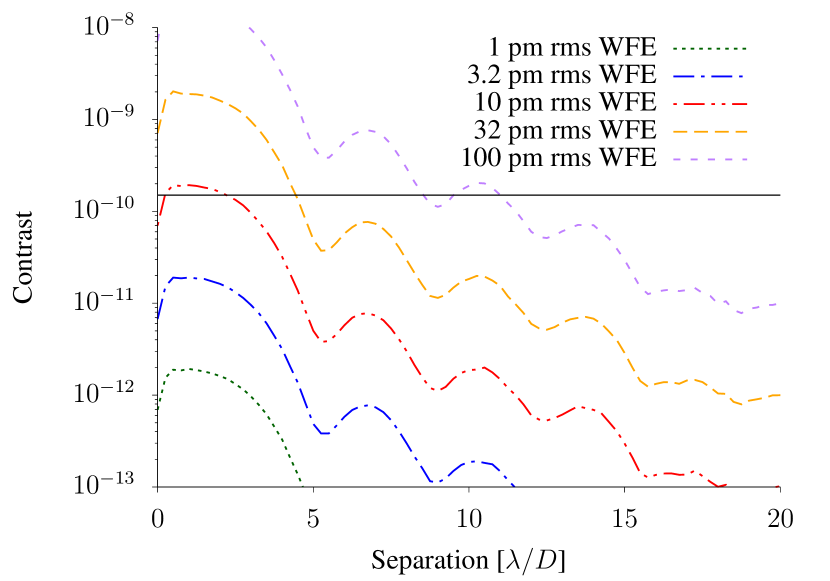
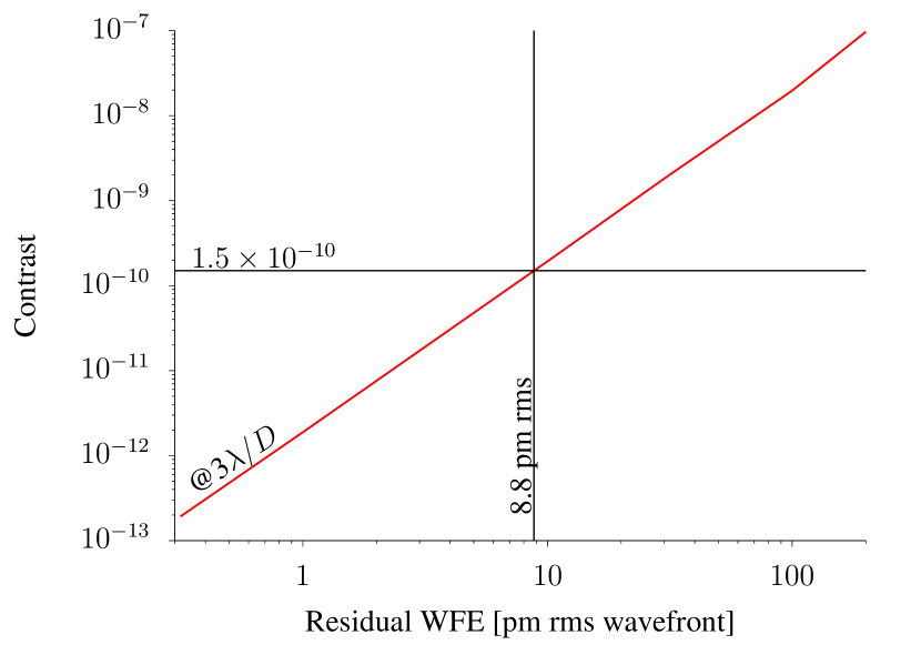
Figure 1: Left: Numerical simulation of contrast versus RMS segment motion wavefront error for an ideal coronagraph. Curves show decreasing wavefront error from top to bottom. A horizontal line indicates the contrast of an Earth-radius exoplanet with an albedo of 0.25 at quadrature. Right: Raw contrast versus residual WFE at 3 $\lambda/D$, showing that 10 pm is a good approximation for a WFE requirement for detection of Earth-like planets with a segmented-aperture telescope.

2.2 Wavefront Error Simulation

This section will explore the relationship between mechanical stability and incident photon rate by applying a control law to the PSD defining segment motion. This will lay the groundwork for setting design constraints on artificial laser guide stars. A realized optomechanical system will have time-dependent OPDs arising from a variety of mechanical disturbances (c.f. Bronowicki (2006); Shi et al. (2016)). To constrain the problem, we assume a smooth PSD. The form of the functional PSD we have chosen for modeling the longer timescale motion of primary mirror segments is similar to previous work, but with a few key differences. Previous work by Lyon & Clampin (2012) assumed a OPD PSD with respect to frequency, $f$, of the form:

$$\mathcal{T}(f)\propto\frac{1}{1+\left(\frac{f}{f_{n}}\right)^{\alpha}}.$$ (1)

Here $\alpha$ is a power law constant and $f_{n}$ is the “knee frequency” where the distribution rolls off. A form commonly used to model optical surfaces (Church & Takacs, 1986, 1991; Toebben et al., 1996; Harvey et al., 2009) is the K-correlation model, which in optical turbulence modeling is known as the von Karmàn PSD (Hardy, 1998; Andrews & Philips, 2005). We adopt the following form as the PSD of the optical path difference due to segment motion:

$$\mathcal{T}_{OPD}(f)=\frac{\beta_{OPD}^{2}}{\left(f_{o}^{2}+f^{2}\right)^{\alpha/2}}$$ (2)

Here $\beta_{OPD}$ is a normalization constant and $f_{o}$ is the knee frequency, which is defined in terms of an “outer time” $T_{0}$ by $f_{0}=1/T_{0}$ (in analogy with the outer scale in turbulence). This has a slightly different form from that used by Lyon & Clampin (2012) for both spatial and temporal PSDs. Fig. 2 directly compares the two similar forms. $f_{0}$ is essentially equivalent to their “drift frequency” $f_{n}$. In addition to its more general use in the literature, we prefer the PSD in Equation 2 to that Equation 1 due to its simpler behavior as $f_{0}\rightarrow 0$, where it trivially becomes pure $1/f^{\alpha}$ noise.

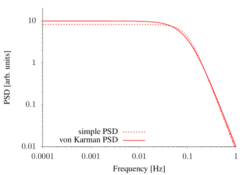
Figure 2: Comparison with arbitrary units of the simple PSD form of Equation 1 with the more general von Karmàn or K-correlation form of Equation 2. For equal knee frequencies, $f_{n}=$0.1 Hz in this case, the forms are very similar. We adopt the von Karmàn PSD in this work.

Whether or not such PSDs are integrable depends on $f_{0}$ and $\alpha$. In order to allow any value of these parameters, we adopt a band-limited stability specification. We call this $\sigma_{10}$, or the “RMS in 10 min”, i.e. “10 pm RMS in 600 sec”. We normalize the PSD accordingly, from the frequency corresponding to 10 minutes to one half of $f_{s}$, the sampling frequency of the wavefront control system, i.e.

$$\beta_{OPD}^{2}=\frac{\sigma_{10}^{2}}{\displaystyle\int_{\frac{1}{600\textrm{ sec}}}^{f_{s}/2}\left(f_{o}^{2}+f^{2}\right)^{-\alpha/2}df}.$$ (3)

The PSD of measurement noise is given by Males & Guyon (2018) as:

$$\mathcal{T}_{p}(f)=\frac{\beta_{p}^{2}}{F_{\gamma}\tau_{wfs}+n_{pix}\sigma_{ron}^{2}}\left(\frac{\tau_{wfs}}{2}\right),$$ (4)

where we are ignoring background noise sources which will not significantly impact the shape of the PSD. $n_{pix}$ is the number of detector pixels used, each with readout noise $\sigma_{ron}$. See Table 1 for assumed noise values and the number of pixels per segment. the measurement noise does not depend on wavefront sensor exposure time, $\tau_{wfs}$, given a noiseless (or low-noise) detector.

To understand the impact of wavefront sensing we select a Zernike wavefront sensor (ZWFS), which has ideal photon noise limited sensitivity across spatial frequencies (Guyon, 2005) and is proposed for the baseline LUVOIR and the Habitable Exoplanet Observatory Mission Concept (HabEx) coronagraph designs (Pueyo et al., 2017; Gaudi et al., 2018). A ZWFS been studied for co-phasing large segmented-aperture space telescopes to the nanometer level (Janin-Potiron et al., 2017), and one is planned for low-order wavefront sensing in the Wide-Field InfrarRed Survey Telescope (WFIRST) coronagraph instrument (Shi et al., 2016). Alternatively, a pyramid wavefront sensor could provide autocalibration of intensity variation, at the expense of increased noise levels (Guyon, 2005). The parameter $\beta_{p}$ describes the sensitivity of the WFS to photon noise for the spatial frequency considered (Guyon, 2005, Appendix A). For a ZWFS measuring rigid-body motion using photons striking a particular segment (Guyon, 2005; N’Diaye et al., 2013),

$$\beta_{p}=\frac{1}{2}.$$ (5)

In Fig. 3 we compare OPD PSD s with a range of $\alpha$ and $T_{0}$ values. This demonstrates 0.01 Hz is the approximate sensing limit due to stellar photon noise per segment, even for bright stars (the stellar magnitude limiting photon noise is shown as horizontal solid lines). For this discussion, natural guide star wavefront sensing is limited to the photons solely within V-band (Bessell, 2005) with the zero-magnitude flux listed in Table 1.

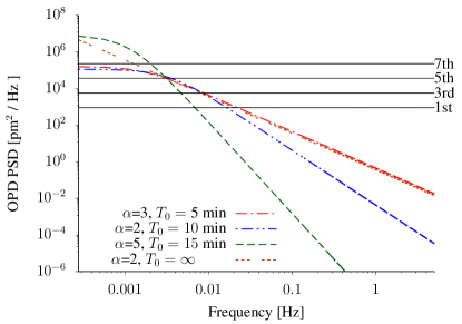
Figure 3: Comparison of PSDs with with different power law constants ($\alpha$) and different $T_{0}$ outer times. The dashed lines show the optical path difference PSDs and the horizontal solid lines show the measurement noise floor for stars of different magnitudes. For $m_{\textrm{V}}$=7 and dimmer stars measurement noise dominates. Even for a steep $\alpha$=5 PSD, stellar noise will dominate above 0.01 Hz for an $m_{\textrm{V}}$=1 star. This sets the $>100$ second stability requirement for natural guide stars. All OPD PSDs are normalized with $\sigma_{10}$ = 10 pm rms.

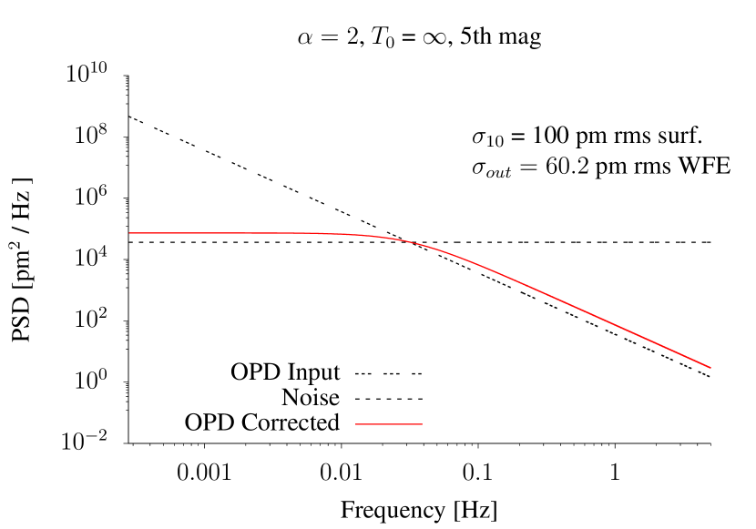
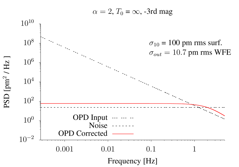
Figure 4: Example application of closed loop control to OPD using $m_{\textrm{V}}$=5 (left) and $m_{\textrm{V}}$=-3 (right) guide stars. The input disturbance is shown as a triple dashed line and the corrected output is a solid line. The photon limited noise floor is shown as a horizontal dashed line.

2.3 Closed Loop Wavefront Control

In order to assess how close the segment position can be controlled to the stellar sensing limits, we apply the framework developed in Males & Guyon (2018) for modeling the dynamics of a closed-loop control system. Given the two PSDs just described, $\mathcal{T}_{OPD}(f)$ (Equation 2) and $\mathcal{T}_{p}(f)$ (Equation 4), the output PSD from a closed-loop control system is given by:

$$\mathcal{T}(f)=\mathcal{T}_{OPD}(f)|ETF(f)|^{2}+\mathcal{T}_{P}(f)|NTF(f)|^{2},$$ (6)

where $ETF(f)$ is the system Error Transfer Function and $NTF(f)$ is the system Noise Transfer Function. These transfer functions describe the action of the control system on the input PSDs, and include the effects of finite integration time, a delay for calculation and communication, and the feedback control law. As expected from Equation 4, the OPD contribution of measurement noise is flat versus frequency, while the power law constant ($\alpha$) drives the slope of the OPD and $T_{0}$ sets the roll off frequency. For the example cases where $\alpha=2$ and $T_{0}=10$ min and $\alpha=3$ and $T_{0}=5$, the OPD floor just barely exceeds the noise floor for a 7th magnitude star, so wavefront control on stars dimmer than 7th magnitude would not benefit such a system.

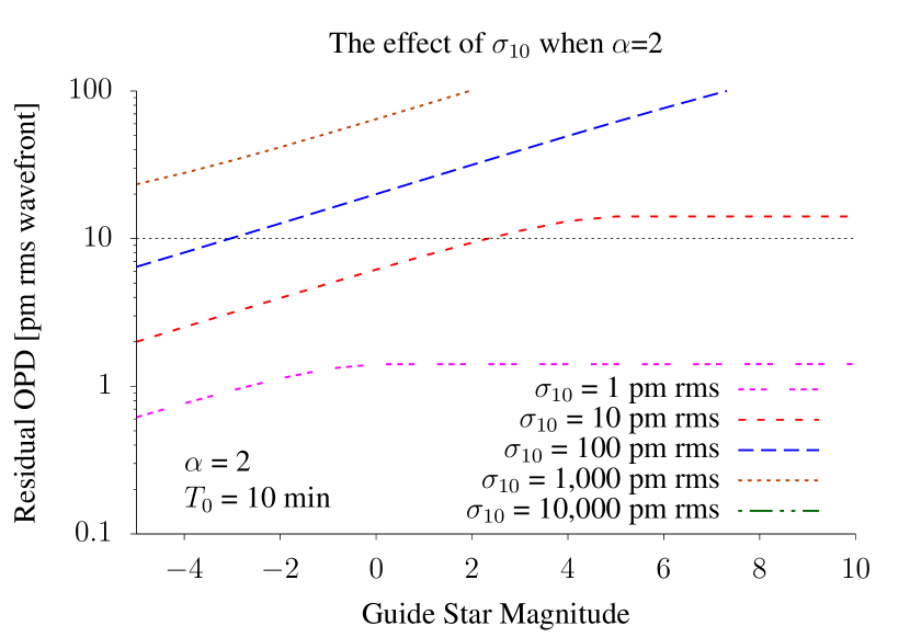
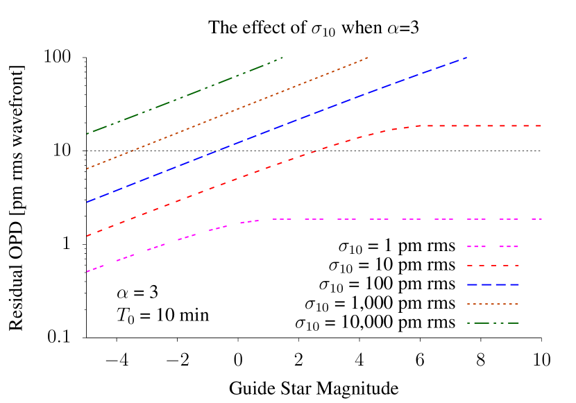
Figure 5: Residual segment disturbance OPD as a function of guide star magnitude for $\alpha=2$ (left) and $\alpha=3$ (right) for $T_{0}=\infty$. The RMS residual across all temporal frequencies, $\sigma_{out}$, for the $m_{\textrm{V}}$=5 star is 60.2 pm which is too high to detect Earth-like exoplanets. Conversely, a hypothetical $m_{\textrm{V}}$=-3 guide star is sufficient to control OPD to 10.7 pm and reach contrasts of $\sim 10^{-10}$.

3 Artificial Laser Guide Star Spacecraft Concept

Rather than guiding on a science star as assumed previously, one might use an artificial guide star to achieve an increased wavefront sensing flux. In order to maintain 10 pm stability while observing dimmer stars, we explore the potential of a formation-flying spacecraft with a continuous-wave light source, providing more photons than a natural star. The geometry of the LGS concept is shown in Fig. 6. The segmented space telescope with radius $R_{T}$ is shown at left. The LGS is shown at a distance $z$, projecting a Gaussian laser beam (to ensure smooth propagation) with a divergence, $\theta$, at the telescope. While the telescope observes a target star at some astronomical coordinate, the LGS appears offset by some angle $d\alpha$. Table 1 includes several key parameters of the system we will consider for the design trades throughout this work. Section 4 will describe the design constraints on an LGS for augmenting an Earth-like exoplanet coronagraph mission using typical telescope properties drawn from recent publications covering the design of the LUVOIR mission concept (Pueyo et al., 2017; Feinberg et al., 2017).

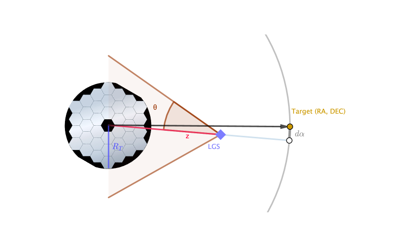
Figure 6: Two dimensional representation of the LGS observing scenario. The observing telescope (left) direction of regard is shown as a vector projected onto the celestial sphere (right), while at range $z$ the LGS (tilted square) is offset from the direction of regard by angle $d\alpha$. The width of the Gaussian LGS beam, with a half-width divergence $\theta$, is shaded.

Table 1: System parameters assumed in wavefront sensing and control calculations.

Parameter	Value	Notes
Telescope Diameter	9.2 m	Feinberg et al. (2017)
Segment Geometry	Hexagonal	Eisenhower et al. (2015)
Segment face-to-face width	1.15 m	LUVOIR A (Pueyo et al., 2017)
Zero-mag photon flux	9.1$\times 10^{9}$ photons/sec	Vega-based, in Bessel V band
System Throughput, $T_{p}$	0.1	including detector QE
$\lambda$	500 nm
Loop update rate	10 Hz
Loop delay	1.5 msec
$\Delta f$	1/3600	The PSDs model 1 hour periods
$n_{pix}$	16/segment
$\sigma_{ron}$	0.3 $e^{-}$/pixel/frame	typical EMCCD read noise

4 Results

4.1 Photon and Sensor Noise

The photon noise rate per segment places a limit on the sensing of the segment position. The closed-loop analysis of Section 2.3 relates guide star magnitude, natural or artificial, to residual wavefront error. Fig. 4 shows the input OPD is well-corrected to near the noise floor at low frequencies. The input disturbance is shown as a triple-dashed line and is suppressed in the controlled curve (solid line) by more than six orders of magnitude at low frequencies. Wavefront control could be implemented through direct control of segments via a hexapod (e.g. Contos et al. (2006)), or a deformable mirror (two high-actuator count microelectromechanical systems (MEMS) deformable mirrors are planned for LUVOIR (Pueyo et al., 2017)). The most important parameter is the overall level of vibrations, which we have characterized as the 10 minute RMS, $\sigma_{10}$. The challenge of controlling these vibrations is shown in Fig. 5 for the case of $\sigma_{10}$ = 10 min and $\alpha$ = 2 (left panel) and $\alpha=3$ (right panel). For $\sigma_{10}$ = 10 pm, a 10 pm residual OPD is achieved for an 2nd magnitude or brighter guide star star. This would limit coronagraphy of a Sun-like stars to within just 3 parsecs for natural guide stars and sets a useful lower limit on the dimmest LGS for Earth-like exoplanet imaging. To control much larger disturbances, such as $\sigma_{10}$ = 1 nm residual OPD, a $m_{\textrm{V}}$ = -2 or brighter guide star is needed.

4.2 Pointing Sensitivity

In addition to variations in the pupil plane intensity due to photon noise, changes in the guide star illumination pattern must also be considered in order to set the LGS performance requirements. Unlike the even illumination pattern of a natural guide star, the LGS beam will have a Gaussian intensity distribution. As discussed Section 4.1, the ZWFS is sensitive to both intensity and phase variations. The ZWFS is effectively an interferometric fringe pattern at a single relative phase shift. Thus, intensity variations lead to spurious phase measurements. This is a concern for the LGS because the Gaussian laser beam will produce a variable illumination pattern across the observatory pupil, which moves according to the pointing of the LGS relative to the observatory ($d\alpha$ in Fig. 6).

In addition to photon noise, if the pupil intensity function is changing on the time scale of segment jitter, due to changes in the pointing of the LGS, the WFS will sense erroneous tilts across the pupil. If the Gaussian function is static across the pupil, then it is straightforward to calibrate a static non-uniform intensity function. For example, Fig. 7 shows a simple numerical model of a ZWFS generated using the Fresnel propagation environment in the Physical Optics Propagation in PYthon library Perrin et al. (2016). A Gaussian intensity distribution (left panel), and a flat phase (middle panel) define the input wavefront. For simplicity and to maintain the optimal choice of mask diameter, the hexagonal aperture was truncated to a circumscribed circle for this simulation. After propagation to the image plane and multiplication by a complex phase mask with the optimal diameter (N’Diaye et al., 2013) of 1.06$\lambda$ and $\theta=\pi/2$, propagation to the next pupil plane gives the measured pupil intensity shown in the right hand panel of Fig. 7. For small phase shifts $\phi$, and an intensity $I$ in a ZWFS pixel, (N’Diaye et al., 2013, Equation 15) gives the linear relation between phase and intensity as:

$$\phi=I/I_{0}-0.5.$$ (7)

$I_{0}$ is the average intensity across the pupil. Differentiating shows the phase measurement error as a function of intensity error $dI$ is:

$$d\phi=dI/I_{0}.$$ (8)

We quantify the pointing jitter error by calculating the fractional intensity difference between an on-axis LGS Gaussian beam striking the telescope $I_{1}^{\prime}$, and $I_{2}^{\prime}$, the same beam offset by $x_{0}$:

$$dI/I=\frac{I_{1}^{\prime}-I_{2}^{\prime}}{I_{0}}=e^{\frac{-2x^{2}}{w^{2}}}-e^{\frac{-2(x+x_{0})^{2}}{w^{2}}}$$ (9)

Where $x$ is the radial displacement from gaussian beam, $w$ is the beamwidth, and $I_{0}$ is the intensity. For x=0, then $dI/I^{\prime}=1-e^{\frac{-2x_{0}^{2}}{w^{2}}}$. The first order Taylor expansion is:

$$d\phi\approx dI=1-\left(1-\frac{2x_{0}^{2}}{w^{2}}\right)=\frac{2x_{0}^{2}}{w^{2}}.$$ (10)

Plugging in a minimum required phase error of 10 pm and a pointing error between measurements (e.g. 15 mas) lets us solve for the minimum beamwidth $w$. Due to the need to stabilize intensity across the pupil, this gives in a ratio of divergence versus transmitter jitter of $>380$, which is much larger the typical values used to maximize received intensity for similar applications such as laser communications (e.g. ratio of divergence versus transmitter jitter of $\sim 10$, Clements et al. (2016)). For LGS jitter of 15 mas, a level of performance regularly exceeded 3$\times$ by previous space observatories (e.g. Nurre et al. (1995); Koch et al. (2010); Mendillo et al. (2012)), the divergence required to keep the jitter induced errors within 10 pm is $>0.325^{\prime\prime}$, limited by the mode-field diameter ($MFD$) and allows more feasible laser powers.

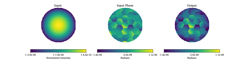
Figure 7: Example of ZWFS with a LGS, illustrating that a Gaussian input beam and a flat input phase disturbed by random segment motion (middle) leads to an varying output intensity (right) which is degenerate with phase errors. Accurate LGS pointing allows for quasi-static measurement of the intensity distribution and correction of this error. This simulation used $w=23.40^{\prime\prime}$ at a range of 4.4 $\times 10^{4}$ km, which corresponds to a beam-width of 4.7 km at the telescope.

4.2.1 Beam Divergence Limitations

The finite size of a single-mode fiber generating the LGS beam and diffraction from the exit aperture further limit the minimum LGS beam divergence. The fiber mode-field diameter half-angle divergence is given by:

$$\theta_{MFD}=MFD/(2f)$$ (11)

where $MFD$ is the mode field diameter of the optical fiber and $f$ is the focal length of the collimating optics. In addition to the mode-field diameter, the size of the exit aperture constrains the beam divergence. Likewise, for a Gaussian beam, the half-angle beam divergence is given by:

$$\theta_{w}=\lambda/(\pi w_{0}).$$ (12)

where $w_{0}$ is the beam waist (Kogelnik & Li, 1966, Equation 22). To minimize diffraction effects, we assume $w_{0}$ is one third or less of the LGS exit aperture radius.

4.3 Wavelength Selection

The LGS may contribute background signal to science observations via scattered light, thermal emission, and fluorescence. A longer-than-science wavelength out-of-band laser source minimizes fluorescence and scattering internal to the telescope (e.g. via dichroic filters) while a high-efficiency laser minimizes waste heat. For simplicity, in this initial study, we will consider two common laser wavelengths, 980 nm and 532 nm. Longer wavelengths allow a decrease in the range between the LGS and telescope (Section 4.4), and a 980 nm source is within the sensitivity range of silicon detectors. Efficiency is also critical to designing a spacecraft with feasible thermal control, and 980 nm lasers have been previously shown to have provide better than $50\%$ wall-plug efficiency in continuous operation (Crump et al., 2005). Alternatively, the guide laser could be blocked by a narrow line-blocking interferometric filter. As described in Section 4.4, a shorter wavelength could provide a reference source closer to the center of the visible light science band Pueyo et al. (2017).

4.4 LGS Formation Flying Range

Since the LGS is a finite distance from the telescope, we must account for the defocus of the reference wavefront. For a spherical wave emanating from the LGS at distance $z$ (the range to the center of the entrance aperture), the Peak-to-Valley (PV) defocus is given by difference between $z$ and $R_{C}$, the range to the edge of the aperture. Solving for $R_{C}$ as a function of telescope aperture and the peak-to-valley wavefront error across the pupil $PV_{WFE}$:

$$R_{C}=\frac{PV_{WFE}^{2}+R_{T}^{2}}{2PV_{WFE}}\approx\frac{R_{T}^{2}}{2PV_{WFE}},$$ (13)

for a telescope radius $R_{T}$. . Hence, for PV wavefront error less than $\pi/2$,

$$R_{C}=2R_{T}^{2}/\lambda.$$ (14)

Thus, the minimum range to the baseline telescope is 43,184 km at 980 nm. The addition of a defocusing mechanism in front of the wavefront sensor would relax this requirement, but may add non-common path errors and tighten the lateral stability requirement discussed in Section 4.5.

4.5 LGS position

This section will quantify the station keeping needed, or the accuracy with which the LGS must be held on the telescope-target-star vector during a coronagraphic exposure. Motion of the LGS across the sky relative to the target star will appear as a tilt to a telescope WFS. For the purpose of this study, we presume the telescope pointing is highly stabilized onboard, such as by a Fine Guidance Sensor (FGS) (Nurre et al., 1995), and that any bulk tilts across the wavefront sensor will be subtracted. In order to enable effective tracking of the LGS, one might require it to hold position to within 0.25$\lambda/D$ from the target star ($d\alpha$ in Fig. 6). At the baseline range, this corresponds to a cross-track stability of 1 meter, comparable to the requirements of starshade missions (e.g. Soto et al. (2017)).

would also keep the LGS keeps the wavefront tilt within the range of the ZWFS without an additional tip-tilt mirror in the wavefront sensing path, minimizing sensing of spurious off-axis aberrations.

Reflected sunlight from the LGS could contribute incoherent background to coronagraphic observations. For example, neglecting the solar panel reflectivity, given a 300 mm $\times$ 300 mm spacecraft cross section, at $5\times 10^{4}$ km range with an an albedo of 0.01, the scattered light is $m_{\textrm{V}}=16$. A carbon nanotube coated spacecraft could potentially lower the albedo to 0.001, bringing the scattered light as low as $m_{\textrm{V}}$=19 (Cartwright, 2015). This scattered light further motivates keeping the LGS well within the inner working angle, as sources inside $\lambda/D$ will be attenuated by many orders of magnitude by most coronagraph designs (e.g. N’Diaye et al. (2016); Trauger et al. (2016); Zimmerman et al. (2016))

4.6 Other considerations

The LUVOIR concept includes simultaneous observations in Ultraviolet (UV), visible, and Infrared (IR) with one channel serving as the wavefront sensor (Pueyo et al., 2017). As with reflected sunlight, discussed in Section 4.5, thermal emission of the spacecraft may contribute a significant background if the source is not behind the coronagraph mask.

For LGS wavelengths shorter than the science wavelength, the magnitude of fluorescence from transmissive optics (Engel et al., 2003), and the potential for laser induced contamination of reflecting surfaces (Wagner et al., 2014) will require consideration. Fluorescence effects are dependent on material and wavelength. Thus, testing of materials and wavelength selection, along with consideration of a multi-wavelength LGS transmitter, is expected to mitigate these effects.

5 Discussion

There are two key benefits to the LGS approach: the ability to directly image dimmer target star systems, and decreasing the mechanical stability requirements on the telescope. Designs at opposite extremes of possible LGS transmitted power are shown in Table 2. Equation 14 sets the range for the mission concepts for two laser wavelengths, 532 nm and 980 nm. Both rely on an accurately pointed guide star to provide constant intensity calibration where the pupil intensity function is held constant throughout the observation. For example, a “well controlled” 5 W LGS case uses a bright guide star which can be sampled quickly at hundreds of Hertz while a "stable" case assumes a relatively stable telescope (e.g. $\sigma_{10}=10$ pm) requiring fewer photons per second for WFS ing, is shown to compare science performance with and without the LGS. The magnitude values in $V$ band are directly comparable to the x-axis of Fig. 5, allowing estimation of the residual OPD given a known input OPD PSD. For example, Case VI allows correction of a 1000 pm RMS input OPD to 10 pm RMS for $\alpha=3$. $z^{\prime}$ magnitudes are given for the 980 nm LGS cases.

Table 2: LGS transmitter design parameters possible scenarios where an LGS illuminates a segmented telescope. The “stable” telescope cases, Cases II and IV, are based on recent designs for a well-damped telescope using natural guide stars for wavefront sensing. The controlled cases, Cases I, III, V, and VI, would use a more powerful laser to enable faster update, relaxing telescope stability requirements. Throughput here refers to total observatory sensitivity, including the impacts of coating reflectivity and detector quantum efficiency. Transmitter jitter here is the maximum allowable excursion of the LGS beam from the bore-sight of the telescope. The rightmost “band” column indicates the filter over which the effective magnitude, $m$, is calculated.

Case	Telescope	Laser Power	$\lambda_{WFS}$	$z$	Throughput	$\theta$	Transmitter jitter	$m$	band
		$\mathrm{W}$	$\mathrm{nm}$	$\mathrm{km}$		$\arcsec$	$\arcsec$
I	Controlled	5.0	980.0	43184.0	0.1	3.861	0.015	-7.1	z’
II	Stable Telescope	0.005	980.0	43184.0	0.1	3.861	0.015	0.4	z’
III	Controlled	5.0	532.0	79549.0	0.1	3.861	0.015	-4.9	V
IV	Stable Telescope	0.005	532.0	79549.0	0.1	3.861	0.015	2.6	V
V	Controlled	5.0	980.0	43184.0	0.1	12.49	0.1	-4.5	z’
VI	Controlled	5.0	532.0	79549.0	0.1	12.49	0.1	-2.3	V

5.1 Controlled Case: Relaxed Telescope Stability

In addition to increasing the available discovery space, an LGS has the potential to drastically relax telescope stability requirements. Since the system control authority is no longer limited by photon noise, primary mirror segments can be actively held in position. For example, Fig. 5 shows that, for $\alpha=3$, a $m_{\textrm{V}}$ = -4 or dimmer guide star (cases I, III, and V in Table 2) could provide 10 pm segment control for a $\sigma_{10}$ = 1 nm input disturbance when $T_{0}=$ 10 min. This is a more than two orders of magnitude of relaxation in telescope stability compared to performing wavefront sensing using photons from a $m_{\textrm{V}}$ = 5 science target. Alternatively, a shorter $T_{0}$ could be controlled with a brighter LGS or a smaller $\sigma_{10}$.

5.2 Stable Case: Increased Discovery Space

It is illustrative to estimate how reducing wavefront sensing noise impacts science yield for a telescope built with sufficient segment stability to reach $10^{-10}$ contrasts around $m_{\textrm{V}}$ = 5 stars.

A highly corrected telescope coupled with an LGS would open up a large population of nearby candidate host stars to greater than $10^{-10}$ contrast imaging with future space telescopes with a low-power $\lesssim$50 mW LGS transmitter. This scenario for 532 nm and 980 nm laser wavelengths is shown in cases II and IV in Table 2. These stars may not be ideal for uninformed searches due to the longer exposure times required, but if more rocky exoplanets are discovered by upcoming sub-1 m/s radial velocity surveys of stars as dim as V=12 (e.g. Halverson et al. (2016)), the capacity for high-contrast imaging of stars with low apparent magnitude will be valuable.

For a well stabilized telescope, the transmitter jitter requirement for the LGS could be relaxed from the 15 mas discussed in Section 4.2. Given the divergence and pointing constraints discussed in Section 4.2, Case V and VI show that example systems with a relaxed transmitter jitter of 0.1^′′ and correspondingly increased $\theta$ still result in a guide star that is several magnitudes brighter than science targets, providing several magnitudes of margin on 10 pm segment rigid-body sensing.

Figure 8: Rendering of a 30 cm $\times$ 30 cm $\times$ 30 cm (27U) small satellite guide star built around a spherical fuel tank. A notional laser transmitter is shown in the upper left. Low reflectivity paneling and photovoltaic panels are not shown.

Previous research has suggested that 10 minute stability at the 10 picometer level is necessary for the detection of Earth-like planets around 5th to 6th magnitude stars (Stahl et al., 2013, 2015). The analysis presented here shows that the combination of a limiting magnitude of $m_{\textrm{V}}$ = 5 to $m_{\textrm{V}}$ = 6 and $\sigma_{10}$ = 10 minutes may be overly optimistic. The ideal coronagraph model output shown in Fig. 1 supports the previous finding that 10 pm control of segment motion is necessary to reach contrasts of $10^{-10}$ at the IWA. However, after accounting for system transmission, detector noise, and photon noise using a closed-loop control law, Fig. 5 shows controlling segment rigid-body motion to this level requires guide star magnitudes $m_{\textrm{V}}$ < $3$.

Unfortunately, many promising, nearby, exoplanet host stars are dimmer than either 3rd or 5th magnitude, particularly M-dwarf stars, which may host the majority of terrestrial planets (Dressing & Charbonneau, 2015; Shields et al., 2016). While the habitable zone is still largely unconstrained (see discussion in Seager (2013)); we explore the flux ratio of a canonical Earth-radius planet ($R_{\oplus}$) at the Earth equivalent insolation distance, $r_{eei}$. This flux ratio is given by

$$\zeta_{\oplus}=\frac{A\Theta(\alpha)R^{2}_{\oplus}}{r^{2}_{eei}}.$$ (15)

Fig. 9 plots $m_{\textrm{V}}$ versus $\zeta_{\oplus}$ using data from ExoCat-1 (Turnbull, 2015), for planets at the Earth-equivalent insolation distance with geometric albedo $A=0.2$ and a typical $\Theta=1/\pi$ phase function value (Robinson et al., 2015). These targets can be broken into four quadrants around the canonical Earth-Sun value at 10 pc, indicated with an encircled cross just above $10^{-10}$ at slightly below $m_{\textrm{V}}=5$. Below 10^-10 are hotter stars with habitable zones at farther separations. Dimmer than 5th magnitude, the majority of target stars are cooler than the Sun with slightly larger $\zeta_{\oplus}$ values, but there is a significant population of Sunlike and hotter stars within 30 parsecs with lower $\zeta_{\oplus}$ values which will be particularly hard to access with natural guide star sensing. The right panel of Fig. 9 shows the cumulative distribution versus $m_{\textrm{V}}$ for the Research Consortium On Nearby Stars (RECONS) nearest 100 stars, and the EXOCAT-1 catalog of promising exoplanet host stars (Turnbull, 2015). There are 463 exoplanet candidate host stars with $m_{\textrm{V}}\leq$ 5 within 30 pc in the ExoCat-1 catalog and more than four times as many stars if the limiting magnitude is instead extended to 10th magnitude. As can be seen from the shading of points in Fig. 9, many of these dim stars are cooler than the Sun, with less stringent contrast requirements. There are hundreds more stars between 5th and 8th magnitude with comparable flux ratios to the Earth at 1 AU from the Sun. For the more conservative $m_{\textrm{V}}<3$ limit found here, there are only 142 target stars visible. An LGS allows recovery of the contrast needed to search the future mission target stars for Earth-like planets with a coronagraph. Alternatively, a telescope stability, $\sigma_{10}$, $<10$ pm or a stability outer time, $T_{O}$, $>$10 minutes is needed.

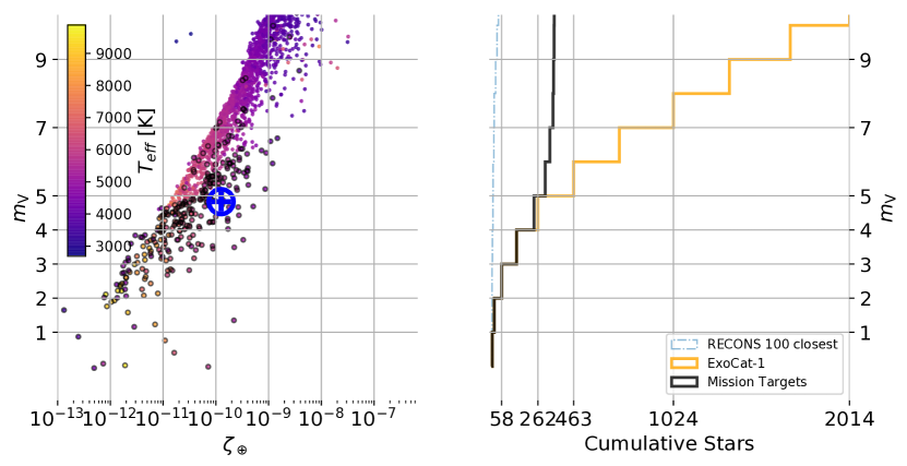
Figure 9: Left: Magnitude vs flux ratio of a 1$R_{\oplus}$ planet at the Earth-equivalent insolation distance for stars in the ExoCat database below 10,000 Kelvin (Turnbull, 2015). The sun at 10 parsecs is shown as the encircled cross. Black outlined stars have been previously flagged by NASA missions as priorities for the WFIRST (Kasdin et al., 2018), LBTI (Ertel et al., 2018), Exo-S (Seager et al., 2015), and Exo-C (Stapelfeldt et al., 2015) projects in the Exoplanet Archive. Right: The cumulative number of target stars as function of magnitude. There are 40 stars brighter than 10th magnitude in the RECONS databases of the closest stars and 2,014 in ExoCat. Natural guide star wavefront sensing and 10 minute telescope stability place a limit at 3th magnitude or brighter which leaves 142 ExoCat stars accessible. The solid black line shows the same mission stars as are circled in the left panel.

6 Summary

This paper is intended to serve as a starting point in the explorations of design space for a LGS to control segmented telescope motion. We have summarized the key design parameters, including inter-spacecraft range, source wavelength, station keeping, and laser transmitter jitter for a spacecraft formation flying along the direction of regard of a segmented-aperture coronagraphic space telescope to provide a bright reference wavefront. By applying a closed-loop transfer function to wavefront control of rigid-body motion for the nominal LUVOIR segment geometry, we derive a wavefront sensing limiting magnitude for detection of Earth-like planets of $m_{\textrm{V}}<3$ with an ideal coronagraph, given 10 minute telescope stability. The LGS concept as described enables relaxation of telescope segment stability by up to two orders of magnitude and offers the potential for nearly an order of magnitude increase in the number stars observable to $10^{-10}$ raw contrast without wavefront sensing limitations.

This work will be followed by more detailed studies to optimize LGS feasibility and performance. Areas where further design studies are required include the number and lifetime of LGS spacecraft, range compensating wavefront sensor fore-optics, and alternative wavefront sensor architectures. In particular, laser wavelengths could be significantly shorter or longer; either increasing the sensitivity per photon or decreasing the wavefront curvature at a given range. Decreasing curvature would allow the LGS to fly closer and decrease maneuvering costs. It may be possible to trade these notional requirements for increased system complexity. For example, a focus and pointing correction stage could allow shorter LGS-telescope separations and relaxed station keeping requirements. Studies and laboratory simulations of the non-common-path ray propagation and higher-order diffraction effects of such solutions are presently underway (Xin et al.  in preparation, and (Lumbres et al., 2018).

Large disturbances with steep power law distributions, $\alpha>3$, are readily correctable by a LGS of feasible brightness, which potentially enables relaxed segment positional stability requirements, decreasing the engineering changes relative to the structural design of the James Webb Space Telescope (JWST). Predictive control (Males & Guyon, 2018) could also improve performance at resonance frequencies. For example, JWST has a 20 nm RMS segment “rocking” mode at $\sim$40 Hz (Stahl et al., 2015). The results above show care must be taken to specify the full PSD envelope of OPD disturbances, otherwise the actual limiting magnitude may be much brighter than expected.

The details of the LGS transmitter needed to provide precision pointing, particularly whether it is stabilized by a fine pointing system or body pointing, are the subject of future work along with development of control laws and quantification of the noise requirements for the attitude sensors and actuators.

Efforts are underway (captured in Clark et al., in preparation) to also develop mission architectures and spacecraft designs that optimize in terms of terrestrial planet yield while integrating state-of-the art power, thermal, and propulsion technologies. . Coordination between multiple LGS in order to minimize delay between observations could significantly increase observing efficiency; a similar approach has been proposed for starshades, which have more complex systems with stringent requirements on fabrication, deployment, attitude, and navigation (Stark et al., 2016a).

References

- Allan et al. (2018) Allan, G., Douglas, E. S., Barnes, D., et al. 2018, in Proc SPIE, Vol. 10698, 1069857
- Andrews & Philips (2005) Andrews, L. C., & Philips, R. L. 2005, Laser Beam Propagation through Random Media, 2nd edn. (SPIE)
- Basden et al. (2018) Basden, A., Brown, A. M., Chadwick, P., Clark, P., & Massey, R. 2018, Monthly Notices of the Royal Astronomical Society, 477, 2209
- Beckers et al. (1982) Beckers, J. M., Poland, C., Ulich, B. L., et al. 1982, in Advanced Technology Optical Telescopes I, Vol. 0332 (International Society for Optics and Photonics), 42
- Bessell (2005) Bessell, M. S. 2005, Annual Review of Astronomy and Astrophysics, 43, 293
- Bolcar (2017) Bolcar, M. R. 2017, in Proc SPIE, Vol. 10398 (International Society for Optics and Photonics), 103980A
- Bolcar (2018) Bolcar, M. R. 2018, LUVOIR Optical Train Throughput?
- Bouchez et al. (2012) Bouchez, A. H., McLeod, B. A., Acton, D. S., et al. 2012, in Adaptive Optics Systems III, Vol. 8447 (International Society for Optics and Photonics), 84473S
- Bronowicki (2006) Bronowicki, A. J. 2006, Journal of Spacecraft and Rockets, 43, 45
- Cartwright (2015) Cartwright, J. 2015, Phys. World, 28, 25
- Church & Takacs (1986) Church, E. L., & Takacs, P. Z. 1986, in , 107
- Church & Takacs (1991) Church, E. L., & Takacs, P. Z. 1991, in Proc. SPIE, Vol. 1530, Optical Scatter: Applications, Measurement, and Theory, ed. J. C. Stover, 71
- Clements et al. (2016) Clements, E., Aniceto, R., Barnes, D., et al. 2016, SPIE
- Contos et al. (2006) Contos, A. R., Acton, D. S., Atcheson, P. D., et al. 2006, in Pr, ed. J. C. Mather, H. A. MacEwen, & M. W. M. de Graauw, 62650X
- Crump et al. (2005) Crump, P., Wang, J., Crump, T., et al. 2005, Optimized Performance GaAs-Based Diode Lasers: Reliable 800-Nm 125W Bars and 83.5% Efficient 975-Nm Single Emitters, Tech. rep., NLIGHT PHOTONICS CORP VANCOUVER WA
- Douglas (2018) Douglas, E. 2018, Zenodo
- Dressing & Charbonneau (2015) Dressing, C. D., & Charbonneau, D. 2015, The Astrophysical Journal, 807, 45
- Eisenhower et al. (2015) Eisenhower, M. J., Cohen, L. M., Feinberg, L. D., et al. 2015, in Proc SPIE, Vol. 9602 (International Society for Optics and Photonics), 96020A
- Engel et al. (2003) Engel, A., Becker, H.-J., Sohr, O., Haspel, R., & Rupertus, V. 2003, in Advanced Characterization Techniques for Optics, Semiconductors, and Nanotechnologies, Vol. 5188 (International Society for Optics and Photonics), 182
- Ertel et al. (2018) Ertel, S., Defrère, D., Hinz, P., et al. 2018, arXiv:1803.11265 [astro-ph], arXiv:1803.11265 [astro-ph]
- Feinberg et al. (2017) Feinberg, L., Bolcar, M., Knight, S., & Redding, D. C. 2017, in Proc SPIE, Vol. 10398 (International Society for Optics and Photonics), 103980E
- Foy & Labeyrie (1985) Foy, R., & Labeyrie, A. 1985, Astronomy and Astrophysics, 152, L29
- Gaudi et al. (2018) Gaudi, B. S., Seager, S., Mennesson, B., et al. 2018, ArXiv e-prints, 1809, arXiv:1809.09674
- Ginsburg et al. (2018) Ginsburg, A., Sipocz, B., Parikh, M., et al. 2018, Astropy/Astroquery: V0.3.8 Release, Zenodo
- Gonte et al. (2008) Gonte, F., Araujo, C., Bourtembourg, R., et al. 2008, in Ground-Based and Airborne Telescopes II, Vol. 7012 (International Society for Optics and Photonics), 70120Z
- Greenaway & Smith (1990) Greenaway, A. H., & Smith, D. M. 1990, ESA Journal, 14, 169
- Guyon (2005) Guyon, O. 2005, The Astrophysical Journal, 629, 592
- Halverson et al. (2016) Halverson, S., Terrien, R., Mahadevan, S., et al. 2016, arXiv:1607.05634 [astro-ph], 99086P
- Hardy (1998) Hardy, J. W. 1998, Adaptive Optics for Astronomical Telescopes
- Harvey et al. (2009) Harvey, J. E., Choi, N., Krywonos, A., & Marcen, J. G. 2009, in Proc. SPIE, Vol. 7426, Optical Manufacturing and Testing VIII, 74260I
- Henry et al. (2018) Henry, T. J., Jao, W.-C., Winters, J. G., et al. 2018, The Astronomical Journal, 155, 265
- Hicks et al. (2018) Hicks, B. A., Jahoda, K., Petrone, P., Sheets, T., & Boyd, P. 2018, in Space Telescopes and Instrumentation 2018: Optical, Infrared, and Millimeter Wave, Vol. 10698 (International Society for Optics and Photonics), 106986M
- Holzlöhner et al. (2010) Holzlöhner, R., Rochester, S. M., Bonaccini Calia, D., et al. 2010, Astronomy and Astrophysics, 510, A20
- Hunter (2007) Hunter, J. D. 2007, Computing In Science & Engineering, 9, 90
- Janin-Potiron et al. (2017) Janin-Potiron, P., N’Diaye, M., Martinez, P., et al. 2017, Astronomy & Astrophysics, 603, A23
- Jared et al. (1990) Jared, R. C., Arthur, A. A., Andreae, S., et al. 1990, in Proc SPIE, Vol. 1236, 996
- Jones et al. (2001) Jones, E., Oliphant, T., & Peterson, P. 2001, http://www. scipy. org/
- Kasdin et al. (2018) Kasdin, N. J., Turnbull, M., Macintosh, B., et al. 2018, in Space Telescopes and Instrumentation 2018: Optical, Infrared, and Millimeter Wave, Vol. 10698 (International Society for Optics and Photonics), 106982H
- Koch et al. (2010) Koch, D. G., Borucki, W. J., Basri, G., et al. 2010, ApJL, 713, L79
- Kogelnik & Li (1966) Kogelnik, H., & Li, T. 1966, Appl. Opt., AO, 5, 1550
- Landulfo et al. (2018) Landulfo, E., Guardani, R., Macedo, F. M., et al. 2018, in Lidar Technologies, Techniques, and Measurements for Atmospheric Remote Sensing XIV, Vol. 10791 (International Society for Optics and Photonics), 107910B
- Leboulleux et al. (2018) Leboulleux, L., Sauvage, J.-F., Pueyo, L., et al. 2018, arXiv:1807.00870 [astro-ph], arXiv:1807.00870 [astro-ph]
- Lumbres et al. (2018) Lumbres, J., Males, J., Douglas, E., et al. 2018, in Adaptive Optics Systems VI, Vol. 10703 (International Society for Optics and Photonics), 107034Z
- Lyon & Clampin (2012) Lyon, R. G., & Clampin, M. 2012, OE, OPEGAR, 51, 011002
- Lyon & Clampin (2012) Lyon, R. G., & Clampin, M. 2012, Optical Engineering, 51, 011002
- Macintosh et al. (2006) Macintosh, B., Troy, M., Doyon, R., et al. 2006, in Advances in Adaptive Optics II, Vol. 6272 (International Society for Optics and Photonics), 62720N
- Males & Guyon (2018) Males, J. R., & Guyon, O. 2018, JATIS, JATIAG, 4, 019001
- Males & Guyon (2018) Males, J. R., & Guyon, O. 2018, Journal of Astronomical Telescopes, Instruments, and Systems, 4, 019001
- Marlow et al. (2017) Marlow, W. A., Carlton, A. K., Yoon, H., et al. 2017, Journal of Spacecraft and Rockets, 54, 621
- Martinez et al. (2018) Martinez, P., Janin-Potiron, P., Beaulieu, M., et al. 2018, in Adaptive Optics Systems VI, Vol. 10703 (International Society for Optics and Photonics), 1070357
- Max et al. (1997) Max, C. E., Olivier, S. S., Friedman, H. W., et al. 1997, Science, 277, 1649
- Mendillo et al. (2012) Mendillo, C. B., Chakrabarti, S., Cook, T. A., Hicks, B. A., & Lane, B. F. 2012, Appl. Opt., 51, 7069
- Mendillo et al. (2015) Mendillo, C. B., Brown, J., Martel, J., et al. 2015, in Techniques and Instrumentation for Detection of Exoplanets VII, Vol. 9605, 960519
- Mier-Hicks & Lozano (2017) Mier-Hicks, F., & Lozano, P. C. 2017, Journal of Guidance, Control, and Dynamics, 40, 642
- Miller et al. (2015) Miller, K., Guyon, O., Codona, J., Knight, J., & Rodack, A. 2015, in Techniques and Instrumentation for Detection of Exoplanets VII, Vol. 9605 (International Society for Optics and Photonics), 96052A
- N’Diaye et al. (2013) N’Diaye, M., Dohlen, K., Fusco, T., & Paul, B. 2013, Astronomy & Astrophysics, 555, A94
- N’Diaye et al. (2016) N’Diaye, M., Soummer, R., Pueyo, L., et al. 2016, ApJ, 818, 163
- Nurre et al. (1995) Nurre, G. S., Sharkey, J. P., Nelson, J. D., & Bradley, A. J. 1995, Journal of Guidance, Control, and Dynamics, 18, 222
- Pérez & Granger (2007) Pérez, F., & Granger, B. 2007, Computing in Science Engineering, 9, 21
- Perrin et al. (2016) Perrin, M., Long, J., Douglas, E., et al. 2016, Astrophysics Source Code Library, ascl:1602.018
- Perrin et al. (2003) Perrin, M. D., Sivaramakrishnan, A., Makidon, R. B., Oppenheimer, B. R., & Graham, J. R. 2003, ApJ, 596, 702
- Postman et al. (2009) Postman, M., Argabright, V., Arnold, B., et al. 2009, arXiv:0904.0941 [astro-ph], arXiv:0904.0941 [astro-ph]
- Pueyo et al. (2017) Pueyo, L., Zimmerman, N., Bolcar, M., et al. 2017, in Proc SPIE, Vol. 10398 (International Society for Optics and Photonics), 103980F
- Racine et al. (1999) Racine, R., Walker, G. A. H., Nadeau, D., Doyon, R., & Marois, C. 1999, Publications of the Astronomical Society of the Pacific, 111, 587
- Robinson et al. (2015) Robinson, T. D., Stapelfeldt, K. R., & Marley, M. S. 2015, arXiv:1507.00777 [astro-ph], arXiv:1507.00777 [astro-ph]
- Robinson et al. (2011) Robinson, T. D., Meadows, V. S., Crisp, D., et al. 2011, Astrobiology, 11, 393
- Ruane et al. (2017) Ruane, G., Mawet, D., Jewell, J., & Shaklan, S. 2017, in Techniques and Instrumentation for Detection of Exoplanets VIII, Vol. 10400 (International Society for Optics and Photonics), 104000J
- Seager (2013) Seager, S. 2013, Science, 340, 577
- Seager et al. (2015) Seager, S., Turnbull, M., Sparks, W., et al. 2015, in Proc SPIE, ed. S. Shaklan, 96050W
- Serabyn (2000) Serabyn, E. 2000, in Proc. SPIE, Vol. 4006, 328
- Shi et al. (2016) Shi, F., Balasubramanian, K., Bartos, R., et al. 2016, in Proc. SPIE, 990418
- Shields et al. (2016) Shields, A. L., Ballard, S., & Johnson, J. A. 2016, Physics Reports, 663, 1
- Singh et al. (2015) Singh, G., Lozi, J., Guyon, O., et al. 2015, Publications of the Astronomical Society of the Pacific, 127, 857
- Smith & Zuber (2016) Smith, D. E., & Zuber, M. T. 2016, in 2016 IEEE Metrology for Aerospace (MetroAeroSpace), 530
- Soto et al. (2017) Soto, G., Sinha, A., Savransky, D., Delacroix, C., & Garrett, D. 2017, in Proc. SPIE, Vol. 10400 (International Society for Optics and Photonics), 104001U
- Stahl & MSFC Advanced Concept Office (2016) Stahl, H. P., & MSFC Advanced Concept Office. 2016, in Proc SPIE, Vol. 227, 147.22
- Stahl et al. (2013) Stahl, H. P., Postman, M., & Smith, W. S. 2013, in Proc. SPIE (SPIE), 13
- Stahl et al. (2015) Stahl, M. T., Shaklan, S. B., & Stahl, H. P. 2015, in Proc SPIE, Vol. 9605, 96050P
- Stapelfeldt et al. (2015) Stapelfeldt, K., Dekens, F., & EXO-C Science and Design Teams. 2015, EXO-C Final Report- Imaging Nearby Worlds (CL)
- Stark et al. (2015) Stark, C. C., Roberge, A., Mandell, A., et al. 2015, The Astrophysical Journal, 808, 149
- Stark et al. (2014) Stark, C. C., Roberge, A., Mandell, A., & Robinson, T. D. 2014, ApJ, 795, 122
- Stark et al. (2016a) Stark, C. C., Shaklan, S. B., Lisman, P. D., et al. 2016a, JATIS, JATIAG, 2, 041204
- Stark et al. (2016b) Stark, C. C., Cady, E. J., Clampin, M., et al. 2016b, in Proc SPIE, Vol. 9904, 99041U
- The Astropy Collaboration et al. (2013) The Astropy Collaboration, Robitaille, T. P., Tollerud, E. J., et al. 2013, Astronomy & Astrophysics, 558, A33
- Thompson & Gardner (1987) Thompson, L. A., & Gardner, C. S. 1987, Nature, 328, 229
- Toebben et al. (1996) Toebben, H. H., Ringel, G. A., Kratz, F., & Schmitt, D.-R. 1996, in Proc. SPIE, Vol. 2775, Specification, Production, and Testing of Optical Components and Systems, ed. A. E. Gee & J.-F. Houee, 240
- Traub & Oppenheimer (2010) Traub, W. A., & Oppenheimer, B. R. 2010, in Exoplanets (Tucson, AZ, USA: University of Arizona Press), 111
- Trauger et al. (2016) Trauger, J., Moody, D., Krist, J., & Gordon, B. 2016, J. Astron. Telesc. Instrum. Syst, 2, 011013
- Troy et al. (2008) Troy, M., Chanan, G., Michaels, S., et al. 2008, in Proc SPIE, ed. L. M. Stepp & R. Gilmozzi, 70120Y
- Turnbull (2015) Turnbull, M. C. 2015, ArXiv e-prints, 1510, arXiv:1510.01731
- Turnbull et al. (2006) Turnbull, M. C., Traub, W. A., Jucks, K. W., et al. 2006, The Astrophysical Journal, 644, 551
- Wagner et al. (2014) Wagner, P., Schröder, H., & Riede, W. 2014, in Laser-Induced Damage in Optical Materials: 2014, Vol. 9237 (International Society for Optics and Photonics), 92372B
- Wizinowich et al. (2006) Wizinowich, P. L., Mignant, D. L., Bouchez, A. H., et al. 2006, PASP, 118, 297
- Woolf et al. (2002) Woolf, N. J., Smith, P. S., Traub, W. A., & Jucks, K. W. 2002, ApJ, 574, 430
- Zimmerman et al. (2016) Zimmerman, N. T., Eldorado Riggs, A. J., Jeremy Kasdin, N., Carlotti, A., & Vanderbei, R. J. 2016, J. Astron. Telesc. Instrum. Syst, 2, 011012