All fundamental non-contextuality inequalities are unique

Abstract

Contextuality is one way of capturing the non-classicality of quantum theory. The contextual nature of a theory is often witnessed via the violation of non-contextuality inequalities—certain linear inequalities involving probabilities of measurement events. Using the exclusivity graph approach (one of the two main graph theoretic approaches for studying contextuality), it was shown [PRA 88, 032104 (2013); Annals of mathematics, 51-299 (2006)] that a necessary and sufficient condition for witnessing contextuality is the presence of an odd number of events (greater than three) which are either cyclically or anti-cyclically exclusive. Thus, the non-contextuality inequalites whose underlying exclusivity structure is as stated, either cyclic or anti-cyclic, are fundamental to quantum theory. We show that there is a unique non-contextuality inequality for each non-trivial cycle and anti-cycle. In addition to the foundational interest, we expect this to aid the understanding of contextuality as a resource to quantum computing and its applications to local self-testing.

I Introduction

Motivation. In an attempt to conceptually understand the departure of the predictions of quantum mechanics (QM) from that of classical physics, the notion of contextuality was introduced. It is one of the most general ways of capturing this divergence (Kochen and Specker, 1975; Abramsky and Brandenburger, 2011); the celebrated Bell non-locality can be viewed as a special case of contextuality where the context is provided via space-like separation of the parties involved (Bell, 1964; Cabello et al., 2014). More generally, a context is defined by a set of compatible observables viz. jointly measurable observables.

Investigations into these fundamental questions have also reaped practical benifits. Bell non-locality, has found many applications in quantum key distribution (Ekert, 1991), randomness certification (Colbeck, 2009), self-testing (Tsirel’son, 1987; Summers and Werner, 1987; Popescu and Rohrlich, 1992) and distributed computing (Cleve and Buhrman, 1997), to name a few (Brunner et al., 2014). Recently, contextuality has also been applied more directly to quantum key distribution (Singh et al., 2017; Cabello et al., 2011), and variants of randomness certification (Um et al., 2013), self-testing (Bharti et al., ). Further, it has been uncovered to be the resource powering the measurement based model and a class of fault tolerant model of quantum computation (Howard et al., 2014; Raussendorf, 2013), among others (Mansfield and Kashefi, 2018) (Delfosse et al., 2015; Pashayan et al., 2015; Bermejo-Vega et al., 2017; Catani and Browne, 2018; Spekkens, 2008; Kochen and Specker, 1975; Howard et al., 2014; Raussendorf, 2013; Mansfield and Kashefi, 2018).

Bell non-locality/contextuality. The idea at the heart of this discussion can be traced back to Einstein who expressed his discomfort with the probabilistic nature of quantum mechanics by providing a striking argument against it (Einstein et al., 1935) using a notion of realism (element of physical reality) for two spatially separated experiments. He believed that there must exist local hidden variables which, once supplied, make QM deterministic. Such completions are referred to as local hidden variable models. Bell constructed a linear inequality which is violated by QM and yet it can never be violated by any such completion (Bell, 1964), falsifying Einstein’s belief (Hensen et al., 2015). It may be said that the Bell-inequality witnesses the non-locality of (any such completion of) QM.

General discussions on this topic are facilitated by correspondingly considering general probabilistic assignments to the various observable events. The set of probabilistic assignments, which admit a local hidden variable description, form a convex polytope (a bounded set whose boundaries are defined by hyperplanes). The facet-defining Bell inequalities are the characterising hyperplanes of the aforesaid polytope. Once formalised, this becomes a general framework for studying Bell inequalities (which can and has been refined to facilitate computations). This can, however, be further generalised if an underlying principle which is correspondingly more general than that of local realism, is used. In the Bell scenario, there was a clear role of spatial separation and therefore there were at least two parties involved. It turns out that one can study non-classicality even for a single indivisible quantum system. To this end, one uses non-contextual completions of probabilistic assignments where the phrase non-contextual emphasises that there is a precise value assigned to each observable by the completion. This is because it is possible to define completions where the value assigned depends on the context (i.e. the set of compatible observables it is measured with), and such completions can explain the predictions of quantum mechanics. Consequently quantum mechanics is sometimes called contextual. This schism between non-contextual completions and quantum mechanics is used as the underlying principle to construct frameworks to study non-contextuality (NC) inequalities. The Klyachko-Can-Binicioğlu-Shumovsky (KCBS) inequality may be considered to be the simplest NC inequality (analogous to the Bell/CHSH inequality in the spatial separation setting). There are two principal graph theoretic frameworks for studying contextuality: the compatibility hypergraph approach (Kurzyński et al., 2012; Cabello et al., 2013; Amaral and Cunha, ; Amaral and Cunha, 2018) and the exclusivity graph approach (Cabello et al., 2014). The former uses hyper-edges to encode the compatibility relations between the observables. The latter, uses a slightly different physical approach and focusses on the exclusivity of measurement events. The exclusivity relations between these events is encoded using edges. We show that for any scenario (characterised by any given exclusivity graph) which exhibits contextuality, there is a unique NC inequality, corresponding to each induced subgraphs of the graph possessing a certain property (which in turn are separately known to exist). Further, these NC inequalities may be seen as obvious generalisations of the KCBS inequality.

Fundamental non-contextuality inequalities. The key appeal of the exclusivity graph approach stems from a powerful result in graph theory—the strong perfect graph theorem (Chudnovsky et al., 2006; Cabello et al., 2013). Consider a scenario encoded by a certain exclusivity graph. The contextuality in the scenario can be witnessed by some NC inequality and appropriately constructed states/measurements if and only if the exclusivity graph associated with it contains, as an induced subgraph, an odd cyclic graph and/or an odd anti-cyclic graph of length greater than three. The said obvious generalisation of the KCBS inequality turns out to be the simplest inequality which has an underlying odd cycle as its exclusivity graph. These inequalities, together with their analogue for the anti-cycle, may in hindsight be termed fundamental NC inequalities (Cabello et al., 2013). In this Letter, we show that each odd cyclic graph and anti-cyclic graph corresponds to a unique fundamental NC inequality, justifying its name. Given any exclusivity graph which can exhibit contextuality, for each cycle and anti-cycle (odd) we can directly deduce that there is a unique inequality corresponding to it. There may, however, be additional inequalities corresponding to other induced sub-graphs. In the supplementary material (SM), we demonstrate this by characterising the simplest Bell exclusivity scenario (see LABEL:Sec:All-Bell-Inequalities in SM). In fact, the “other NC inequalities” in this case turn out to be the the familiar CHSH/Bell inequality and a Heptagonal Bell inequality—a new, to the best of our knowledge, Bell inequality involving seven events (see LABEL:Sec:All-Bell-Inequalities in SM).

Relation to prior work. In the compatibility hypergraph approach, scenarios captured by odd $n$-cycle graphs are characterised by $2^{n}-1$ non-trivial NC inequalities which includes the generalised KCBS inequality (Araújo et al., 2013). In the SM, we clarify why in the exclusivity graph approach, for odd $n$-cycle graphs, we obtain an exponential simplification—a unique NC inequality (see LABEL:Sec:Relative-Simplification-Explaine). The relevance of anti-cycles is not clear in the compatibility hypergraph approach and therefore, to the best of our knowledge, they have not been studied. However, in the exclusivity graph approach, an easy characterisation of anti-cycles allows us to make a much more general statement about all scenarios (due to the strong perfect graph theorem, as was noted).

The study of the simplest Bell scenario using the exclusivity graph approach was carried out in (Sadiq et al., 2013) and the fundamental NC inequality was shown to be a Bell inequality involving only five events, termed a Pentagonal Bell-inequality, (while the CHSH/Bell inequality involves eight events). However, the one involving seven events was missing.

II Preliminaries

We summarise the exclusivity graph approach here, following the work of Amaral and Cunha (2018), deferring a more complete discussion to the appendix. An outcome, $a$, and its associated measurement, $M$, are together called a measurement event (or events for brevity) and denoted by $(a|M)$. Two events are equivalent if their probability of occurrence is the same for all preparations. Let $p_{j}(k)$ be the probability of getting an outcome $k$ given that a measurement $j$ was performed. Two events, $e_{i}$ and $e_{j}$ are exclusive if there exists a measurement $M$ such that $e_{i}$ and $e_{j}$ correspond to different outcomes of $M$ (see LABEL:Def:exclusiveEvent in SM). With a family of events $\{e_{1},e_{2}\dots e_{n}\}$ we associate the exclusivity graph, $G:=(V,E)$ where $V$ is the set of vertices and $E$ that of edges, whose vertices are the events and there is an edge between the vertices if and only if the events are exclusive (see LABEL:Def:exclusivityGraph in SM). The probabilities assigned to these events are formally given by a behaviour which for $G$ is defined to be a map $p:V\to[0,1]$ that assigns to each vertex $i$ a probability $p(i)$ such that $p(i)+p(j)\leq 1$ for all vertices that share an edge. The map $p$ can also be seen as a vector in $\mathbb{R}^{\left|V\right|}$ (see LABEL:Def:behaviour in SM). Behaviours which admit a non-contextual completion, i.e. there exists a non-contextual hidden variable assignment such that if the hidden variable is traced out we recover the given behaviour, are defined to be non-contextual behaviours (see LABEL:Def:nonContextualBehaviour in SM). The set of such behaviours is denoted by $B_{\text{NC}}(G)$. We can similarly define the set of quantum behaviours, $B_{\text{Q}}$, to be the those which can be obtained by at least one quantum state and corresponding observables (see LABEL:Def:quantumBehaviour in SM). The set of E-principle behaviours, $B_{\text{E}}(G)$, is one where the behaviours respect the exclusivity principle (also referred to as the E-principle), i.e. exclusive events must have their probability sum to at most one (see LABEL:Def:ePrincipleBehaviour in SM). The central claim of this formalism is that $B_{\text{NC}}(G)\subseteq B_{\text{Q}}(G)\subseteq B_{\text{E}}(G)$ (see LABEL:Cor:centrailClaim in SM). This is a corollary of a powerful identification of each of the sets with geometrical objects studied by Lovász which we describe later. We can now define more precisely a facet-defining NC inequality to being a non-trivial facet of $B_{\text{NC}}(G)$ where the direction of the inequality is chosen to satisfy containment in $B_{\text{NC}}(G)$ (see LABEL:Def:facetDefiningNonContextuality in SM). An $n$-cycle graph is an $n$ vertex graph where every $i^{\text{th}}$ vertex is connected to the $(i+1)^{\text{th}}$ vertex (the addition is modulo $n$). We define the fundamental cyclic non-contextuality (FCNC) inequality, corresponding to the $n$-cycle graph for $n$ odd, to be

$$K_{n}:=\sum_{i=1}^{n}p_{i}\leq\frac{n-1}{2}.$$ (1)

We analogously define the fundamental anti-cyclic non-contextuality (FANC) inequality for the complement of the odd $n$-cycle graph as

$$K_{\bar{n}}:=\sum_{i=1}^{n}p_{i}\leq 2.$$ (2)

We recover the original KCBS inequality (Klyachko et al., 2008) in the special case of $n=5$, both for the cyclic as well as the anti-cyclic case.

III Uniqueness of fundamental cyclic non-contextuality inequalities

Theorem 1.

Consider an odd $n$-cycle exclusivity graph. The associated FCNC inequality is a unique facet-defining NC inequality.

We will need the aforementioned powerful result connecting the behaviours to geometrically well-studied objects.

Lemma 1.

(Cabello et al., 2014) Let $e_{1},e_{2}\dots e_{n}$ be the (exclusive) events with an associated Exclusivity Graph $G=(V,E)$. Then,

$$B_{\text{NC}}(G) =\text{STAB}(G)$$

$$B_{Q}(G) =\text{TH}(G),$$

$$B_{E}(G) =\text{QSTAB}(G).$$

The definition of the incidence vector, $\vec{p}_{(k)}$, and clique are standard (see LABEL:Sec:Lovasz-Geometry in SM). STAB($G$) is defined to be the convex hull of the vectors $\vec{p}_{(k)}$ for all stable set $k$ where $\vec{p}_{(k)}$ is the incidence vector of the set $k$. Furthermore, QSTAB-inequalities for a graph $G$ is the set of inequalities given by $\sum_{i\in Q}x_{i}\leq 1$ for every clique $Q$ of the graph. Finally, QSTAB($G$) is the set of vectors $x\in\mathbb{R}^{\left|V\right|}$ such that $x_{i}\geq 0$, and the QSTAB-inequalities associated with $G$ are satisfied.

Before we prove LABEL:Thm:main, note that the characterisation of STAB($G$) was given in terms of its vertices and that of QSTAB($G$) was in terms of its hyperplanes. The following (known) link, LABEL:Lem:STABgAndIntegerSoln, between these representations is key to the simplification.

Lemma 2.

(Grötschel et al., 2011) STAB($G$) is the convex hull of the integer solutions to the inequalities $x_{i}\geq 0$, and STAB-inequalities for $G$, where STAB-inequalities for a graph $G=(V,E)$ are defined to be the set of inequalities given by $(x_{i}+x_{j})\leq 1$ for every $(i,j)\in E$.

Proof of LABEL:Thm:main.

We consider a $5$-cycle graph but our techniques readily generalise to the odd $n$ cycle case (unless stated otherwise). The QSTAB inequalities, together with the $x_{i}\geq 0$ condition, can be expressed as

$$0\leq x_{i}\leq 1 \text{ for }i=\{1,2\dots 5\}$$ (3)

$$x_{i}+x_{i+1}\leq 1 \text{ for }i=\{1,2\dots 5\}$$ (4)

where $i+1$ is modulo 5. Note the STAB inequalities, together with $x_{i}\geq 0$, turn out to be exactly the same as the aforesaid for the $5$ cycle graph. (The set STAB is a convex hull of integer solutions of STAB inequalities.) Each inequality is characterised by a hyperplane. The vertices must lie on the intersection of (at least) five distinct hyperplanes. From this, we can already see that the integer solutions of STAB inequalities and the QSTAB inequalities are the same. The FCNC inequality is one of the facet defining NC inequality. To see this, it suffices to observe that there are exactly $5$ vertices of STAB, whose corresponding behaviours saturate the said inequality (since the space is $5$ dimensional)and remaining vertices satisfy the same inequality. For the $5$ cycle case, the remaining argument is trivial and we defer the proof of the $n$ cycle case to the end.

Note that, together with the aforementioned, if we can establish that there is only one non-integer solution of QSTAB inequalities then we have proven our result.

To this end, observe that there can only be the following three types of solutions: (1) all $x_{i}$ are integers, (2) none of the $x_{i}$ are integers or $(3)$ neither all $x_{i}$ are integers nor all $x_{i}$ are non-integers (viz. at least one integer and at least one non-integer solution).

We are interested in the latter two cases. In case 2, we can’t use any of the QSTAB inequalities involving only one term (LABEL:Eq:one-term). This is because for a vertex, we saturate five distinct inequalities. In this case, saturation of any of these inequalities will yield integer solutions which we are not considering. Hence, the only possibility is to use LABEL:Eq:two-term. Now we show that the solution is unique. Let $x_{1}=q$ for any $0<q<1$. Saturating, we deduce $x_{2}=1-q$, $x_{3}=q$, $x_{4}=1-q$, $x_{5}=q$ and finally $x_{1}=1-q$. This entails $x_{1}=1-q=q$ which means $q=\text{1/2}$ uniquely.

To complete the argument, we must show that there are no solutions in case 3. We already ruled out considering all five one term inequalities (LABEL:Eq:one-term) as they yield integer solutions. Let us consider $k$ two term inequalities (LABEL:Eq:two-term) and $m$ one term inequalities such that $m+k=5$. The $m$ one term inequalities, when saturated (because we consider the intersection of hyperplanes to obtain the vertices), will force the corresponding $x_{i}$s to be integers. This means that there are at least $m$ integer $x_{i}$s. To analyse further, we consider the following game. Consider the $5$-cycle graph (see LABEL:Fig:case3image). Select $m$ vertices of the graph (not to be confused with the vertices of QSTAB) and $k$ edges. The vertices correspond to the variables fixed by the one-term inequalities (saturated, so equalities). The edges correspond to the two-term inequalities (again, saturated so equalities). Two cases can arise in such an assignment. Either each of the $k$ edges is connected to one of the $m$ vertices (possibly via other edges, if not directly) or there is at least one edge which is not connected to any of the $m$ vertices (again, possibly via other edges, if not directly). These two cases are represented by the left and right graph in LABEL:Fig:case3image. Consider the second case. The disconnected edge (in the sense described earlier) will correspond to a two-term equality involving two variables which have no other constraints. This means that the set of inequalities chosen do not uniquely determine a solution, i.e. at least one of the inequalities chosen is redundant. This case is therefore irrelevant. Consider the first case now. In this case, start with any one of the $m$ vertices. This corresponds to a one-term equality which fixes the associated variable as an integer (as was noted earlier). Now the edge (if there is one) connected to this vertex directly, will fix the value of the other vertex associated with the edge to be an integer. This reasoning can be repeatedly used to show that all the variables involved along the edges connected to the said initial vertex are integers. This can be repeated for every one of the $m$ vertices. This means that all variables are assigned integer values. We have reached a contradiction which means there are no solution of the kind assumed by case 3.

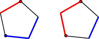
Figure 1: There are two possible scenarios corresponding to case where there is at least one integer and one non-integer solution (case 3 in the proof). The two-term inequalities decide the values for two $x_{i}$s and have been represented as edges and nodes (highlighted as small circles) have been used to denote the values determined by the one-term inequalities. Depending on the way the combination of inequalities is selected, one gets either all $x_{i}$s as integers or a redundant set of inequalities leading to an undecidable value for $x_{i}$s.

We end by showing that the FCNC inequality is facet defining (in the exclusivity graph approach). All incidence vectors (we will restrict to the ones corresponding to the stable set of the $n$ cycle graph, for this proof) will always satisfy the FCNC inequality because the cardinality of the stable set is bounded by the independence number (see LABEL:Def:independenceNumber in SM) of the graph, which for our case is $\left(n-1\right)/2$ (Knuth, 1994; Bengtsson, 2009; Liang et al., 2011). We will now show that there are exactly $n$ vertices of STAB, i.e. incidence vectors which saturate the said inequality. To saturate, the incidence vector must have $\left(n-1\right)/2$ components with entry $1$, and the remaining $\left(n+1\right)/2$ components with entry $0$. Note that each incidence vector satisfies the STAB inequalities, i.e. if a given component is $1$ then its adjacent components are necessarily $0$. One can convince themselves that any such vector, i.e. incidence vectors that saturate the FCNC inequality, must have two zeros adjacent (cyclically over $n$) while all other entries are alternatively one and zero. The total number of ways of placing two adjacent zeros, which is exactly $n$, then gives us the total number of incidence vectors which saturate the inequality thereby proving that the FCNC inequality is indeed facet defining.

∎

IV Uniqueness of fundamental anti-cyclic inequalities

We show that the odd anti-cycle admits a unique inequality. This follows easily from the following known result. For any set of nonnegative vectors $X$, its antiblocker is defined as

$$\text{abl }X=\left\{y\geq 0:x.y\leq 1\;\forall\>x\in X\right\}.$$

Let us denote by $\bar{G}$ the complement graph of $G$, viz. $\bar{G}=\left\{V,\bar{E}\right\}$ if $G=\left\{V,E\right\}$, which in particular means that if $G$ is a cyclic graph, then $\bar{G}$ is an anti-cyclic graph.

Lemma 3.

For any graph $G$ we have

$$\text{STAB}(\bar{G}) =\text{abl }\text{QSTAB}(G)$$

$$\text{TH}(\bar{G}) =\text{abl }\text{TH}(G)$$

$$\text{QSTAB}(\bar{G}) =\text{abl }\text{STAB}(G).$$

Note that $\text{abl }X=\text{abl }\text{convex hull }X$ because every element $y\in\text{abl }X$ will satisfy $\left(\theta_{1}x_{1}+\dots+\theta_{k}x_{k}\right).y\leq 1$ where $\sum_{i=1}^{k}\theta_{i}=1$.

Theorem 2.

Let $G$ be odd $n$-cycle graph $(n>3)$and consider the exclusivity graph scenario associated with $\bar{G}$. There is a unique facet-defining NC inequality, given by $\sum_{i=1}^{n}p_{i}\leq 2$.

Proof.

We characterise $\text{QSTAB}(\bar{G})$ and $\text{STAB}(\bar{G})$ by using LABEL:Lem:antiBlocker. Let $\{v_{1},v_{2}\dots v_{n}\}$ denote the vertices of $\text{STAB}(G)$. Each vertex $v_{i}$ corresponds to a hyperplane constraining $\text{abl }\text{STAB}(G)=\text{QSTAB}(\bar{G})$. From the proof of LABEL:Thm:main we know that $\text{QSTAB}(G)$ has exactly one more vertex, call it $v_{0}$. Corresponding to $v_{0}$ there will be exactly one extra hyperplane constraining $\text{abl }\text{QSTAB}(G)=\text{STAB}(\bar{G})$ compared to those constraining $\text{abl }\text{STAB}(G)=\text{QSTAB}(\bar{G})$. This hyperplane is precisely $\sum_{i=1}^{n}p_{i}\leq 2$ using $v_{0}=\left(1/2,1/2,\dots 1/2\right)$ and the definition of the anti-blocker. ∎

V Discussion and Conclusion

We showed that all fundamental NC inequalities are unique for their corresponding odd cycle (or anti-cycle) exclusivity scenario. This is an exponential simplification compared to the compatibility hypergraph scenario (see LABEL:Sec:Relative-Simplification-Explaine). Any exclusivity scenario witnessing contextuality will have associated with it at least one fundamental NC inequality but there may be others; we give an example of this using the simplest Bell exclusivity scenario (report a new Bell inequality in the process; see LABEL:Sec:All-Bell-Inequalities). All polytopes associated with these scenarios can also be seen to admit the same geometric interpretation which is discussed in LABEL:Sec:Geometric-Representation of SM.

A possible future direction would be to link our results to the resource theory of contextuality. The simplification for cyclic and anti-cyclic exclusivity scenarios indicates that there is a unique way to capture the amount of contextuality, to wit, distance of the contextual behaviour from the hyperplane corresponding to fundamental NC inequalities. The perfect graph theorem could potentially allow a generalisation to all exclusivity scenarios.

VI Acknowledgement

We are thankful to Michael Kleder for the CON2VERT and VERT2CON MATLAB packages that gave us the first numerical glimpse of our result.

ASA and JR acknowledge the financial support from the Belgian Fonds de la Recherche Scientifique - FNRS under grants no F.4515.16 (QUICTIME), R.50.05.18.F (QuantAlgo). ASA further acknowledges the FNRS for support through the grant F3/5/5–MCF/XH/FC–16749 FRIA. KB acknowledges the CQT Graduate Scholarship. KB and LCK are grateful to the National Research Foundation and the Ministry of Education, Singapore for financial support.

Appendix A All Bell Inequalities for the Simplest Exclusivity Graph

Given a list $[L$] of integers, a graph with $n$ vertices where every $i$-th vertex is connected to every other $(i+l)$ mod $n$-th vertices for $l\in[L]$ is called a circulant graph $\text{Ci}_{n}[L].$ The exclusivity graph corresponding to the measurement events for CHSH inequality is a circulant graph. In particular, it is represented as $\text{{Ci}}_{8}[1,4]$ graph. This is the simplest exclusivity graph which can lead to Bell inequalities if one analyses the corresponding stable set polytope (Sadiq et al., 2013).

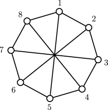
Figure 2: CHSH inequality is a unique non-trivial facet defining NC inequality for $(2,2,2)$Bell scenario. The measurement events which are employed to get the CHSH inequality follow the exclusivity relations according to $\text{{Ci}}_{8}[1,4]$ graph.

We ran numerical tests to characterize the convex polytope STAB($\text{{Ci}}_{8}[1,4]$) and found three types of non-trivial facets.

1. Pentagonal inequalities: There are eight such inequalities and correspond to eight induced pentagons (five cycles). In the literature, these are known as pentagonal Bell inequalities (Sadiq et al., 2013). Formally, the pentagonal inequalities are given by

   $$\sum_{i=k}^{(k+4)\text{mod}8}p_{i}\leq 2$$

   for $k\in\{1,2,3,4,5,6,7,8\}.$

2. Heptagonal inequalities: There are eight such inequalities and correspond to induced sugraphs of $\text{{Ci}}_{8}[1,4]$ with any seven nodes. These inequalities have not been reported earlier to the best of our knowledge. Formally, the heptagonal NC inequalities are given by

   $$\sum_{i=k}^{(k+6)\text{mod}8}p_{i}\leq 3$$

   for $k\in\{1,2,3,4,5,6,7,8\}.$

3. CHSH inequality: The CHSH inequality corresponds to sum of the probabilities of all eight events and is formally given by

   $$\sum_{i=1}^{8}p_{i}\leq 3.$$

Note that neither the Heptagonal inequalities nor the CHSH inequality correspond to any odd-cycle (or its complement).

Appendix B Geometric Representation

Figure 3: Two conceivable illustrations of the QSTAB polytope (light blue) and the KCBS inequality (black) separating the said polytope from the STAB polytope. In the left image, the vertices of both polytopes are the same (except one) but there are two facets of QSTAB which are not a facet of STAB. One can show that all the facets of QSTAB are also the facets of STAB. This rules out the first image. The second image illustrates an alternative which helps us intuitively understand the higher dimension underlying geometry.

Fix an odd $n>3$. Geometrically, the FCNC inequality corresponds to a unique hyperplane cutting through QSTAB which separates all E-principle behaviours (see LABEL:Def:ePrincipleBehaviour in Supplementary Material (SM)) uniquely into two parts, namely non-contextual and contextual. Naïvely one might imagine the QSTAB polytope and the FCNC inequality to geometrically be illustrated by the image on the left in LABEL:Fig:Two-conceivable-illustrations. However, it is not too hard to show that all the facets of QSTAB are also the facets of STAB which means the naïve understanding is flawed. The image on the right in LABEL:Fig:Two-conceivable-illustrations better illustrates the geometry of the two convex polytopes (STAB and QSTAB). Recall that STAB for a given graph is identical to the anti-blocker of QSTAB for the complement graph and similarly QSTAB for a given graph is identical to the anti-blocker of STAB for the complement graph (see LABEL:Lem:antiBlocker in MT). We thus recover essentially the same geometry for the anti-cyclic exclusivity scenario. In summary, given an $n$-cyclic (or anti-cyclic) exclusivity scenario, the associated fundamental NC inequality separates the corresponding E-principle behaviours into parts and uniquely singles out a vertex corresponding to the maximally contextual behaviour.

Appendix C Relative Simplification Explained

Where is this exponential simplification coming from and are we losing something in the process? To answer these questions we connect the inequality we obtained using the exclusivity graph approach to the one obtained using the compatibility hypergraph approach. We briefly introduce the compatibility hypergraph approach first (deferring a complete description to LABEL:Sec:Compatibility-Hypergraph-Approac).

C.1 Compatibility Hypergraph Approach | Overview

Instead of looking at the exclusivity of events, the compatibility hypergraph approach is based on, as the name suggests, the compatibility of measurements. The scenario here is defined by a hypergraph $G$, where the vertices $V(G)$ represent the measurements and the hyperedges $\mathcal{C}(G)$ of the graph represent the set of measurements which are compatible (see Definitions 33 and 34 in SM). The set of nodes/measurements in a hypergraph constitute a context (see Definition 10 in SM). For each context $C\in\mathcal{C}$, a normalised probability vector $p_{C}$, is defined which assigns probabilities to every possible joint outcome corresponding to the measurements belonging to that context (see Definition 10 in SM). The behaviour $p$, in this formalism, is defined to be the concatenation of all these probability vectors (one vector for each context; see Definition 37 in SM). Consider a fixed measurement. The behaviours which assign the same marginal probability distribution to the outcomes corresponding to this measurement, regardless of which probability vector (and hence context) was used to evaluate the marginal, are said to be non-disturbing behaviours. The set of such behaviours happens to be a convex polytope and is denoted by $\mathscr{X}(G)$ (pronounced as $X$; see Definition 40 in SM). It is analogous (and reduces, under the appropriate restrictions) to the no-signalling distributions. Consider the set of behaviours which arise by associating a quantum observable with each measurement such that the compatibility requirements are satisfied. This set is called the set of quantum behaviours $\mathscr{Q}(G)$ and it happens to be convex. Finally, consider behaviours which admit a non-contextual completion (see Definition 12 in SM). These behaviours can be equivalently characterised as behaviours which arise from a global joint distribution over all the observables such that the marginals yield the various probability vectors constituting the behaviour (see Theorem 3 in SM). These define the set of classical behaviours $\mathscr{C}(G)$ which, like $\mathscr{X}(G)$, happens to be a convex polytope. The facet-defining hyperplanes of $\mathscr{C}(G)$ yield NC inequalities.

C.2 The KCBS inequality

For concreteness, we consider the KCBS scenario in the compatibility hypergraph formalism. Let $\{M_{0},M_{1},M_{2},M_{3},M_{4}\}$ be five dichotomic measurements, which form the set of vertices $V(G)$, and let $\{M_{0},M_{1}\},\{M_{1},M_{2}\},\{M_{2},M_{3}\},\{M_{3},M_{4}\},\{M_{4},M_{0}\}$ denote the compatibility relations among them $\mathcal{C}(G)$, which define the (hyper)edges. This results in $G$ being a $5$-cycle (hyper)graph (see LABEL:Fig:KCBS_compatibility_hypergraph). It would be helpful to use two different conventions for labelling the outcomes of the measurements: binary $(0,1)$ and signed $(+1,-1)$. In the binary convention, the probability of obtaining the outcome $(0,0)$ upon the measurement of $M_{i}$ and $M_{i+1}$ is denoted by $p_{i,i+1}(00)$. This is consistent with our notation for the probability vector $p_{C}$ where $C$ was the context, which in this case is denoted by $i,i+1$. The addition in the indices is modulo $5$. Similarly in the signed convention, the outcome $(+1,+1)$ is denoted by $p_{i,i+1}(++)$. Further, to represent the expectation value of the product of measurements $M_{i}M_{i+1}$ we use the notation

$$\left\langle i,i+1\right\rangle =p_{i,i+1}(++)+p_{i,i+1}(--)$$ (5)

$$\;\;-p_{i,i+1}(+-)-p_{i,i+1}(-+).$$

Note that we discuss expectation values only in the signed convention. By studying the polytope of classical behaviours $\mathscr{C}(G)$ one can find the facet-defining hyperplanes which yield the NC inequalities. These turn out to be (Araújo et al., 2013)

$$\gamma_{0}\left\langle 0,1\right\rangle+\gamma_{1}\left\langle 1,2\right\rangle+\gamma_{2}\left\langle 2,3\right\rangle+\gamma_{3}\left\langle 3,4\right\rangle+\gamma_{4}\left\langle 4,0\right\rangle\leq 3$$

where $\gamma_{i}\in\{\pm 1\}$ such that the number of $\gamma$s with a negative sign are odd. To see how these relate to the unique KCBS inequality we obtain using the exclusivity graph approach, consider the possible events corresponding to a given context ((hyper)edge). All these events are mutually exclusive because they correspond to different outcomes of a given set of measurement (see LABEL:Fig:ExclusivityFromCompatibility). This exclusivity is denoted by the ellipse in the graph. Now consider the measurement $M_{0}$. Let $(01|M_{0}M_{1})$ denote the event where $M_{0}$ and $M_{1}$ are measured and the outcomes are $0$ and $1$ respectively ( see Definitions 13 and 14). Using this notation, observe that the events $(01|M_{0}M_{1})$, $(00|M_{0}M_{1})$, $(11|M_{4}M_{0})$ and $(01|M_{4}M_{0})$ are mutually exclusive. The first two are exclusive as they correspond to different outcomes of $M_{1}$, the second and third are exclusive because they correspond to different outcomes of $M_{0}$, the third and fourth are exclusive because they correspond to different outcomes of $M_{4}$. A similar argument works for all the other pairs. This exclusivity is denoted by a straight line. One can verify that all the events on a given straight line are exclusive. If we let $e_{i}=(01|M_{i}M_{i+1})$ then a 5-cycle exclusivity graph can be extracted from the aforementioned by defining the set of vertices to be the set of events $\{e_{0},e_{1},\dots e_{4}\}$ and the set of edges to be their exclusivity relations $\{\left\{e_{0},e_{1}\right\},\left\{e_{1},e_{2}\right\}\dots,\left\{e_{4},e_{0}\right\}\}$. We had denoted the probability of these events by $p_{i}$ to write the KCBS inequality, which in our current notation, becomes

$$p_{0,1}(01)+p_{1,2}(01)+p_{2,3}(01)+p_{3,4}(01)+p_{4,0}(01)\leq 2.$$ (6)

Since the exclusivity graph approach doesn’t require the explicit specification of the measurements which lead to exclusivity, merely their existence, it is able to extract the essential nature of the problem without creating redundancies caused by the labelling. If the complete exclusivity graph was used then the exclusivity graph formalism should yield effectively the same NC inequalities as the compatibility hypergraph approach, recreating the said redundancies . We now explicitly combine the following two NCinequalities obtained using two different exclusivity graphs,

$$\sum_{i=0}^{4}p_{i,i+1}(01)\leq 2,\;\sum_{i=0}^{4}p_{i,i+1}(10)\leq 2,$$

into an NC inequality obtained using the compatibility hypergraph formalism,

$$-\sum_{i=0}^{4}\left\langle i,i+1\right\rangle\leq 3,$$ (7)

which corresponds to taking all $\gamma_{i}=-1$. Using $p_{i,i+1}(00)=p_{i,i+1}(++)$ (which holds by assumption; they were just different labels for the same outcomes) in LABEL:Eq:Exp(ij), and probability conservation (probability vectors $p_{C}$ are normalised; in a given context, the probabilities sum to one) we deduce

$$\left\langle i,i+1\right\rangle=1-2(p_{i,i+1}(01)+p_{i,i+1}(10)).$$ (8)

To obtain LABEL:Eq:KCBScompatibilityAllMinus we sum the two inequalities

$$\sum_{i=0}^{4}\left(p_{i,i+1}(01)+p_{i,i+1}(10)\right) \leq 4$$

$$\iff\sum_{i=0}^{4}\underbrace{\left(2p_{i,i+1}(01)+p_{i,i+1}(10)-1\right)}_{=-\left\langle i,i+1\right\rangle} \leq 8-5=3.$$

While at first sight, it might appear that the inequality obtained using the compatibility hypergraph is weaker as it is a linear combination of two exclusivity graph based inequalities, this conclusion is incorrect. This is because we can do better. We can obtain from a single compatibility hypergraph based inequality a corresponding exclusivity graph based inequality. We show this explicitly for $\sum_{i=0}^{4}p_{i,i+1}(01)\leq 2$. The marginal $p_{i}(1)=\sum_{l=0}^{1}p_{i,j}(1l)$ for every $i,j$ belonging to a hyperedge. We start with noting that $p_{i,i+1}(10)+p_{i,i+1}(01)=p_{i}(1)-p_{i,i+1}(11)+p_{i,i+1}(01)$ but we can also write $p_{i}(1)=p_{i-1,i}(01)+p_{i-1,i}(11)$ (this is a consequence of the no-disturbance requirement). Consequently, using LABEL:Eq:CorrTo01, we have

$$1-\left\langle i,i+1\right\rangle =2\Big{(}p_{i-1,i}(01)+p_{i-1,i}(11)$$

$$\;\;-p_{i,i+1}(11)+p_{i,i+1}(01)\Big{)}$$

$$\implies 5-\sum_{i=0}^{4}\left\langle i,i+1\right\rangle =4\sum_{i=0}^{4}p_{i,i+1}(01)$$

and substituting LABEL:Eq:KCBScompatibilityAllMinus we obtain $4\sum_{i=0}^{4}p_{i,i+1}(01)\leq 5+3$ which is just LABEL:Eq:exclusivityKCBSinCompatibilityLikenotation.

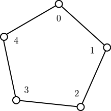
(a) KCBS in the compatibility hypergraph approach

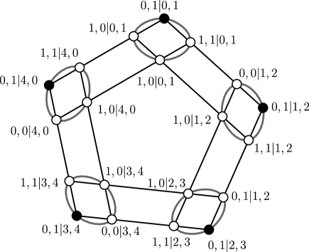
(b) Exclusivity graph arising from the KCBS compatibility hypergraph.

Figure 4: Relation between the KCBS exclusivity and compatibility graphs

[The NC inequalities for the compatibility hypergraph structure corresponding to anti-cycles is not known in the literature. A numerical investigation for the classical polytope for the same indicates the presence of exponentially many non-trivial NC inequalities. However in the exclusivity graph approach, the non-trivial NC inequalities corresponding to anti-cycles are unique (see Theorem ref). The reason for the simplification is same as the cyclic case.

Appendix D Probabilistic Models | States and Measurements

The results discussed here are based on the work of Amaral and Cunha (2018). In any experimental scenario there are two types of interventions possible, either preparation or operation. Preparation is used in the intuitive sense of the word, that is preparing the system in a given state, for instance using a laser to initialise the state of an atom. More explicitly, we make the following assumptions about the theory.

• Interventions are of two types: Preparation and Operation.

• Experiments are reproducible: For each operation, there may be several different outcomes, each occurring with a well defined probability for a given preparation.

Definition 1 (State).

Two preparations are defined to be equivalent if they give the same probability distribution for all available operations. We will refer to the equivalence class of preparations as state.

Definition 2 (State space).

The set of all states is referred to as the state space of the system.

Remark 1.

The state space is convex.

Definition 3 (Pure states).

All extremal points of the state space are defined to be pure states.

Definition 4 (Measurements).

Measurements are operations with more than one outcome.

Remark 2.

Unitary evolution is an example of an operation which is not a measurement.

Definition 5 (Probabilistic model).

We call any mathematical description of a physical system which provides the following, a probabilistic model.

1. Objects to represent

   1. state

   2. operations

   3. measurements

2. Rule to calculate the probabilities of the possible outcomes of any arbitrary measurement given any arbitrary state.

Definition 6 (Probability theory).

A probability theory is a collection of probabilistic models.

Definition 7 (Outcome repeatable measurements).

A measurement $j$ is defined to be an outcome repeatable measurement if every time one performs this measurement on a system and an outcome $k$ is obtained, a subsequent measurement of $j$ on the same system gives the outcome $k$ again with probability one.

Definition 8 ($p_{j}(k)$).

The probability of getting an outcome $k$ given that a measurement $j$ has been performed will be denoted by $p_{j}(k)$.

All the measurements henceforth will be assumed to be outcome-repeatable.

Definition 9 (Compatible measurements, refinement and coarse graining).

A set of measurements $\{j_{1},j_{2}\dots j_{n}\}$ is compatible if there is another measurement $j$ with outcomes $\{1,\dots m\}$ and functions $\{f_{1},f_{2}\dots f_{n}\}$ such that the possible outcomes of $j_{s}$ is the same as $\left\{f_{s}(1),f_{s}(2)\dots f_{s}(m)\right\}$ for each $s$ and

$$p_{j_{s}}(l)=\sum_{k\in f_{s}^{-1}(l)}p_{j}(k)$$

where $j$ is called a refinement of $\{j_{1},j_{2}\dots j_{n}\}$ and each $j_{s}$ is called a coarse graining of $j$.

If a set of measurements is compatible it is called a set of compatible measurements.

Completion of a probabilistic model

Definition 10 (Context).

A set of compatible measurements is defined to be a context.

Our objective now is to construct a general mathematical framework which can describe the completion of a probabilistic model, i.e. give a model which is no longer probabilistic but reduces to the same probabilistic model if certain variables are ignored.

Definition 11 (Completion).

Consider a probabilistic model $P$ where $S$ represents the set of pure states and $X$ represents the set of measurements. The completion of this probabilistic model, denoted by $P^{\prime}$, consists of a set of measurements $X^{\prime}$, which are in one-to-one correspondence with $X$, and a set of pure states $S^{\prime}$, which are in one-to-one correspondence with $\Lambda\times S$ for some set $\Lambda$. $P^{\prime}$ must satisfy the following requirements. For all $\rho\in S$ and all contexts $c=\{j_{1},j_{2}\dots j_{n}\}$, $P^{\prime}$ should specify a probability distribution over $\Lambda$ given by $p(\lambda)$ and a probability distribution $p_{j_{k}}^{(\lambda,\rho,c)}:\mathbb{R}\to\{0,1\}$ for each $\lambda,\rho,c,j_{k}$ such that

$$p_{c}^{\rho}(i_{1},i_{2}\dots i_{m})=\sum_{\lambda\in\Lambda}p(\lambda)\prod_{k=1}^{m}p_{j_{k}}^{(\lambda,\rho,c)}(i_{k})$$

where $p_{c}^{\rho}(i_{1},i_{2}\dots i_{m})$ is the probability assigned by $P$ to the measurement of $j_{1},j_{2}\dots j_{n}$ (encoded in $c$) yielding the outcomes $i_{1},i_{2}\dots i_{m}$, respectively, for the state $\rho$.

Remark 3.

We expect the completion $P^{\prime}$ to specify $S^{\prime}$ as $(\lambda,\rho)$ for all $\lambda\in\Lambda$ and $\rho\in S$. Let us assume for simplicity that $X^{\prime}=X$. Now for every context $c=\{j_{1},j_{2}\dots j_{n}\}$ (i.e. set of compatible measurements from $X$) the completion $P^{\prime}$ will predict with certainty the outcome of measuring any $j_{i}\in c$, for a given $(\lambda,\rho)$. This prediction is allowed to depend on the set $c$ itself to accommodate “contextual completions”. We will see later that non-contextual (and functionally consistent) completions contradict the predictions of quantum mechanics.

Let $X$ be a set of measurements. Let $\{j_{1},j_{2}\dots j_{m}\}\subset X$ be a set of compatible measurements.

Definition 12 (Non-contextual completion).

Let $c_{1}=\left\{j_{1},j_{2},\dots j_{m}\right\}$, $c_{2}=\left\{j_{1},j_{2}^{\prime},\dots j_{m}^{\prime}\right\}$ be two contexts (note that $j_{i}$ and $j_{k}^{\prime}$ may not be compatible for $i,k>1$). A completion $P^{\prime}$ of a probabilistic model $P$ is called non-contextual if $p_{j_{1}}^{(\lambda,\rho,c_{1})}(i)=p_{j_{1}}^{(\lambda,\rho,c_{2})}(i)$ for all contexts $c_{1}$ and $c_{2}$ of the aforesaid form.

Appendix E The Exclusivity Graph Approach

E.1 Formalising Scenarios

Suppose Let $(a_{1},a_{2}\dots|M_{1},M_{2}\dots)$

Definition 13 (Measurement event).

We denote a measurement event by $(a_{1}a_{2}\dots a_{n}|M_{1}M_{2}\dots M_{n})$ where $a_{i}$ is the measurement outcome associated with $M_{i}$, and $M_{i}$ is compatible with $M_{j}$ for all $i,j\in\{1,2\dots n\}$. Two measurement events $(a_{1}a_{2}\dots a_{n}|M_{1}M_{2}\dots M_{n})$ and $(a|M)$ are equivalent if for all states (see LABEL:Def:state), their probabilities of occurrence of these events are equal.

For brevity, we will use the word event in lieu of equivalent measurement events whenever there is no ambiguity.

Definition 14 (Exclusive event).

Two events $e_{i}$ and $e_{j}$ are defined to be exclusive if there exists a measurement $M$ such that $e_{i}$ and $e_{j}$ correspond to different outcomes of $M$, i.e. $e_{i}=(a_{i}|M)$ and $e_{j}=(a_{j}|M)$ such that $a_{i}\neq a_{j}$.

Definition 15 (Exclusivity graph).

For a family of events $\{e_{1},e_{2}\dots e_{n}\}$ we associate a simple undirected graph, $G:=(V,E)$, with vertex set $V$ and edge set $E$ such that two vertices $i,j\in V$ share an edge if and only if $e_{i}$ and $e_{j}$ are exclusive events. $G$ is called an exclusivity graph.

Definition 16 (Probability vector).

For a given exclusivity graph $G=(V,E)$ and a probability theory, the probability vector is a vector $p\in\mathbb{R}^{\left|V\right|}$ such that $p_{(i)}=\text{prob}(e_{i})$ where $\text{prob}(e_{i})$ is the probability assigned by the probability theory to the event $e_{i}$.

Definition 17 (Behaviour).

A behaviour for an exclusivity graph $G=(V,E)$ is a map $p:V\to\left[0,1\right]$ which assigns to each vertex $i\in V$ a probability $p(i)$ such that $p(i)+p(j)\leq 1$, for all vertices that share an edge, i.e. $\left(i,j\right)\in E(G)$. Due to the isomorphism between the map $p:V\to[0,1]$ and the vector $\vec{p}\in\{0,1\}^{\left|V\right|}$ we will associate with the $i^{\text{th}}$ component of $\vec{p}$ the value $p(i)$, i.e. $\vec{p}_{(i)}=p(i)$. (Sometimes we will even drop the vector sign.)

Remark 4.

We don’t use $p_{(i)}=p_{M}(i)$ because $M$ is not explicitly, a priori known so cluttering the notation doesn’t help.

Definition 18 (Non-contextual behaviour).

A behaviour $p$ is called a deterministic non-contextual behaviour if $p:V\to\{0,1\}$, i.e. $p_{(i)}\in\{0,1\}$ for all $i$ and there exists a non-contextual completion of the corresponding probabilistic model $P$. The set of non-contextual behaviour is defined to be the convex hull of deterministic non-contextual behaviours and is denoted by $B_{\text{NC}}(G)$.

Remark 5.

Defining the behaviour this way implicitly imposes functional consistency. This is because we require a non-contextual completion of deterministic behaviours to start with and later take its convex combination. This imposes the exclusivity condition at the level of the hidden variable model which in turn is a manifestation of functional consistency.

Definition 19 (Quantum behaviour).

A behaviour for an exclusivity graph $G$ is called a quantum behaviour if there exists a quantum state $\rho$ and projectors $\Pi_{1},\dots\Pi_{n}$ acting on a Hilbert space $\mathcal{H}$ such that $p_{(i)}=\text{Tr}(\rho\Pi_{i})$ for all $i\in V$ and $\text{Tr}(\Pi_{i}\Pi_{j})=0$ for vertices that share an edge, i.e. $(i,j)\in E$.

The convex set of all quantum behaviours is denoted by $B_{Q}(G)$.

Definition 20 (The exclusivity principle).

Given a subset $\{e_{i}\}$ of events which are pairwise exclusive we say that the exclusivity principle is obeyed by a probabilistic model if $\sum_{i}\text{prob}(e_{i})\leq 1$ for all such subsets. We will sometimes refer to this as the E-principle.

Definition 21 (E-principle behaviour).

A behaviour $p$ for an exclusivity graph $G$ is said to be an E-principle behaviour if the associated probabilistic model satisfies the exclusivity principle, i.e. $\text{prob}(e_{i})=p_{(i)}$ satisfies the E-principle.

The set of E-principle behaviours will be denoted by $B_{E}(G)$.

Let $e_{1},e_{2}\dots e_{n}$ denote a family of measurement events.

Remark 6.

The set $B_{\text{NC}}(G)$ is a (convex) polytope, i.e. can be expressed as a solution of a finite number of linear inequalities.

Definition 22 (NC inequality, facet-defining).

Let $p$ be a behaviour and $\gamma_{i},\beta\in\mathbb{R}$. A linear inequality, $\sum\gamma_{i}p_{(i)}\leq\beta$, is called an NC inequality of its satisfaction is a necessary condition for membership to the set $B_{\text{NC}}(G)$. Equivalently, to claim non-membership in the set $B_{\text{NC}}(G)$, it is sufficient to show a violation of the said linear inequality.

An NC inequality is called facet-defining if it defines a non-trivial facet of $B_{\text{NC}}(G)$.

E.2 Lovász Geometry

At the risk of causing frustration by redundancy, we state the following for clarity.

Definition 23.

Graph: $G=(V,E)$ defined by the set of vertices and the set of edges.

Definition 24.

Orthonormal representation w.r.t. a graph $G$ is defined as follows. For all $i\to\left|v_{i}\right\rangle$ in $\mathbb{R}^{d}$ such that $\left\langle v_{i}|v_{j}\right\rangle=0$ whenever $(i,j)\notin E$.

Definition 25.

For a vector $\left|v_{i}\right\rangle$ in an orthonormal representation, the cost is defined as

$$c_{i}=\left|\left\langle\psi|v_{i}\right\rangle\right|^{2}$$

where $\left|\psi\right\rangle\doteq\left(1,0,\dots,0\right)$ is a vector in $\mathbb{R}^{d}$.

Definition 26.

The theta body corresponding to a graph $G$ is defined to be

$$\text{TH}(G)=\left\{p\in\mathbb{R}^{\left|V\right|}\Big{|}p_{(i)}=c_{i}\right\}$$

where $c_{i}$ is the cost (see LABEL:Def:costOfVector) corresponding to $\bar{G}:=\left(V,\bar{E}\right)$.

Definition 27.

Stable set/Independent set is a subset of vertices $K\subseteq V$ such that for all $i,j\in K$ there is no edge between $i$ and $j$, viz. $(i,j)\notin E$.

Definition 28.

Independence number of a graph $G$ is defined to be the cardinality of the largest independent set of $G$.

Definition 29.

Clique is a subset of vertices $K\subseteq V$ such that for all $i,j\in K$ there is an edge between $i$ and $j$, viz. $(i,j)\in E$.

Definition 30.

Incidence vector of a set is defined to be a vector $\vec{p}$ (of size $\left|V\right|$) for $K\subseteq V$ such that

$$p_{(i)}=\begin{cases}1&\text{if }i\in K\\ 0&\text{else}.\end{cases}$$

Example 1.

Consider the $5$-cycle graph $V=\left\{1,2,3,4,5\right\}$, $E=\{(1,2),(2,3),(3,4),(4,5),(5,1)\}$. $K=\{1,3\}$ is an example of a stable set. $K^{\prime}=\{1,2\}$ is an example of a clique. The incident vector corresponding to $K$ is $p=(1,0,1,0,0)^{T}$.

Definition 31.

STAB($G$) (not to be confused with the stable set) is defined as the convex hull of the vectors $\vec{p}_{(k)}$ for all stable sets $k$ where $\vec{p}_{(k)}$ is the incidence vector of the set $k$. (Note: if $k$ were an index, $\vec{p}_{(k)}$ would refer to the $k^{\text{th}}$ component of the vector $\vec{p}$; here $k$ is a set).

Definition 32.

QSTAB($G$) is the set of vectors $x\in\mathbb{R}^{\left|V\right|}$ such that $x_{i}\geq 0$, $\sum_{i\in Q}x_{i}\leq 1$ for every clique $Q$.

Lemma 4.

(Grötschel et al., 2011) STAB($G$) is the convex hull of the integer-solutions to the equations $x_{i}\geq 0$, $\left(x_{i}+x_{j}\right)\leq 1$ for every $(i,j)\in E$, where $G=(V,E)$.

Remark 7.

Every set of indices which is an edge is also a clique (the other way is not necessary, obviously). This means that the inequalities listed in LABEL:Def:QSTAB (viz. $\sum_{i\in Q}x_{i}\leq 1$ for every clique $Q$) contain the inequalities listed in LABEL:Lem:STAB (viz. $x_{i}+x_{j}\leq 1$ for every $(i,j)\in E$).

Lemma 5.

(Knuth, 1994) STAB(G)$\subseteq$TH(G)$\subseteq$QSTAB(G).

E.3 Impossible Completions | Linking geometry and quantum mechanics

Lemma 6.

(Cabello et al., 2014) Let $e_{1},e_{2}\dots e_{n}$ be the (exclusive) events associated with an Exclusivity Graph $G=(V,E)$. Then,

$$B_{\text{NC}}(G) =\text{STAB}(G),$$

$$B_{Q}(G) =\text{TH}(G),$$

$$B_{E}(G) =\text{QSTAB}(G).$$

Corollary 1.

For a given Exclusivity Graph $G$ we have

$$B_{\text{NC}}(G)\subseteq B_{Q}(G)\subseteq B_{E}(G).$$

Appendix F Compatibility Hypergraph Approach

F.1 Formalising Scenarios

Definition 33 (Compatibility Scenario).

A compatibility scenario is specified by the tuple $\Upsilon:=(X,\mathcal{C},O)$ where

• $O$ is a finite set.

• $X$ is a finite set of random variables from $O$ to $\mathscr{P}(O)$.

• $\mathcal{C}$ is a collection of subsets of X such that their union is equal to X and the intersection of any two subsets is never equal to one of the subsets. Each of these subsets will be called a context.

It might be useful to keep the following in mind to get an intuitive understanding. The set $X$ can be thought of as the measurements, the set $O$ as the outcome of these measurements, and the set $\mathcal{C}$ as containing maximal contexts. [rephrase]

Definition 34 (Compatibility Hypergraph).

The compatibility hypergraph corresponding to a scenario $\Upsilon:=(X,\mathcal{C},O)$ is a hypergraph whose nodes are elements in $X$ and hyperedges are contexts in $\mathcal{C}$. We denote the compatibility hypergraph for the scenario by $\mathcal{H}=(X,\mathcal{C})$.

We use calligraphic letters to notationally distinguish the (hyper)graphs associated with the compatibility hypergraph from those associated with the exclusivity graph approach.

Definition 35 (Compatibility Graph).

The compatibility graph for a scenario is the $2$-skeleton of the corresponding hypergraph i.e. $\mathcal{H}=(X,\mathcal{C})$. We will denote the compatibility graph by $\mathcal{G}=(X,E).$ Given two elements $i$ and $j$ in $X$, they share an edge in $E$ iff $\{i,j\}\subseteq C$ for some context $C\in\mathcal{C}.$

Definition 36 (Measurement Event).

A measurement event corresponds to a single run of an experiment where the measurements in a context $C\in\mathcal{C}$ are jointly performed with outcomes in $O^{\left|C\right|}.$

Henceforth, for notational simplicity, we use $O^{C}$ instead of $O^{\left|C\right|}$.

Definition 37 (Behaviour and Behaviour Vector).

Given a scenario $\Upsilon:=(X,\mathcal{C},O)$, a behaviour is a family of probability distributions defined over $O^{C}$, defined as

$$B=\left\{p_{C}:O^{C}\to[0,1]\Big{|}\sum_{s\in O^{C}}p_{C}(s)=1,C\in\mathcal{C}\right\}.$$

One can stack the $p_{C}(s)$ for all $s\in O^{C}$ and $C\in\mathcal{C}$ to form a column vector of probabilities for a behaviour $B$. Such probability vectors are called behaviour vectors.

Remark 8.

The set of possible behaviours forms a polytope with $\prod_{C\in\mathcal{C}}\left|O^{C}\right|$ nodes, where the extreme points (nodes) correspond to deterministic points i.e. $p_{C}(s)$ equal to $0$ or 1. This can be deduced from the convexity of probability distributions.

Definition 38 (Restriction Map).

Given a context $C\in\mathcal{C}$ with outcomes in $O^{C}$ and a set $U\subset C,$ a restriction map $r_{U}^{C}$ is given by

$$r_{U}^{C}:O^{C}\rightarrow O^{U},$$

$$s=\left(a_{i}\right)_{M_{i}\in C}\mapsto s|_{U}=\left(a_{i}\right)_{M_{i}\in U}.$$

Definition 39 (Marginal Distribution (for a context)).

The marginal distribution for a probability distribution over a context $C\in\mathcal{C}$ corresponding to a set $U\subset C$ is defined as

$$p_{U}^{C}:O^{U}\rightarrow[0,1],$$

$$p_{U}^{C}(s)=\sum_{s^{\prime}\in O^{C};r_{U}^{C}(s^{\prime})=s}p_{C}(s^{\prime}),$$

where $r_{U}^{C}$ is a restriction map from $O^{C}$ to $O^{U}.$

Definition 40 (Non-disturbing Set, $\mathscr{X}(\Upsilon)$).

Given a scenario $\Upsilon:=(X,\mathcal{C},O)$, the set of behaviours is called non-disturbing set, if for any given behaviour and two different context $C_{1}$and $C_{2}$, we have $p_{C_{1}\cap C_{2}}^{c_{1}}=p_{C_{1}\cap C_{2}}^{c_{2}}.$

Definition 41 (Global Section).

Given a scenario $\Upsilon:=(X,\mathcal{C},O)$, a global section for $X$ is a probalility distribution over $O^{X},$denoted by $p_{X}:O^{X}\rightarrow[0,1].$

Definition 42 (Global Section for a behaviour).

Given a scenario $\Upsilon:=(X,\mathcal{C},O)$ and a behaviour $B$, a global section $p_{X}$ is called a global section for the behaviour $B$ if

$$p_{C}^{X}=p_{C}\quad\forall\quad C\in\mathcal{C}.$$

Definition 43 (Non-contextual Behaviour).

A behaviour which admits a global section is called a non-contextual behaviour.

Remark 9.

Non-contextual completions were defined independently.

Theorem 3 (Fine, Brandenburger and Abramsky, 2011).

Given a scenario $\Upsilon:=(X,\mathcal{C},O)$ and a behaviour $B\in\mathscr{X}(\Upsilon)$, the aforementioned behaviour $B$ has a global section if and only if there exists a non-contextual completion recovering $B$.

F.2 Probability Distributions and Physical Theories

F.2.1 Classical Realisations and Noncontextuality

Remark 10.

Given a scenario $\Upsilon$, the set of Classical Behaviours will be donted by $\mathscr{C}(\Upsilon)$. Note that this notation is distinct from the $\mathcal{C}$ which was used to define the compatibility cover for the scenario $\Upsilon$.

Claim 1.

Given a scenario $\Upsilon$ and a behaviour $B$, following statements are equivalent:

1. $B$ has a global section.

2. $B$ is classical.

Remark 11.

There exists a non-contextual completion recovering $B$.

F.2.2 Quantum Realisation

Remark 12.

The set of quantum behaviours will be denoted by $\mathscr{Q}(\Upsilon)$.

Theorem 4.

$\mathscr{Q}(\Upsilon)$ is a convex set.

Remark 13.

Restricting the dimension of realisation in the quantum case yields a non-convex set.

F.2.3 Non-contextuality Inequalities

Remark 14.

Given a scenario $\Upsilon$ and a behaviour $B$, how can one determine if there exists a non-contextual completion recovering $B.$ This motivates us to define linear inequalities, violation of which (for a behavior $B$) guarantees that $B$ is contextual i.e there is no non-contextual completion recovering $B$. It is important to note that the set of non-contextual behaviors forms a polytope, which means that characterization of the same can be given by intersection of finitely many hyperplanes and half spaces. NC inequalities for a scenario correspond to the facets of the classical (or non-contextual) polytope. Note that the set of non-disturbing behaviours $\mathscr{X}(\Upsilon)$ is also a polytope.

Given a polytope, the representation in terms of Half-spaces and hyperplanes is often called $H$-representation. The same polytope can also be described as a convex hull of finitely many vertices of the polytope, referred to as $V$-representation.

Definition 44 (NC inequality).

NC inequality is a linear inequality

$$S:=\sum_{s\in O^{C},C\in\mathscr{C}}\gamma_{C}(s)P_{C}(s)\leq b$$

where $\gamma_{C}(s)$ and $b$ are real numbers such that the inequality is satisfied for for the behaviours in the non-contextual polytope $\mathscr{C}(\Upsilon)$. Often $b$ is called non-contextual hidden variable (NCHV) bound because the non-contextual behaviors (the behaviors in $\mathscr{C}(\Upsilon)$) respect the bound.

Remark 15.

There may exist behaviours in $\mathscr{X}(\Upsilon)$ which violates one or many NC inequalities for the scenario $\Upsilon$. Such behaviours are often called contextual behaviours. An NC inequality is called tight if there exists a non-contextual behaviour saturating the inequality. Furthermore, it is called facet defining if it corresponds to one of the facets of the non-contextual polytope. Given a behaviour $B$, its membership in $\mathscr{C}$ is equivalent to checking if all the facet defining NC inequalities are satisfied.

F.2.4 The geometry of the case $\mathcal{H}=\mathcal{G}$ (Compatibility Hypergraph = Compatibility Graph)

Remark 16.

If we assume that every context has at most 2 measurements, then the compatibility hypergraph for the scenario is given by its $2$-skeleton. Furthermore, if we assume that every measurement has two outcomes, it leads to description of classical and no-disturbing sets as familiar polytopes from graph theory.

Description of the non-disturbing Quantum and non-contextual Behaviours

Remark 17.

The non-disturbing set $\mathscr{X}(\Upsilon)$ lies in $\mathbb{R}^{4\left|E(G)\right|}$ because every edge (or equivalently context) corresponds to two binary measurements.

Definition 45 (Notation).

Fix $\{M_{i},M_{j}\}\in\mathcal{C}$.

• $p_{ij}(ab)$ is the probalility of outcome $a$ and $b$ for the joint measurement of $i$ and $j$ respectively.

• $p_{i}(a)=\sum_{b}p_{ij}(ab)$

• $p_{j}(b)=\sum_{a}p_{ij}(ab)$

Claim 2.

$p_{ij}(ab)$ can be determined from $p_{ij}(11)$ and $p_{i}(1)$ due to the constraints on non-disturbing behaviours.

Definition.

$\phi:\mathbb{R}^{4\left|E(G)\right|}\to\mathbb{R}^{\left|V(G)\right|+\left|E(G)\right|}$, $B\mapsto q=(q_{i},q_{kj})_{i\in V(G);(k,j)\in E(G)}$ where $q_{i}=p_{i}(1)$ and $q_{ij}=p_{ij}(11)$.

Remark 18.

To return from the $q$ space to the $B$ space, we use

$$p_{ij}(10) =q_{i}-q_{ij}$$

$$p_{ij}(01) =q_{j}-q_{ij}$$

$$p_{ij}(00) =1-q_{i}-q_{j}+q_{ij}.$$

Remark 19.

The map is injective.

Definition 46 (Correlation Vector $v(S)$, Correlation Polytope).

Correlation vector $v(S)$ is defined as follows. Given $S\subset V(G)$, $v(S)\in\mathbb{R}^{|V|+|E|}$ is defined as

$$v(S)_{i} =\begin{cases}1&i\in S\\ 0&\text{else}\end{cases} \forall\;i\in V$$

$$v(S)_{ij} =\begin{cases}1&i,j\in S\\ 0&\text{else}\end{cases} \forall\;\{i,j\}\in E.$$

The correlation polytope is defined to be the convex hull of all correlation vectors.

Theorem 5.

$\phi(\mathscr{C}(\Upsilon))=\text{COR}(G)$.

Definition 47 ([for completeness] Rooted Correlation Semimetric Polytope).

$\text{RCMET}(G)$ of a graph $G$ is the set of vectors

$$q=(q_{i},q_{jk})\in\mathbb{R}^{\left|V(G)\right|+\left|E(G)\right|}$$

such that

$$q_{ij} \geq 0,$$

$$q_{i}-q_{ij} \geq 0,$$

$$1-q_{i}-q_{j}+q_{ij} \geq 0.$$

Theorem 6.

$\phi(\mathscr{X}(G))=\text{RCMET}(G)$

F.2.5 The Cut Polytope

Definition 48 (Cut Vector, Cut Polytope).

Given a graph $G$ and $c\in\{0,1\}^{\left|V(G)\right|}$ the Cut Vector is $x(c)\in\mathbb{R}^{|E(G)|}$ such that

$$x(C)_{ij}=c_{i}\oplus c_{j}.$$

The Cut-01 Polytope, $\text{CUT}^{01}(G)$, is the convex hull of all cut vectors of $G$.

Definition 49 ($\pm 1$ Cut Vectors).

Given a graph $G$ and $c\in\{0,1\}^{\left|V(G)\right|}$ the Cut Vectors are defined as $y(c)\in\mathbb{R}^{\left|E(G)\right|}$ such that

$$y(c)_{ij}=c_{i}c_{j}.$$

The Cut $\pm 1$ Polytope, $\text{CUT}^{\pm 1}(G)$, is the convex hull of all $\pm 1$ cut vectors of $G$.

Definition 50 (Suspension Graph $(\nabla G)$).

The suspension graph $\nabla G$ of $G$ is the graph with vertex-set $V(G)\sqcup\{e\}$ and edge-set $E(G)\sqcup\{(e,i),i\in V(G)\}$.

Remark 20.

$\nabla G$ is the graph obtained by adding an extra vertex and joining all the vertices of $G$ to it.

Theorem 7.

$\text{CUT}^{01}(\nabla G)=\psi(\text{COR}(G))$ where $\psi:\mathbb{R}^{|V(G)|+|E(G)|}\to\mathbb{R}^{|V(G)|+|E(G)|}$ defined by

$$q\mapsto x$$

where

$$x_{ij} =1-q_{i}-q_{j}+2q_{ij} \{i,j\}\in E(G)$$

$$x_{ei} =q_{i} i\in V(G)$$

Remark 21.

$x_{ei}=\left\langle j\right\rangle=q_{j}=p_{j}(1)$ where $\left\langle j\right\rangle$ is the expectation value corresponding the observable $j$. Similarly, $x_{ij}=p_{ij}(00)+p_{ij}(11)$ which is the probability of getting the same outcome.

Claim 3.

$\text{CUT}^{\pm 1}$ and $\text{CUT}^{01}$ are related by a bijective linear map $\alpha:\text{CUT}^{01}(G)\to\text{CUT}^{\pm}(G)$ defined by

$$x\mapsto y$$

where

$$y_{ij}=2x_{ij}-1.$$

Remark 22.

If we relabel the outcomes as $0\to+1$ and $1\to-1$ then we can write

$$y_{ei}=-\left\langle i\right\rangle=-\left(p_{i}(1)-p_{i}(-1)\right)$$

and

$$y_{ij} =-\left\langle ij\right\rangle$$

$$=-\left(p_{ij}(1,1)+p_{ij}(-1,-1)-p_{ij}(-1,1)-p_{ij}(1,-1)\right).$$

Now we discuss an example.

Example 2 (Bell Scenario).

The Bell scenario corresponds to the case where context is generated via spacelike separation of the involved parties. We explain the defining components of the Bell scenario $\Upsilon:=(X,\mathcal{C},O)$ hereafter. We assume the number of parties to be $n$. The set $X$ consists of various disjoint subsets $X_{1},X_{2},\cdots,X_{n}.$ The subset $X_{i}$ consists of measurement operators for party $i$. All contexts $C\in\mathcal{C}$ are of the form $C=\left\{M_{1},M_{2},\cdots M_{n}\right\}$ where $M_{i}\in X_{i}.$ The compatibility graph for the scenario is a complete $n$-partite graph. The Bell scenario corresponding to $n$ party with $m$ measurements per party where each measurement has $o$ outcomes is often denoted as $(n,m,o).$

References

- Kochen and Specker (1975) S. Kochen and E. P. Specker, in The logico-algebraic approach to quantum mechanics (Springer, 1975) pp. 293–328.
- Abramsky and Brandenburger (2011) S. Abramsky and A. Brandenburger, New Journal of Physics 13, 113036 (2011).
- Bell (1964) J. S. Bell, Physics Physique Fizika 1, 195 (1964).
- Cabello et al. (2014) A. Cabello, S. Severini, and A. Winter, Physical review letters 112, 040401 (2014).
- Ekert (1991) A. K. Ekert, Physical review letters 67, 661 (1991).
- Colbeck (2009) R. Colbeck, arXiv preprint arXiv:0911.3814 (2009).
- Tsirel’son (1987) B. S. Tsirel’son, Journal of Soviet Mathematics 36, 557 (1987).
- Summers and Werner (1987) S. J. Summers and R. Werner, Journal of Mathematical Physics 28, 2440 (1987).
- Popescu and Rohrlich (1992) S. Popescu and D. Rohrlich, Physics Letters A 166, 293 (1992).
- Cleve and Buhrman (1997) R. Cleve and H. Buhrman, Physical Review A 56, 1201 (1997).
- Brunner et al. (2014) N. Brunner, D. Cavalcanti, S. Pironio, V. Scarani, and S. Wehner, Reviews of Modern Physics 86, 419 (2014).
- Singh et al. (2017) J. Singh, K. Bharti, and Arvind, Phys. Rev. A 95, 062333 (2017).
- Cabello et al. (2011) A. Cabello, V. D’Ambrosio, E. Nagali, and F. Sciarrino, Phys. Rev. A 84, 030302 (2011).
- Um et al. (2013) M. Um, X. Zhang, J. Zhang, Y. Wang, S. Yangchao, D.-L. Deng, L.-M. Duan, and K. Kim, Scientific reports 3, 1627 (2013).
- (15) K. Bharti, M. Ray, A. Varvitsiotis, N. A. Warsi, A. Cabello, and L.-C. Kwek, http://arxiv.org/abs/1812.07265v2 .
- Howard et al. (2014) M. Howard, J. Wallman, V. Veitch, and J. Emerson, Nature 510, 351 EP (2014), article.
- Raussendorf (2013) R. Raussendorf, Physical Review A 88, 022322 (2013).
- Mansfield and Kashefi (2018) S. Mansfield and E. Kashefi, Physical Review Letters 121 (2018), 10.1103/physrevlett.121.230401.
- Delfosse et al. (2015) N. Delfosse, P. A. Guerin, J. Bian, and R. Raussendorf, Physical Review X 5 (2015), 10.1103/physrevx.5.021003.
- Pashayan et al. (2015) H. Pashayan, J. J. Wallman, and S. D. Bartlett, Physical Review Letters 115 (2015), 10.1103/physrevlett.115.070501.
- Bermejo-Vega et al. (2017) J. Bermejo-Vega, N. Delfosse, D. E. Browne, C. Okay, and R. Raussendorf, Physical Review Letters 119 (2017), 10.1103/physrevlett.119.120505.
- Catani and Browne (2018) L. Catani and D. E. Browne, Physical Review A 98 (2018), 10.1103/physreva.98.052108.
- Spekkens (2008) R. W. Spekkens, Physical Review Letters 101 (2008), 10.1103/physrevlett.101.020401.
- Einstein et al. (1935) A. Einstein, B. Podolsky, and N. Rosen, Phys. Rev. 47, 777 (1935).
- Hensen et al. (2015) B. Hensen, H. Bernien, A. E. Dréau, A. Reiserer, N. Kalb, M. S. Blok, J. Ruitenberg, R. F. Vermeulen, R. N. Schouten, C. Abellán, et al., Nature 526, 682 (2015).
- Peres (2006) A. Peres, Quantum theory: concepts and methods, Vol. 57 (Springer Science & Business Media, 2006).
- Arora et al. (2018) A. S. Arora, K. Bharti, and Arvind, Physics Letters A (2018), 10.1016/j.physleta.2018.11.049.
- Kurzyński et al. (2012) P. Kurzyński, R. Ramanathan, and D. Kaszlikowski, Physical Review Letters 109 (2012), 10.1103/physrevlett.109.020404.
- Cabello et al. (2013) A. Cabello, L. E. Danielsen, A. J. López-Tarrida, and J. R. Portillo, Physical Review A 88, 032104 (2013).
- (30) B. Amaral and M. T. Cunha, http://arxiv.org/abs/1709.04812v2 .
- Amaral and Cunha (2018) B. Amaral and M. T. Cunha, “On graph approaches to contextuality and their role in quantum theory,” (2018).
- Chudnovsky et al. (2006) M. Chudnovsky, N. Robertson, P. Seymour, and R. Thomas, Annals of mathematics , 51 (2006).
- Araújo et al. (2013) M. Araújo, M. T. Quintino, C. Budroni, M. T. Cunha, and A. Cabello, Physical Review A 88 (2013), 10.1103/physreva.88.022118.
- Sadiq et al. (2013) M. Sadiq, P. Badziąg, M. Bourennane, and A. Cabello, Phys. Rev. A 87, 012128 (2013).
- Klyachko et al. (2008) A. A. Klyachko, M. A. Can, S. Binicioğlu, and A. S. Shumovsky, Phys. Rev. Lett. 101, 020403 (2008).
- Grötschel et al. (2011) M. Grötschel, L. Lovasz, and A. Schrijver, Geometric Algorithms and Combinatorial Optimization (Algorithms and Combinatorics), p. 273 (Springer, 2011).
- Knuth (1994) D. E. Knuth, The Electronic Journal of Combinatorics 1, 1 (1994).
- Bengtsson (2009) I. Bengtsson, Foundations of Probability and Physics - 5 (SPRINGER NATURE, 2009).
- Liang et al. (2011) Y.-C. Liang, R. W. Spekkens, and H. M. Wiseman, Physics Reports 506, 1 (2011).