Asymptotics of Integrals of Some Functions Related to the Degenerate Third Painlevé Equation

Abstract

It is shown how to calculate asymptotics of integrals over the positive semi-axis of two functions related to the Degenerate Third Painlevé Equation (dP3). As an example, the corresponding results for the meromorphic solution of the dP3 vanishing at the origin are presented.
2010 Mathematics Subject Classification: 33E17,​ 34M40,​ 34M50,​ 34M55,​ 34M60
Short title: Integrals of the Degenerate Third Painlevé Functions
Key words: Painlevé equations, asymptotics, meromorphic function

1 Introduction

The degenerate third Painlevé equation can be written in the following form [1, 2],

$$u^{\prime\prime}=\frac{(u^{\prime})^{2}}{u}-\frac{u^{\prime}}{\tau}+\frac{1}{\tau}(-8\epsilon u^{2}+2ab)+\frac{b^{2}}{u},$$ (1)

where $u=u(\tau)$, the primes denote differentiation with respect to $\tau$, $a\in\mathbb{C}$ and $b>0$ are parameters, and $\epsilon=\pm 1$. In most instances, the $\tau$ dependencies are suppressed; e.g., the notation $u$ connotes $u=u(\tau)$.

There is another form of Equation (1), namely,

$$b^{2}\tau^{2}\left(f^{\prime\prime}-2b^{2}\right)^{2}+\left(8f+i\epsilon b(2ai-1)\right)^{2}\left((f^{\prime})^{2}-4b^{2}f\right)=0,$$ (2)

where $i^{2}=-1$. Equation (2) coincides with the one given in [1] via the re-scalings $f\to i\epsilon bf/2$ and $a\to a-i$. It occurs because of a slight difference in the definition of the function $f$; more precisely, for any solution $u$ of Equation (1), define the functions (see [1], p. 1198)

$$u_{+}=\frac{i\epsilon b}{8u^{2}}\left(\tau(-u^{\prime}-ib)-(2ai-1)u\right)$$ (3)

and

$$u_{-}=\frac{i\epsilon b}{8u^{2}}\left(\tau(u^{\prime}-ib)-(2ai+1)u\right),$$

which solve Equation (1) for $a=a_{+}:=a+i$ and $a=a_{-}:=a-i$, respectively. One proves that the function $f=u_{+}u$ solves Equation (2), whilst the function $i\epsilon buu_{-}/2$ solves the equation for the function $f$ presented on p. 1168 of [1]. Conversely, suppose that $f$ is a solution of Equation (2); then,

$$u=\frac{f^{\prime}}{2ib}-\frac{\epsilon\tau(f^{\prime\prime}-2b^{2})}{2(8f+i\epsilon b(2ai-1))}$$ (4)

solves Equation (1), and $u_{+}=u-f^{\prime}/(ib)$.

Due to the works [3, 4], there’s another well-known class of equations that are quadratic with respect to the second derivative, that are equivalent to the Painlevé equations, namely, the so-called $\sigma$-forms of the Painlevé equations, which are related with their Hamiltonian structures and the $\bf\tau$-functions. In this paper, the $\sigma$-forms of Equation (1) are not discussed.

The equation that is equivalent to Equation (1) is specified in the work [5] (see p. 75 of [5]) as SD-III.b (5.66) under the conditions (5.68) and denoted by CD-III.A. One learns from this work that Equation (1) was first discovered by F. Bureau [6] via the direct Painlevé analysis: he also found a relation of this equation with Equation (1), which is, without interpreting the functions $u_{\pm}$ as Bäcklund transformations, equivalent to our formulae. The transformation (4) may, in fact, be new. It should be noted that the derivation of Equation (2) in [1] is based on the Hamiltonian structure of Equation (1) and, indirectly, its isomonodromy deformations.

The definition of the function $f$ can be re-written as

$$f=u_{+}u=-\tau\frac{i\epsilon b}{8}\left(\frac{u^{\prime}}{u}-\frac{1}{\tau}+i\left(\frac{2a}{\tau}+\frac{b}{u}\right)\right);$$

equivalently,

$$f=-\frac{i\epsilon b}{8}\tau\frac{d}{d\tau}\ln A(\tau),\qquad A(\tau):=\frac{u}{\tau}\,e^{i\varphi},\qquad\varphi^{\prime}:=\frac{2a}{\tau}+\frac{b}{u},$$ (5)

where the functions $A$ and $\varphi$ are introduced in Proposition 1.2 of [1] in connection with isomonodromy deformations. Integrating along a contour $\mathcal{L}(\tau_{0},\tau)$ connecting points $\tau_{0}$ to $\tau$, one arrives at, from the third equation in (5), and, after division by $\tau$, the first equation in (5),

$$\int_{\mathcal{L}(\tau_{0},\tau)}\left(\frac{2a}{\tilde{\tau}}+\frac{b}{u(\tilde{\tau})}\right)d\tilde{\tau}=\varphi|_{\mathcal{L}(\tau_{0},\tau)},\qquad\int_{\mathcal{L}(\tau_{0},\tau)}\frac{f(\tilde{\tau})}{\tilde{\tau}}\,d\tilde{\tau}=\frac{\epsilon b}{8}\left.\left(\varphi-i\ln\frac{u}{\tau}\right)\right|_{\mathcal{L}(\tau_{0},\tau)}.$$ (6)

The main goal of this paper is to explain how one can evaluate these integrals. Towards this end, one has to explain how to calculate the deviation of the functions $\varphi$ and $u$ along $\mathcal{L}(\tau_{0},\tau)$. In this paper, the aforementioned problem is considered asymptotically, that is, when the limits of integration belong to small neighbourhoods of the singular points, $0$ and $\infty$, of Equation (1). For this purpose, one requires asymptotics of the functions $u$ and $\varphi$.

Asymptotics of the function $u$ were studied in [1, 2]: the corresponding asymptotics for the function $\varphi$ can also be extracted from these papers. In order to do so, recall that in Proposition 1.2 of [1] there was one more function:

$$B(\tau)=-\frac{u}{\tau}\,e^{-i\varphi};$$

therefore, the function $\varphi$ can be presented as

$$\varphi=-\frac{i}{2}\ln\left(-\frac{A}{B}\right)=-i\ln\left(\frac{\sqrt{-AB}}{B}\right).$$ (7)

The final transformation of the above equation is necessary because it is for the functions $\sqrt{-AB}$ and $B$ that asymptotic results are given in Proposition 4.3.1, Corollary 4.3.1, and Propositions 5.5 and 5.7 of [1]. It is important to note that in Appendix B of the subsequent paper [2], inconsistencies in the paper [1] were located and rectified. Furthermore, as explained in Section 7 of [7], due to the discrepancy in the definition of the canonical solutions and the corresponding linear ODE, one has to add to the asymptotics of the function $\varphi$, obtained with the help of the results in [1, 2], the term $a\ln\tau$.

The integral analogous to the first one in (6), but for the second Painlevé equation, was calculated in [8]; in the latter case, however, the analogue of Equation (2) does not exist.

2 Meromorphic Solution Vanishing at the Origin

In the previous section, the general scheme allowing one to calculate the integrals (6) was presented; however, for every particular solution and contour of integration, there are special questions that must be addressed. Here, one simple, yet interesting, example of such a calculation is considered. Note that in this section $\epsilon=+1$.

It is proved in [7] that for all $a\in\mathbb{C}\setminus i\mathbb{Z}$, there exists the unique odd meromorphic solution of Equation (1) such that $u(0)=0$. The asymptotic calculation of the integrals for this solution is considered by taking the simplest contour, $\mathcal{L}(0,\tau)=[0,\tau]$, $\tau\in\mathbb{R}_{+}$, $\tau\to+\infty$.

Consider, first, the case $a\in\mathbb{R}\setminus\{0\}$. For $a=0$, the solution holomorphic in a neighbourhood of $\tau=0$ and vanishing at $\tau=0$ does not exist. For $a>0$, such a solution has an infinite number of poles on the real axis, which can be deduced from the results of [2]. Therefore, only the case $a<0$ is considered below. Henceforth, by $u(\tau)$ is meant only this special solution.

It is proved in [7] that $u(\tau)$ has neither poles nor zeros on the real axis, except at the origin, where, by definition, $u(0)=0$. It is easy to establish from Equation (1) that $u(\tau)$ is real for real $\tau$, and $u^{\prime}(0)=-b/2a$. In this case, $b>0$ and $a<0$, so that it is obvious that $u(\tau)>0$ for $\tau>0$ and $u(\tau)<0$ for $\tau<0$, since it is an odd function. Using the Taylor expansion for the function $u(\tau)$ (see Equation (23) of [7]), one finds that

$$\underset{\tau\to 0}{\lim}\left(\frac{2a}{\tau}+\frac{b}{u}\right)=0;$$

therefore, the integral of the function $2a/\tau+b/u$ exists on the real segment $[0,\tau]$.

Since the function $u$ is real, the functions $u_{\pm}$ are complex conjugates, $u_{+}=\bar{u}_{-}$; moreover, Equation (3) implies that $u_{+}$ does not have poles on the real axis. The function $f(\tau)/\tau$ vanishes as $\tau\to 0$, since $u(0)=u_{+}(0)=0$. Therefore, the integral of the function $f(\tau)/\tau$ is properly defined on the real segment $[0,\tau]$.

Now, using Equation (7) and Proposition 4.3.1 of [1] (with the corrections indicated above), one finds that

$$\varphi(\tau) \underset{\tau\to+\infty}{=}3b^{1/3}\tau^{2/3}+2a\ln(\tau^{2/3})-\frac{\ln(2+\sqrt{3})}{\pi}\ln\left(1-e^{2\pi a}\right)$$

$$+2a\ln{2}-a\ln(b^{1/3})+\pi+i\ln\left(g_{11}^{2}\left(1-e^{2\pi a}\right)\right)+o(\tau^{-\delta}),$$ (8)

where $g_{11}$ is the monodromy parameter introduced in [1] (in this context, it might be viewed as the constant of integration), and $\delta\!>\!0$. Equation (7) and Proposition (5.5) of [1] (with the additive correction term $a\ln\tau$) give rise to the following result:

$$\varphi(0)=\frac{3\pi}{2}-a\ln{b}+2a\ln{2}+2\mathrm{Arg}(\Gamma(1+ai))+i\ln\left(g_{11}^{2}\left(1-e^{2\pi a}\right)\right),$$ (9)

where $\Gamma(\cdot)$ is the Gamma-function [9]. Subtracting Equation (9) from Equation (8), one arrives at

$$\int_{0}^{\tau}\!\left(\frac{2a}{\tilde{\tau}}+\frac{b}{u(\tilde{\tau})}\right)d\tilde{\tau} =3b^{1/3}\tau^{2/3}+2a\ln(b^{1/3}\tau^{2/3})-\frac{\ln(2+\sqrt{3})}{\pi}\ln\left(1-e^{2\pi a}\right)$$

$$-\frac{\pi}{2}-2\mathrm{Arg}(\Gamma(1+ai))+o(\tau^{-\delta}).$$ (10)

One recalls that the function $\mathrm{Arg}(\Gamma(1+ai))$ is defined as a continuous function of $a$, such that $\mathrm{Arg}(\Gamma(1+ai))=\arg(\Gamma(1+ai))$ for $a\in(-3-\pi/2,0)$: when $a$ decays from $0$ to $-3-\pi/2$, both arguments decay from $0$ to $-\pi$; for $a=-3-\pi/2$, the function $\arg$ suffers a jump discontinuity of $2\pi$ (from $-\pi$ to $+\pi$), and then continues to decay, whilst $\mathrm{Arg}$ continues to decay without this jump.

To calculate the second integral, one needs the following results:

$$\underset{\tau\to 0}{\lim}\ln\left(\frac{u}{\tau}\right)=\ln{b}-\ln(-a)-\ln{2},$$ (11)

$$\ln\left(\frac{u}{\tau}\right)\underset{\tau\to+\infty}{=}-\frac{2}{3}\ln{\tau}+\frac{2}{3}\ln{b}-\ln{2}+O(\tau^{-1/3}).$$ (12)

With the help of these estimates and Equations (6), one deduces that

$$\mathrm{Re}\int_{0}^{\tau}\frac{f(\tilde{\tau})}{\tilde{\tau}}\,d\tilde{\tau} =\frac{b}{8}\int_{0}^{\tau}\!\left(\frac{2a}{\tilde{\tau}}+\frac{b}{u(\tilde{\tau})}\right)d\tilde{\tau},$$ (13)

$$\mathrm{Im}\int_{0}^{\tau}\frac{f(\tilde{\tau})}{\tilde{\tau}}\,d\tilde{\tau} =\frac{b}{8}\left(\ln(b^{1/3}\tau^{2/3})-\ln(-a)-O(\tau^{-1/3})\right).$$ (14)

In Equation (14) a minus sign is indicated in the $O$-estimate in order to stress that it is exactly the same function as in Equation (12). The results derived in [1] allow one to obtain the $O(\tau^{-1/3})$ terms in Equations (12) and (14) explicitly; in particular, let

$$x=3^{1/2}b^{1/3}\tau^{2/3}\,\,(>0)\quad\text{and}\quad q=\sqrt{\frac{-\ln(1-e^{2\pi a})}{2\pi}}\,\,(>0);$$

then,

$$O(\tau^{-1/3}) =-\frac{2q}{\sqrt{x}}\,\cos\left(3x+q^{2}\ln(3x)+\phi_{0}+o(\tau^{-\delta})\right),$$ (15)

$$\phi_{0} =a\ln(2+\sqrt{3})+q^{2}\ln(12)-\frac{\pi}{4}-\arg\left(\Gamma\left(iq^{2}\right)\right).$$

3 Numerical Examples

In this section, several features of the results obtained in the previous section are illustrated.

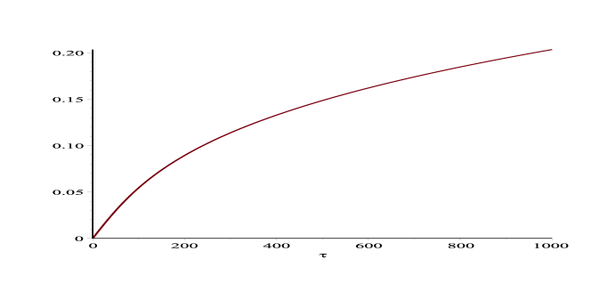
Figure 1: Numerical plot of $u(\tau)$ for $a=-8$ and $b=1/100$.

It is know [1] that $u(\tau)$ is, in fact, oscillating about the parabola in Figure 1; however, this oscillatory structure is too fine to be observed for $a<-1$.

Figure 2: Plot of $\int_{0}^{\tau}\left(2a/{\tilde{\tau}}+b/u(\tilde{\tau})\right)d\tilde{\tau}$ for $a=-8$ and $b=1/100$. The upper line is the asymptotics and the lower line is the numerical plot of the integral.

For the calculation of asymptotics, via Equation (2), in Figure 2 it is important to note that $\mathrm{Arg}\left(\Gamma(1-8i)\right)=\arg\left(\Gamma(1-8i)\right)-2\pi$.

According to Equation (13), the plots in Figures 2 and 5 for $\mathrm{Re}\int_{0}^{\tau}\left(f(\tilde{\tau})/{\tilde{\tau}}\right)d\tilde{\tau}$ coincide modulo the numeric factor $b/8$.

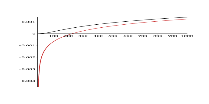
Figure 3: Plot of $\mathrm{Im}\int_{0}^{\tau}\left(f(\tilde{\tau})/{\tilde{\tau}}\right)d\tilde{\tau}$ for $a=-8$ and $b=1/100$. The upper line is the numerical plot of the integral and the lower line is the plot of its asymptotics (14).

The correction term (15) is not observable in Figure 3: this is the general situation for all values $a<-1$; it is obviously related with the analogous situation for $u(\tau)$.

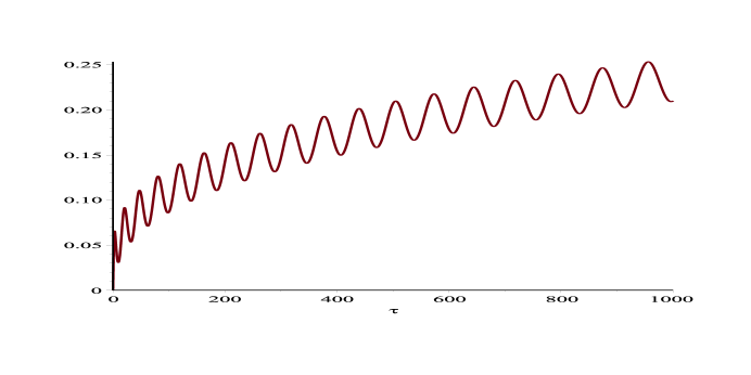
Figure 4: Numerical plot of $u(\tau)$ for $a=-1/8$ and $b=1/100$.

For $-1<a<0$, oscillations of the solution (which are “hidden” for smaller values of $a$) are clearly seen.

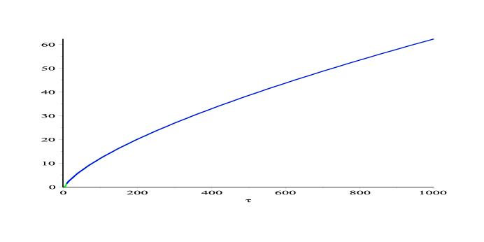
Figure 5: Plot of $\int_{0}^{\tau}\left(2a/{\tilde{\tau}}+b/u(\tilde{\tau})\right)d\tilde{\tau}$ for $a=-1/8$ and $b=1/100$. The asymptotic and numerical solutions practically coincide for $\tau>5$.

Oscillations that are seen in Figure 4 are not observable in Figure 5, and, consequently, for $\mathrm{Re}\int_{0}^{\tau}\left(f(\tilde{\tau})/{\tilde{\tau}}\right)d\tilde{\tau}$.

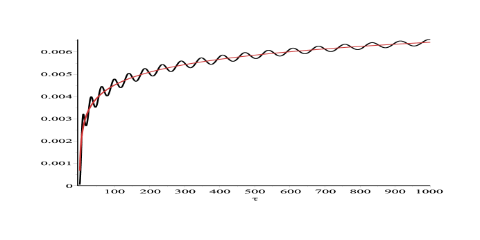
Figure 6: Plot of $\mathrm{Im}\int_{0}^{\tau}\left(f(\tilde{\tau})/{\tilde{\tau}}\right)d\tilde{\tau}$ for $a=-1/8$ and $b=1/100$. One sees oscillation of the numerical solution about the asymptotic line (14) without the correction term (15).

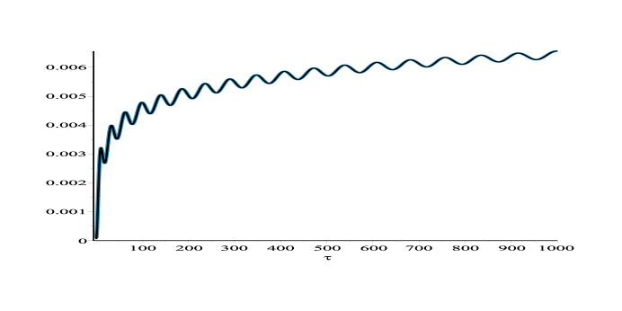
Figure 7: Plot of $\mathrm{Im}\int_{0}^{\tau}\left(f(\tilde{\tau})/{\tilde{\tau}}\right)d\tilde{\tau}$ for $a=-1/8$ and $b=1/100$. One notes that the numerical solution practically coincides with the asymptotic solution with the correction term (15).

Figures 6 and 7 illustrate, for $-1<a<0$, the importance of the correction term (15) for $\mathrm{Im}\int_{0}^{\tau}\left(f(\tilde{\tau})/{\tilde{\tau}}\right)d\tilde{\tau}$.

Note that the value of the parameter $b>0$ is not important for observing the oscillations; for larger values of $b$, the oscillations become faster. The value $b=1/100$ is chosen only for the purpose of obtaining clearer figures.

References

- [1] A. V. Kitaev and A. H. Vartanian, Connection formulae for asymptotics of solutions of the degenerate third Painlevé equation: I, Inverse Problems 20, no. 4, 1165–1206 (2004).
- [2] A. V. Kitaev and A. Vartanian, Connection formulae for asymptotics of solutions of the degenerate third Painlevé equation: II, Inverse Problems 26, no. 10, 105010 (2010).
- [3] K. Okamoto, On the -function of the Painlevé equations, Physica 2D, 525-535 (1981).
- [4] M. Jimbo and T. Miwa, Monodromy preserving deformation of linear ordinary differential equations with rational coefficients II, Physica 2D, 407–448 (1981).
- [5] C. M. Cosgrove and G. Scofus, Painlevé Classification of a Class of Differential Equations of the Second Order and Second Degree, Stud. Appl. Math. 88, no. 1, 25–87 (1993).
- [6] F. Bureau, Équations différentielles du second ordre en Y et du second degré en Ÿ dont l’intégrale générale est à points critiques fixes, Ann. Mat. Pura Appl. (4) 91, 163-281 (1972).
- [7] A. V. Kitaev, Meromorphic Solution of the Degenerate Third Painlevé Equation Vanishing at the Origin, https://arxiv.org/abs/1809.00122.
- [8] J. Baik, R. Buckingham, J. DiFranco, and A. Its, Total integrals of global solutions to Painlevé II, Nonlinearity 22, no. 5, 1021–1061 (2009).
- [9] A. Erdélyi, W. Magnus, F. Oberhettinger, F. G. Tricomi, Higher Transcendental Functions, Vol. 1, McGraw-Hill Book Company, Inc., New York-Toronto-London (1953) (based, in part, on notes left by Harry Bateman).