G11.92$-$0.61 MM 1: A FRAGMENTED KEPLERIAN DISK SURROUNDING A PROTO-O STAR

Abstract

We present high resolution ($\sim$300 au) Atacama Large Millimeter/submillimeter Array (ALMA) observations of the massive young stellar object G11.92$-$0.61 MM 1. We resolve the immediate circumstellar environment of MM 1 in 1.3 mm continuum emission and CH₃CN emission for the first time. The object divides into two main sources — MM 1a, which is the source of a bipolar molecular outflow, and MM 1b, located $0\farcs 57$ (1920 au) to the South-East. The main component of MM 1a is an elongated continuum structure, perpendicular to the bipolar outflow, with a size of $0\farcs 141\times 0\farcs 050$ ($480\times 170$ au). The gas kinematics toward MM 1a probed via CH₃CN trace a variety of scales. The lower energy $J=12$–11 $K=3$ line traces extended, rotating gas within the outflow cavity, while the $v$8=1 line shows a clearly-resolved Keplerian rotation signature. Analysis of the gas kinematics and dust emission shows that the total enclosed mass in MM 1a is $40\pm 5$ M_⊙ (where between 2.2–5.8 M_⊙ is attributed to the disk), while MM 1b is $<0.6$ M_⊙. The extreme mass ratio and orbital properties of MM 1a and MM 1b suggest that MM 1b is one of the first observed examples of the formation of a binary star via disk fragmentation around a massive young (proto)star.

1 Introduction

The formation mechanisms of massive young stellar objects (MYSOs, $M_{\star}>8\,M_{\odot}$) are poorly understood due to their large distances and extreme embedded nature. Models have suggested that channelling material through a circumstellar accretion disk can overcome the powerful feedback from the central protostar (Krumholz et al., 2009; Kuiper et al., 2011; Rosen et al., 2016). Such models predict that these disks possess significant sub-structure, including large scale spiral arms and bound fragments (Klassen et al., 2016; Harries et al., 2017; Meyer et al., 2018). Observationally, however, it is not clear whether Keplerian circumstellar disks surround MYSOs of all masses and evolutionary stages (see Beltrán & de Wit, 2016, for a review), though convincing candidates are beginning to emerge (Johnston et al., 2015; Ilee et al., 2016). In many cases, complex velocity structures, high continuum optical depths, and potential multiplicity (e.g. Maud et al., 2017; Cesaroni et al., 2017; Beuther et al., 2018; Csengeri et al., 2018; Ahmadi et al., 2018) make comprehensive characterisation of the physical properties of these disks challenging.

Such characterisation is important in order to connect the processes of massive star formation with the population of massive O- and B-type stars observed in the field. High-resolution radial velocity surveys have found that $>80$ per cent of OB stars are found in close binary systems (Chini et al., 2012). Do these high-mass multiple stellar systems form via the large-scale fragmentation of turbulent cloud cores (e.g. Fisher, 2004), or via smaller-scale fragmentation of a massive protostellar disk (e.g. Adams et al., 1989)? Answering such a question requires high angular resolution observations of individual, deeply-embedded massive protostellar systems that are still in the process of formation.

G11.92–0.61 MM 1 (hereafter MM 1) was identified during studies of GLIMPSE Extended Green Objects (EGOs; Cyganowski et al., 2008), and is located in an infrared dark cloud (IRDC) $\sim$1′ SW of the more evolved massive star-forming region IRAS 18110–1854. The total luminosity of G11.92$-$0.61 is $\sim$10⁴$L_{\odot}$(Cyganowski et al., 2011; Moscadelli et al., 2016), and its distance is 3.37${}^{+0.39}_{-0.32}$ kpc (based on maser parallaxes; Sato et al., 2014). MM 1 drives a single, dominant bipolar molecular outflow traced by well-collimated, high-velocity ¹²CO(2–1) and HCO⁺(1–0) emission (Cyganowski et al., 2011), and is coincident with a 6.7 GHz Class II CH₃OH and strong H₂O masers (Hofner & Churchwell, 1996; Cyganowski et al., 2009; Breen & Ellingsen, 2011; Sato et al., 2014; Moscadelli et al., 2016). All of these characteristics suggest the presence of a massive (proto)star.

In Ilee et al. (2016), we analysed the properties of the centimeter and millimeter emission from MM 1. Our 1.3 mm Submillimeter Array (SMA) observations (resolution $\sim$ $0\farcs 46$, 1550 au) showed consistent velocity gradients across multiple hot-core-tracing molecules oriented perpendicular to the bipolar molecular outflow. The kinematics of these lines suggested an infalling Keplerian disk with a radius of 1200 au, surrounding an enclosed mass of $\sim$30–60 M_⊙, of which 2–3 M_⊙ could be attributed to the disk. Such a massive, extended Keplerian disk brings into question its stability against gravitational fragmentation. In Forgan et al. (2016), we performed a detailed analysis of MM 1 (and other systems) utilising semi-analytic models of self-gravitating disks. For the properties determined from our SMA observations, the disk around MM 1 satisfies all conditions for fragmentation, with the models predicting fragment masses of $\sim$0.4 M_⊙ for disk radii $\sim$1200 au when accretion rates are $\gtrsim 10^{-4}$ M_⊙ yr^-1.

In this Letter, we report high spatial and spectral resolution line and continuum ALMA observations of G11.92$-$0.61 MM 1 that were designed to further characterise the circumstellar environment of this massive young stellar object, and search for evidence of disk fragmentation.

2 Observations

Our ALMA observations were taken on 2017 Aug 07 (project ID 2016.1.01147.S, PI: J. D. Ilee) in configuration C40-7 with 46 antennas. The projected baselines ranged from $\sim$15–2800 k$\lambda$. We observed in Band 6 (230 GHz, 1.3 mm) with four SPWs (220.26–220.73, 221.00–221.94, 235.28–236.22 and 238.35–239.29 GHz) for an on-source time of 93 mins. Imaging with Briggs weighting with a robust parameter of 0 yielded a synthesised beamsize of $0\farcs 106\times 0\farcs 079$ ($360\times 270$ au), PA$=-63.7^{\circ}$ East of North, and a largest recoverable scale of $0\farcs 58$ (1955 au). Calibration, imaging and analysis were performed with CASA version 5.1.1 (McMullin et al., 2007). The continuum data were self-calibrated iteratively, with phase and amplitude solution times of 6 and 54 seconds, respectively, with a resulting S/N of 569 (an improvement factor of 1.4). The continuum self-calibration solutions were also applied to the line data. Continuum subtraction was performed following the method of Brogan et al. (2018), resulting in a continuum bandwidth of 0.38 GHz and sensitivity of 0.05 mJy beam^-1. The line data were re-sampled to a common velocity resolution of 0.7 km s^-1 to improve signal-to-noise, achieving a typical per-channel sensitivity of 1.2 mJy beam^-1.

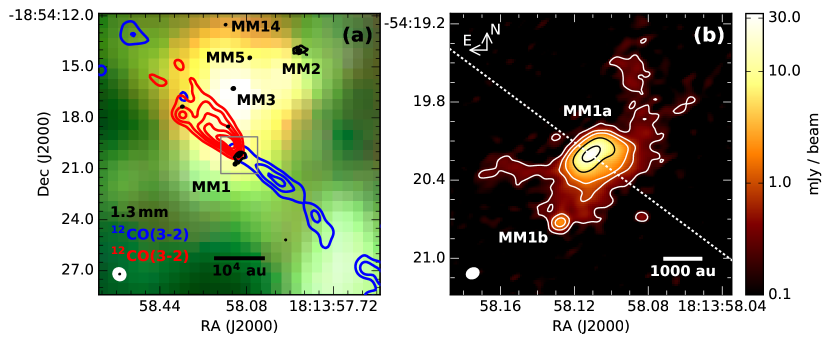
Figure 1: (a): G11.92$-$0.61: ALMA 1.3 mm continuum emission (black contours) and SMA blue/redshifted ¹²CO(3–2) integrated intensity (blue: $-16$–$20$ km s^-1, red: $50$–$74$ km s^-1) overlaid on a three-color Spitzer image (RGB: 8.0, 4.5, 3.6 $\mu$m). Levels: 1.3 mm: (5,150)$\sigma$, $\sigma=0.05$ mJy beam^-1; ¹²CO: 0.8 Jy beam^-1 km s^-1 $\times$(5,10,15) (blue), $\times$(5,10,15,20,25) (red). (b): Zoom view of the ALMA 1.3 mm continuum emission towards MM 1 (colorscale & contours; the grey box in (a) shows the FOV of (b)). The dotted white line shows the position angle of the ¹²CO outflow ($53\arcdeg$). Levels: (5,15,30,100,400)$\sigma$, $\sigma=0.05$ mJy beam^-1. Beams are shown at lower left.

Table 1: Fitted properties: 1.3 mm continuum

Source	Fitted Position (J2000)		Integ. Flux Density	Peak Intensity	Tb	FWHM of deconvolved Gaussian model
	$\alpha~{}({{}^{\rm h}~{}^{\rm m}~{}^{\rm s}}$)	$\delta~{}(^{\circ}~{}\arcmin~{}\arcsec)$	(mJy)	(mJy beam-1)	(K)	(${}^{\prime\prime}\times^{\prime\prime}$ [P.A.($\arcdeg$)])
MM 1a
xx$ii$$(i)$ – Main disk	18:13:58.111	$-$18:54:20.205	53.2 (0.6)	26.8 (0.2)	93	$0.141\times 0.050$ ($0.002$) [+129.4 (0.1)]
xx$i$$(ii)$ – SW excess	18:13:58.108	$-$18:54:20.266	44.1 (2.0)	3.5 (0.2)	11	$0.39\times 0.24$ ($0.02$) [+119 (4)]
xx$(iii)$ – W excess	18:13:58.104	$-$18:54:20.140	10.2 (0.7)	4.4 (0.2)	62	$0.17\times 0.02$ ($0.02$) [+62 (3)]
$(iv)$ – Free-free	18:13:58.111	$-$18:54:20.185	4.0	4.0	…	…
MM 1b	18:13:58.128	$-$18:54:20.721	2.5 (0.2)	2.1 (0.1)	6	$0.069\times 0.016$ ($0.02$) [+35 (43)]

3 Results

3.1 1.3 mm continuum emission

Figure 1 shows two views of our new ALMA observations of G11.92$-$0.61. Fig. 1a shows a larger-scale view ($\sim 16\arcsec\times 16\arcsec\sim$0.27 pc²), including the large-scale, well-collimated bipolar outflow from MM 1 (traced by ¹²CO(3–2) observed with the SMA; Cyganowski et al., 2011). Fig. 1b shows a zoom view of the 1.3 mm continuum emission toward MM 1, revealing two main sources. The dominant source, MM 1a, is the source of the bipolar outflow (marked with a dotted line). Situated 0$\farcs$57 (1920 au) to the South-East of MM 1a is a weaker source, MM 1b, which is connected to MM 1a via smooth background emission at a level of $\sim$0.5 mJy beam^-1. Fitting in the image plane of both the compact and elongated continuum emission within $\sim$1000 au of MM 1a requires four individual 2D Gaussian components (see Table 1). Peak residuals from the combination of these fits lie at the 2$\sigma$ level (0.1 mJy beam^-1). Beyond the central $\sim$1000 au, we also report a fit to the continuum toward MM 1b.

3.2 CH₃CN emission

Figure 2a presents integrated intensity and intensity-weighted velocity maps of the CH₃CN $v$8=1 $K=(1,-1)$ transition (221.625 GHz, $E_{\rm up}=588$ K). The high excitation energy of this transition allows us to trace hot, dense gas within the inner 1000 au of the circumstellar material. The velocity field of the $v$8=1 transition exhibits rotation perpendicular to the outflow axis. Figure 2b shows a position-velocity (PV) diagram for a slice along the major axis of the emission (length = 2$\farcs$0, PA = 129.4^∘, centered on the continuum peak). Both the velocity field and PV diagram are consistent with expectations for a Keplerian disk – high central velocities showing an approximately square-root drop-off with distance.

Figures 3a & 3b present integrated intensity, intensity-weighted velocity and intensity-weighted velocity dispersion maps for the CH₃CN $J=12$–11 $K=3$ transition (220.709 GHz, $E_{\rm up}=93$ K). In contrast to the $v8$=1 transition, the $K=3$ emission traces gas with a lower excitation energy and a larger spatial extent around MM 1. The integrated intensity map (Fig. 3a) exhibits a rectangular morphology, aligned with the position angle of the bipolar outflow, which suggests the emission is tracing material in the outflow cavity. Measured opening angles from the corners of this shape are 88^∘ and 55^∘ for the North-East and South-West cavities, respectively. The velocity field reveals a large-scale rotation pattern that is broadly consistent with the $v$8=1 transition, but with significant local deviations. The velocity dispersion map (Fig. 3b) displays a trend of increasing velocity dispersion closer to the continuum peak of MM 1a, with additional localised increases along the outflow axis. In particular, the area NE of MM1a shows a high dispersion, of 6-7 km s^-1, which is not mirrored to the SW. At the location of MM 1b, deviations are observed in the integrated intensity, velocity and velocity dispersion, showing it is an outlier when compared to the surrounding material.

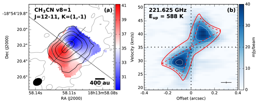
Figure 2: (a): Integrated intensity (black contours) and intensity-weighted velocity (colorscale) of the vibrationally-excited CH₃CN $J=12$–11, $K=($1,$-$1) line ($E_{\rm up}=588$ K) toward MM 1a, overlaid with the 1.3 mm continuum contours from Figure 1 (in grey). A white star marks the continuum peak, and the position angle of the ¹²CO outflow ($53^{\circ}$) is shown with a dotted line. Integrated intensity levels: (5,15,30,60)$\sigma$, $\sigma=6.1$ mJy beam^-1 km s^-1. The beam is shown in the lower left. (b): Position-velocity (PV) diagram taken along the grey line in (a). White contours mark levels of 10, 20, 30 and 40 mJy beam^-1. Dotted black lines denote zero offset and the $v_{\rm lsr}$. Overlaid in red are models of a thin Keplerian disk ($R_{\rm i}=270$, $R_{\rm o}=850$ au) surrounding an enclosed mass M_enc=40 M_⊙ viewed at an inclination of 70^∘. The solid and dashed red lines show models with and without infalling motions at 40% of the free-fall velocities, respectively. The spatial and spectral resolutions are shown with a black cross.

4 Discussion

4.1 Mass estimates from the gas kinematics

Using our observations of the $v$8=1 line, we can assess the enclosed mass, $M_{\rm enc}$, within such a rotating Keplerian disk. Following Cesaroni et al. (2011), the expected shape of the region in PV space from which emission will originate can be expressed as

$$V=\sqrt{GM_{\rm enc}}\frac{x}{R^{\frac{3}{2}}}+\beta\sqrt{2GM_{\rm enc}}\frac{z}{R^{\frac{3}{2}}},$$ (1)

where the first term is the contribution from the Keplerian disk, and the second the contribution due to free fall. $V$ is the velocity component along the line-of-sight, $M_{\rm enc}$ is the enclosed mass, $x$ and $z$ are the co-ordinates along the disk plane and line-of-sight, respectively, $R=\sqrt{x^{2}+z^{2}}$ is the radial distance from the center of the disk (where $R_{\rm i}<R<R_{\rm o}$), and $\beta$ is a fractional factor for the contribution of the free-fall velocity.

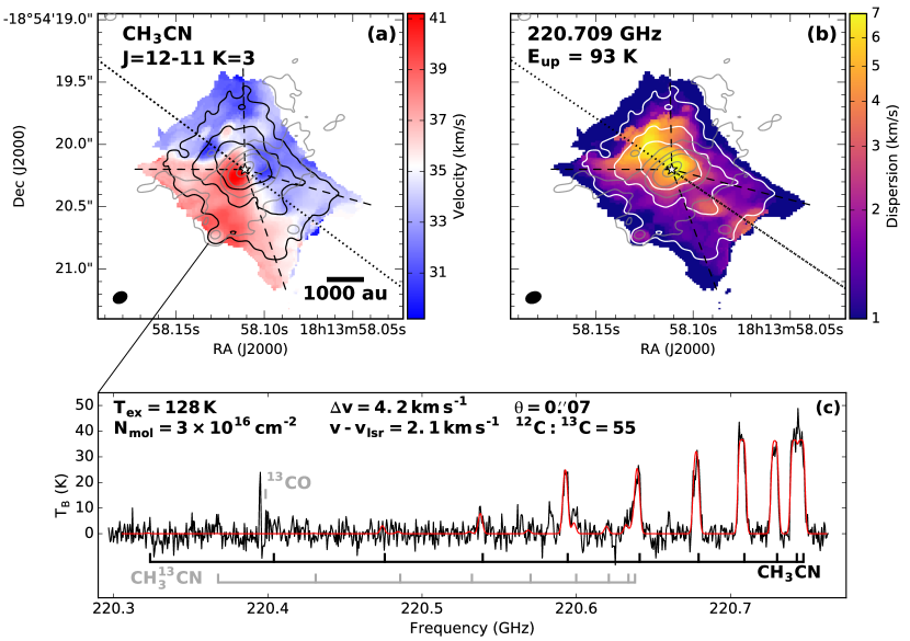
Figure 3: MM1 1.3 mm continuum contours (from Figure 1, in grey) overlaid on (a): Integrated intensity (black contours) and intensity-weighted velocity (colorscale) of the CH₃CN $J=12$–11 $K=3$ line ($E_{\rm up}=93$ K). The black dotted line shows the position angle of the CO outflow, and black dashed lines the measured opening angles (NE: 88^∘, SW: 55^∘). Integrated intensity levels: (5,15,30)$\sigma$, $\sigma=11.5$ mJy beam^-1 km s^-1 (b): Integrated intensity (white contours) and intensity-weighted velocity dispersion (colorscale) of the $K=3$ line. (c): The CASSIS fit (red) to the CH₃CN and CH${}_{3}^{13}$CN $J=12$–11 emission (black) at the MM 1b continuum peak. Best fitting parameters are labelled, and the frequencies of individual transitions are marked.

Our spatially resolved observations of the 1.3 mm continuum emission (Section 3.1) allow us to break the degeneracy between an unknown disk inclination and enclosed mass. If we assume that component ($i$) represents a flat, inclined disk, then its fitted size ($0\farcs 141\times 0\farcs 050$, Table 1) corresponds to an inclination $i\sim 70$^∘ to the line of sight (where 0^∘ corresponds to a face-on disk). Since simulations of similar disks have been shown to possess moderate aspect ratios ($H/R\lesssim 0.15$, Harries et al. 2017), we ascribe a conservative uncertainty of $\pm 10$^∘ to this inclination to account for projection effects. The inner extent of the emission is unknown, and direct measurements may be confused by significant continuum opacity (see Jankovic et al., 2018, their Section 4.3) or chemical/radiative processes depleting the gas-phase abundance of CH₃CN. Thus we fix the inner radius to the beamsize, $R_{\rm in}=270$ au. We then perform a by-eye fit to the offset and velocity by altering the outer radius of the emission (in steps of half the geometric mean of the beamsize, $0\farcs 045\sim$150 au) and the enclosed mass (in steps of 5 M_⊙). Our exploration of this parameter space yields best fitting values of $R_{\rm out}=850$ au and $M_{\rm enc}=40$ M_⊙ (Figure 2b, dashed red line). A purely Keplerian model does not reproduce all of the emission in PV space; to do so, our final model includes a uniform in-falling component at 40 per cent of the free-fall velocity (Figure 2b, solid red line). We note that this process is unable to account for beam convolution effects, and similarly best fitting models can be obtained with $M_{\rm enc}=40\pm 5$ M_⊙ for $i=70\mp 10$^∘.

4.2 Physical conditions toward MM 1b

In order to determine the physical properties of the gas toward MM 1b, we model the CH₃CN and CH${}_{3}^{13}$CN emission line ladders. Figure 3c shows the spectrum around the $J=12-11$ ladder extracted at the continuum peak of MM 1b. We utilise the CASSIS local thermodynamic equilibrium (LTE) radiative transfer package. Six free parameters were explored — CH₃CN column density: $10^{16}<N_{\rm mol}<10^{19}$ cm^-2; excitation temperature: $10<T_{\mathrm{ex}}<450$ K; line width: $1<\Delta v<10$ km s^-1; size: $0.02\arcsec<\theta<0.2\arcsec$; velocity: $-5<v-v_{\rm lsr}<5$ km s^-1; isotopic ratio: $55<\,{\mathrm{{}^{12}C}:\mathrm{{}^{13}C}}<85$. Fitting was performed using Markov-Chain Monte Carlo minimisation with 10⁴ iterations, a cut-off parameter of 5000, and an acceptance rate of 0.5 (for details see Ilee et al., 2016). The resulting best fit is shown by the red line in Figure 3c with parameters $N_{\rm mol}=3\times 10^{16}$ cm^-2; $T_{\mathrm{ex}}=128$ K; $\Delta v=4.2$ km s^-1; $v-v_{\rm lsr}=2.1\,$km s^-1; $\theta=0\farcs 07$ and ${{}^{12}\mathrm{C}:^{13}\mathrm{C}}=55$.

4.3 Mass estimates from the dust emission

Modelling of the centimeter to submillimeter wavelength SED of MM 1 confirms that the observed 1.3 mm flux density is dominated by thermal dust emission (99.5 per cent, Ilee et al. 2016). We can therefore estimate gas masses from the 1.3 mm integrated flux densities for the various components of MM 1. We utilise a simple model of isothermal dust emission, corrected for dust opacity (Cyganowski et al., 2011, Equation 3), assuming a gas-to-dust mass ratio of 100 and a dust opacity of $\kappa_{\rm 1.3\,mm}=1.1$ cm² g^-1 (for grains with thin ice mantles and coagulation at $10^{8}$ cm^-3; Ossenkopf & Henning 1994). For each component, we utilise two temperature estimates to bracket the plausible range for the circumstellar material. In MM 1a, for the main disk we take 150–230 K based on the modelling of the CH₃CN $J=12$–11 emission toward MM 1 in Ilee et al. (2016). For the SW and W excesses, we adopt 65 – 150 K based on their increased radial distance from the central source. In MM 1b, we take 20 – 128 K, where the latter is based on the fit to the CH₃CN $J=12$–11 ladder in Section 4.2. Under these assumptions, the mass of the main disk ranges from 0.9 – 1.7 M_⊙, the total mass of continuum components $i$–$iii$ ranges from 2.2 – 5.8 M_⊙, and the mass of MM 1b ranges from 0.06 – 0.6 M_⊙.

Under the assumption that the gas kinematics around MM 1b are also dominated by a Keplerian disk, we can obtain an estimate for its enclosed mass. Using the fitted size of the 1.3 mm continuum emission (0$\farcs$069, 233 au, Table 1) and the linewidth from fits to the CH₃CN ladder (4.2 km s^-1, Fig. 3c), $M_{\rm enc}=R(V/\sin i)^{2}/G=116\,{\rm au}(2.1\,{\rm km}\,{\rm s}^{-1}/\sin i)^{2}/G=0.57/\sin^{2}i\,\mathrm{M}_{\odot}$ (following Hunter et al., 2014). Such a dynamical mass would include any contribution from a central object in MM 1b in addition to the mass calculated from the millimeter continuum. Therefore, the inclination of a putative disk around MM 1b must be $\lesssim 65$^∘ if the central mass is $\gtrsim 0.1\,\mathrm{M}_{\odot}$.

4.4 The MM 1a & b system:
a result of disk fragmentation?

The combination of dynamical and continuum masses derived above allows us to place a lower limit on the mass of the central object in the MM 1 system. We estimate the minimum mass of the central object in MM 1a as $(40\pm 5)-5.8\sim 34\pm 5$ M_⊙, placing it comfortably within the O spectral class (Martins et al., 2005). In contrast, the mass derived for MM 1b ($<$0.6 M_⊙) corresponds to an M-dwarf or later spectral type. The radial velocity of MM 1b with respect to MM 1a (2.1km s^-1, Section 4.2) shows it is orbiting in the same sense as the Keplerian disk. MM 1b appears to be stable against disruption in such an orbital configuration, since the fitted size of the major axis of MM 1b (0$\farcs$069, 233 au) is comfortably within its Hill sphere:

$$r_{\rm H}\sim 1920\,{\rm au}\sqrt[3]{\frac{0.6\,{\rm M}_{\odot}}{3\times 40\,{\rm M}_{\odot}}}\sim 330\,{\rm au}.$$ (2)

The expected orbital period of MM 1b, $P=1.3\times 10^{4}$ yrs, is comparable to the dynamical timescale of the bipolar outflow driven by MM 1a ($\lesssim 10^{4}$ yrs, Cyganowski et al. 2011). In addition, the opening angles of the outflow cavity (88^∘ and 55^∘, Section 3.2) are comparable to those in the simulations of Kuiper et al. (2016) at the onset of radiation pressure feedback, $<5\times 10^{5}$ yrs. All of these observed properties point toward a young age for the MM 1 system.

Our detection of MM 1b raises the question: what is the origin of a system of objects with such an unequal mass ratio ($q\sim 0.015$)? Fragmentation of turbulent cloud cores has been shown to produce close ($\lesssim$10 au) binary systems, but due to dynamical interactions and accretion, these binaries do not possess extreme mass ratios ($q\gtrsim 0.3$, Bate et al. 2002). Fragmentation of an extended circumstellar disk is an alternative route to produce extreme mass ratio systems with larger separations (Clarke, 2009), which are observed on the main sequence (Moe & Di Stefano, 2017). In striking similarity to our observed properties for MM 1a and 1b, Kratter & Matzner (2006) find that O stars can be expected to be surrounded by M5–G5 companions. In addition, our measured mass for MM 1b agrees well with predictions for masses of fragments formed via gravitational disk fragmentation at similar radii (e.g. 0.4 M_⊙ at 1200 au; Forgan et al. 2016). The combined evidence thus strongly suggests that MM 1b has formed via the fragmentation of an extended circumstellar disk around MM 1a.

Finally, the fact that the central protostar powering MM1a is significantly underluminous compared to a main sequence star of equal mass means that its energy output is currently dominated by accretion. Indeed, the relative length of this evolutionary state prior to reaching the ZAMS may determine the likelihood of formation of companions like MM 1b. This speculation can be tested by identifying more examples of disk fragmentation around massive protostars.

5 Conclusions

In this Letter, we have resolved the immediate circumstellar environment of the high-mass (proto)star G11.92–0.61 MM 1 for the first time. Our observations show that MM 1 separates into two main sources – MM 1a (the source of the bipolar outflow) and MM 1b. The main component of MM 1a is an elongated millimeter-continuum structure, approximately perpendicular to the bipolar outflow. CH₃CN $J=12-11$ $K=3$ emission traces a rotating outflow cavity, while the $v$8=1 transition exhibits a kinematic signature consistent with the rotation of a Keplerian disk. We find an enclosed mass of $40\pm 5$ M_⊙, of which 2.2–5.8 M_⊙ can be attributed to the disk, while the mass of MM 1b is $<0.6$ M_⊙. Based on the orbital properties and the extreme mass ratio of these objects, we suggest that MM 1b is one of the first observed examples of disk fragmentation around a high mass (proto)star.

Our results demonstrate that G11.92$-$0.61 MM 1 is one of the clearest examples of a forming proto-O star discovered to date, and show its potential as a laboratory to test theories of massive (binary) star formation.

References

- Adams et al. (1989) Adams, F. C., Ruden, S. P., & Shu, F. H. 1989, ApJ, 347, 959, doi: 10.1086/168187
- Ahmadi et al. (2018) Ahmadi, A., Beuther, H., Mottram, J. C., et al. 2018, ArXiv e-prints. https://arxiv.org/abs/1808.00472
- Astropy Collaboration et al. (2013) Astropy Collaboration, Robitaille, T. P., Tollerud, E. J., et al. 2013, A&A, 558, A33, doi: 10.1051/0004-6361/201322068
- Bate et al. (2002) Bate, M. R., Bonnell, I. A., & Bromm, V. 2002, MNRAS, 336, 705, doi: 10.1046/j.1365-8711.2002.05775.x
- Beltrán & de Wit (2016) Beltrán, M. T., & de Wit, W. J. 2016, A&A Rev., 24, 6, doi: 10.1007/s00159-015-0089-z
- Beuther et al. (2018) Beuther, H., Mottram, J. C., Ahmadi, A., et al. 2018, ArXiv e-prints. https://arxiv.org/abs/1805.01191
- Breen & Ellingsen (2011) Breen, S. L., & Ellingsen, S. P. 2011, MNRAS, 416, 178, doi: 10.1111/j.1365-2966.2011.19020.x
- Brogan et al. (2018) Brogan, C. L., Hunter, T. R., Cyganowski, C. J., et al. 2018, ArXiv e-prints. https://arxiv.org/abs/1809.04178
- Cesaroni et al. (2011) Cesaroni, R., Beltrán, M. T., Zhang, Q., Beuther, H., & Fallscheer, C. 2011, A&A, 533, A73, doi: 10.1051/0004-6361/201117206
- Cesaroni et al. (2017) Cesaroni, R., Sánchez-Monge, Á., Beltrán, M. T., et al. 2017, A&A, 602, A59, doi: 10.1051/0004-6361/201630184
- Chini et al. (2012) Chini, R., Hoffmeister, V. H., Nasseri, A., Stahl, O., & Zinnecker, H. 2012, MNRAS, 424, 1925, doi: 10.1111/j.1365-2966.2012.21317.x
- Clarke (2009) Clarke, C. J. 2009, MNRAS, 396, 1066, doi: 10.1111/j.1365-2966.2009.14774.x
- Csengeri et al. (2018) Csengeri, T., Bontemps, S., Wyrowski, F., et al. 2018, ArXiv e-prints. https://arxiv.org/abs/1804.06482
- Cyganowski et al. (2009) Cyganowski, C. J., Brogan, C. L., Hunter, T. R., & Churchwell, E. 2009, ApJ, 702, 1615, doi: 10.1088/0004-637X/702/2/1615
- Cyganowski et al. (2011) Cyganowski, C. J., Brogan, C. L., Hunter, T. R., Churchwell, E., & Zhang, Q. 2011, ApJ, 729, 124, doi: 10.1088/0004-637X/729/2/124
- Cyganowski et al. (2008) Cyganowski, C. J., Whitney, B. A., Holden, E., et al. 2008, AJ, 136, 2391, doi: 10.1088/0004-6256/136/6/2391
- Fisher (2004) Fisher, R. T. 2004, ApJ, 600, 769, doi: 10.1086/380111
- Forgan et al. (2016) Forgan, D. H., Ilee, J. D., Cyganowski, C. J., Brogan, C. L., & Hunter, T. R. 2016, MNRAS, 463, 957, doi: 10.1093/mnras/stw1917
- Harries et al. (2017) Harries, T. J., Douglas, T. A., & Ali, A. 2017, MNRAS, 471, 4111, doi: 10.1093/mnras/stx1490
- Hofner & Churchwell (1996) Hofner, P., & Churchwell, E. 1996, A&AS, 120, 283
- Hunter et al. (2014) Hunter, T. R., Brogan, C. L., Cyganowski, C. J., & Young, K. H. 2014, ApJ, 788, 187, doi: 10.1088/0004-637X/788/2/187
- Ilee et al. (2016) Ilee, J. D., Cyganowski, C. J., Nazari, P., et al. 2016, MNRAS, 462, 4386, doi: 10.1093/mnras/stw1912
- Jankovic et al. (2018) Jankovic, M. R., Haworth, T. J., Ilee, J. D., et al. 2018, ArXiv e-prints. https://arxiv.org/abs/1810.11398
- Johnston et al. (2015) Johnston, K. G., Robitaille, T. P., Beuther, H., et al. 2015, ApJ, 813, L19, doi: 10.1088/2041-8205/813/1/L19
- Klassen et al. (2016) Klassen, M., Pudritz, R., Kuiper, R., Peters, T., & Banerjee, R. 2016, ArXiv e-prints. https://arxiv.org/abs/1603.07345
- Kratter & Matzner (2006) Kratter, K. M., & Matzner, C. D. 2006, MNRAS, 373, 1563, doi: 10.1111/j.1365-2966.2006.11103.x
- Krumholz et al. (2009) Krumholz, M. R., Klein, R. I., McKee, C. F., Offner, S. S. R., & Cunningham, A. J. 2009, Science, 323, 754, doi: 10.1126/science.1165857
- Kuiper et al. (2011) Kuiper, R., Klahr, H., Beuther, H., & Henning, T. 2011, ApJ, 732, 20, doi: 10.1088/0004-637X/732/1/20
- Kuiper et al. (2016) Kuiper, R., Turner, N. J., & Yorke, H. W. 2016, ApJ, 832, 40, doi: 10.3847/0004-637X/832/1/40
- Martins et al. (2005) Martins, F., Schaerer, D., & Hillier, D. J. 2005, A&A, 436, 1049, doi: 10.1051/0004-6361:20042386
- Maud et al. (2017) Maud, L. T., Hoare, M. G., Galván-Madrid, R., et al. 2017, MNRAS, 467, L120, doi: 10.1093/mnrasl/slx010
- McMullin et al. (2007) McMullin, J. P., Waters, B., Schiebel, D., Young, W., & Golap, K. 2007, in Astronomical Society of the Pacific Conference Series, Vol. 376, Astronomical Data Analysis Software and Systems XVI, ed. R. A. Shaw, F. Hill, & D. J. Bell, 127
- Meyer et al. (2018) Meyer, D. M.-A., Kuiper, R., Kley, W., Johnston, K. G., & Vorobyov, E. 2018, MNRAS, 473, 3615, doi: 10.1093/mnras/stx2551
- Moe & Di Stefano (2017) Moe, M., & Di Stefano, R. 2017, ApJS, 230, 15, doi: 10.3847/1538-4365/aa6fb6
- Moscadelli et al. (2016) Moscadelli, L., Sánchez-Monge, Á., Goddi, C., et al. 2016, A&A, 585, A71, doi: 10.1051/0004-6361/201526238
- Ossenkopf & Henning (1994) Ossenkopf, V., & Henning, T. 1994, A&A, 291, 943
- Robitaille & Bressert (2012) Robitaille, T., & Bressert, E. 2012, APLpy: Astronomical Plotting Library in Python, Astrophysics Source Code Library. http://ascl.net/1208.017
- Rosen et al. (2016) Rosen, A. L., Krumholz, M. R., McKee, C. F., & Klein, R. I. 2016, MNRAS, 463, 2553, doi: 10.1093/mnras/stw2153
- Sato et al. (2014) Sato, M., Wu, Y. W., Immer, K., et al. 2014, ApJ, 793, 72, doi: 10.1088/0004-637X/793/2/72