Long term measurements from the Mátra Gravitational and Geophysical Laboratory

Abstract.

Summary of the long term data taking, related to one of the proposed next generation ground-based gravitational detector’s location is presented here. Results of seismic and infrasound noise, electromagnetic attenuation and cosmic muon radiation measurements are reported in the underground Matra Gravitational and Geophysical Laboratory near Gyöngyösoroszi, Hungary. The collected seismic data of more than two years is evaluated from the point of view of the Einstein Telescope, a proposed third generation underground gravitational wave observatory. Applying our results for the site selection will significantly improve the signal to nose ratio of the multi-messenger astrophysics era, especially at the low frequency regime.

1. Introduction

Preparation for the next generation ground-based gravitational detectors requires careful pre-analysis at the proposed locations. As for previous gravitational wave detectors, identifying noise sources and constructional risks is a key task. In case of underground installation and improved low frequency operation this must be based on long-term measurements to identify noise types and its origins. Parallel and combined measurements applying the most novel techniques for environmental tests is also beneficiary for the design of the proposed facility and for high-accuracy measurements with it.

The main advantage of underground operation for gravitational observatories is the improved sensitivity at the low frequency regime, 1-10Hz. The observation of gravitational waves with earth-based detectors and the birth of multimessenger astronomy in the last years [1, 2, 3, 4, 5, 6] revived interest in the scientific and technological challenges due to the underground operation [7, 8]. The scientific value of the existing plans of building an all-in-one observation facility increased considerably. Its improved sensitivity, extended frequency range, together with capabilities of measuring polarization and direction offer an unprecedented discovery potential [9].

In order to explore the technological and scientific background of underground operation the Mátra Gravitational and Geophysical Laboratory (MGGL) was established by MTA Wigner Research Centre for Physics in the Gyöngyösoroszi ore mine, Mátra Mountains, Hungary. The Laboratory is located in the coordinates (399 MAMSL, 47^∘ 52’ 42.10178", 19^∘ 51’ 57.77392" OGPSH 2007 (ETRS89)), along a horizontal tunnel of the mine, 1280 m from the entrance and 88 m below surface, however, the related research activities are extended to other areas of the mine and the surroundings in the last years. The initial instrumentation and the first results were reported in Refs. [10].

In this paper we report the results of continued research summarizing the geophysical characteristics of the Mátra Mountains as an Einstein Telescope site candidate. In this respect the analysis of the collected seismic noise data of more than two years are probably the most informative. We report them together with geophysical data, rock characteristics, infrasound, electromagnetic and muon flux measurements. The paper is organized as follows. First we introduce the geological and seismological environment of Mátra Mountains. A short report of the mechanical properties of the grey andesite rock of the Mátra is part of the geophysical survey. Then the seismological data collected in the last two years are shown and analysed. Here both the data from broadband seismometers of the Wigner RCP and also the custom made seismometers of the Warsaw University are shown. In the third section underground infrasound measurements are reported. Then the damping of electromagnetic waves in the andesitic rocks of Mátra is estimated using underground and surface electromagnetic measurements. Finally the evaluation of the collected muon flux data is shown, demonstrating the tomographic capabilities of the installed detector technology with rock density maps.

In the following sections we shortly introduce the instruments and elaborate the long term data, whenever it is possible. This includes all seismic information that was collected in MGGL. In the following the complete data collection period will be referred as Run-1 when compared to the previous, shorter, Run-0 data of our previous report [10].

2. The geophysical environment of MGGL

The lithological composition of Mátra mountain range is moderately blocky andesite, as it is shown in Fig. 1, where the green areas denote various andesite types formed at the same geological era [11]. In the following we characterise the seismic activity of the surrounding area and also the mechanical properties of the typical hard rock from Gyöngyösoroszi mine. In order to enhance comparison with other sites we also show quantitative measures by calculating the related ground displacement and seismic hazard of the Mátra Mountains.

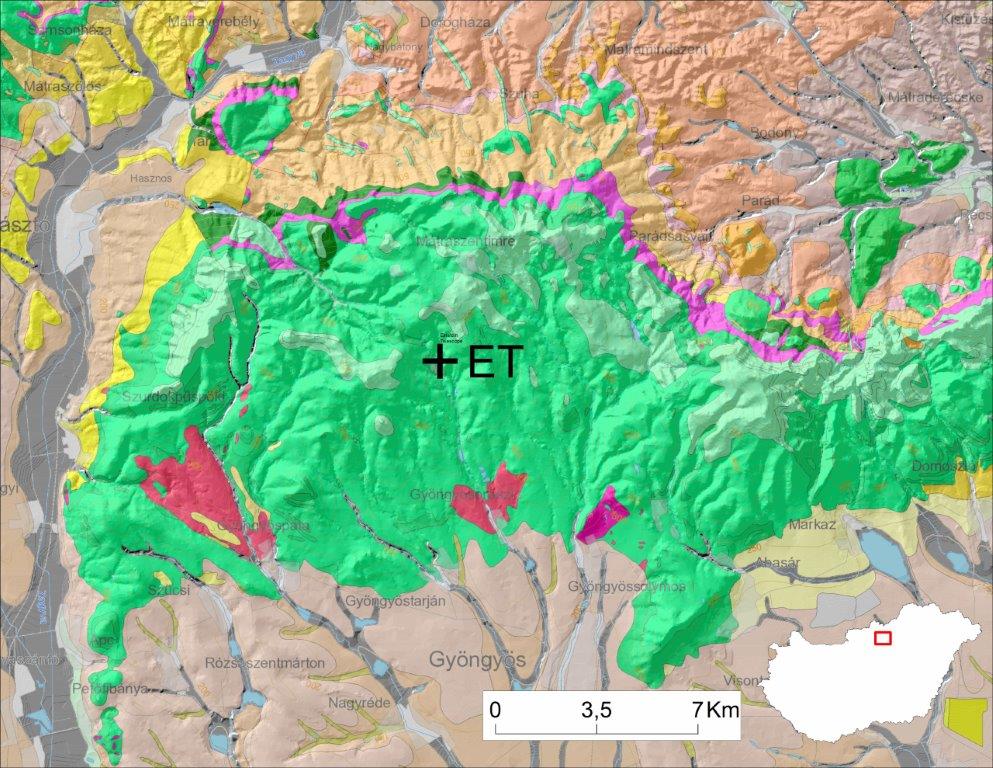
Figure 1. The surface lithology of the Mátra area. The green part denotes various andesitic rocks.

2.1. Seismicity of the Mátra Mountains and the surrounding areas

In general earthquakes are more important for the stability of the underground facility and small ones are not critical regarding the observations.

The seismicity of the Carpathian basin as a whole can be considered moderate. The known earthquakes of the area with magnitude larger than 3.0 are shown in Fig. 3. According to the historical collected data on average one earthquake with magnitude $M\geq 5.0$ can be observed in the Carpatho-Pannonian region annualy. Also the seismic activity from neighbouring open pit mines can be identified by the ET1H seismological station deployed in the MGGL with the help of the stations of the Hungarian National Seismological Network [14].

The level of seismic activity in the Mátra Mountains is quite low. Fig. 2 shows the epicentres of the known $M\geq 3$ earthquakes in the area (19.69-20.18E, 47.8-48.0N) based on the data of the MTA CSFK GGI Earthquake Catalogue [12] and Hungarian National Seismological Bulletins [13]. Only earthquakes with magnitude greater than 3.0 are shown as lower magnitude events can be misclassified quarry explosions. It can be seen that only three small earthquakes ($M\leq 3.5$) were ever observed in the area which occurred in 1879, 1895 and 1980.

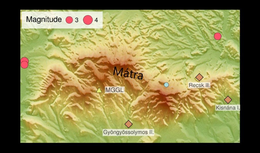
Figure 2. The Mátra area. The triangle shows the location of the MGGL, while the diamonds mark the position and name of the most active quarries. Red circles: known earthquakes in the area.

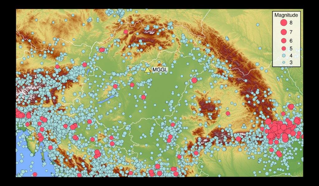
Figure 3. Seismic activity in the Carpatho-Pannonian area. The triangle shows the location of the MGGL. The circles mark the epicentres of the known earthquakes occurred between the years 1800 and 2010. Blue circles: earthquakes with magnitudes 3.0$\leq$M<5.0, red circles: earthquakes with magnitudes M$\geq$5.0.

2.1.1. Ground displacements caused by seismic events

We have selected four events to characterise the ground displacement in the MGGL caused by different seismic events. For the computations of displacements 100 sps streams were used. The data before the instrument correction were detrended and filtered by a second order high pass Butterworth filter with a corner frequency of 1 Hz.

As the seismicity in the Mátra area is mainly determined by the mining activities in the quarries, we computed the ground displacement for characteristic explosions carried out in the three most active mines. Table 1 shows the maximum displacement amplitudes for the three components in the case of the selected events. The magnitude of the displacement is similar for the mines Gyöngyössolymos and Kisnána, while the maximum displacement for the explosion belonging to Kisnána mine is an order of magnitude smaller.

As the recent Tenk earthquake (2013-04-22, M=4.8, epicentral distance=42 km) occurred relatively close to the MGGL it may be of interest. Unfortunately, at the time of the earthquake the ET1H station was not yet installed. However we can use the data of Piszkéstető station, which is located on the surface, 4.88 km from MGGL and was operational. The fourth row of Table 1. shows the displacements observed there. It can be seen that the Tenk earthquake produced around 20-30 times larger displacements than the strongest explosion. It must be noted that in the MGGL - due to the large subsurface depth - this value probably would have been smaller.

Table 1. Observed maximum ground displacement values for frequencies larger then 1 Hz in the case of four characteristic events.

Station	Event	Z [$\mu m$]	N [$\mu m$]	E [$\mu m$]
ET1H	2016-05-10 10:47 (explosion; Gyöngyössolymos; dist= 7.4 km)	0.88	0.66	0.53
ET1H	2017-05-30 10:43 (explosion; Kisnána; dist=21.5 km)	0.10	0.07	0.08
ET1H	2017-06-22 11:21 (explosion; Recsk; dist=16.8 km)	0.34	0.78	0.43
PSZ	2013-04-22 22:28 (earthquake; M= 4.8; Tenk; dist=42.0 km)	20.76	22.57	15.99

2.1.2. Seismic hazard in the Mátra Mountains

The SHARE (Seismic Hazard Harmonization in Europe) was a large-scale collaborative project under the European Community’s Seventh Framework Program [15]. Its main objective was to construct a community-based seismic hazard model for the Euro-Mediterranean region. Its product, the 2013 Euro-Mediterranean Seismic Hazard Model (ESHM13) provides, among others, ground motion hazard maps for the peak ground acceleration (PGA) for different exceedance probabilities. The hazard values are referenced to a rock velocity (vs30) of 800 m/s.

For the Mátra area we obtained the mean PGA values of the SHARE Mean Hazard Model from the online data resource [16] for 73, 102, 475, 975 and 2475 years return periods (Table 2.). These correspond to 50%, 39%, 10%, 5% and 2% exceedance in 50 years, respectively.

Table 2. Average peak ground accelaration values in the Mátra Mountains for different return periods according to the SHARE Mean Hazard Model

Return period [years]	PGA [$m/s^{2}$]
73	0.016
102	0.021
475	0.051
975	0.077
2475	0.123

2.2. Elastic and rheological properties of andesite from Gyöngyösoroszi

In the following we give the static and dynamic elastic moduli of the andesitic rock of the Gyöngyösoroszi mine from time dependent laboratory experiments. We interpret these measurements in a rheological modelling framework and justify the obtained model parameters with elastic propagation speed measurements of the P and S waves. These investigations show that the hard rock of Mátra cannot be considered ideal elastic in a characteristic frequency range. The influence of this property for Newtonian noise should be investigated.

2.2.1. Measured elastic moduli and rheological parameters

As it is well known, the static elastic moduli of rocks measured in laboratory are different from the dynamic ones determined from wave propagation speeds [17, 18, 19, 20, 21, 22]. The difference is usually attributed to various heterogeneities, like microcracks, porosity and grain structure. The Kluitenberg-Verhás body of thermodynamic rheology, which is derived from non-equilibrium thermodynamics with internal variables, provides a simple modelling possibility and explanation [23, 10]. If the material relaxation times of geometric effects are in the order of the operational domain of the low frequency part of ET, then rheological properties can influence the reliable detection of gravitational waves. Therefore we have performed laboratory measurements in order to determine the rheological properties of the gray andesite of Mátra.

The investigated samples were cutted from blocks originated in construction works at the vicinity of MGGL. This is a middle gray, small grained, isotropic piroxen type andesitic rock, which is a differentiated upper miocen (tortona type), about 14.5 million years old and considered typical in this region.

The measurements were performed in the rock mechanics laboratory of Kőmérő Ltd.  with the help of a hydraulic instrument (maximal compression is 150kN), HBM C6A (1MN) load sensor and a HBM Spider 8 & CatmanEasy collected the data. The diameter and the lengh of the cylindrical sample was $37.99$ mm, and $78.33$ mm and its mass was $0.2213$ kg. The uploading speed was $0.7$ kN/s in every cycles. A hysteresis type measurement with increasing stress amplitudes was chosen to determine rheological parameters. In our calculations only the uploading parts of the last two cycles are considered.

The force and the axial deformation are shown on the left side of Fig. 4 as functions of time. The right side of Fig. 4 shows the axial stress as function of axial and lateral deformations at the positive and negative horizontal axes, respectively. The rheological hysteresis and also the apparent permanent deformation is visible at the end of creep periods. Therefore andesitic rocks from Mátra show clear deviation from ideal elasticity with properly designed laboratory experiments.

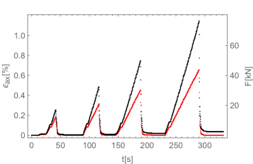
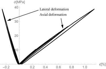
Figure 4. Left panel: Axial deformation (black) and loading force (red) with constant uploading speed as function of time. Right panel: Axial stress as function of the axial and lateral deformations (positive and negative horizontal axes, respectively) with hysteresis curves of rheological origin.

2.2.2. Kluitenberg-Verhás body and static-dynamic elasticity

The isotropic Kluitenberg-Verhás body is given by the following relations between the stress $\sigma$ and strain $\epsilon$:

$$\tau_{d}\dot{\sigma}_{d}+\sigma_{d} = E_{2d}\ddot{\epsilon}_{d}+E_{1d}\dot{\epsilon}_{d}+E_{0d}\epsilon_{d},$$ (1)

$$\tau_{s}\dot{\sigma}_{s}+\sigma_{s} = E_{2s}\ddot{\epsilon}_{s}+E_{1s}\dot{\epsilon}_{s}+E_{0s}\epsilon_{s}.$$ (2)

Here the dot denotes time differentiation, the subscripts $d$ and $s$ refer to the deviatoric and spherical stresses and deformations as well as to the related material parameters, like the $\tau_{d}$ and $\tau_{s}$ deviatoric and spherical relaxation times. In our case a cylindrical laboratory sample was prepared according to ISRM (International Society of Rock Mechanics) standards, therefore the uniaxial stress, $\sigma$, and the axial and lateral deformations $\epsilon_{a}$ and $\epsilon_{l}$ determine the spherical and deviatoric stresses and strains as $\sigma_{d}=2\sigma/3$, $\sigma_{s}=\sigma/3$, $\epsilon_{d}=2(\epsilon_{a}-\epsilon_{l})/3$ and $\epsilon_{s}=(\epsilon_{a}+2\epsilon_{l})/3$.

The elastic moduli $E_{0d}=2G$ and $E_{0s}=3K$ are the well known static Lamé coefficients and $E_{1d}$ and $E_{1s}$ are the deviatoric and spherical viscoelastic material coefficients. If the $E_{2d}$ and $E_{2s}$ dynamic parameters are neglectable, then the Kluitenberg-Verhás body simplifies to the Poynting-Thomson-Zener body [23], which is the standard model of creep and relaxation phenomena in rock mechanics (also with the names generalized Kelvin-Voigt and Hill-Maxwell body [24]). Then it is convenient to transform equations (1) and (2) into a hierarchical form:

$$\tau_{d}\dot{\sigma}_{d}+\sigma_{d}-E_{1d}\dot{\epsilon}_{d}-E_{0d}\epsilon_{d} = \tau_{d}\frac{\rm d}{{\rm d}t}\left(\sigma_{d}-b_{d}E_{0d}\epsilon_{d}\right)+\sigma_{d}-E_{0d}\epsilon_{d},$$ (3)

$$\tau_{s}\dot{\sigma}_{s}+\sigma_{s}-E_{1s}\dot{\epsilon}_{s}-E_{0s}\epsilon_{s} = \tau_{s}\frac{\rm d}{{\rm d}t}\left(\sigma_{s}-b_{s}E_{0s}\epsilon_{s}\right)+\sigma_{s}-E_{0s}\epsilon_{s}.$$ (4)

Here the parameters $b_{d}=E_{1d}/(\tau_{d}E_{0d})$ and $b_{s}=E_{1s}/(\tau_{s}E_{0s})$ measure the deviation from the ideal elastic Hook body. If $b_{d}=b_{s}=1$, then the material is apparently completely elastic. The propagation speed of longitudinal and transversal waves determine the material parameters, $E_{d,dyn}=b_{d}E_{0d}$ and $E_{s,dyn}=b_{s}E_{0s}$, respectively. These are called dynamic Lamé coefficients. Both for the static and dynamic cases the Young modulus and the Poisson coefficient are calculated from the Lamé coefficients as $Y=3E_{s}E_{d}/(2E_{s}+E_{d})$ and $\nu=(E_{s}-E_{d})/(2E_{s}+E_{d})$.

2.2.3. Material parameters

One can determine the static and dynamic elastic moduli both from the cyclic loading of the sample given above and the dynamic ones can be determined from direct laboratory measurements of the sound speeds. This direct laboratory measurement of the propagation speed of longitudinal and transversal waves gives the dynamic Young modulus $(38.6\pm 1.1)$ GPa, and the dynamic Poisson coefficient $0.18\pm 0.01$.

Furthermore, the time dependent data of the chosen rock sample was analysed using the differential equations of the rheological models. In particular we have assumed, that the measured deformation values are given and we have determined the best parameters from the differential equations (1) and (2) of the Kluitenberg-Verhás body to obtain the stress, both for the deviatoric and spherical components. According to these calculations the coefficents of the second derivatives of the deformation, the $E_{2d}$ and $E_{2s}$ coefficients, can be neglected and the Poynting-Thomson-Zener model, (3) and (4), was applied. The obtained best fit parameters are shown in Table 3.

Cycle 3 up	$E_{d}=2G$ [GPa]	$E_{s}=3K$ [GPa]	$E_{Young}$ [GPa]	$\nu$
static	$23\pm 2$	$33.9\pm 0.5$	$25\pm 2$	$0.13\pm 0.03$
dynamic	$32\pm 4$	$73\pm 1$	$39\pm 4$	$0.23\pm 0.03$
Cycle 4 up
static	$17\pm 5$	$50.1\pm 0.3$	$22\pm 5$	$0.28\pm 0.05$
dynamic	$27\pm 5$	$58\pm 3$	$33\pm 5$	$0.22\pm 0.05$

Table 3. The static and dynamic elastic coefficients according to rheological data evaluation of the uploading parts of the 3^th and 4^th cycles of the laboratory experiment. The dynamic Young modulus and dynamic Poisson ratio $\nu$ are consistent with the values obtained from propagation speeds of the P and S waves.

	$b_{d}$	$b_{s}$
Cycle 3	$1.4\pm 0.2$	$2.15\pm 0.05$
Cycle 4	$1.6\pm 0.6$	$1.16\pm 0.06$

Table 4. The rheological parameter, $b=\frac{E_{1}}{E_{0}\tau}$, characterising the deviation from the ideal elastic regime both in the deviatoric and spherical cases.

Fig. 5 shows the measured stress values and also the stress determined from the rheological model with the parameters above for the uploading part of the third and fourth cycles in the deviatoric case. The deviation of the two curves from the data is below 0.05 MPa in the whole domain.

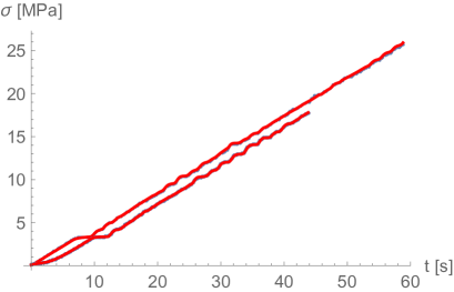
Figure 5. The deviatoric stress as the function of time in the uploading part of the third and fourth loading cycles. The the blue data points are under the solid red fitted model solution curve.

According to our measurements the typical gray andesite of Mátra is not ideally elastic and the deviation from elasticity is of rheological origin. The experimental parameters can be obtained both from the wave propagation speed measurements and from the cyclic loading experiments. These coefficients are consistent as it is shown by our preliminary calculations. The obtained transition regime, which is proportional to the inverse relaxation times, is 0.02-0.1Hz, which is below the low frequency sensitivity of ET. However, our experimental methodology prevents the detection of faster relaxation modes, therefore further investigations are necessary.

3. Seismological measurements I.

The ET site selection preparation measurements [9, 25, 26] selected three best candidate sites for the Einstein Telescope in Europe. The selection is based on the low seismic noise level in the critical low frequency range 1-10Hz. The survey investigated several underground locations, each of them about for a week. In order to have a better estimate of the average seismic noise it is reasonable to collect at least two years of data and analyse the annual and seasonal changes in noise level originating from natural sources and human activity. The above mentioned survey was the main motivation in the establishment of MGGL. Due to the ongoing reclamation activity in the Gyöngyösoroszi mine the vicinity of the laboratory was also subject of maintenance works. Therefore in our case both internal and external human activities were contributed to the noise level.

Seismological data collection was performed by two Guralp CMG 3T low noise, broadband seismometers [10], and also by the custom made seismic sensor developed in the Warsaw University. The Guralp instruments are sensitive to ground vibrations with flat velocity response in the frequency range 0.008-50 Hz. The Guralp seismometers were calibrated and cross calibrated, operated according to protocol of the seismometers in the Hungarian National Seismological Network. The self noise of the seismometers was below the low noise model from 0.02 Hz to 10 Hz [27].

The custom made Warsaw seismometer uses one vertical and two horizontal geophone sensors mounted firmly in a single aluminium block placed inside a metal housing along with a data acquisition system. The geophones (LGT-2.5 and LGT-2.5H) used as the sensors have the lower corner frequency of 2.5 Hz. The data acquisition system sampled the analog signal with the frequency of 125 Hz and the 32-bit resolution. The Warsaw seismometer was calibrated by comparing the data with a Trillium seismometer, and also with a Guralp CMG 3T during a data calibration session at the MTA Wigner Research Centre for Physics in January 2015.

One of the Guralp instruments (ET1H) and the Warsaw seismometer (WARS) were permanently installed in the MGGL. The seismometers were deployed on separated concrete piers which were connected to the bedrock. Between the piers and the seismometers a granite plate has been placed. The other Guralp instrument (hereafter GU02) was used in a measurement campaign in the first two weeks of June 2017 in a measurement cabin, constructed next to the main tunnel and prepared for seismometer installation. The mutual performance of the ET1H and WARS seismometers are demonstrated on Fig. 6, where the averages of the day 2017-07-01 and 2017-07-02 are calculated for each instruments and also the ratio of the averages at given frequency range. The agreement is similar to other customary chosen days during the measurement campaign. Therefore the cross-calibration of the instruments is satisfactory.

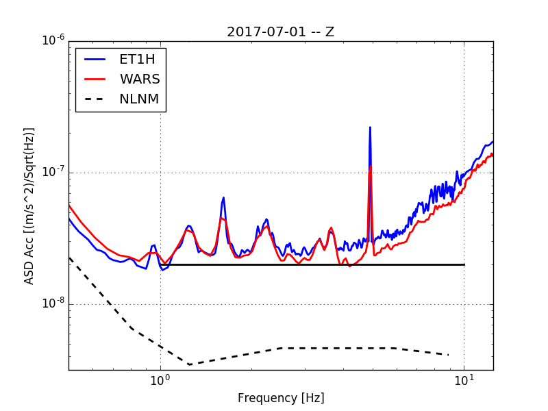
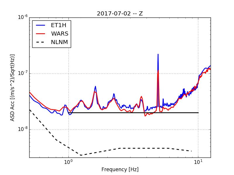
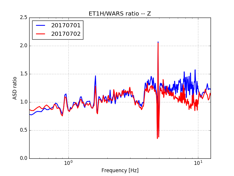
Figure 6. The daily average ASDs of 2017-07-01 and 2017-07-02 from the data of ET1H and the Warsaw seismometer, Z direction. The last figure shows the ratio of ASDs for the two studied days.

The data acquisition period of the two instruments slightly differs due to operational problems, however the amount of the collected data is similar. In the following first we analyse the ET1H data, then the WARS data. The methods and the elaboration are different, in order to show more aspects of the noise measurements.

3.1. Run-1 data analysis of the ET1H seismometer

The data collection period for ET1H was started on 2016-03-01 and in this paper we elaborate the data until 2018-06-28. From the point of view of ET related data the instrument was out of order in the periods 2016-09-09 — 2016-09-18, 2016-10-13 — 2016-10-16, 2016-10-19 — 2016-11-16, 2017-12-16 — 2018-01-31, 2018-03-14 — 2018-04-04 and 2018-04-13 for ET1H. The Z direction data was compromised between 2016-09-22 —2016-10-16, for 25 days. Therefore 741days of data was collected for the horizontal directions and 716 days in the vertical direction. In our analysis we followed the data processing method of Ref. [26]. The particular problems observed in long term data analysis suggested some methodological improvements, and additional characteristics. These were reported in Ref. [28] where the precise definitions and the justification of the methodology of data processing can be found. In this section some basic definitions are recalled for clarification.

The velocity Power Spectral Density (PSD) is defined as [26, 28]

$$P^{(v)}=\frac{2}{f_{s}\cdot N\cdot W}\left|V_{k}\right|^{2},$$ (5)

where $f_{s}$ is the sampling rate — in our case it is $100$ Hz —, $N$ is the length of the analysed data sample — $N\,=\,5000$ —, and $W=\frac{1}{N}\sum_{n=1}^{N}w[n]^{2}$ with the Nuttall window function $w[n]$. We did not use the advantage of fast Fourier algorithm on the expense of increasing the lowest frequency value. The coefficients $V_{k}=F(w[n]\cdot(v[n]-\langle v\rangle)$, represent the Fourier transform of the deviation of raw velocity data $v[n]$ from its average value $\langle v\rangle$. In our analysis PSD-s were calculated with 50 s data samples with $f_{s}=100$ Hz sampling rate. Before further processing, raw data were highpass-filtered with $f_{HP}=0.02$ Hz and the overlap is 3/4 due to the window function. To characterize spectral properties the acceleration Amplitude Spectral Density (ASD),

$$A^{(a)}=A=\sqrt{P^{(v)}\cdot\omega^{2}}$$ (6)

will be used and displacement $rms$ will be applied as cumulative property. This is the square root of the integral of displacement PSD between two frequency values

$$rms=\sqrt{\frac{1}{T}\sum_{k=l}^{K}P_{k}^{(v)}/\omega^{2}},$$ (7)

where $l$ is the low cut-off index — in Beker’s paper this is chosen to be $2$ Hz —, the $K$ is the high cut-off index — usually the Nyquist frequency — and $T=\frac{N}{f_{s}}$. In our case $l$ is chosen to be $1$ Hz or $2$ Hz and $K$ is either the Nyquist-frequency or $10$ Hz, because we use $rms_{2Hz}$ of Beker and also calculate the $rms_{2-10Hz}$ and $rms_{1-10Hz}$ values. With these new measures we can drop the irrelevant frequency interval above $10$ Hz and consider the technologically already available $1-2$ Hz region [28]. The commonly used comparative measure for the spectral properties of the sites is a particular value of the amplitude spectral density, the so called Black Forest line:

$$A_{BF}=2\cdot 10^{-8}{\rm\frac{m/s^{2}}{Hz}}.$$ (8)

It is worth to give the various rms values corresponding to the the reference spectral density represented by the Black Forest line: $rms_{2Hz}^{BF}\approx 0.1\,nm$ $rms_{2-10Hz}^{BF}=0.1\,nm$ and $rms_{1-10Hz}^{BF}=0.29$ nm.

An other important aspects of the long term data evaluation are the use of percentiles and the choice of intermediate averaging periods. Previous studies applied the mode of the data for the representation of a characteristic mean value. However, the median, and also the other percentiles, are less sensitive for discretisation and the inevitable averaging. Moreover, naturally select the representative data without a necessity of filtering short large noise bursts. Therefore in the following the analysis of site properties is mostly based on the median of the data. However, we will demonstrate the most important differences in the spectral representation and also calculate the mode related $rms_{2Hz}$ of Beker for a clear comparison with the previous studies.

It is also worth to mention, that the basic Fourier length used at the Fourier transformation was 50 s for Guralp instruments and 128s for WARS. For the ET1H and GUO2 Guralp instruments we have introduced a short time averaging (STA) period of $300\,s$ and for the two-year data the use of daily averages was convenient. The daily periods were called intrinsic averaging (INA), because it considers the natural periodicity of the data. In other words in order to obtain the long term $10\textsuperscript{th},50\textsuperscript{th}$ and $90\textsuperscript{th}$ percentiles first the short therm averages (STA) were calculated and then particular chosen periods in each day (INA) enable the comparison of working hours, night time or whole day data. See [28] for more details about the chosen methodology.

3.2. Long term seismic results

A particular factor in our noise analysis is the ongoing mine reclamation activity in the Gyöngyösoroszi mine. As a result, the investigation and identification of various noise sources originating from external and internal human activity, machine noise, construction works, train noise, etc. proved to be difficult. In November 2016 a three-shift operation period has been started with increased industrial noise, present also during the nights. In order to compare the noise types of these kind of activities in our analysis we have defined three periods for each day for our study: (a) the whole day, (b) night period (20:00 - 2:00 UTC) and (c) working period (9:00 - 15:00 UTC). In the following we present a comparative analysis of long term data considering seasonal changes, external and internal human noise and also depth dependence for a shorter two weeks long measurement campaign performed by our second Guralp instrument, GUO2, at -404 m depth.

3.2.1. Complete Run-1 results

The acceleration ASD-s for the two-year observation period are shown in Fig. 7. The borderlines of the blue colored area are the 10^th and 90^th percentiles of daily $300$ s data. The dotted black lines are the modes of the $1800$ s averages, according to the methodology in Ref. [25]. The medians and modes are closer to the Black Forest level in horizontal directions. It is also remarkable that the mode underestimates the median, that is most of the days are noisier than the mode. at a given frequency. This is well represented in the corresponding $rms$ values given in Tab. 5, too. Here the first line $rms_{2Hz}$, calculated from the mode of the data. It is worth to recall that it was $0.12$ nm in the previous short term measurements of Beker in the same place. As it can be seen, the $rms$ calculated from the median is much larger, about $20\%$ more. It is also worth to mention that the Black forest line reference value of $rms_{1-10Hz}$ is $0.29$ nm, and the $rms_{1-10Hz}$ normalized to this value is less than the $rms_{2-10Hz}$, therefore the site is less noisy at the lower frequencies, as it can be seen in Figs. 7, as well.

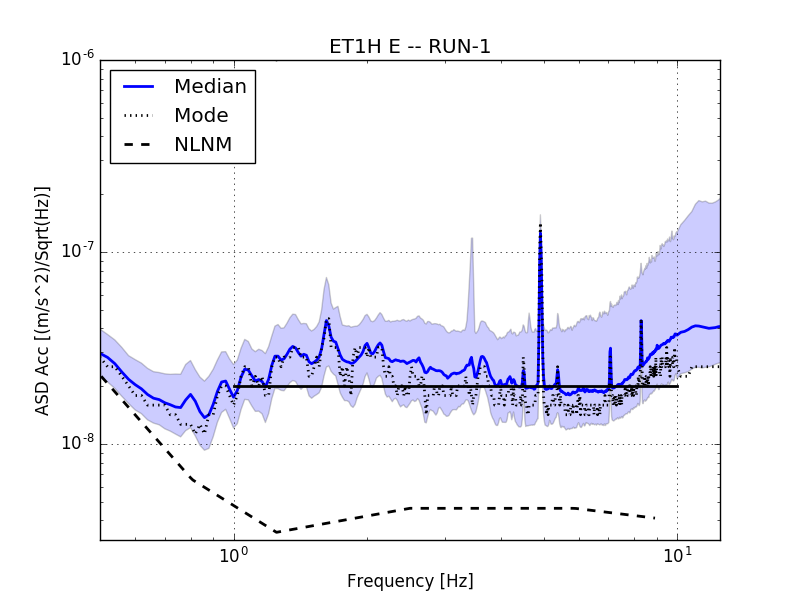
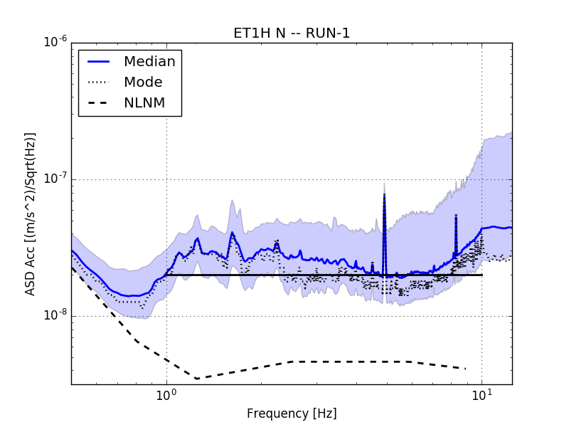
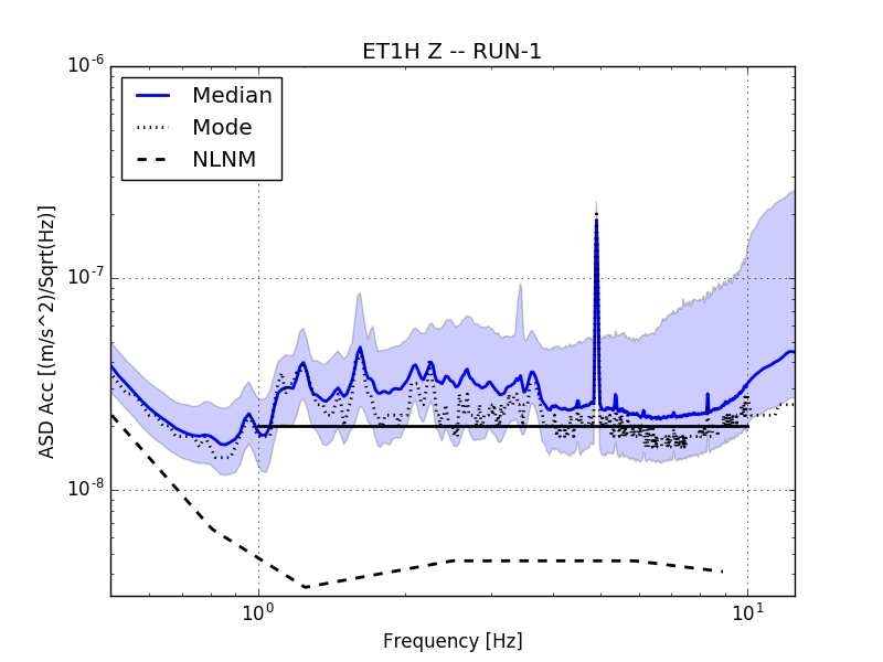
Figure 7. The acceleration ASD spectra of the East-West (ET1H E), North-Sud (ET1H N) and in the vertical directions (ET1H Z). The solid blue and the dotted black lines indicate the median and the mode of the the data, repectively. The borderlines of the blue colored area are the 10^th and 90^th percentiles. The Black Forest line is solid black and the dashed black lines show the New Low Noise Model of Peterson (NLNM) [29].

Whole day	East	North	vertical
Mode $rms_{2Hz}$	0.123	0.121	0.140
Median $rms_{2-10Hz}$	0.144	0.147	0.176
Median $rms_{1-10Hz}$	0.387	0.417	0.436

Table 5. The various $rms$ values in nm of Figs. 7 are shown. The reference value for the Black Forest line is $0.29$ nm for $rms_{1-10Hz}$.

The role of the human and industrial noises is shown in Fig. 8, where the spectral densities for the working and night periods is plotted in the North-South and the vertical directions. It is remarkable, that half of the frequency range is below the median of the data (blue line), the asymmetric relative position of the blue area at working period indicates the presence of short noisy periods between 9:00 - 15:00 UTC. We have to mention that from the end of 2016 the reclamation works were performed close to the MGGL in a three-shift schedule.

In order to illustrate the cultural and industrial noises the frequency dependence of the ratio of the working and night periods are plotted in Fig. 8. The cultural noises start at about $0.7$ Hz and reach their maxima between $2-3$ Hz and $10-20$ Hz. We may suppose that the night shifts cause less noises, the main works are done during the daytime. Then the observed noise level at the night periods can be considered as an upper limit for an operating underground GW detector facility, where the equipments are optimized for a low noise operation.

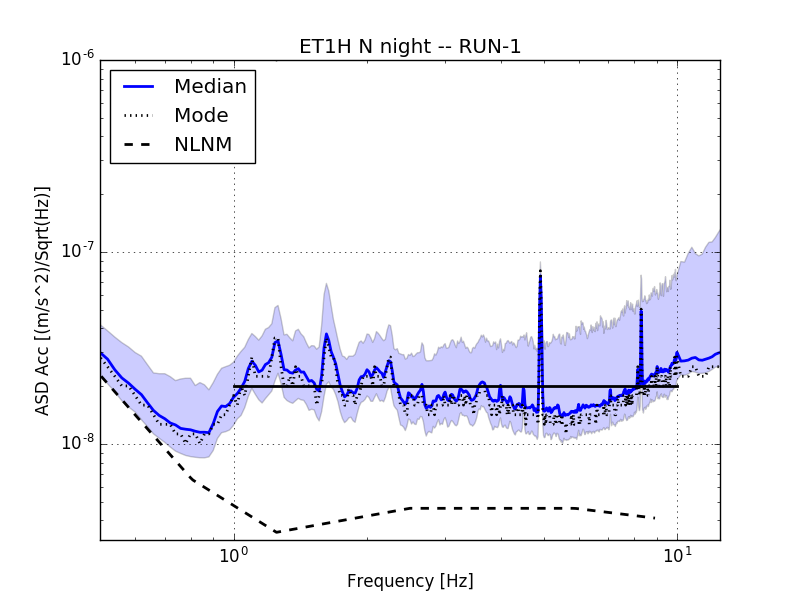
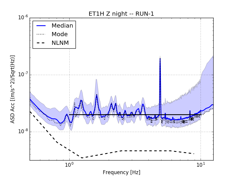
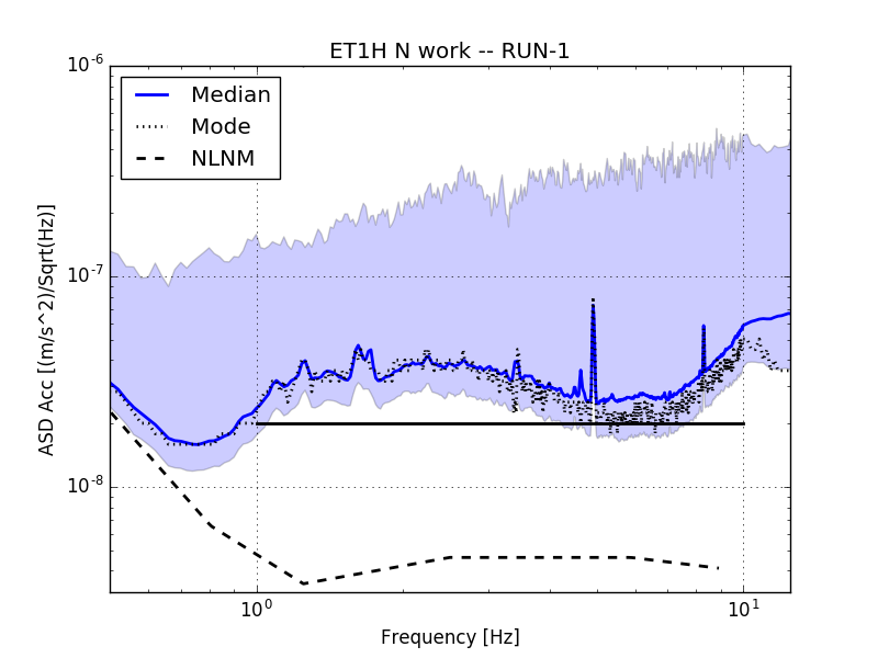
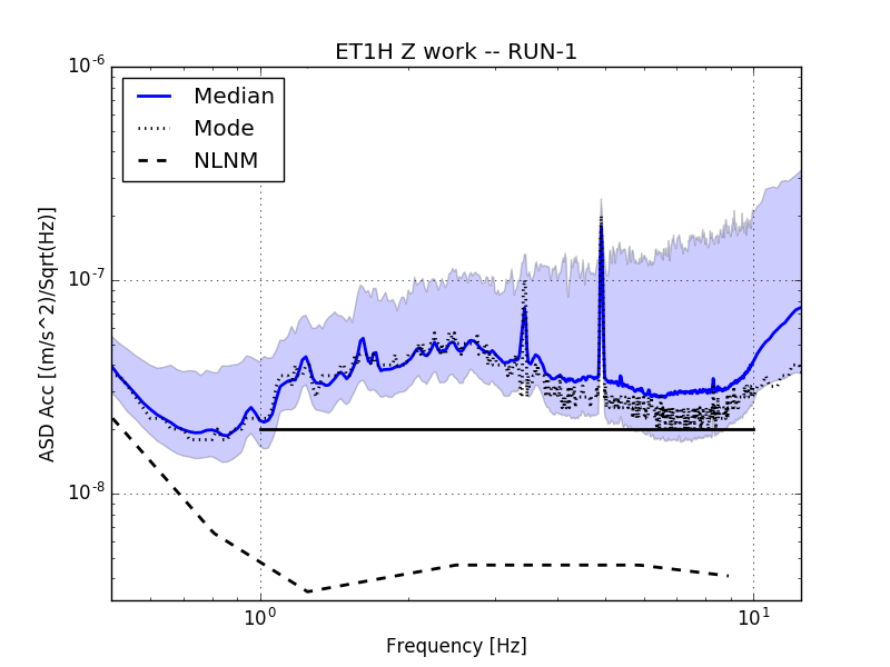
Figure 8. The acceleration ASD-s of the working and night periods of 741 days data for a horizontal and the vertical directions. The solid blue and the dotted black lines indicate the median and the mode of the the data, repectively. The borderlines of the blue colored area are the 10^th and 90^th percentiles. The Black Forest line is solid black and the dashed black lines are NLNM curves.

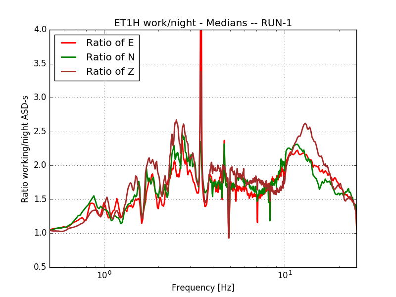
Figure 9. The frequency dependence of the ratios of the night and work period medians in the three directions.

The corresponding $rms$ values are for the night and working periods are given in Table (6. We can see, that the $rms$ of the noisier working periods can be two times higher than in the calm night ones.

Night period	East	North	Z
Mode $rms_{2Hz}$	0.101	0.102	0.123
Median $rms_{2-10Hz}$	0.114	0.115	0.128
Median $rms_{1-10Hz}$	0.324	0.354	0.353

Working period	East	North	Z
Mode $rms_{2Hz}$	0.196	0.189	0.240
Median $rms_{2-10Hz}$	0.193	0.147	0.241
Median $rms_{1-10Hz}$	0.456	0.490	0.527

Table 6. The $rms$ values in nm for the night and working periods in Run-1, according to the panels of Fig. 8.

The differences at longer periods in Run-1 were analysed by three different methods. First, the acceleration ASD-s of the night periods were plotted for each year in Fig. 10. The $90\textsuperscript{th}$ percentiles at higher frequencies show the increasing industrial noise at night due to the three-shift schedule of the mine works. Interestingly this is not apparent in the mode and in the median of the data, because the particular activity seemingly put up only short noisy periods. In Table 7 the $rms_{2-10Hz}$ values of the night periods of each year are shown, corresponding to the middle panels of Fig. 10. There is no significant annual variation during Run-1 of MGGL.

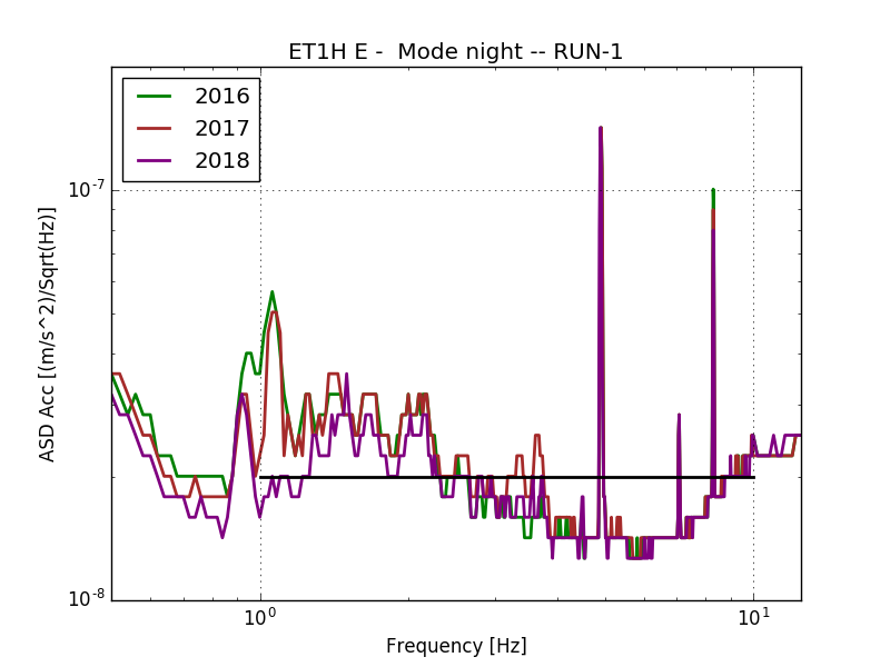
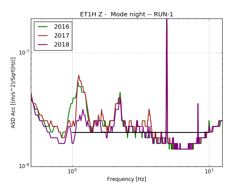
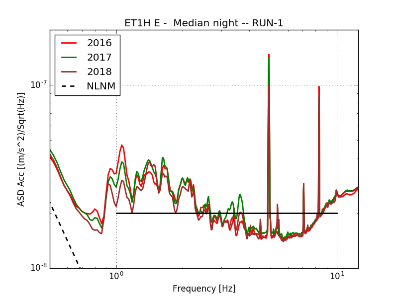
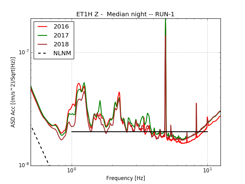
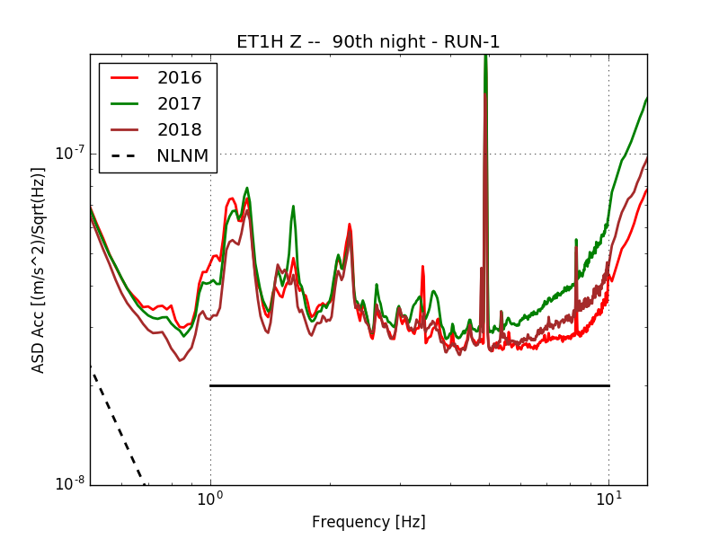
Figure 10. The acceleration ASD-s for the years 2016, 2017 and 2018. The upper panels show the modes, the two figures in the middle row is for medians and the bottom graphs are the $90\textsuperscript{th}$ percentiles for each year. The Black Forest line is solid black and the dashed black lines are NLNM curves.

Night	2016	2017	2018
E	0.124	0.127	0.123
N	0.122	0.123	0.128
Z	0.149	0.151	0.137

Table 7. The median $rms_{2-10Hz}$ values in nm of the night periods in the years of Run-1.

The seasonal averages are plotted in Fig. 11 including the $rms$ values in Table 8, which presents that the calmest seasons are the spring and the summer.

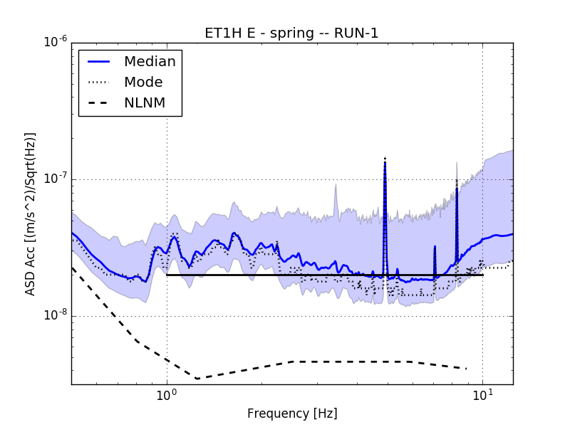
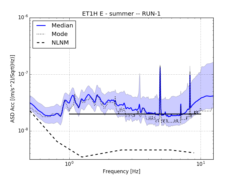
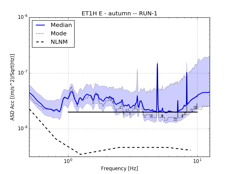
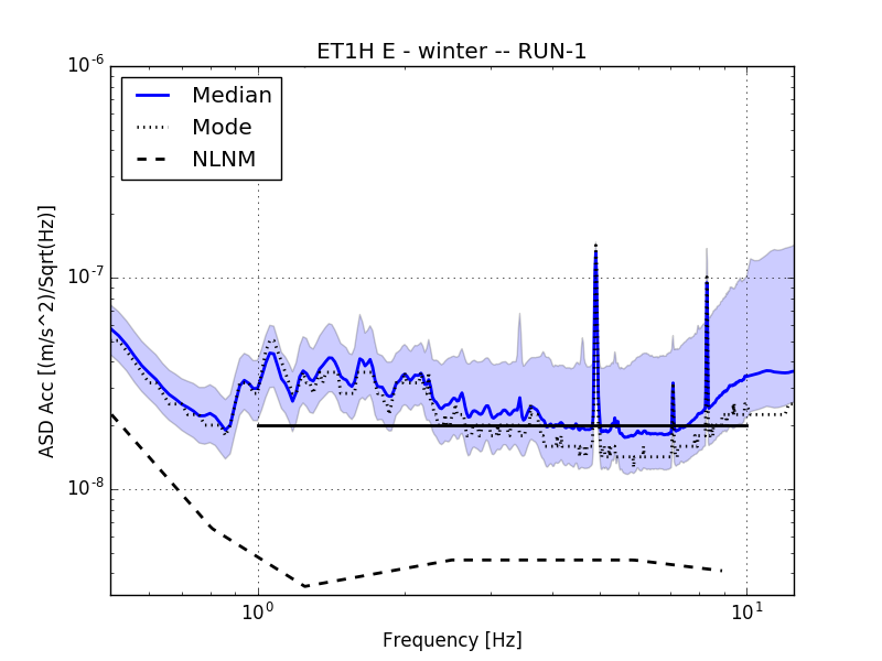
Figure 11. The acceleration ASD of the different seasons for a horizontal component calculated is shown here from whole-day periods. The solid blue and the dotted black lines indicate the median and the mode of the data, respectively. The borderlines of the blue colored area are the 10^th and 90^th percentiles. The Black Forest line is solid black and the dashed black lines are NLNM curves.

$rms_{2Hz}[nm]$	spring	summer	autumn	winter
E	0.125	0.134	0.139	0.132
N	0.122	0.130	0.131	0.130
Z	0.148	0.164	0.169	0.160
$rms_{1-10Hz}[nm]$	spring	summer	autumn	winter
E	0.461	0.522	0.546	0.514
N	0.487	0.557	0.581	0.554
Z	0.505	0.592	0.625	0.599

Table 8. Seasonal variation of the $rms$ values of the seasons according to the data shown in Fig. 11. The first part is the $rms_{2Hz}$ of the mode and the second one is the $rms_{1-10Hz}$ of the median.

Finally, the seasonal changes are represented with a timeline plot of the the daily $rms$ values in Fig. 12. As we can see, there is an annual trend in the curves, the late spring and the early summer are the most silent periods in the $1-10$ Hz frequency range. Note, this seasonal difference is not apparent in the $rms_{2Hz}$ timeline, which is at the bottom panel of Fig. 12. This seasonal variation of the lowest frequency noise is in agreement with the observable also in Fig. 11.

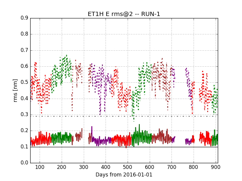
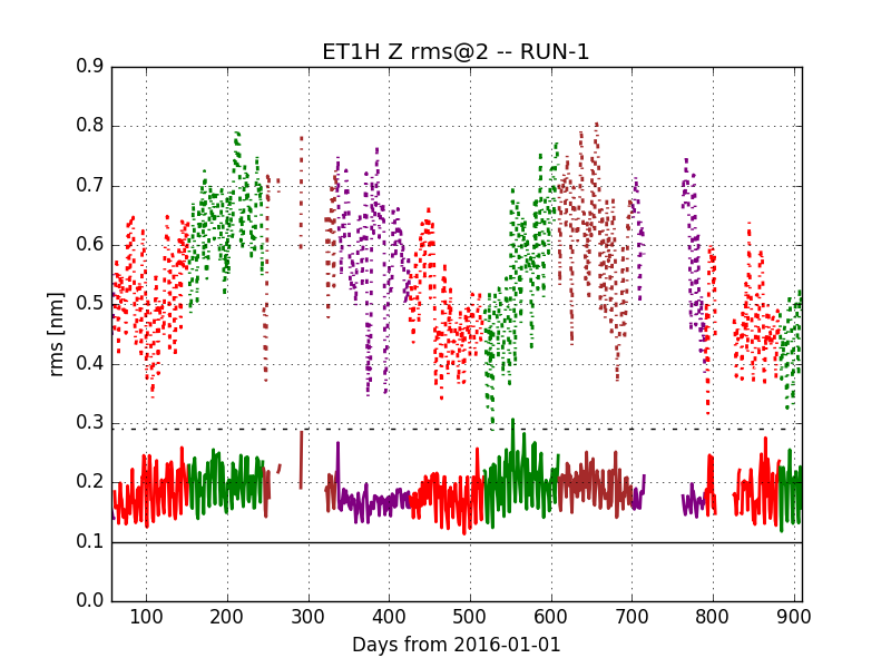
Figure 12. The timeline of the daily $rms$ values for the whole Run-1 in a horizontal and in the vertical direction. In the figures the mode related $rms_{2Hz}$ is the solid line and the $rms_{1-10Hz}$ from median is the dashed one. The colours red, green, brown and purple are for the spring, summer, autumn and winter periods, respectively. The solid and dashed black lines are the referential Black Forest values, $rms_{2Hz}=0.1nm$ and $rms_{1-10Hz}=0.29nm$.

3.2.2. Comparing the deep and shallow

In this section the GU02 (-404 m) results from a two-week observation run (1-15 June 2017) are compared to the parallel close to surface MGGL measurements of ET1H (-88 m). Because of the shorter time interval, the percentiles were computed directly from the $300$ s averages without INA. The modes were calculated from $1800$ s averages as in the previous section. In Fig. 13 the comparison of the two-week and the total Run-1 ET1H data are plotted. One can see, this two-week period is representative, there is no significant differences of the plots, in spite of the INA in case of Run-1.

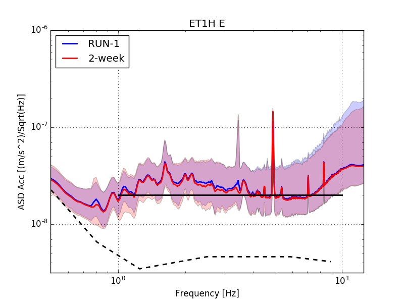
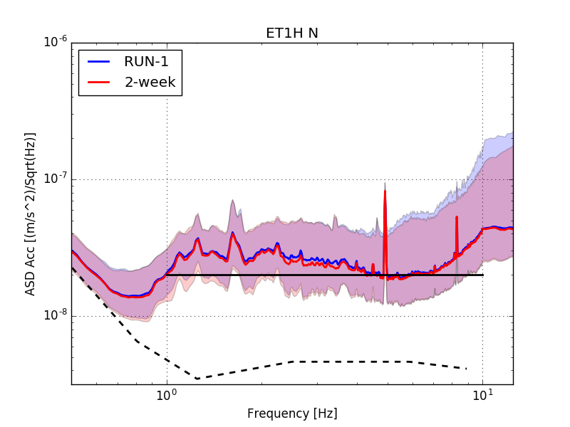
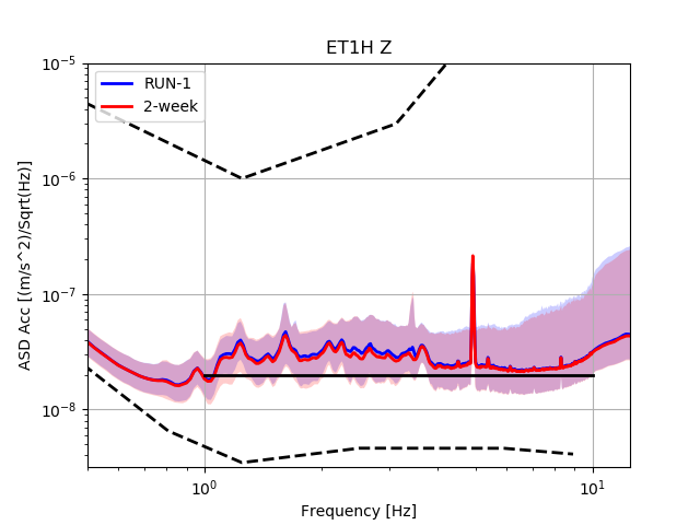
Figure 13. The acceleration ASD of the Run-1 (blue) and the particular two-week periods (red) of the ET1H station in each directions. The borderlines of the coloured areas are the 10^th and 90^th percentiles. The Black Forest line is solid black and the dashed black lines are NLNM curves.

ET1H	$rms_{2Hz}$	$rms_{2-10Hz}$	$rms_{1-10Hz}$
E	0.126	0.140	0.385
N	0.122	0.143	0.417
Z	0.143	0.169	0.427

GU02	$rms_{2Hz}$	$rms_{2-10Hz}$	$rms_{1-10Hz}$
E	0.0829	0.0961	0.259
N	0.0690	0.0951	0.259
Z	0.0690	0.0830	0.363

Table 9. The $rms$ values in $nm$ for the spectral densities in Fig. 14. The $rms_{2Hz}$ is calculated from the mode, the other from the median.

We have plotted together the ET1H and GU02 data in Fig. 14. There it is apparent that the main attenuation is in the intervall of 1-4 Hz for the horizontal and 1-7 Hz for the vertical direction. This interval is crucial for the low frequency noise budget of the proposed ET, furthermore, this frequency range dominate all the $rms$ values. The corresponding $rms$ values for GU02 are in Tab. 9.

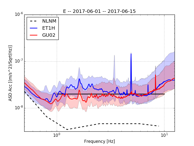
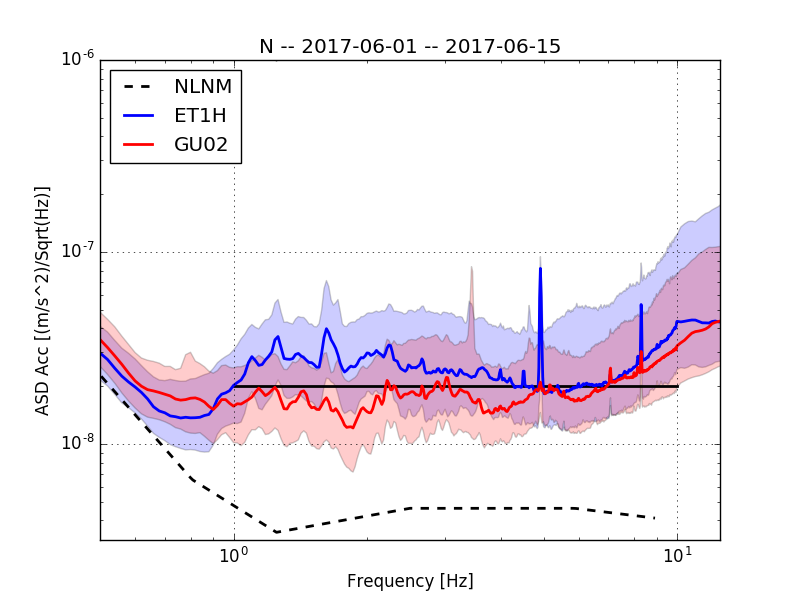
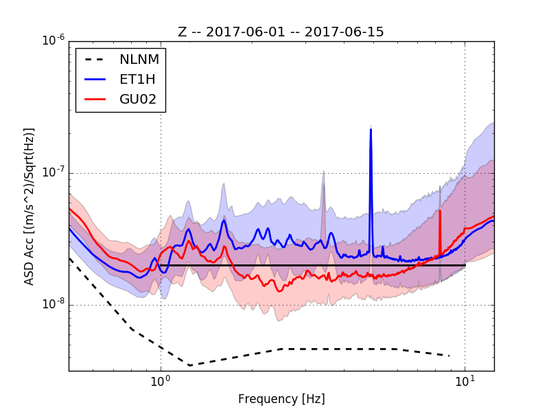
Figure 14. The percentiles of the ET1H $-88$ m and (red) the GU02, $-404$ m (blue) stations are shown together in the three directions. The Black Forest line is solid black and the dashed black lines are NLNM curves.

In Fig. 15 the night and working periods are shown for the GU02 station with the corresponding $rms$ values in Tab. 10. The ratios of night and working periods are also shown in Fig. 16.

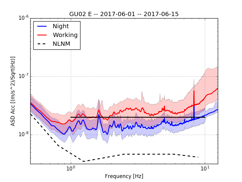
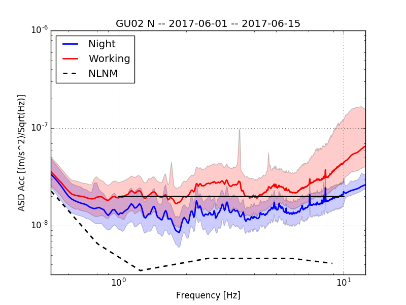
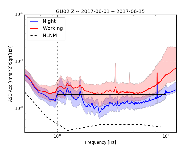
Figure 15. Comparison of the ASD of the night and work periods of the GU02 station. The Black Forest line is solid black and the dashed black lines are NLNM curves.

Night period	$rms_{2Hz}$	$rms_{2-10Hz}$	$rms_{1-10Hz}$
E	0.0748	0.0752	0.217
N	0.0746	0.0732	0.213
Z	0.0625	0.0619	0.304

Working period	$rms_{2Hz}$	$rms_{2-10Hz}$	$rms_{1-10Hz}$
E	0.143	0.135	0.318
N	0.150	0.135	0.326
Z	0.135	0.121	0.431

Table 10. The calculated $rms$ values in $nm$ for the night and working periods of the GU02 station, according to Fig. 16.

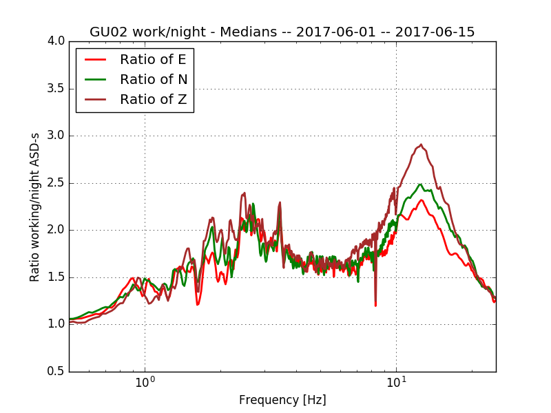
Figure 16. The ratio the noise median in the night and in the working periods for the GU02 station.

3.3. Summary

We analysed the long term Run-1 data of the ET1H station and compared the data from a representative two-week period of the $-88$ m deep ET1H station with the $-404$ m deep GU02 station. For higher than $2$ Hz frequencies, there are no significant annual changes, but for $1-2$ Hz the spring-summer time shows annual minimum. Comparing the deeper and shallower noise data we have observed that the decrease of seismic noise spectral amplitudes in the 1-8 Hz frequency range is approximately $60\%$. This range is crucial for the low frequency performance of Einstein Telescope.

We emphasize, that almost in $90\%$ of the observation period detected the noise level below the Black Forest line at night (see Fig. 15). The related average horizontal $rms_{2-10Hz}=0.0742$ nm and the $rms_{1-10Hz}=0.213$ nm. The first value is equal to the mode related $rms_{2Hz}$ value, which is $0.0745$ nm.

4. Study of seismic noise with the Warsaw seismometer

As it was described in Section 3, the custom made seismometer of the Warsaw University (WARS) is located near to the ET1H seismometer, therefore they should measure the same noise, although at low frequencies there can be differences due to scattering of seismic waves in the mine. The y-axis of the sensor is pointing at the direction of 25 degrees NW.

4.1. The collected and analysed data:

The Run-1 data of the WARS seismometer statts from $24$ May 2016 till $2$ July 2018. In this period 654 days were used for analysis with the rest of the days being unavailable. Days not included in the study will be referred to as “missing-days” henceforth. The data for the study were recorded in each hour. Out of these 654 days, 30 days do not have complete 24 hours and will be referred to as “gap-days” henceforth. After eliminating the missing durationsfrom the gap-days, total of 15 290 hours of complete data were available for analysis.

4.2. Analysis of the WARS data:

The acceleration power spectral density (PSD) [30] was calculated by Welch’s method [31]. The data for each hour were divided into 2048 length segments with each segment windowed by Hann window function [30, 32, 33] using half the length segment as overlap[30]. No zero padding was used. The acceleration amplitude spectral density (ASD) for each hour was calculated by taking square root of the acceleration PSD. The data for each hour were available for each of the three axis for all the 15290 hours so a total of 3$\times$15290 ASDs were generated.

4.3. Monthly analysis of the WARS data:

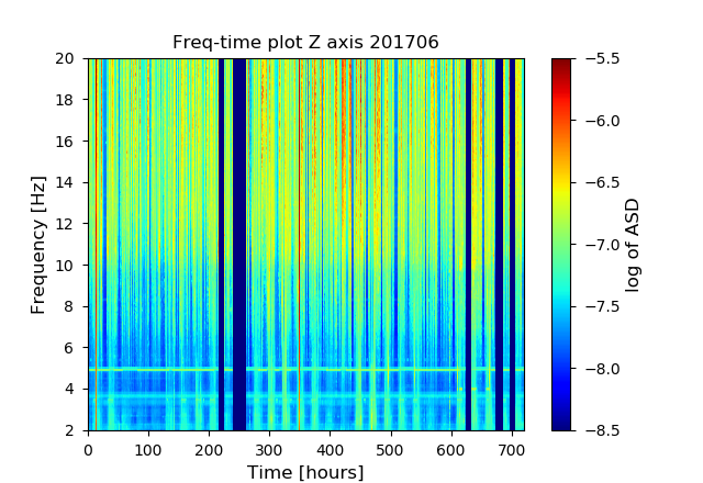
Figure 17. The time frequency plot of the vertical spectrum for June 2017. The daily variation of the noise is clearly seen. The data gaps are in dark blue. Additionally weekends are clearly less noisy - which is seen in the low frequency band. The histogram unit is m$s^{-2}$$Hz^{-1/2}$.

The ASD generated for each hour were used to study the variation of ASDs with time over the period of each month i.e spectrograms were generated for every month for the period of the study. This was done for all three axis to study the variation in detail. We present an example time-frequency plot of the ASD for one month for the vertical axis. We have chosen to show the month of June 2017 and we present it in Fig. 17. One can clearly see some data gaps. There are persistent lines at  3.5 Hz and at  5 Hz. The daily variation of the noise is prominent, and one can also see that at weekends the noise is lower.

4.4. Complete hourly analysis:

We have also studied the variation of the ASD over the entire period of data analysis. We present the logarithm values of hourly acceleration ASD and binned it on a plane spanned by the frequency and the logarithm of acceleration ASD. We then plotted it using the color shading for presenting how often each value occurs in the data. The log ASD axis was divided into twenty bins per decade. We show the results for the two axes in Fig. 18. The variation of the ASD spans about 0.7 dex at low frequencies below 5Hz and goes to almost 1.5 dex at about 20Hz.

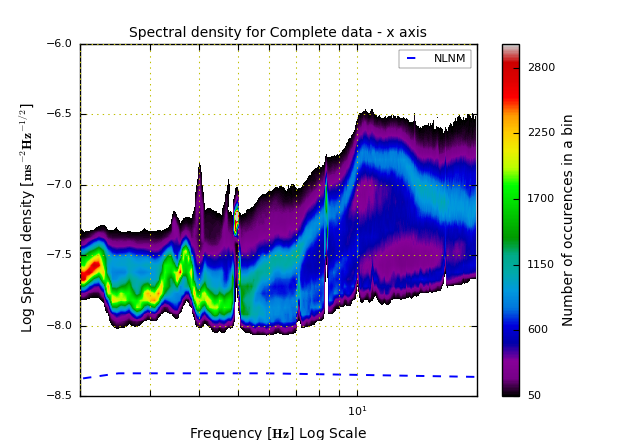
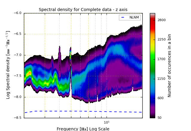
Figure 18. The density plots of the spectra in the vertical and horizontal directions. The blue dashed line is the NLNM.

4.5. Complete daily analysis:

In order to investigate several types of spectra during different working times of the day in more detail we generated the acceleration ASD for periods corresponding to the working shifts in the mine, 09:00-15:00 UTC and 20:00-02:00 UTC. The acceleration ASDs for these periods were then binned and plotted for each axis for the whole data set. We present these in the panels of Fig. 19 for the working, and in panels of Fig. 20 for the night periods, respectively, like in the case of ET1H station. These plots show less variation than the plots for the entire data set. The lack of characteristic bimodality at higher frequencies indicates lack of noisy periods at night. The working period shows additional lines, that are not visible at the night. The night spectra have very little variability less than 0.3 dex over the entire frequency band.

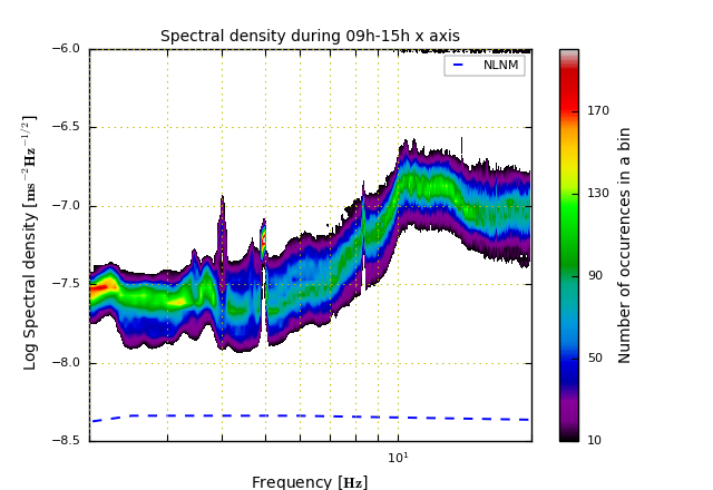
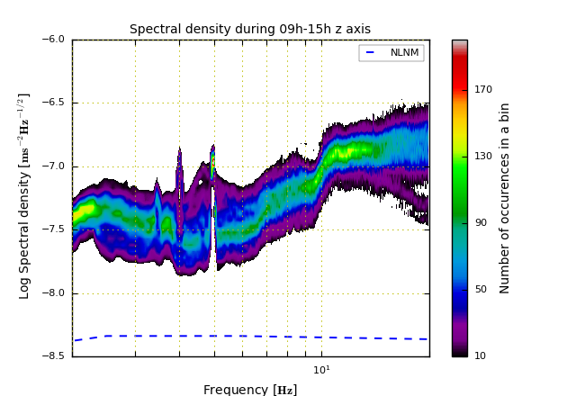
Figure 19. The daily variation of the seismic noise for the work-shifts in the mine: corresponding to the time between 09:00 and 15:00 hours UTC. The blue dashed line shows the NLNM curve.

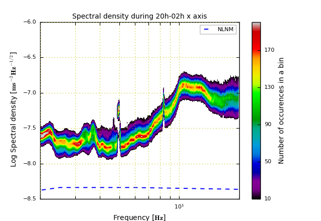
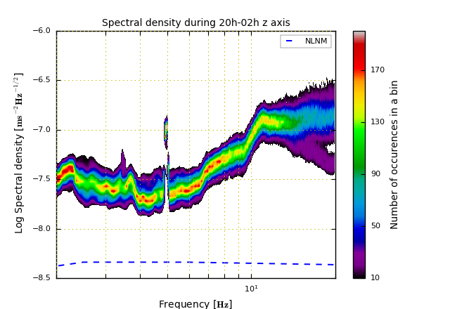
Figure 20. The daily variation of the seismic noise for the off work-shifts in the mine: corresponding to the time between 20:00 and 02:00 hours UTC. The blue dashed line is the NLNM.

4.6. Site parameterization

The values of $rms_{2Hz}$ were calculated for each hour of available data and the cumulative distribution function was plotted for the three axes of the detector in Fig. 21. The median $rms_{2Hz}$ $\approx 0.18$ nm in the vertical direction and $\approx 0.16$ nm in the horizontal directions. The two horizontal $rms_{2Hz}$ distributions are different below the median. It is unclear whether this is an instrumental effect or if this corresponds to the properties of the seismicity in MGGL.

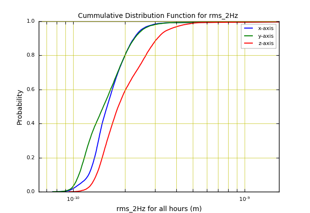
Figure 21. The cumulative distributions of the hourly $rms_{2Hz}$. We present the results for the three directions.

4.7. Conclusion:

In conclusion our measurements show that the seismic noise level is very low at the Mátra site. In spite of the spectral differences the median $rms_{2Hz}$ values are in agreement with the ET1H data of Table 5, measured by a different device.

5. An electromagnetic study on the signal attenuation in the ELF range

Since the gravitational wave interferometer’s mirrors of the proposed ET is going to be stabilized by means of magnetic fields, man-made and natural electromagnetic (EM) signals may also result in contaminated time windows of the gravitational wave observation. Magnetic noise from local sources can be identified based on correlation analysis utilising a network of extremely low frequency (ELF) field observatories. However, global EM components in the frequency range of interest may result in undesirable noise load [34]. The global thunderstorm activity exciting the Earth-ionosphere cavity continuously keeps a background signal at certain resonance frequencies called Schumann resonances [35]. Installation of the gravitational wave detector in a subsurface location may lead to lower EM noise even in the ELF range, $3-20Hz$.

An EM investigation has been carried out in close vicinity of the MGGL which aims to provide an estimation of the attenuation of EM signal with the depth in the Mátra andesite rock. ELF range geomagnetic observation stations has been installed at the backfilled end of a 140m deep cave and in the close vicinity of the surface projection of the subsurface measurement site. For technical reasons, the subsurface and surface recordings have been run with no overlap in time. Therefore an indirect processing method has been applied utilising the recordings of the very low-noise ELF EM observation site of Hylaty station as reference observation. The amplitude rate between the subsurface and the surface station has been estimated based on the experimental transfer functions between the subsurface-Hylaty and the surface-Hylaty relation.

5.1. The data acquisition system and the observation

The study is based on two mobile observations and an observatory data: time series from a subsurface site, a surface station and from a reference station. The subsurface measurement location could have been accessed from the town Mátraszentimre by an elevator crossing levels down to a tunnel at 140m depth. The observation site has been hundreds of meters away from the vertical mine of the elevator and from all active electronic facilities at that level. Notice that active loads have been in operation during the measurement in other levels of the mine, around 50m and 20m distance vertically. The subsurface data acquisition system consists of a Lemi-423 wide band magnetotelluric station and two Lemi-120 induction coils. The coils have not been fitted to a common plane to increase the separation distance to reduce the inductive coupling effect between the coils. The orientation of the coils have been set to the orientation of the tunnel: NNW-SSE and ENE-WSW, with NNW 22^∘ to North. The timing of the subsurface station has been initialised at the surface by means of GPS synchronisation and had been transported in the proposed site in operating status with no sensor connected. During the whole measurement session (Period I), the inside clock of the station has not been synchronized due to the lack of GPS or NTP access. The station was powered by a fully charged 84Ah battery. The data logger has been installed 40m away from the sensors along the tunnel. The connector of the coils and the whole instrumentation have been waterproof sealed, since high humidity and leaking water could lead to shortcut of the connector part. The sampling frequency has been set to 2kHz.

The surface measurement has been carried out after the subsurface measurement (Period II) and by means of the same Lemi station which has been set up at the subsurface site before. The coils have been buried 50cm deep in a common horizontal plane in perpendicular orientation. The separation of the sensors was more than 10 meters and the Lemi-423 station has been buried 40m away. The Lemi instruments and the wires have been buried preventing harmful activity of forest animals. The orientation of the coils at the surface stations has been set to NNE-SSW and WNW-ESE adapting to the local environment conditions. The sampling frequency has been set to 2kHz at this mobile station, too.

The Hylaty geophysical station was proved to be the optimal ELF observation facility as reference station based on data quality and geographic aspects too, [36]. The Hylaty station provides very low noise ELF geomagnetic data at around 888Hz sampling rate which is optimal for the proposed study as reference.

5.2. Data processing

5.2.1. Data preparation

The primary goal of the study is to provide an estimation of EM attenuation of the overlying andesite block in the lower ELF range, especially at the first Schumann resonance frequency. In the aspect of the measurement configuration it is identical to the relation of the absolute value of the empiric amplitude transfer functions of the subsurface and the surface stations at certain frequency. Since the surface and subsurface observation time periods were not overlapping the direct comparison of the amplitude spectra was not possible. The concept of the processing is based on utilization of a high-quality, low-noise ELF reference station data covering all the studied time intervals. The indirect method is basically as follows: determination of Tc_deep/ref power transfer coefficient in Period I. than the Tc_surface/ref in Period II and finally the estimation of the attenuation is accounted to the relation of the two coefficient. The amplitude attenuation has been derived as the square root of the power transfer coefficient of subsurface-surface site relation. The observations took 4 and 7 days in Period I. and II., respectively.

After resampling the three datasets to a common frequency of 800Hz both mobile data have been rotated in the coordinate system of the reference site. The magnetic components of the subsurface and the surface observation have been transformed by 22^∘ and 55^∘, respectively. Since the infrastructure of the mine has been operating during the whole observation campaign, the time and frequency domain identification of low magnetic noise intervals has formed the basis of the forthcoming processing. The variation of the x component in time and time-frequency domain is plotted in Fig. 22. An intermittent broadband load with maximum at 50Hz has been demonstrated for the whole observation period and besides of that a peak appears at around 15-17Hz, too for several minutes by no regular timing. These large power load periods are related to the operation phases of the elevator of the mine shaft and the latter one is originated by the horizontal transportation and the lighting on active levels of the mine. Both have been present in the whole observation period. The low-noise segments have been identified based on the dynamic magnetic spectra covering Period I. Finally the remaining subsurface data consists of thirty one 80-100 second long time series of relatively quiet time segments, selected for further processing. The low noise windows are concentrated in the early afternoon hours of 24 March, 2018, 12:00-16:00 UTC. For the reason of having similar relative position between the observation site and the source area the same temporal pattern of time segments have been selected in Period II from the surface magnetic variation time series on 13 April, 2018. From the reference data the same temporal pattern of time sections have been selected for the estimation of the transfer functions in Period I and Period II, too.

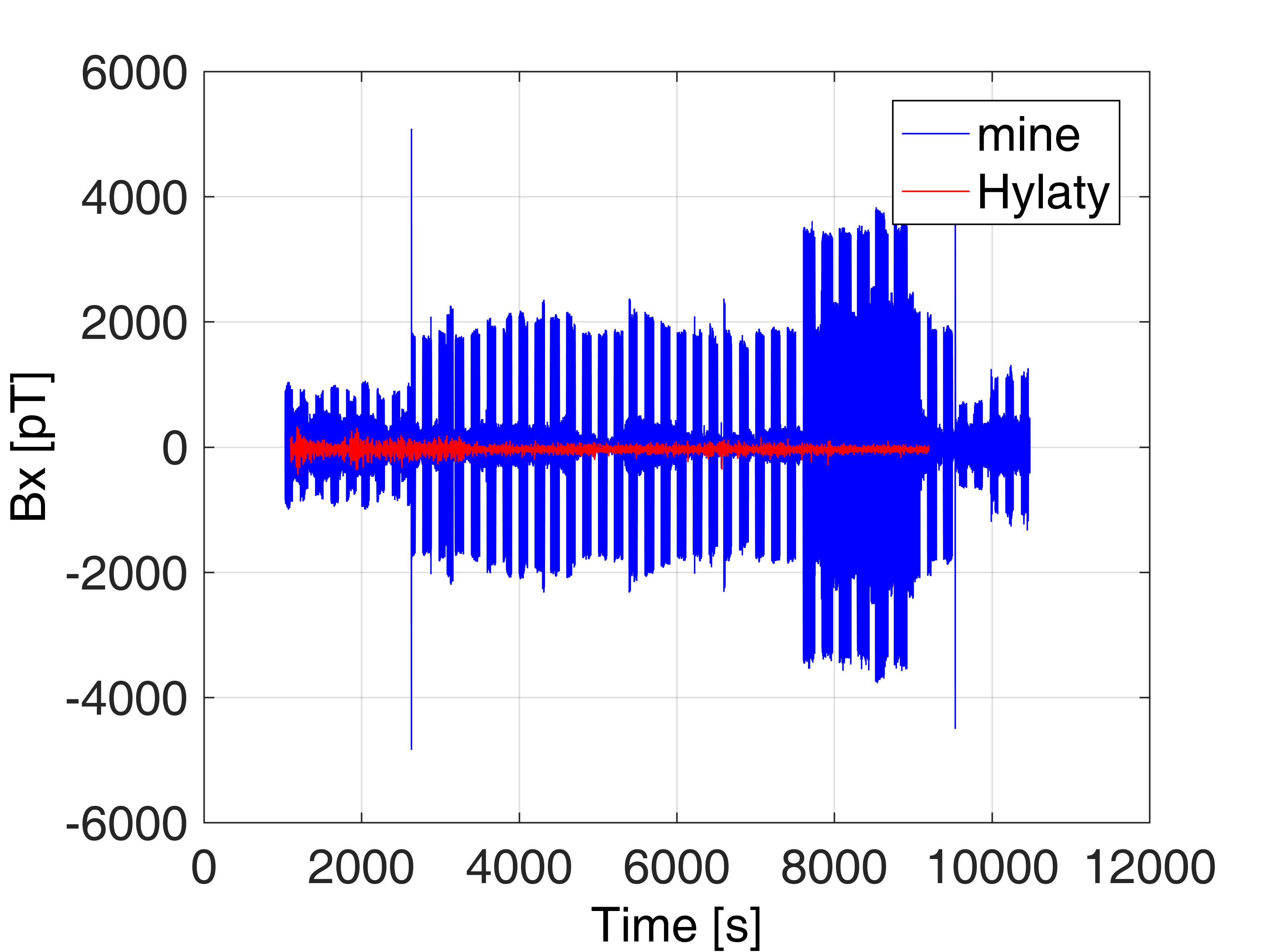
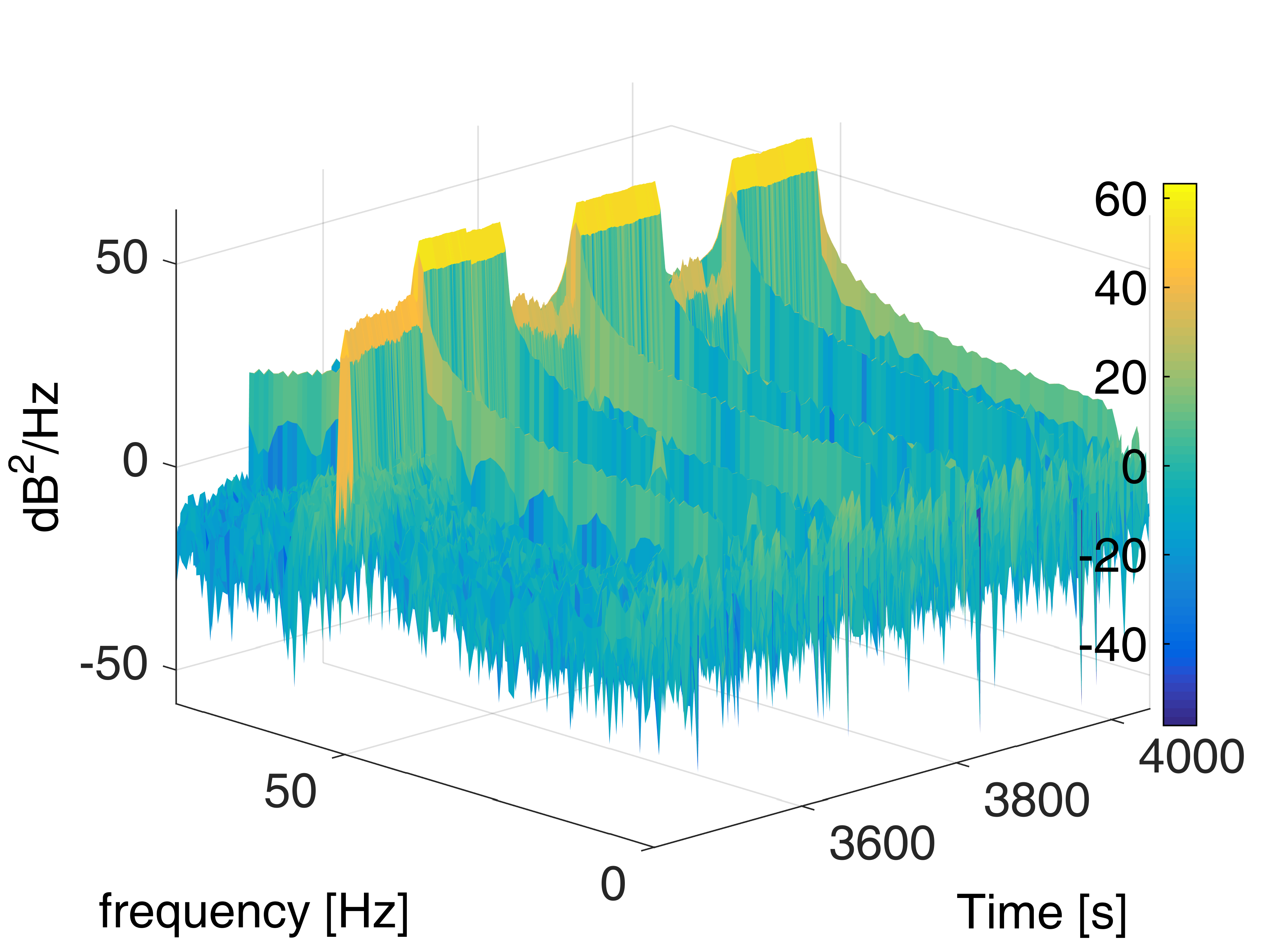
Figure 22. A ten minute long time series of subsurface registration (left). Blue lines are for N-S, red ones are for the corresponding section of the $x$ channel of the Hylaty reference station. A shorter section of the corresponding dynamic spectral power density of the magnetic variation at the subsurface observation site is plotted on the (right).

Since the inside clock of the data logger has a characteristic delay per day, post synchronization of the subsurface data have been applied first. The method is based on the comparison of the same natural signal recorded on both stations: cross correlation function of the subsurface and the Hylaty data have been estimated on the 31 pair of selected time series sections. Preparation of magnetic data sections by the application of a 5.6-25Hz bandpass Butterworth filter was necessary to attenuate the strong effect of the 50Hz peak of the power grid on the cross correlation function. The time delay according to the cross correlation was 4 samples which means 5ms for both channels. It has been corrected assuming linear drift of the inside clock time. The total magnetic time series has been correlated in both relation of the subsurface-Hylaty and surface-Hylaty observations. The cross correlation of the bandpass filtered total variations are overlay plotted for each section pairs in Fig. 23 after post synchronization. The cross correlated time sections contain minimum 64.000 samples each at 800Hz sampling rate. After the same processing, the cross correlation between surface registration and reference data has also been demonstrated, see Fig. 23.

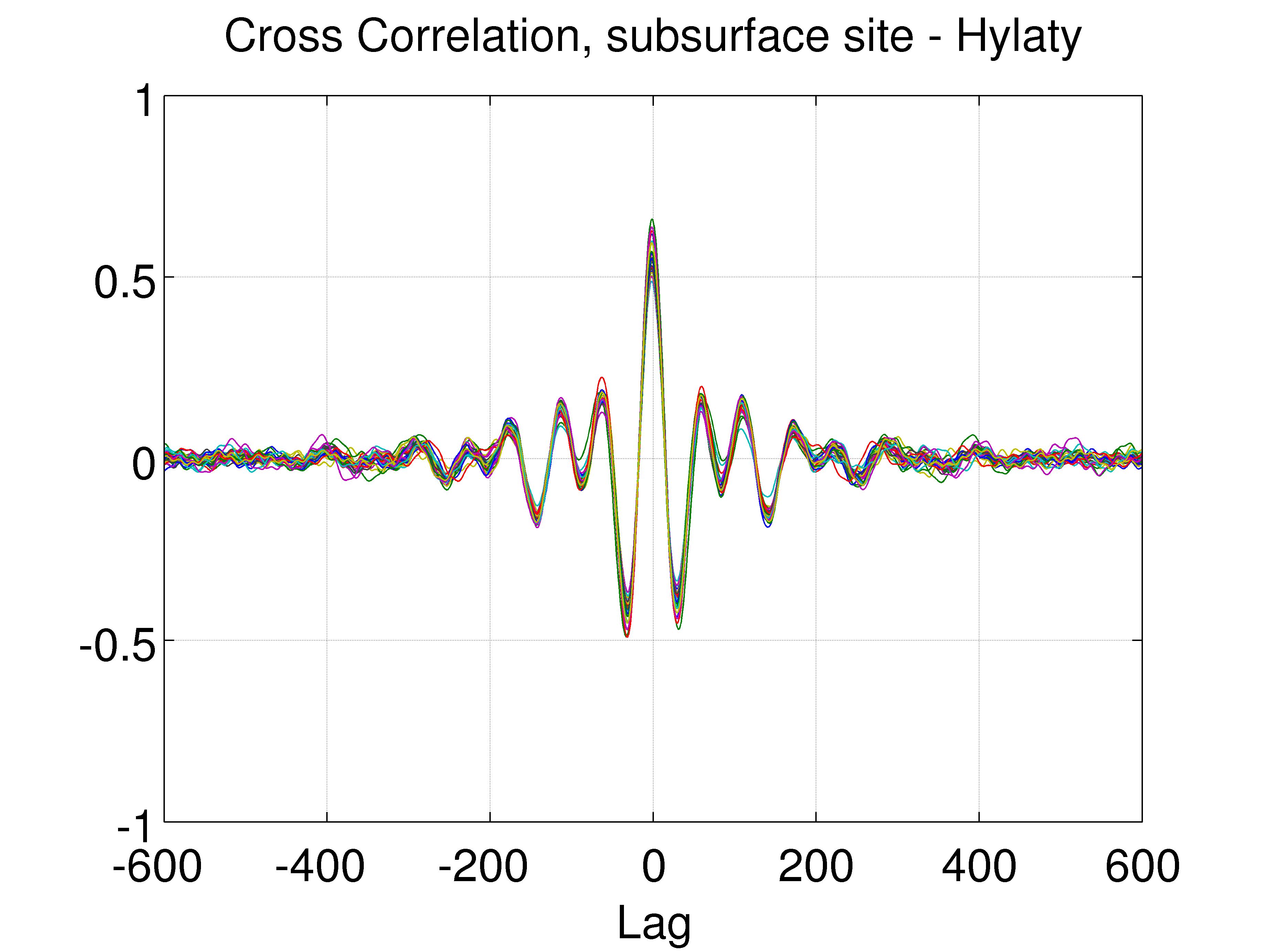
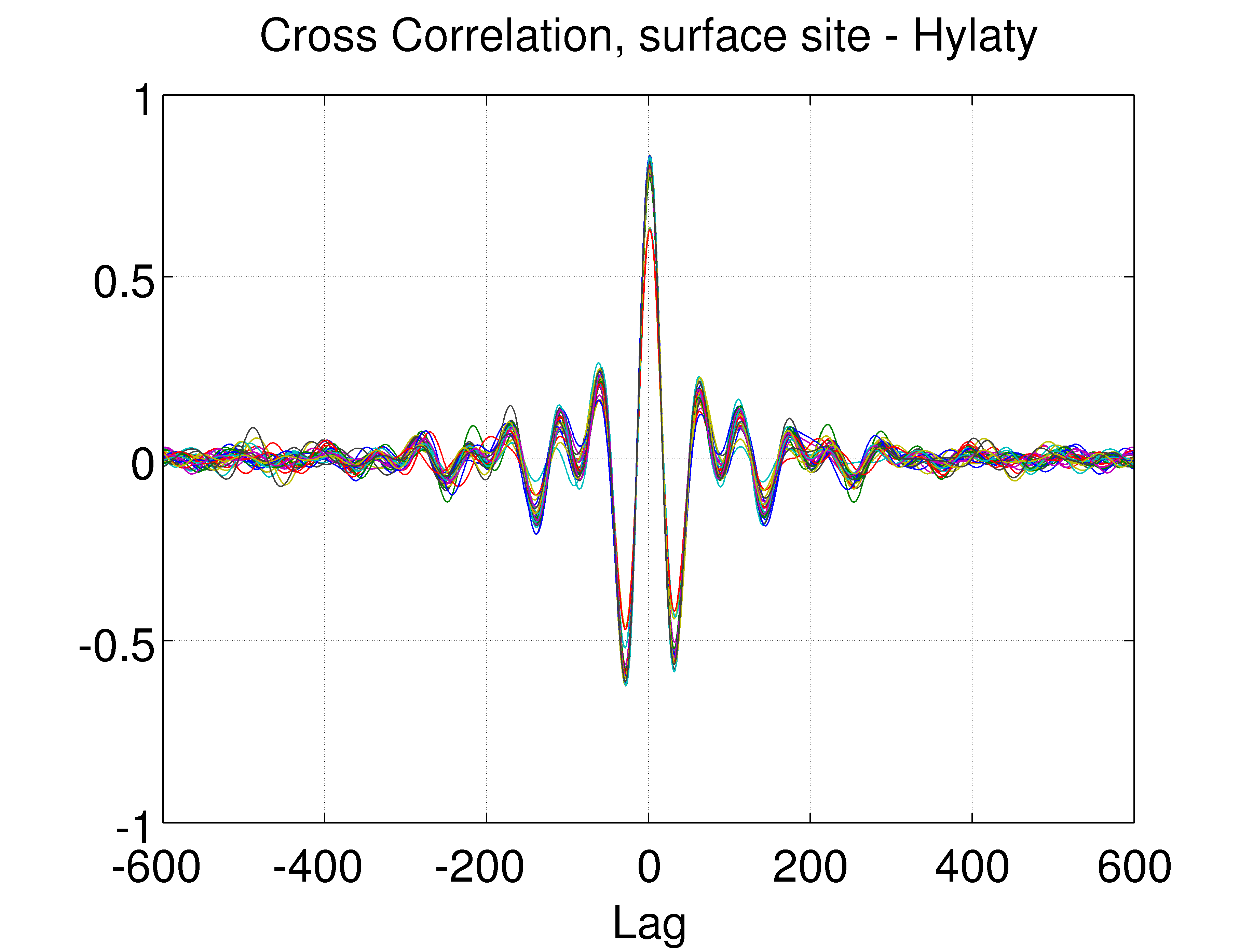
Figure 23. Cross correlation between the bandpass filtered total magnetic variations observed in the subsurface and at the Hylaty reference site (left). Each color corresponds to one selected quite time window of the 31. The high peak at zero demonstrates that the subsurface station observed the same natural signal as the Hylaty station in each time sections. In the Period II. cross correlation between the bandpass filtered surface and the reference data is on the (right). The plot confirms the correlation between surface observation and the reference observation in the frequency band of 5.6-25Hz for the same pattern of daily distribution of time segments in Period II.

The sharp and high peak at zero demonstrates that the subsurface station observed the same natural signal as the reference station. In frequency domain the correlated components have also been confirmed by computing the spectral coherence between the magnetic variations in relation of subsurface-Hylaty and surface-Hylaty datasets, see Fig. 24. The spectral coherence plots indicate definite correlation at the first three Schumann resonance frequencies in relation of both subsurface-Hylaty and surface-Hylaty site.

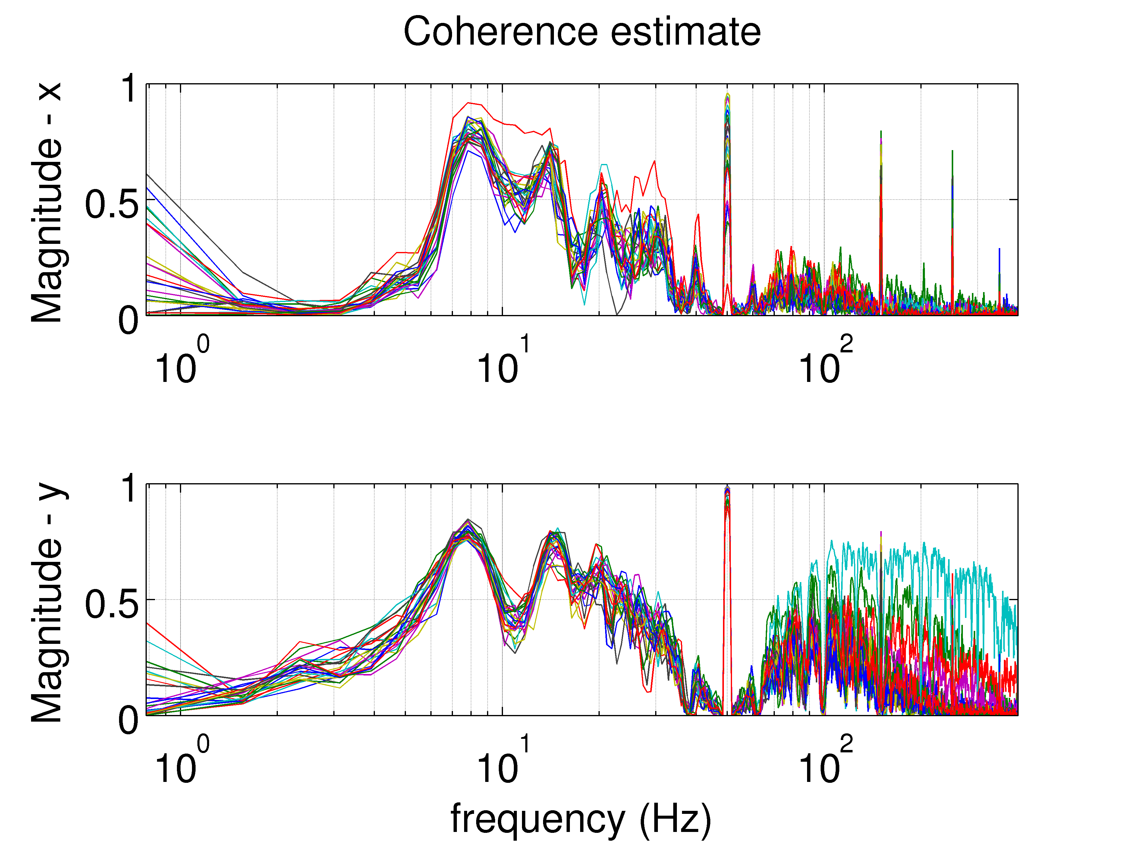
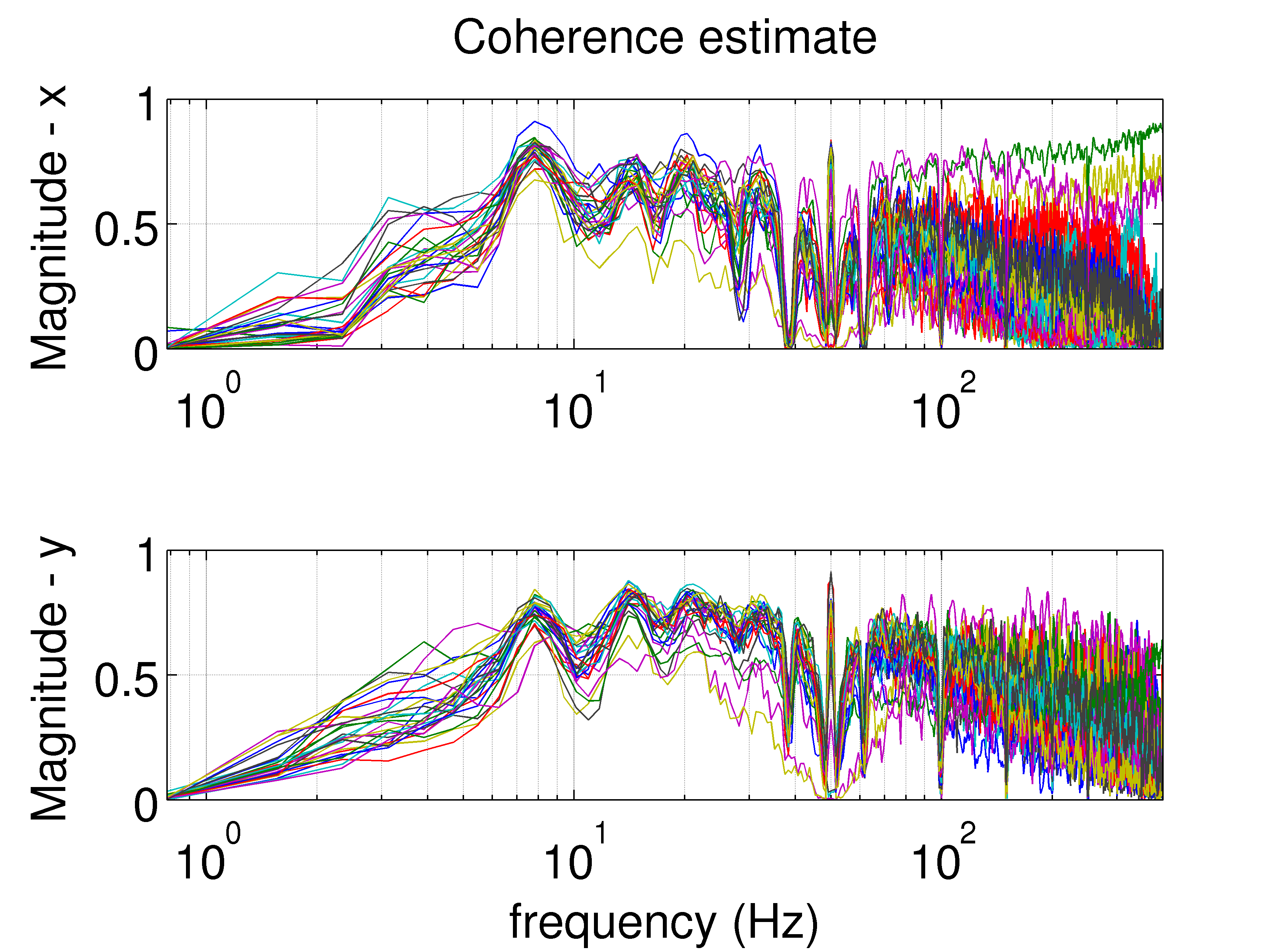
Figure 24. The coherence of magnetic variation in relation of both subsurface-Hylaty (left) and surface-Hylaty site (right) indicates definite correlation at the first three Schumann frequencies.

Finally, four dataset has been prepared for the estimation of the transfer functions of subsurface-Hylaty and surface-Hylaty relation and finally to the determination of the surface-subsurface transformation:

1. $B_{I.mine}$: 31 selected time segments in Period I, subsurface magnetic variation;

2. $B_{I.Hylaty}$: the same 31 time segments in Period I, reference site magnetic variation;

3. $B_{II.surface}$: 31 selected time segments in Period II with the same daily distribution, surface site magnetic variation;

4. $B_{II.Hylaty}$: the same 31 time segments in Period II, reference site magnetic variation;

5.3. Results

The introduced processing steps resulted in four dataset, which are accurately synchronised, transformed to the same coordinate system and resampled to a common sampling rate of 800Hz. The data has been prepared for time domain and spectral analysis. Additionally it has been confirmed that the subsurface observation and the Hylaty reference station has observed the same natural signal which variation is considered to be homogeneous in the scale of their relative distance,  300km. It has been demonstrated in the surface-Hylaty observation, too. The analysis of the distribution of the spectral power values at individual frequencies demonstrated non-normal distribution of the spectral power. The mean, the median and the interquartile range (IQR) of the spectral power have been plotted in Fig. 25.

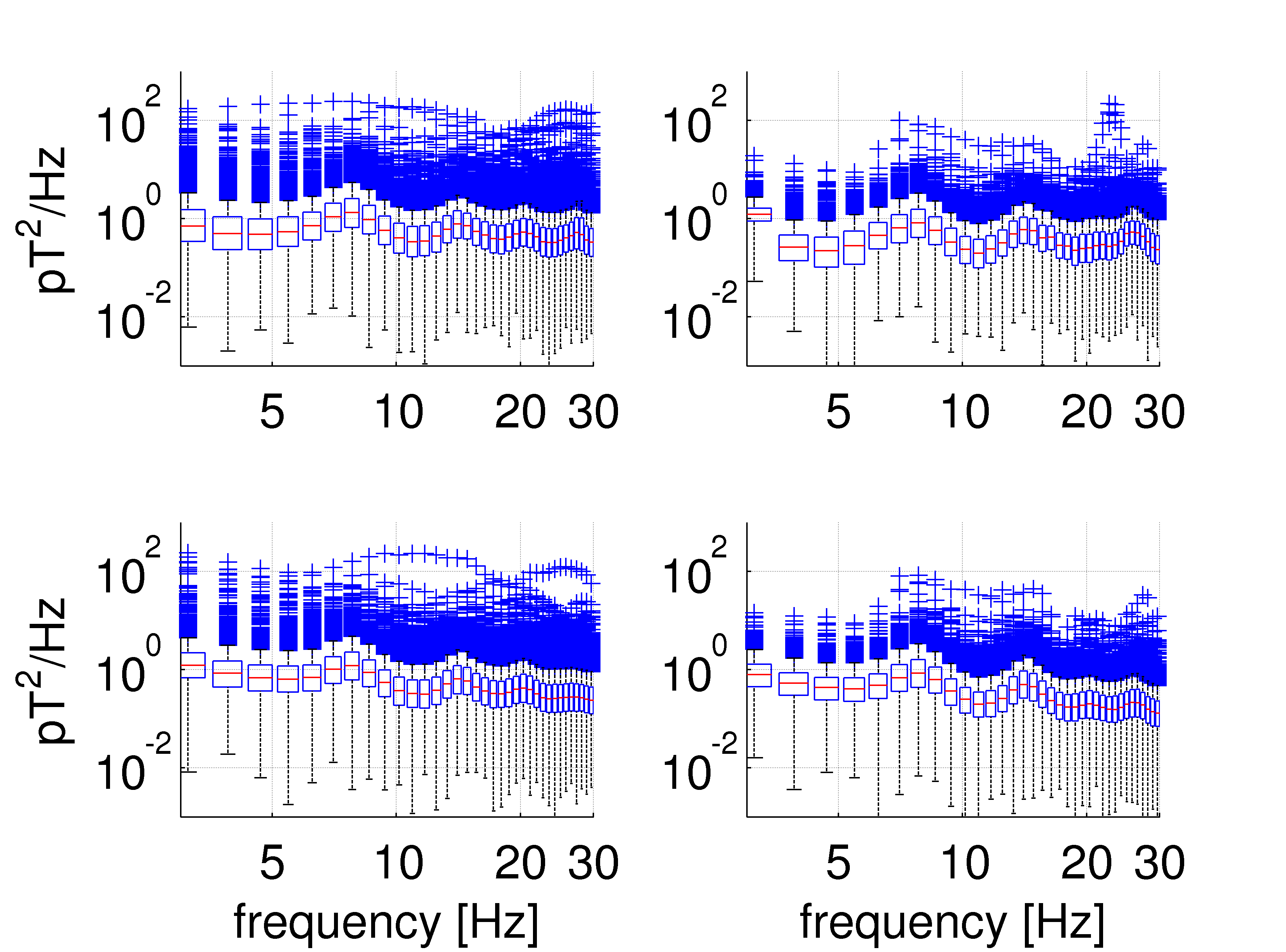
Figure 25. The median, the interquartile range and the outliers of power spectra are plotted in relation of the four observations, (subsurface data: upper, left; Hylaty data - Period I: lower, left; surface data: upper, right; Hylaty data - Period II: lower, right). The red line in the middle of the boxes represents the median, the blue box is for the interquartile range, the black bar is for the range of the most extreme data samples not considered outliers and the blue crosses represent the outliers.

In the first approach no outlier removal algorithm has been utilised, but the simplest robust statistics, the median of the spectral power has been determined at each frequency values. For the estimation of the signal attenuation with the depth, the median of the power spectral density (PSD) has been computed related to the four datasets, $B_{I.mine}$, $B_{I.Hylaty}$, $B_{II.surface}$ and $B_{II.Hylaty}$. The four PSDs have been plotted in Fig. 26.

Figure 26. Median of power spectral density of the EM noise of the four dataset: observation at the subsurface site in Period I., observation at the reference site in Period I., observation at the surface site at Period II. and at the reference site in Period II., respectively.

All four median PSD functions have been determined from the Fourier transform of 1024 sample long consecutive time windows, with 512 sample overlapping between adjoining segments, using Hamming window. For an estimation of the power attenuation with the depth, the power of the fundamental Schumann spectral component has been determined in case of all four observations. The following subsection introduces a method which has been applied to have accurate estimation of the fundamental Schumann resonance spectral power peaks related to the four observations.

5.3.1. Polynomial baseline approximation

The method to provide an estimation of the ELF range attenuation is based on utilisation of an advanced background baseline removal technique. In this method the baseline is estimated by fitting a low-order polynomial, but instead of obtaining parameters by minimising the sum of squares of the residuals a non-quadratic cost function is adapted [37]. Third order polynomials have been considered to fit the median PSDs in a limited frequency range, see left four subplots of Fig. 27. All polynomials have been fitted by means of asymmetric truncated quadratic cost function.

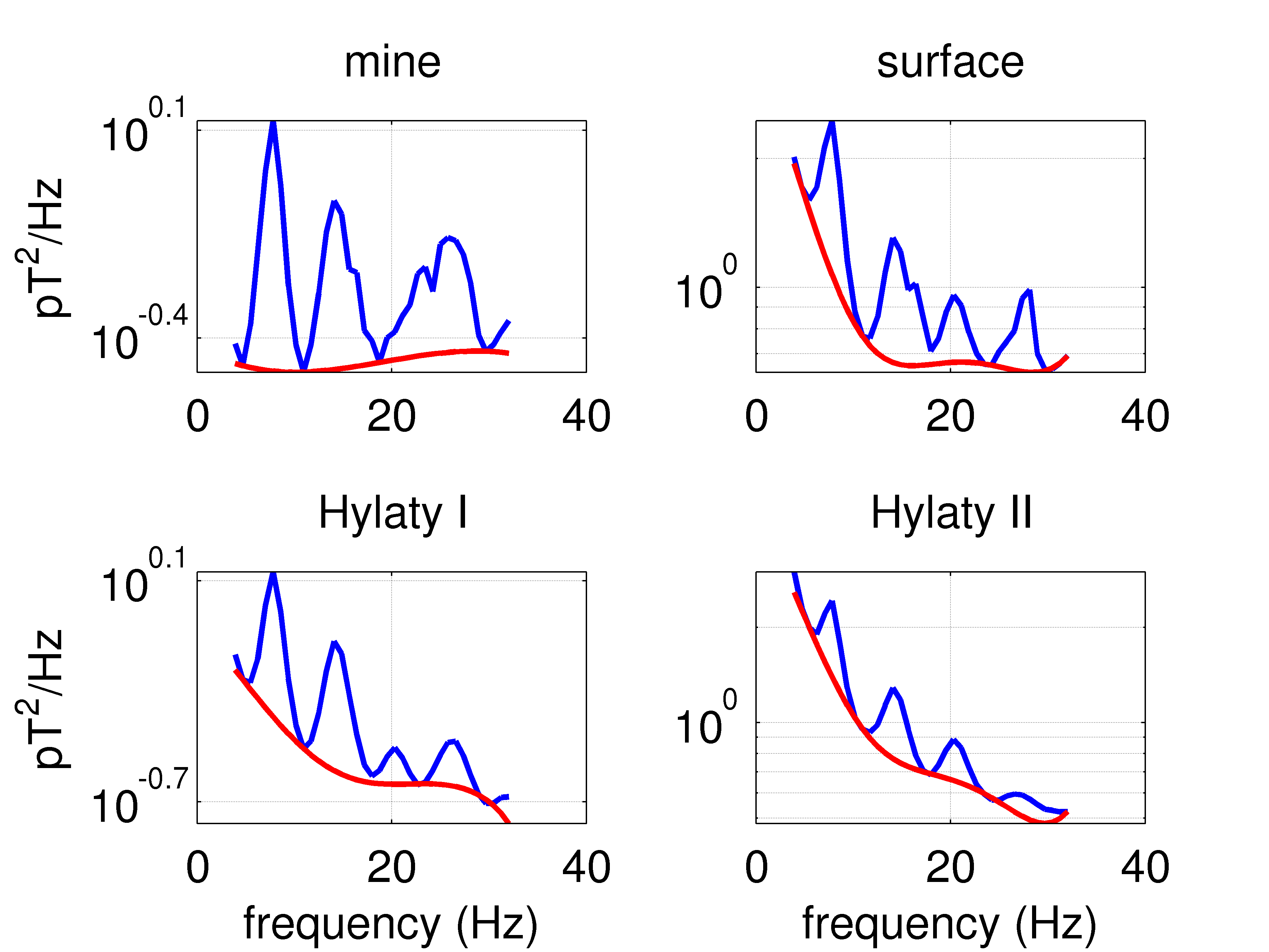
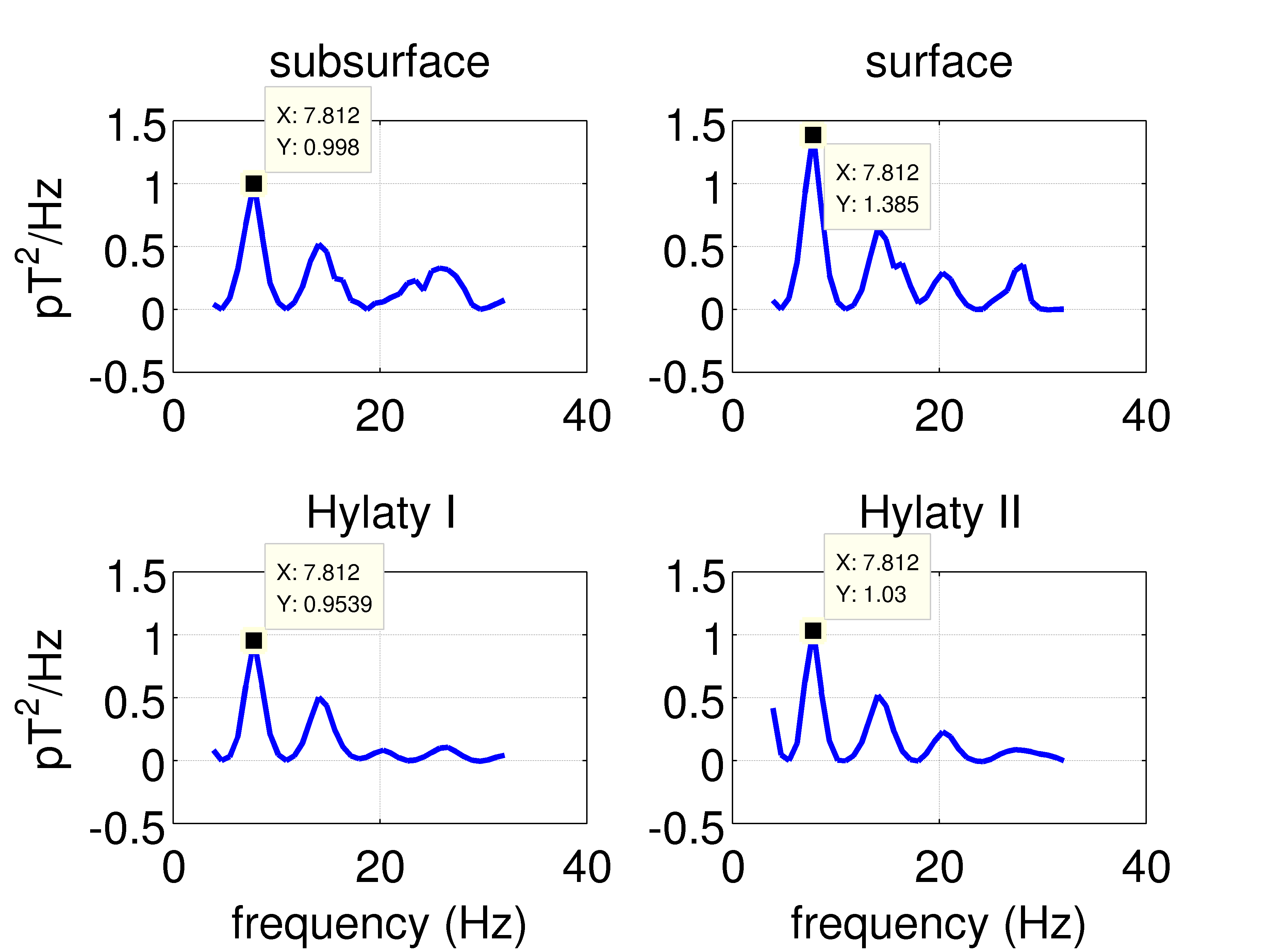
Figure 27. Polynomial baseline fitting on median PSD of the four dataset (left) and median PSDs after baseline removal (right).

The fitted baseline polynomials have been substracted from the power spectra, plotted on the right four subplots in Fig. 27. The power ratio obtained at 7.81 Hz in the subsurface-Hylaty relation is 1.126, for the surface-Hylaty relation 1.219 which results a power ratio of 0.924. The square root of the power ratio results the estimated amplitude attenuation: 96.1%. The rate of signal amplitude between the surface and at depth h can generally be computed by writing the exponential decay of the magnetic signal amplitude as follows:

$$\frac{A(h)}{A(0)}=\exp(-h/\delta)$$ (9)

By substitution of the empiric amplitude rate values and the 140m depth of the subsurface station the characteristic depth of the amplitude attenuation, the so called the $\delta$ skin-depth can be estimated. It results $\delta=3520$ m. The power decrease of the signal with the depth is a consequence of the nonzero electrical conductance of the underlying/overhead andesite rock. Providing an estimation of the bulk resistivity of the andesite block is possible by a simplified approach of homogenious half space approximation. This estimation is considered valid if the homogenious halfspace assumption is realistic. A simple approximation formula between the skin-depth and the bulk electrical resistivity is as follows [38]:

$$\delta=500\,\sqrt{\rho\times T}.$$ (10)

Extracting the bulk resistivity by substitution of estimated skin-depth value of the Schumann fundamental resonance frequency 387 $\Omega$m is obtained. The estimated resistivity value is in the wide characteristic range of electrical resistivity of the andesite rock in the literature (170-45.000$\Omega$m)[39].

5.3.2. Time domain investigation

A recent electromagnetic study of ELF range magnetic signal attenuation could have been explained by the assumption of distortion effect of iron artifacts of the mine infrastructure. For this reason the time domain inspection of the bandpass filtered subsurface data has been carried out. Bandpass filter is tuned below common power grid frequency and below upper Schumann frequencies to have comparable pattern of the hodographs. Based on this, 5.6, 10Hz cut off frequencies has been set. About 100 sample long time windows have been picked from the subsurface data and the corresponding reference time series. The magnetic variation of a time segments has been plotted and compared in Fig. 28.

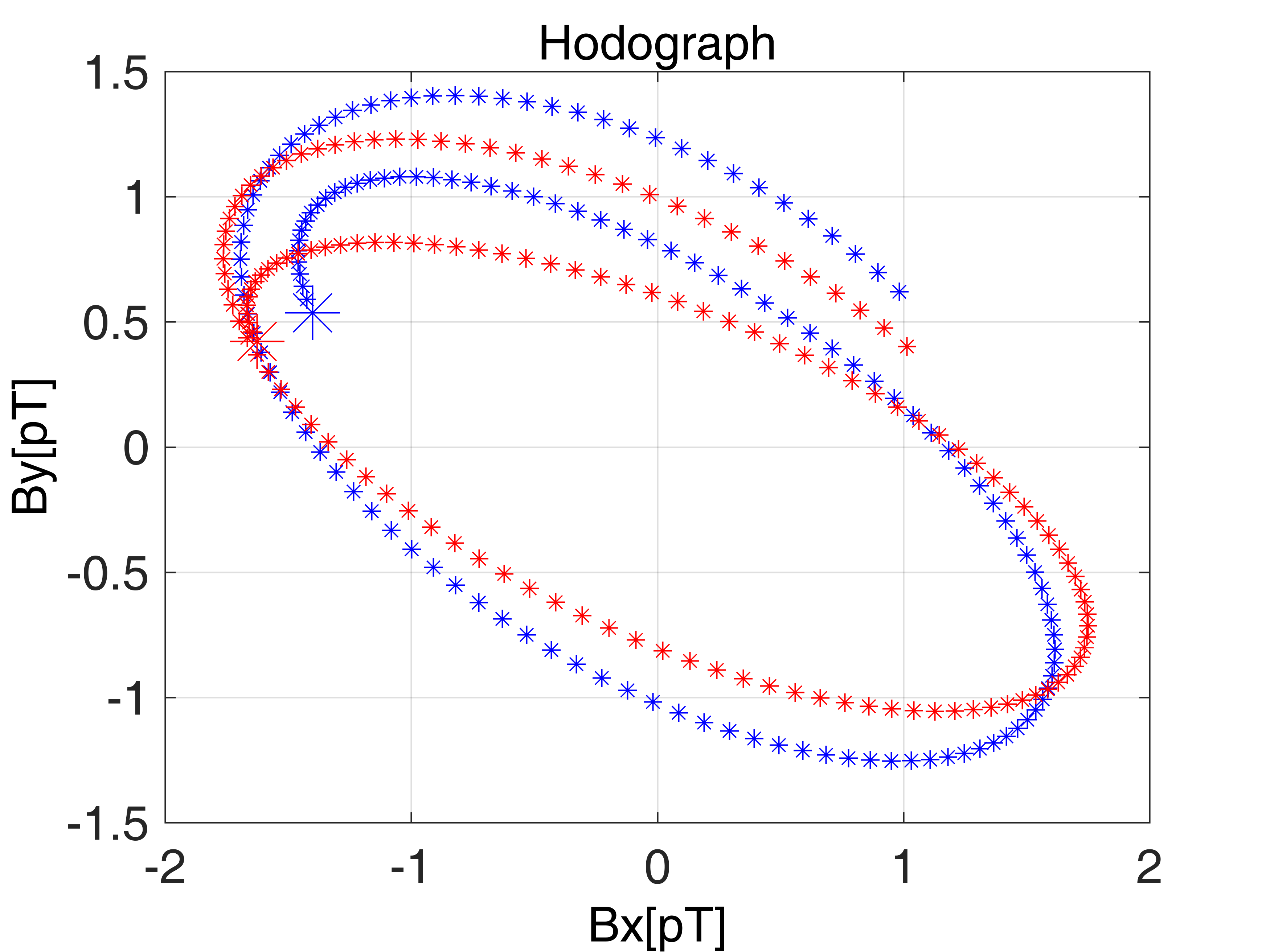
Figure 28. Hodograph of a randomly chosen segment of subsurface (blue) and the corresponding reference observation window (red) stars respectively.

The hodograph demonstrates no strong deviation of the subsurface signal is present confirming that iron parts of the mine infrastructure did not have recognizable effect on the subsurface observation and the estimated attenuation rate at the subsurface measurement site. The noisy environment, the amount of data utilised and the indirect comparation of the signal transformation all increase the deviation of the results and the variance of the power spectra. Considering all these circumstances the obtained attenuation value confirmes that in less noisy intervals, parallel measurement of surface and subsurface relation together can significantly improve the quality of the data and may provide more accurate estimation of the amplitude attenuation in the ELF range. Application of outlier removal may result further improvement on the quality of the estimation, too. The main goal of the study was to provide an estimation of the magnetic signal attenuation with depth. The results confirm that even an indirect estimation method can be promising. The estimation of the attenuation coefficient of the overhead andesite block might be more accurate by means of the data observed in an upcoming EM silent time window and even the more with the possibility of parallel recordings at the surface and subsurface sites. These two circumstances should improve the accuracy of the estimation significantly.

6. Infrasound measurements

6.1. Introduction

Sensitivity of second generation gavitational-wave detectors at low frequencies are limited fundamentally by the thermal noise of the suspension last stage and of the test masses, the seismic noise, and the gravitational gradient noise (so-called Newtonian noise (NN) ) resulted by changes in density of medium near the detector. Seismicity is one source of this type of noise, but changes in density of air caused by pressure waves are also contribute to NN [40].

Inspired by recent theoretical investigations of NN from the infrasound below the Earth surface [40], we have continued our infrasound measurements in MGGL. For these measurements, new infrasound microphone (ISM) was developed by the Institute for Nuclear Research of Hungarian Academy of Sciences (Atomki) [10]. The first instrument was installed at MGGL in 2016 with the purpose on one hand to test its performance on the long-term, and on the other hand to characterize the underground site’s ambient infrasound noise.

In this study, Bowman’s low- and median noise models were used as a reference for our site characterization. According to Ref. [41], the main sources of infrasound noise on the surface of Earth are microbaroms and the wind. These sources are not present underneath, but other sources related to the miner’s work and machines produce infrasound. Our results show that ambient infrasound presumably can be supressed when going under the ground, but the local noise sources and the geometry of the underground site influences the possible extent of the noise supression at different frequencies.

6.2. The instrument

ISM consist of two main parts: an industrially manufactured capacitive sensor and C-V converter, developed by Atomki. The capacitive sensor is a differential pressure sensor with two inlets. One inlet is connected to the environment, while the other is connected to a reference volume. A diaphragm is placed in between the two pressure inlets. The diaphragm is deflected when the difference between the environment and the background pressure changes. The deflection is converted into an electrical signal by the sensor, then the signal is amplified to the $-10-10$ V range. There is a leak with a diameter of $250$ microns, which connects the background volume to the environment. It makes possible to slowly equalize the background pressure and the environmental pressure, and hence determines the lowest frequency of the measuring range. The main characteristics of two versions of ISM are given in Table 11.

	ISM1	ISM2
Input voltage (V)	6-10	7.5-12
Output volt. (V)	0-5	-10-10
Sensitivity (V/Pa)	0.2	1
Pressure range (Pa)	-12.5-12.5	-10-10
Frequency range (Hz)	0.01-10	0.01-10
Temperature sensor	yes	yes
Humidity sensor	yes	no

Table 11. The characteristics of the two infrasound sensors, ISM1 and ISM2, developed in ATOMKI.

The drawback of the structure of the instrument is that fast changes in temperature $dT/dt>2\ ^{\circ}$C/h introduce artifacts in spectrum below 1 Hz. When the frequency of the temperature changes is in the measuring range of the detectors, then the temperature change initiated pressure in the background volume cannot be distinguished from the pressure change due to environmental infrasound. Therefore a high-resolution temperature sensor is built into the detector.

6.3. Data acquisition system and data processing

The microphones have analog output. In order to sample, digitalize and store measurement data, a low-cost data acquisition system is added to the sensors, based on a Raspberry Pi 3 model B [10].

The spectral properties of the infrasound background are characterised by the Pressure Amplitude Spectral Density ($PASD$) and the analysis of the data is similar to the seismological noise evaluation in Section 3. The collected data was downsampled to $100$ Hz, then divided into $163.84$ s long segments. For each segment, PASD was computed. For each day, the $5\textsuperscript{th}$, $50\textsuperscript{th}$ and $95\textsuperscript{th}$ percentile of corresponding PASD data was determined.

6.4. Comparative measurements with MB3 microbarometer

In order to compare performance of ISM1 with the performance of MB3 microbarometers [42], comparative measurements were performed on 2018-04-26 at Infrasound station no. 3 of Piszkéstető observatory in Mátra mountain range, Hungary. This station is part of the Hungarian National Infrasound Network, which is a permanent infrasound network operated by the Kövesligethy Radó Seismological Observatory of the Hungarian Academy of Sciences [43].

At Piszkéstető, the MB3 microbarometers are placed in a reservoir, which is partly covered by soil. MB3 is equipped with a wind reducing system of long pipes attached to the microbarometer. During our measurements, the pipes were detached, and the MB3 and ISM1 were placed next to each other in order to detect similar pressure as much as it is possible. The measurement lasted for three hours.

Our aim was to calibrate our instrument, that is to determine the real PASD values in Pa/$\sqrt{Hz}$ from the PASD_ISM1 given in $ADCunits/\sqrt{Hz}$ computed from measurement data. During the data processing part, raw signals both of MB3 and ISM1 were cut into $128$ seconds length segments and PASD_MB3 and PASD_ISM1 of each segment was computed. Then values corresponding to a given frequency of PASD_MB3 and PASD_ISM1 pairs from the same time interval were collected. The number of pairs corresponding to a given frequency is equal to the number of segments used for calibration. For a given frequency, the ratios of PASD_MB3 values and PASD_ISM1 values were computed (C=PASD_MB3/PASD_ISM1). The distribution of these ratios corresponding to a given frequency can be approximated with normal distribution. Standard deviation ($\sigma_{C}$) of the distribution was estimated by using median absolute deviation ([44]). Two standard deviations were chosen to express the uncertainty of the ratio in Fig. 29.

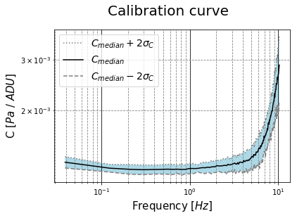
Figure 29. Calibration curve used to convert PASD given in $ADCunits/\sqrt{Hz}$ of ISM1 to PASD in $Pa/\sqrt{Hz}$.

6.5. Ambient infrasound noise at MGGL

This study shows the results of a two-week long period of measurements that started at 2017-06-01. This is the period of the deep seismic noise measurement campaign, when the ET1H seismometer in MGGL at $-88$ m worked parallel with GU02 seismometer at $-404$ m in the mine. The colored area shows the interval between the 5^th and 95^th percentiles in Fig. 30. One can see, that the noise at MGGL roughly falls between Bowman’s low-noise and high-noise curves. The particular shape of the PASD bar on Fig. 30 may be resulted by the geometry of the tunnels in the mine and the other circumstances related to the ongoing reclamation (e.g. sound from machines). The size of laboratory itself allow resonances with higher frequencies, out of the infrasound range. Median noise of MGGL falls below Bowman’s median-noise curve only below $0.4$ Hz and above $5$ Hz, and newer falls below the low-noise curve. These results are showing that machinery and other activities at an underground site have to be minimized in order to take advantages of installing gravitational detectors under the ground.

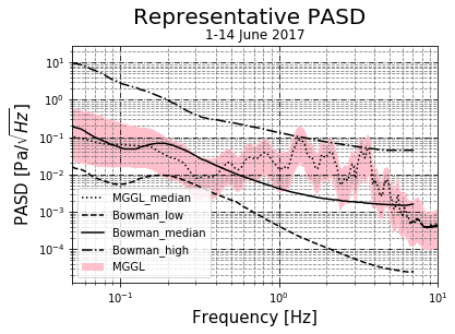
Figure 30. The pressure amplitude spectral density (PASD) of the ISM1 infrasound detector in the period 2017-06-01 – 2017-06-14. The dashed and solid black lines are the Bowman low noise and median curves.

6.6. Relationship between seismic and infrasound noise in the MGGL

In order to examine the relation between the signal of the seismometer and the signal of ISM1, we have computed the magnitude squared coherence estimate for each 128 s long data segment pairs from the deep measurement campaign of MGGL by using Welch’s method [45]. In the case of the ET1H seismometer’s signal, we treated the tree directions, East, North and Z (vertical) separately. This way, we got three datasets for the coherence: $C_{v_{E}p}$, $C_{v_{N}p}$ and $C_{v_{Z}p}$. We determined the average of the coherence values of each frequency of the three datasets. A peak between 3 and 4 Hz can be observed on each plot on Fig. 31, which indicates a common source has an effect both on the seismometer and ISM1. There were no similar coherences with the farther, GU02 seismometer. The drainage system or the ventilation system may be responsible for the peak. We will prove or refute this hypothesis with the forthcoming experiments in MGGL.

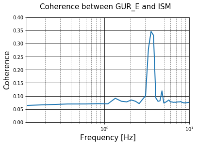
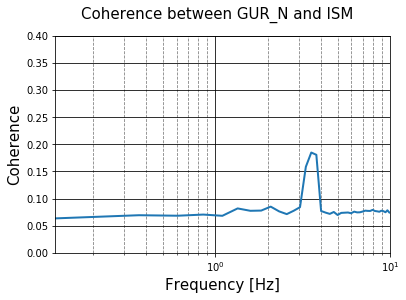
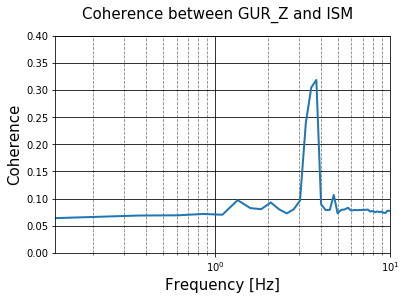
Figure 31. Average coherence between the three components (E: East, N: North, Z: vertical) of the seismic signal and the infrasound signal.

7. Measurements of the inhomogeneity and the rock-density at large-scale with cosmic muon tracking

A novel cosmic muon tomography technology were used to explore the precise, large-scale density structure of the Mátra mountain above the MGGL within the Gyöngyösoroszi mine. The idea is to measure the angular distribution of the highly penetrating muon-component flux of the cosmic-rays, which are created in the upper atmosphere and reach the surface of the Earth. This technique, has been applied successfully by our group for various cases such as cave researches, cosmic background measurements for underground laboratories, civil engineering, and volcano muography [47, 48, 49, 50, 51, 52].

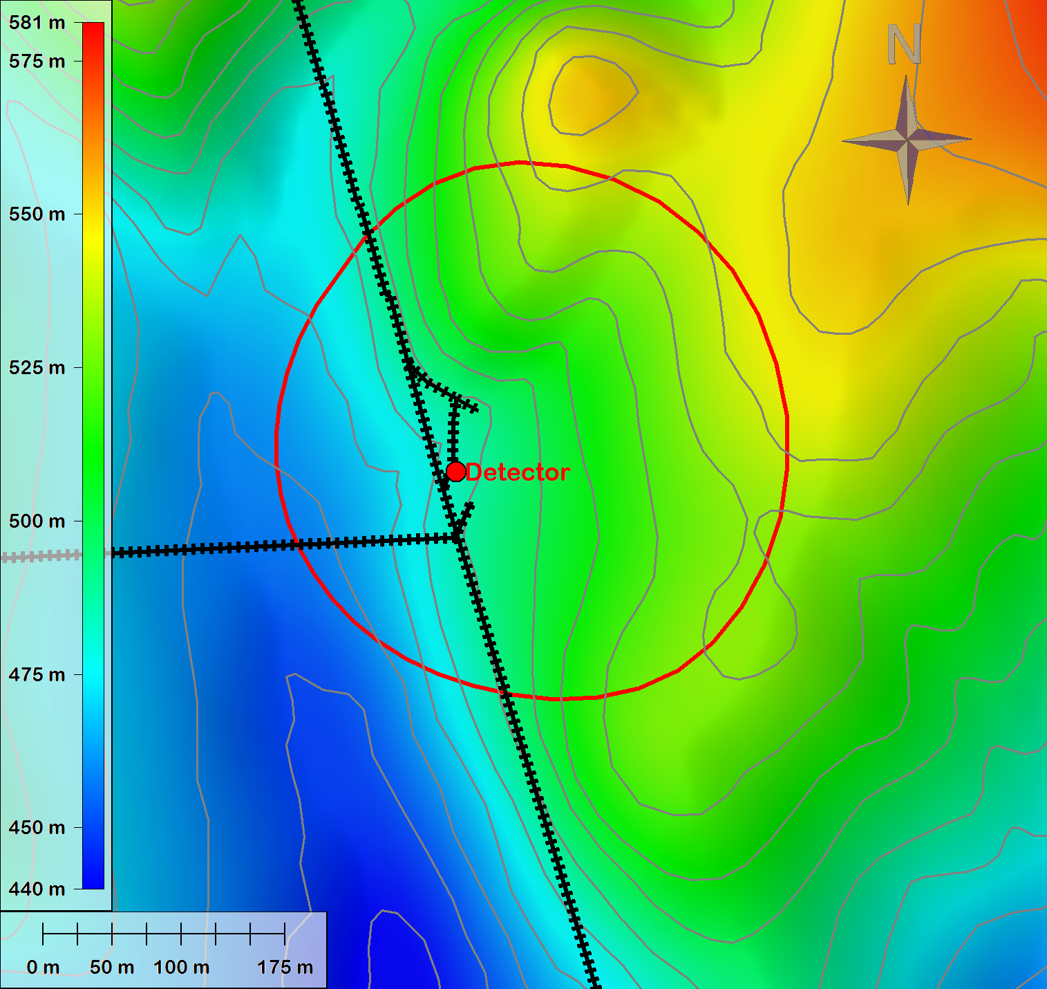
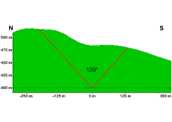
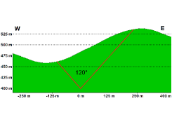
Figure 32. Left: the position of the MGGL Laboratory in the Mátra Mountain and the acceptance of the mun-flux detector with $60^{\circ}$ zenith angle. Color-scale contours and dark contures show the elevation in m.a.s.l. Right: West-East and North-South cross-sections of the Mátra Mountain at the MGGL and the acceptance of the mun-flux detector with $60^{\circ}$ zenith angle.

To reach the full, 2$\pi$ coverage, muon flux measurements were continued, using a portable tracking system, called the Muontomograph. This has been developed by the Wigner Research Centre for Physics and described in details in Ref. [10]. Based on the Run-0 experiences, we made modifications on the Muontomograph in order to get better performance in the MGGL laboratory for the Run-1. The position of the MGGL and the acceptance directions of the detector related to the surface topology are shown in Fig. 32. We adjusted the trigger levels for higher efficiency and a noisy chamber were also removed, thus the number of chambers were reduced to five.

7.1. Cosmic muon flux measurements in MGGL

During Run-1 the cosmic muon flux measurements were also continued in the Gyöngyösoroszi mine. The Muontomograph was located at the Northwest corner of the laboratory room at a depth of 88 m. We used the same position in the MGGL, where the detector were placed earlier in the Run-0 period. The duration of Run-1 was all together 280.0 days in four compass courses. Jointly with the 124.7 days of Run-0 measurements we have 404.7 days of data taking so far.

Since we have covered the zenith- and two 90^∘-tilted directions in Run-0, the four Run-1 measurements were all tilted to 45^∘ from the zenith. With this choice we could cover the upper hemisphere fully, without any missing direction. The first measurement was directed to 20.5^∘ for 77 days, then we continued to 110.5^∘, 200.5^∘, and 290.5^∘ directions, respectively for 62 days, 77 days, and 64 days. Further details of the measurements are summarized in Table 12. Data were monitored and downloaded continuously from the detector via Ethernet connection during the data taking period in MGGL for online checking of data quality.

Table 12. The summary table of the Run-0 and Run-1 measurements in MGGL: the detector principal direction in azimuth to the magnetic North and the tilt in zenith, the duration of the measurements, number of events, and the number of measured muon tracks.

Runs	Azimuth	Zenith	Duration (days)	Events	Num. of tracks
Run-0-M2	zenith	$0^{\circ}$	48.3	4.7 M	111,700
Run-0-M3	ENE$(65.5^{\circ})$	$90^{\circ}$	41.9	2.4 M	18,124
Run-0-M4	NNW$(335.5^{\circ})$	$90^{\circ}$	34.5	3.1 M	12,356
Run-1-M61	NNE$(20.5^{\circ})$	$45^{\circ}$	77.0	423.3 k	49,827
Run-1-M62	ESE$(110.5^{\circ})$	$45^{\circ}$	62.0	366.9 k	35,534
Run-1-M63	SSW$(200.5^{\circ})$	$45^{\circ}$	77.0	367.4 k	42,414
Run-1-M64	WNW$(290.5^{\circ})$	$45^{\circ}$	64.0	316.0 k	70,099

Comparing Run-0 and Run-1 date in Table 12, one can see that, although the event number dropped by an order of magnitude, the fraction of the track number increased relatively to the number of events. This means, that the efficiency become better since noise and fake events were suppressed well in Run-1.

7.2. Results of the rock inhomogeneity measurements

The muon flux distribution can be obtained after applying a track reconstruction algorithm and merging the maps according to the partial overlap and geometry normalization [51]. The Run-0 and Run-1 flux maps are shown in the left and right panels of Fig. 33 respectively. The muon flux distribution is plotted by color-scale contours as a function of azimuth and zenith angles.

The cosmic muon (track) rate was 0.005-0.02 Hz for both runs, which is sufficient to provide flux measurement with $5-50\%$ statistical errors (depending on zenith angle). The measured flux has a maximum value of 0.7 m^-2sr^-1s^-1 at $15^{\circ}$ zenith angle to the West. In Fig. 33 white color ’triangles’ at $20^{\circ}$ zenith angle (panel left) and ’dial’ at zenith (panel right) represents the directions, which are out of the acceptance of the current run.

The detector-to-surface distance is indicated with dark contour lines in the Fig. 33. For Run-0 in [10], we used Shuttle Radar Topography Mission (SRTM) satellite data for the elevation map with an estimated relative error of 10% (10 m at the zenith). However by comparing the SRTM model with other available elevation data the accuracy of the SRTM model seemed much poorer than it was previously expected, likely because of the different height of the vegetation. Thus the elevation contours obtained from the National Hungarian Grid (EOV) have been used instead. Applying this, new detector-to-surface data, give better correlation for both Run-0 and Run-1.

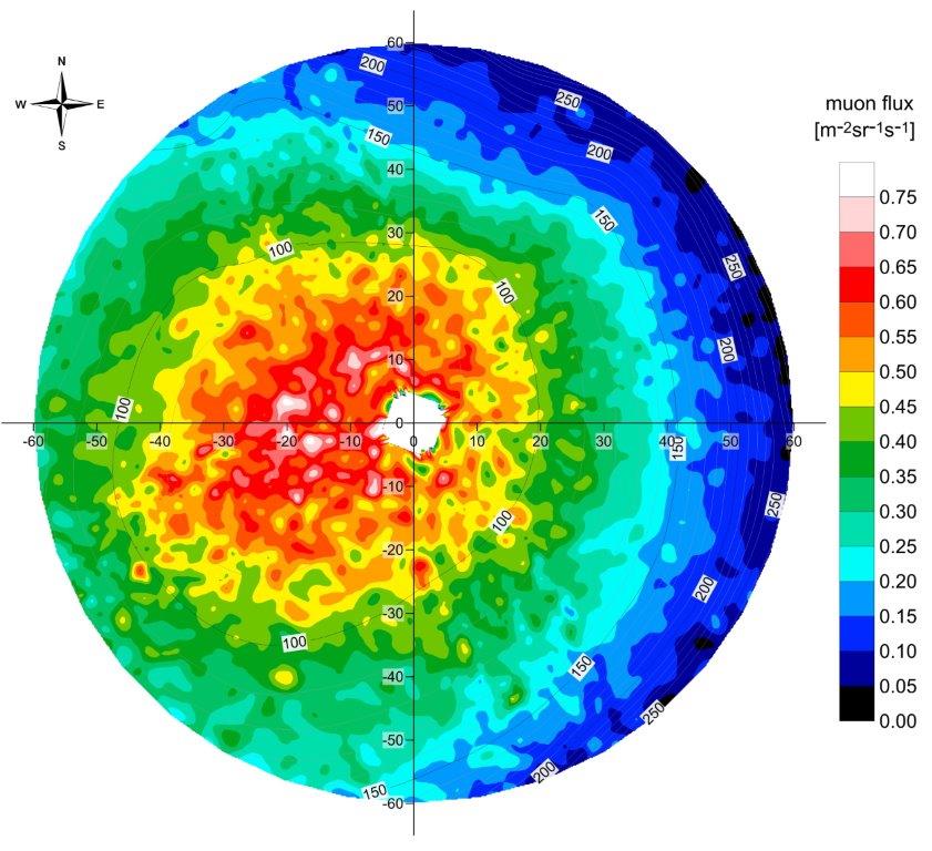
Figure 33. The cosmic muon flux map measured in MGGL is plotted as a function of azimuth and zenith angles from the detector position. Color-scale contours show the muon flux, dark contour lines show the detector-to-surface distance in meters. White areas show the out-of-acceptance directions. Left and right panels present the data respectively from the Run-0 and Run-1 measurements.

Merging all the data of Run-0 and Run-1 the muon flux distribution can be obtained, which is plotted in Fig. 34 up to zenith angle 60^∘. Correlation between muon flux map and the detector-to-distance contour lines is excellent. We found fluctuation is in the order of $\pm 0.05$ m^-2sr^-1s^-1 as it was obtained in Run-0 as well. One can observe that the surface distance and the muon flux reasonably match each other in Fig 34. Combining this with the acceptance plotted on the surface map plot on Fig. 32 the maximal flux matches the shortest distance-to-surface directions on the hill’s West slopes, while to the East, the muon flux drops at the large zenith angles with the longest traveling lengths.

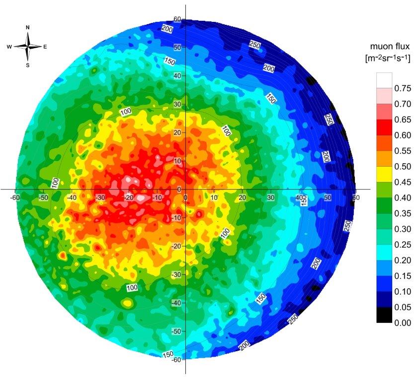
Figure 34. The cosmic muon flux map of Run-0 and Run-1 measured in MGGL plotted as a function of azimuth and zenith angles from the detector position. Color-scale contours show the muon flux, dark contour lines show the detector-to-surface distance in meters.

The collected $\sim 340,000$ tracks of the muon flux measurement provided high-enough statistics to estimate the rock thickness, based on the muon absorption model [55]. This model has been used successfully in other, similar measurements up to few 100 meters depth. In Fig. 35 the angular distribution of the rock density is presented. The average of the rock density is $2.6\pm 0.1$ kg dm^-3, which is the density of the andesite-based host rock. The data do not show any large-scale density inhomogeneities or cavities above the MGGL. However, minor, $\sim 0.2$ kg dm^-3, positive density deviation ridge is observed along the $40^{\circ}-50^{\circ}$ zenith angle from the southwest to northwest. This may correspond to several percent metallic ore in the unexplored part of the Gyöngyösoroszi mine. A negative $\sim 0.5$ kg dm^-3 density anomaly valley was also observed at the lowest $50^{\circ}-60^{\circ}$ zenith angle from the south to north. This is the direction of the known tunnels and caverns of the mine, although here the uncertainty of the measurement is also significant at large zenith angles.

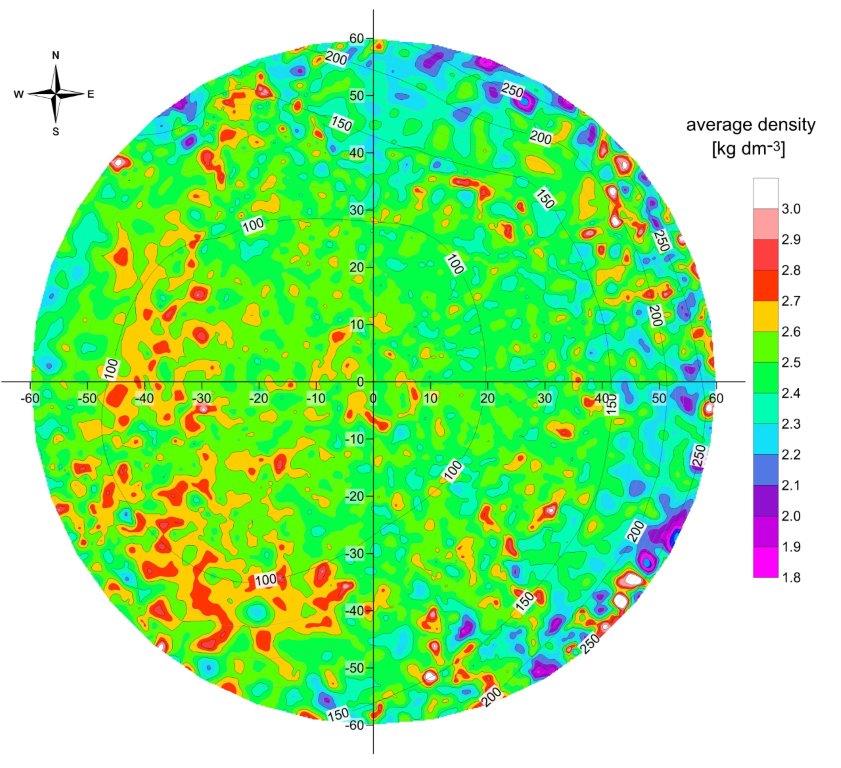
Figure 35. The angular distribution of the density based on Run-0 and Run-1 measured from the MGGL is plotted as a function of azimuth and zenith angles from the detector position. Color-scale contours show the rock densities, dark contour lines show the detector-to-surface distance in meters.

7.3. Conclusions

Based on the muon-flux measurements, the improved detector-to-surface date, and the muon absorption model, we can state, that the rock density map correlates well with the unexplored and mined areas above the MGGL. This unique measurement support to place the Einstein Telescope at Gyöngyösoroszi mine, since the lack of large-scale density inhomogenities would reduce the higher-order tensor-like gravitational corrections during the measurements.

8. Summary

The Mátra Gravitational and Geophysical Laboratory was established to investigate on a long term basis the conditions and requirements of next generation gravitational wave detectors in case of underground construction and operation. In more general, the aim was to measure various geological and rheological properties of the base rock in addition to test experimentally novel theoretical approaches on the noise penetration and suppression. Also the Mátra mountain range is studied as a possible site of the planned Einstein Telescope.

Our first investigations were published in Ref. [10] including the technical details of the measurements. In this paper we summarize the first two years of measurements of the laboratory by different methods: geophysical environment, electromagnetic attenuation, infrasound noise, cosmic muon tomography of the sorrounding rock mass, and long term seismic noise. The timeline of the data taking periods of the various measurements are shown in Fig. 36. Our topical results are:

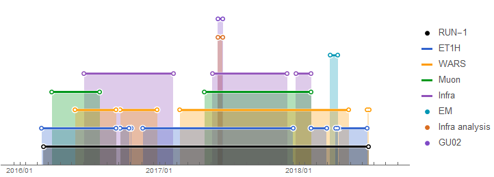
Figure 36. The data taking periods of the various measurements in MGGL during RUN-1.

Geophysical environment:

A short survey of the geological and seismological conditions in the Mátra mountains reveals a homogeneous composition of hard andesite rock with low seismic activity. We performed rock mechanic experiments and shown, that a typical grey andesite from the vicinity of the laboratory is not ideal elastic. We characterised and modeled the deviation from ideal elasticity and determined the corresponding rheological parameters (see Tables 3 and 4). The independent measurements of dynamic elastic moduli verify our novel rheological model, which properties are important when calculating the Newtonian noise from rock deformations.

Electromagnetic attenuation:

With EM noise measurements we estimated the electromagnetic attenuation by the andesite rock mass in the lower ELF range, especially at the frequency of the first Schumann resonance component. Comparing the data of the external surface reference station, we obtained the skin depth $3520$ m. For the bulk resistivity at the Schumann resonance frequency $387\Omega$m was obtained. This value – supporting the validity of this measurement – fits well to the literature value of vulcanic, andesite rocks ($170$-$45000$ $\Omega$m).

Infrasound noise:

Using the custom-made infrasound detector designed by the MTA Atomki, we measured the pressure amplitude spectral distribution in the MGGL (see Fig. 30). This is relatively noisy in the frequency range $1-7$ Hz. The recorded infrasound noise was found to be in accordance with the seismic noise at 3-4 Hz in the Laboratory.

Cosmic muon tomography:

During the 404 days long measurement with the Muontomograph merging Run-0 and Run-1 data, led us to map the rock density and its inhomogeneities above MGGL at large scale (see Fig. 35).We verified this novel measurement technique by obtaining the typical andesite rock density ($2.6\pm 0.1$ kg dm^-3). According to this investigations, we have found, there were no large scale density inhomogeneities ($\leq 0.2$ kg dm^-3) measured in the rock mass.

Seismic noise:

The long term seismic noise was registered by two seismometers inside the MGGL at depth $-88$ m almost for the whole two-years period. In parallel, as a cross check, a third seismometer measured the seismic noise for two-weeks duration. This data record were farther from the MGGL in the mine in $-404$ m depth. Seismic noise measurement were found to be consistent.

In the MGGL we had the opportunity to combine data taken at the same position, and in addition to this we could test the insights gained from noise analysis. According to our experience the proper evaluation of long term data requires some refinements of the methods applied in the ET Design Report [9]. Our suggestions has been published in Ref. [28] and in the recent study we evaluated the data accordingly. Therefore we calculated and show also the median of the spectra and the integrated noise measures $rms_{2-10\textrm{Hz}}$ and $rms_{1-10\textrm{Hz}}$ from the median, here. The analysis of the data from the Guralp ET1H and GU02 stations is based on these characteristics and the evaluation of the data from the WARS station also considered the problems of the more traditional methods.

We found, that the long term data does not show yearly changes in the median, but the intensity of the noisy periods reflects the changes in the activity inside the mine (see Fig. 10 and Tab. 7). The seasonal changes show minimal noise level in the late spring early summer period (see Fig. 11). The comparison of the noise level at the shallower and the deeper locations revealed that the two-weeks measurement is unexpectedly representative for the whole Run-0 and Run-1 period (see Fig. 13). We compared also working and night periods in MGGL in order to estimate an achievable minimum noise level (see Fig. 9). Considering our whole analysis the median spectrum of the night noise at -404m in the mine in Fig. 37 is convincingly representative in this respect. Here the percentiles are calculated from the spectra of the 50s long periods of data. One can see that in 90% of these periods the noise level is below the Black Forest line.

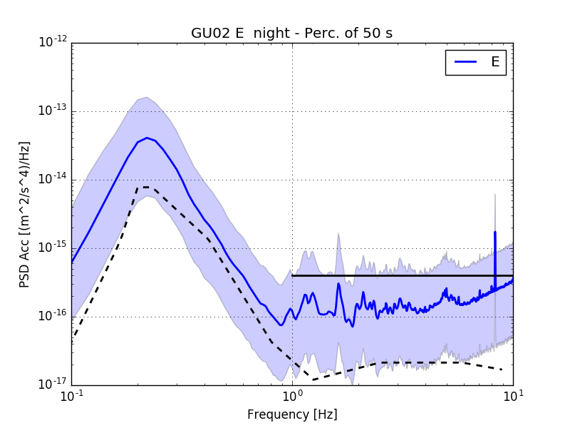
Figure 37. Acceleration ASD values of the representative two-week period of GU02 seismometer (-404 m), from the 50 s long night percentiles in one of the horizontal directions. The median is solid blue and the borderlines of the blue area are the 10^th and the 90^th percentiles. The dashed line is the NLNM curve of Peterson, the Black Forest line is solid black.

In general the noise levels our long term measurements in the shallower MGGL and also the two-week data from the deeper location are remarkably similar to the noise levels of the previous study [9, 25, 26], the mode $rms_{2Hz}$ are almost the same. As we have already mentioned, the median rms values are preferable, because they are more stable, less sensitive to the uncertainties is the data and in the evaluation. The ET1H and WARS median $rms_{2Hz}$ are close to each other. However, from the point of view of operational requirements, a higher percentile limit is a better estimation of the sensitivity of the detector for continuous operation. Therefore, the 90^th percentile rms values, given in Tab. 13, estimate the noise level for a continuous operation of the Einstein Telescope.

90th	GU02	ET1H 2ws	ET1H 2ys
$rms_{2Hz}[nm]$	0.171	0.257	0.261
$rms_{2-10Hz}[nm]$	0.167	0.243	0.238
$rms_{1-10Hz}[nm]$	0.401	0.600	0.583

Table 13. The $rms$ values of the 90^th percentile in the E direction with different frequency ranges for the MGGL seismometer ET1H and for the deeper location GU02, too. The first two columns are calculated from the $90\,th$ percentile of the $300\,s$ data of the two-week interval, the last one from the average of daily $90\,th$ percentiles.

According to the recent study a reliable and comparable characterisation of long term seismic noise data requires the evaluation of various noise measures with a uniform methodology. The separation of reducible and irreducible cultural noise, the seasonal changes and the attenuation by depth are important aspects for site description. Also it is very important to publish the raw seismological data for open evaluation and comparison. For the ET1H station of MGGL and for the GU02 station these are available at [56].

9. Conclusions

During the Run-0 and Run-1 periods of the MGGL in 2016-2018 we performed long-term monitoring the Mátra mountain range as a possible underground site of the planned Einstein Telescope. We used various standard methods in parallel to novel approaches of investigating the geophysical environment, electromagnetic attenuation, infrasound noise, cosmic muon tomography of the surrounding rock mass, and long term seismic noise. The collected data could enable us to cross check and and compare standard measurements and techniques applied in earlier investigations with the new ones. Alongside this, the geological and rheological properties of the base rock were summarized in this paper. In addition to the analysis of the noise background relevant for a next generation, underground-based gravitational wave detector, especially in the low frequency regime, at 1-10 Hz. We strongly believe that applying our results for the site selection will significantly improve the signal to nose ratio of the multi-messenger astrophysics era. Our conclusion was that for the background noise analysis, it is necessary to perform long term data taking and apply the state-of-the-art techniques presented here.

10. Acknowledgement

The contribution and support of Nitrokemia Zrt. in particular Á. Váradi and V. Rofrits is acknowledged. We also thank the construction work of Geofaber Zrt.

This research was supported by the MTA EUHUNKP grant. Authors PV and RK thank the Hungarian National Research, Development and Innovation Office NKFIH grants K124366, K104260, K116197, K120660, NK106119, and K116375 for funding. TB, MC, MS, DR and TS were supported by the NCN Grant UMO-2013/01/ASPERA/ST9/00001. The muon flux measurements have been supported by the Momentum ("Lendület") grant of the Hungarian Academy of Sciences under contract LP2013-60. The support of the PHAROS (CA16214) and G2net (CA17137) COST Actions is also acknowledged. We acknowledge the support of the grant TEAM/2016-3/19 from the Foundation for Polish Science. The support of the European Regional Development Fund and Hungary in the frame of the project GINOP-2.2.1-15-2016-00012 is acknowledged, too. We thank the Wigner GPU Laboratory for their help, too.

References

- [1] BP Abbott, R Abbott, TD Abbott, MR Abernathy, F Acernese, K Ackley, C Adams, T Adams, P Addesso, RX Adhikari, et al. Observation of gravitational waves from a binary black hole merger. Physical Review Letters, 116(6):061102, 2016.
- [2] BP Abbott, R Abbott, TD Abbott, MR Abernathy, F Acernese, K Ackley, C Adams, T Adams, P Addesso, RX Adhikari, et al. Gw151226: Observation of gravitational waves from a 22-solar-mass binary black hole coalescence. Physical Review Letters, 116(24):241103, 2016.
- [3] LIGO Scientific and Virgo Collaboration GW170104: Observation of a 50-Solar-Mass Binary Black Hole Coalescence at Redshift 0.2. Physical Review Letters, 118:221101, 2017.
- [4] LIGO Scientific and Virgo Collaboration GW170608: Observation of a 19 Solar-mass Binary Black Hole Coalescence ApJ Letters, 851:L35, 2017.
- [5] LIGO Scientific and Virgo Collaboration GW170814: A Three-Detector Observation of Gravitational Waves from a Binary Black Hole Coalescence Physical Review Letters, 119:141101, 2017.
- [6] LIGO Scientific and Virgo Collaboration GW170817: Observation of Gravitational Waves from a Binary Neutron Star Inspiral Physical Review Letters, 119:161101, 2017.
- [7] Technical report. http://gwcenter.icrr.u-tokyo.ac.jp/en/.
- [8] Technical report. http://www.et-gw.eu/index.php/letter-of-intent.
- [9] ET Science Team. Einstein gravitational wave Telescope, Conceptual Design Study. Technical Report ET-0106C-10, June 2011. http://www.et-gw.eu/etdsdocument.
- [10] G.G. Barnaföldi, T. Bulik, M. Cieslar, E. Dávid, M. Dobróka, E. Fenyvesi, Z. Gráczer, G. Hamar, G. Huba, Á. Kis, R. Kovács, I. Lemperger, P. Lévai, J. Molnár, D. Nagy, A. Novák, L. Oláh, P. Pázmándi, D. Piri, D. Rosinska, L. Somlai, T. Starecki, M. Suchenek, G. Surányi, S. Szalai, D. Varga, M. Vasúth, P. Ván, B. Vásárhelyi, V. Wesztergom, and Z. Wéber. First report of long term measurements of the MGGL laboratory in the Mátra mountain range. Classical and Quantum Gravity, 34:114001(22), 2017. arXiv: 1610.07630.
- [11] I. Kovács and C. Szabó. Middle miocene volcanism in the vicinity of the middle Hungarian zone: evidence for an inherited enriched mantle source. Journal of Geodynamics, 45(1):1–17, 2008.
- [12] MTA CSFK GGI, Earthquake Catalogue, Geodetic and Geophysical Institute, Research Centre for Astronomy and Earth Sciences, Hungarian Academy of Sciences, Sopron, Hungary, 2018.
- [13] Gráczer et al. Hungarian national seismological bulletins (2011-2017). Technical report, MTA CSFK GGI Kövesligethy Radó Seismological Observatory, Budapest, 2012-2018.
- [14] Z. Gráczer, G. Szanyi, I. Bondár, C. Czanik, T. Czifra, E. Győri, Gy. Hetényi, I. Kovács, I. Molinari, B. Süle, E. Szűcs, V. Wesztergom, and Z. Wéber. AlpArray in Hungary: temporary and permanent seismological networks in the transition zone between the Eastern Alps and the Pannonian basin. Acta Geodaetica et Geophysica, 2018. under publication.
- [15] D. Giardini, J. Woessner, and Danciu. Mapping Europe’s seismic hazard. Transactions American Geophysical Union, 95(29):261–262, 2014.
- [16] D. Giardini, L. Woessner, J. amd Danciu, H. Crowley, F. Cotton, G. Grünthal, and R. Basili. Seismic hazard harmonization in Europe (share): Online data resource. Technical report, 2013.
- [17] RD Lama and VS Vutukuri. Handbook on mechanical properties of rocks Testing techniques and results II., volume 2. 1978.
- [18] AI Savich. Generalized relations between static and dynamic indices of rock deformability. Hydrotechnical Construction, 18(8):394–400, 1984.
- [19] WL van Heerden. General relations between static and dynamic moduli of rocks. International Journal of Rock Mechanics and Mining Sciences & Geomechanics Abstracts, 24(6):381–385, 1987.
- [20] A Mockovčiaková and B Pandula. Study of the relation between the static and dynamic moduli of rocks. Metalurgija, 42(1):37–39, 2003.
- [21] H Gercek. Poisson’s ratio values for rocks. International Journal of Rock Mechanics and Mining Sciences, 44(1):1–13, 2007.
- [22] Ali Reza Najibi, Mohammad Ghafoori, Gholam Reza Lashkaripour, and Mohammad Reza Asef. Empirical relations between strength and static and dynamic elastic properties of Asmari and Sarvak limestones, two main oil reservoirs in Iran. Journal of Petroleum Science and Engineering, 126:78–82, 2015.
- [23] Cs. Asszonyi, T. Fülöp, and P. Ván. Distinguished rheological models for solids in the framework of a thermodynamical internal variable theory. Continuum Mechanics and Thermodynamics, 27:971–986, 2015. arXiv:1407.0882.
- [24] Ömer Aydan, Takashi Ito, Ugur Özbay, M. Kwasniewski, K. Shariar, T. Okuno, A. Özgenoğlu, D.F. Malan and t. Okada. ISRM suggested methods for determining the creep characteristics of rock Rock mechanics and rock engineering, 47/1:275–290, 2014.
- [25] M. G. Beker. Low-frequency sensitivity of next generation gravitational wave detectors. PhD thesis, Vrije Universiteit Amsterdam, Amsterdam, June 2013.
- [26] M. G. Beker, J. F. J. van den Brand, and D. S. Rabeling. Subterranean ground motion studies for the Einstein Telescope. Classical and Quantum Gravity, 32(2):025002, 2015.
- [27] Technical report. See the manual of the instrument: http://www.guralp.com/documents/DAS-030-0120.pdf.
- [28] L. Somlai, Y. Gráczer, M. Vasúth, Y. Wéber, and P. Ván. Silence measurements and measures for ET: characterisation of long term seismic noise in the Mátra Mountains. 2018. arXiv:1804.07200.
- [29] J. Peterson. Observations and modeling of seismic background noise. Open-File Report, 1993, USGS, 93-322.
- [30] Gerhard Heinzel, Albrecht Rüdiger, and Roland Schilling. Spectrum and spectral density estimation by the discrete Fourier transform (DFT), including a comprehensive list of window functions and some new at-top windows. Report 2002.
- [31] P. Welch. The use of fast Fourier transform for the estimation of power spectra: A method based on time averaging over short, modified periodograms. IEEE Transactions on Audio and Electroacoustics, 15(2):70–73, June 1967.
- [32] Ralph Beebe Blackman and John W Tukey. The measurement of power spectra. Dover, 1958.
- [33] Ernest R Kanasewich. Time sequence analysis in geophysics. University of Alberta, 1981.
- [34] E. Thrane, N. Christensen, and R. M. S. Schofield. Correlated magnetic noise in global networks of gravitational-wave detectors: Observations and implications. Physical Review D, 87(12), June 2013.
- [35] W.O. Schumann. On the free oscillation of a conducting sphere, which is surrounded by an air layer and an ionospheric shell. Z. Naturforschung, 7a:149–154, 1952.
- [36] A. Kulak, J. Kubisz, S. Klucjasz, A. Michalec, J. Mlynarczyk, Z. Nieckarz, M. Ostrowski, and S. Zieba. Extremely low frequency electromagnetic field measurements at the Hylaty station and methodology of signal analysis. Radio Science, 49:361–370, 2014. See also http://www.oa.uj.edu.pl/elf/index/projects1.htm.
- [37] Vincent Mazet, Cédric Carteret, David Brie, Jérôme Idier, and Bernard Humbert. Background removal from spectra by designing and minimising a non-quadratic cost function. Chemometrics and Intelligent Laboratory Systems, 76(2):121–133, 2005.
- [38] K. Vozoff. The Magnetotelluric Method. 1991.
- [39] Louis B. Slichter and M. Telkes. Electrical Properties of Rocks and Minerals. 1942.
- [40] Peter R. Saulson. Terrestrial gravitational noise on a gravitational wave antenna. Phys. Rev. D, 30:732–736, 1984.
- [41] J. R. Bowman, G. E. Baker, and M. Bahavar. Ambient infrasound noise. Geophysical Research Letters, 32(9).
- [42] The new generation of microbarometer with remote calibration capability.
- [43] I. Bodnár and Cs. Czanik. Hungarian national infrasound network.
- [44] C. Leys, C. Ley, O. Klein, P. Bernard and L. Licata. Detecting outliers: Do not use standard deviation around the mean, use absolute deviation around the median. Journal of Experimental Social Psychology 49(4):764 - 766, 2013.
- [45] P. Welch. The use of fast fourier transform for the estimation of power spectra: A method based on time averaging over short, modified periodograms. IEEE Transactions on Audio and Electroacoustics, 15(2):70–73, June 1967.
- [46] G. G. Barnaföldi et al., First report of long term measurements of the MGGL laboratory in the Mátra mountain range Class. Quant. Grav. 34, no. 11, 114001 (2017)
- [47] G. G. Barnaföldi et al. Portable cosmic muon telescope for environmental applications Nucl. Instrum. Meth. A689:60-69 (2012)
- [48] L. Oláh et al. CCC-based muon telescope for examination of natural caves Geosci. Instrum. Method. Data Syst. 1:229-234 (2012)
- [49] L. Oláh et al. Cosmic Muon Detection for Geophysical Applications Adv. in High Energy Physics V2013, 560192(7) (2013)
- [50] L. Oláh et al. Close Cathode Chamber technology for cosmic particle tracking Journal of Physics: Conference Series 632:012020 (2015)
- [51] L. Oláh et al. Cosmic Background Measurements at a Proposed Underground Laboratory by the REGARD Muontomograph Journal of Physics: Conference Series 665:012032 (2016)
- [52] L. Oláh et al. High-definition and low-noise muography of the Sakurajima volcano with gaseous tracking detectors Scientific Reports 8, 3207 (2018)
- [53] D. Varga et al. Asymmetric Multi-Wire Proportional Chamber with reduced requirements to mechanical precision Nucl. Instrum. Meth. A648:163-167 (2011)
- [54] D. Varga et al. Close cathode chamber: Low material budget MWPC Nucl. Instrum. Meth. A698:11-18 (2013)
- [55] A. Tang et al. Muon simulations for Super-Kamiokande, KamLAND and CHOOZ Phys. Rev. D 74, 053007 (2006)
- [56] The seismological data of RUN-1 are here: https://mydrive.kfki.hu/d/453f675ba7db47adb2b3/.