The Properties of Parsec-Scale Blazar Jets

Abstract

I show that by assuming a standard Blandford-Königl jet, it is possible to determine the bulk Lorentz factor and angle to the line of sight of self-similar parsec-scale blazar jets by using five measured quantities: redshift, core radio flux, extended radio flux, the magnitude of the core shift between two frequencies, and apparent jet opening angle. From the bulk Lorentz factor and angle computed with this method, one can compute other jet properties such as the Doppler factor, magnetic field strength, and intrinsic jet opening angle. I use data taken from the literature and marginalize over nuisance parameters associated with the electron distribution and equipartition to compute these quantities, although the errors are large. Results are generally consistent with constraints from other methods. Primary sources of uncertainty are the errors on the core shift measurements and the uncertainty in the electron spectral index.

1. Introduction

Blazars are active galactic nuclei with relativistic jets oriented close to our line of sight. They are associated with compact jet components on the milliarcsecond scale that can be resolved with radio very long baseline interferometry (VLBI). VLBI images of these objects reveal a stationary core from which knots emerge. Often the apparent speeds of these knots projected on the sky $\beta_{\rm app}c>1$, i.e., they appear to be moving faster than the speed of light $c$. This is a well-known optical illusion caused by motion with intrinsic speed $\beta c$ close to $c$ and angle to the line of sight $\theta\ll 1$ (Rees, 1966).

One of the defining features of blazars is their bright, stationary cores seen in VLBI images. This core is generally thought to be described by the Blandford-Königl (BK) model (Blandford & Königl, 1979; Königl, 1981). In this model, the core emission is the superposition of self-absorbed components in a steady, continuous parsec-scale jet. This model is likely a useful approximation to reality: a model where a number of colliding shells in the jet accelerate electrons, which cool through radiative and adiabatic losses can reproduce many of the features of the BK model (Jamil et al., 2010).

The BK model makes two key predictions. The first is flat radio spectra ($\alpha\approx 0$, where the radio flux density $F_{\nu}\propto\nu^{-\alpha}$ and $\nu$ is the observed frequency). The observation of flat spectra in blazar cores was the primary empirical motivation for the model. The second is a frequency-dependent core position; that is, the core’s position on the sky will “shift” between two different positions when viewed at different frequencies. This effect has also been observed in a number of blazar radio cores (e.g., Lobanov, 1998; Kovalev et al., 2008; O’Sullivan & Gabuzda, 2009; Sokolovsky et al., 2011; Pushkarev et al., 2012). When observed at multiple frequencies, the magnitude of the core shift is observed to be $\propto\nu^{-1}$, in agreement with the BK model prediction (O’Sullivan & Gabuzda, 2009; Sokolovsky et al., 2011).

The magnitudes of the core shifts have been used to infer the magnetic field of the jet (e.g., Pushkarev et al., 2012; Zdziarski et al., 2015). This usually requires making some assumption about the jet speed (bulk Lorentz factor, $\Gamma$) or orientation (angle to the line of sight, $\theta$). Here I show that it is in fact not necessary to make assumptions about the speed and orientation of blazar jets. Assuming the BK model is a reasonable description of these jets, one can determine $\Gamma$, $\theta$, and other jet parameters such as the magnetic field, from five observables: the redshift $z$, the core flux density $F_{\nu}$, the core shift $\Delta\phi$, the apparent opening angle for the jet $\alpha_{\rm app}$, and the extended radio flux, which is used as a proxy for jet power (e.g., Bîrzan et al., 2004, 2008; Cavagnolo et al., 2010).

In Section 2 I describe the BK jet model and show how it can be used to determine jet parameters from the observables. In Section 3 this model is applied to a sample of blazar radio jets with appropriate observations from the literature. The measured properties of their jets, including $\Gamma$ and $\theta$ are presented. In Section 4 I compare my results with previous estimates of these parameters, and explore some of the implications of the results. Finally, I conclude with a discussion in Section 5.

2. Continuous Jet Model

2.1. Synchrotron Self-Absorption

In the $\delta$-function approximation, synchrotron self-absorption (SSA) opacity at a dimensionless energy $\epsilon=h\nu/(m_{e}c^{2})\approx\nu/(1.23\times 10^{20}\ \mathrm{Hz})$ is

$$\kappa(\epsilon)=\frac{-\pi}{36}\frac{\lambda_{C}r_{e}}{\epsilon}\left\{\gamma\frac{\partial}{\partial\gamma}\left[\frac{n_{e}(\gamma)}{\gamma^{2}}\right]\right\}\Biggr{|}_{\gamma=\sqrt{\epsilon/(2\epsilon_{B})}}\$$ (1)

(Dermer & Menon, 2009) where $r_{e}\approx 2.8\times 10^{-13}\ \mathrm{cm}$ is the classic electron radius, $\lambda_{C}\approx 2.4\times 10^{-10}\ \mathrm{cm}$, $\epsilon_{B}=B/B_{c}$, $B$ is the magnetic field, and $B_{c}=4.414\times 10^{13}\ \mathrm{G}$. Let the electron density distribution be a power-law, $n_{e}(\gamma)=n_{0}\gamma^{-p}H(\gamma;\gamma_{1},\gamma_{2})$ where

$$H(x;a,b)=\left\{\begin{array}[]{ll}1&a<x<b\\ 0&\mathrm{otherwise}\end{array}\right.\ .$$ (2)

Then

$$\kappa(\epsilon) =C(p)\lambda_{c}r_{e}\epsilon^{-(p+4)/2}\epsilon_{B}^{(p+2)/2}n_{0}\$$ (3)

$$\times H[\sqrt{\epsilon/(2\epsilon_{B})};\gamma_{1},\gamma_{2}]$$

where

$$C(p)=\frac{\pi}{18}(p+2)(2)^{p/2}\ .$$ (4)

This can be compared with more precise expressions by, e.g., Gould (1979) and Zdziarski et al. (2012a).

2.2. Continuous Jet

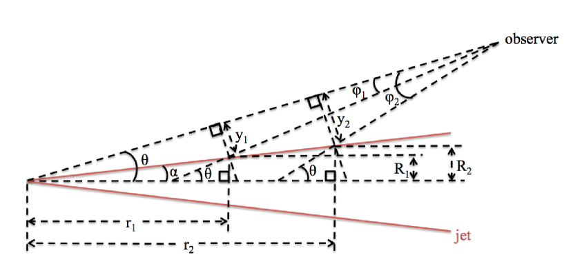
Figure 1.— Cross-section illustration of conical jet geometry.

Consider a conical continuous relativistic jet with half-opening angle $\alpha\ll 1$; see Figure 1 for an illustration of the geometry. The source has cosmological redshift $z$ giving it a luminosity distance

$$d_{L}=(1+z)\frac{c}{H_{0}}\int_{0}^{z}\frac{dz^{\prime}}{\sqrt{\Omega_{m}(1+z^{\prime})^{3}+\Omega_{\Lambda}}}\ .$$ (5)

I use $H_{0}=70\ \mathrm{km}\ \mathrm{s}^{-1}\ \mathrm{Mpc}^{-1}$, $\Omega_{m}=0.3$, and $\Omega_{\Lambda}=0.7$. If a core shift is observed it implies $\alpha<\theta$. Since I am interested in the case where a core shift is indeed observed, I assume this is the case. The distance from the base of the jet is $r$ and the half width of the jet at $r$ is $R$, so that $R/r=\tan\alpha\approx\alpha$. The jet moves with speed $\beta c$ giving it a bulk Lorentz factor $\Gamma=(1-\beta)^{-1/2}$. The electron density and magnetic field in the jet are assumed to decrease with $r$, so that

$$n_{0}=n_{00}\ \tilde{r}^{-a}\ ,$$ (6)

$$\epsilon_{B}=\epsilon_{B0}\ \tilde{r}^{-b}$$ (7)

where $\tilde{r}=r/r_{0}$, $r_{0}$ is some reference distance along the jet, $n_{00}=n_{0}(r_{0})$, and $\epsilon_{B0}=\epsilon_{B}(r_{0})$. The half-jet width at $r_{0}$ is $R_{0}=\alpha r_{0}$.

An observer sees the jet at an angle $\theta$ to the center of the jet axis, so that the Doppler factor $\delta_{\rm D}=[\Gamma(1-\beta\cos\theta)]^{-1}$ and the apparent half-opening angle

$$\alpha_{\rm app}=\alpha/\sin\theta\ .$$ (8)

Hereafter, in the frame co-moving with the jet, quantities are primed, such as the co-moving distance from the jet base, $r^{\prime}$. Quantities in the rest frame of the galaxy are unprimed, except for energies, where unprimed quantities are in the observer frame, so that $\epsilon=\epsilon^{\prime}\delta_{\rm D}/(1+z)$. The difference between the observer frame and galaxy frame is a factor $1+z$.

2.3. Synchrotron Self-Absorption in Continuous Jet

The absorption optical depth

$$\tau(\epsilon^{\prime})=\int d\ell^{\prime}\ \kappa^{\prime}(\epsilon^{\prime})$$ (9)

where $\ell^{\prime}$ is the distance a photon travels in the jet to the observer, in the co-moving frame. The angle to the line of sight in the comoving frame is transformed as $\sin\theta^{\prime}=\delta_{\rm D}\sin\theta$ (e.g., Rybicki & Lightman, 1979; Zdziarski et al., 2012a). In the frame of the galaxy $\ell=R/\sin\theta=r\alpha_{\rm app}$. Using Equation (3) for $\kappa(\epsilon^{\prime})$, the SSA opacity, and with a change of variables from $\ell^{\prime}$ to $r$, Equation (9) can be integrated to give

$$\tau(\epsilon) =C(p)\alpha_{\rm app}k_{1}^{-1}\lambda_{C}r_{e}(1+z)^{-(p+4)/2}\delta_{\rm D}^{(p+2)/2}$$ (10)

$$\times\epsilon_{B0}^{(p+2)/2}\epsilon^{-(p+4)/2}\tilde{r}^{-k_{1}}n_{00}r_{0}$$

where $k_{1}=b(p+2)/2+a-1$. Equation (10) can be compared to Equation (1) of Lobanov (1998) and Equation (26) of Blandford & Königl (1979). By setting $\tau(\epsilon)=1$ in Equation (10) one can solve for the energy where the jet becomes optically thin to synchrotron self-absorption,

$$\epsilon_{\rm SSA}=\epsilon_{\rm SSA,0}\ \tilde{r}^{-k_{2}}$$ (11)

where

$$\epsilon_{\rm SSA,0}= \left[\frac{C(p)\lambda_{C}r_{e}n_{00}R_{0}}{\sin\theta k_{1}}\right]^{2/(p+4)}$$ (12)

$$\times(\delta_{\rm D}\epsilon_{B0})^{(p+2)/(p+4)}\frac{1}{1+z}\ ,$$

$$k_{2}=\frac{2k_{1}}{p+4}=\frac{2a+b(p+2)-2}{p+4}\ ,$$ (13)

and $R_{0}=\alpha r_{0}$.

2.4. Core Shift

In the context of the BK model, the core is the surface where $\tau=1$. The observed angular distance of a core from the base of the jet observed at a given observed dimensionless energy $\epsilon_{\rm SSA}$ is

$$\phi=\frac{r\sin\theta}{d_{A}}=\frac{R_{0}}{\alpha_{\rm app}d_{A}}\left(\frac{\epsilon_{SSA,0}}{\epsilon_{SSA}}\right)^{1/k_{2}}$$ (14)

where $d_{A}=d_{L}/(1+z)^{2}$ is the angular diameter distance. The core shift between two dimensionless energies $\epsilon_{\rm SSA,1}$ and $\epsilon_{\rm SSA,2}$ where $\epsilon_{\rm SSA,2}<\epsilon_{\rm SSA,1}$ is then

$$\Delta\phi =\phi_{2}-\phi_{1}=\frac{R_{0}(1+z)^{2}}{\alpha_{\rm app}d_{L}}\epsilon_{SSA,0}^{1/k_{2}}\left(\frac{1}{\epsilon_{SSA,2}^{1/k_{2}}}-\frac{1}{\epsilon_{SSA,1}^{1/k_{2}}}\right)$$

$$=\frac{R_{0}(1+z)^{2}}{\alpha_{\rm app}d_{L}}\left(\frac{\epsilon_{\rm SSA,0}}{\epsilon_{\rm eff}}\right)^{1/k_{2}}$$ (15)

where

$$\epsilon_{\rm eff}=\frac{\epsilon_{\rm SSA,2}\epsilon_{\rm SSA,1}}{\left(\epsilon_{\rm SSA,1}^{1/k_{2}}-\epsilon_{\rm SSA,2}^{1/k_{2}}\right)^{k_{2}}}\ .$$ (16)

The geometry of this core shift is illustrated in Figure 1. For the “standard” continuous BK jet, $a=2$ and $b=1$ (Blandford & Königl, 1979; Königl, 1981) gives $k_{2}=1$, in agreement with core shift observations (O’Sullivan & Gabuzda, 2009; Sokolovsky et al., 2011).

2.5. Flux of Continuous Jet

For a continuous relativistic jet with stationary pattern, the observed $\nu F_{\nu}$ flux

$$f_{\epsilon}^{sy}=\frac{\delta_{\rm D}^{3}}{4\pi d_{L}^{2}\Gamma}\int dV^{\prime}\ \epsilon^{\prime}\ j^{\prime}(\epsilon^{\prime})\ ,$$ (17)

(Sikora et al., 1997; Zdziarski et al., 2012a, b) where $\epsilon^{\prime}j^{\prime}(\epsilon^{\prime})$ is the comoving frame emissivity (from synchrotron in this case), and the comoving volume $dV^{\prime}=\Gamma dV$. For a conical jet, $dV=\pi R^{2}dr$. It is well-known that for synchrotron emission, $F_{\nu}\propto\nu^{5/2}$ in the SSA optically thick ($\tau>1$) regime and $F_{\nu}\propto\nu^{-(p-1)/2}$ in the SSA optically thin ($\tau<1$) regime. To account for both these regimes, I approximate the emission from a jet volume element $dV^{\prime}$ as

$$\epsilon^{\prime}j^{\prime}(\epsilon^{\prime})\approx 2c\sigma_{\rm T}u_{B}/3$$

$$\times\left\{\begin{array}[]{ll}\gamma^{\prime 3}_{\rm SSA}n_{e}(\gamma^{\prime}_{\rm SSA})\left(\epsilon^{\prime}/\epsilon^{\prime}_{\rm SSA}\right)^{7/2}&\epsilon^{\prime}<\epsilon^{\prime}_{\rm SSA}\\ \gamma^{\prime 3}n_{e}(\gamma^{\prime})&\epsilon^{\prime}_{\rm SSA}<\epsilon^{\prime}\\ \end{array}\right.\ ,$$ (20)

where

$$\gamma^{\prime}=\sqrt{\frac{\epsilon^{\prime}}{\epsilon_{B}}}\ ,$$ (21)

$$\gamma^{\prime}_{\rm SSA}=\sqrt{\frac{\epsilon^{\prime}_{\rm SSA}}{\epsilon_{B}}}\ ,$$ (22)

$$u_{B}=\frac{B^{2}}{8\pi}=u_{\rm Bcr}\epsilon_{B}^{2}$$ (23)

is the Poynting flux energy density, and

$$u_{\rm Bcr}=\frac{B_{c}^{2}}{8\pi}\ .$$ (24)

Note that $B$ and $\epsilon_{B}$ are in the comoving frame, although I neglect the primes on them. Substituting Equations (2.5) into Equation (17),

$$f_{\epsilon}^{sy} =\frac{\delta_{\rm D}^{3}n_{0}c\sigma_{\rm T}u_{\rm Bcr}R^{2}}{6d_{L}^{2}}$$

$$\times\Biggr{\{}\int_{r_{\min}}^{r_{b}}dr\ \epsilon_{B}^{(1+p)/2}\epsilon_{\rm SSA}^{\prime(3-p)/2}\left(\frac{\epsilon^{\prime}}{\epsilon^{\prime}_{\rm SSA}}\right)^{7/2}$$

$$+\int_{r_{b}}^{r_{\max}}dr\ \epsilon_{B}^{(1+p)/2}\epsilon^{\prime(3-p)/2}\Biggr{\}}\ ,$$ (25)

where $r_{\min}$ is the distance from the base of the jet where emission begins, $r_{\max}$ is the distance from the base of the jet where emission ends, and $r_{b}=(\epsilon^{\prime}_{\rm SSA,0}/\epsilon^{\prime})^{1/k_{2}}$. Using Equation (11) and performing the integrals assuming $r_{\min}\ll r_{b}\ll r_{\max}$,

$$f_{\epsilon}^{sy} =\frac{\delta_{\rm D}^{3}c\sigma_{\rm T}u_{\rm Bcr}R_{0}^{2}r_{0}n_{00}\epsilon_{B0}^{(1+p)/2}}{3d_{L}^{2}}$$

$$\times\Biggr{\{}\frac{\epsilon^{\prime 7/2}\epsilon_{\rm SSA,0}^{\prime-(p+4)/2}}{6+k_{2}(p+4)-b(p+1)-2a}$$

$$\times\left(\frac{\epsilon^{\prime}_{SSA,0}}{\epsilon^{\prime}}\right)^{\frac{6+k_{2}(p+4)-b(p+1)-2a}{2}}$$

$$+\frac{\epsilon^{\prime(3-p)/2}}{b(p+1)+2a-6}\left(\frac{\epsilon^{\prime}_{\rm SSA,0}}{\epsilon^{\prime}}\right)^{\frac{6-b(p+1)-2a}{2}}\Biggr{\}}\ .$$ (26)

For the standard BK jet, $a=2$, $b=1$, and $k_{2}=1$,

$$\frac{f_{\epsilon}^{sy}}{\epsilon} =\delta_{\rm D}^{(3+p)/2}c\sigma_{\rm T}u_{\rm Bcr}R_{0}^{2}r_{0}n_{00}\epsilon_{B0}^{(1+p)/2}\epsilon_{SSA,0}^{(1-p)/2}$$

$$\times\left[\frac{(1+z)^{(3-p)/2}}{3d_{L}^{2}}\right]\left[\frac{p+4}{5(p-1)}\right]\ .$$ (27)

The flux density $F_{\nu}$ can be found directly from Equation (2.5), since

$$F_{\nu}=\frac{f_{\epsilon}^{sy}}{\epsilon}\frac{h}{m_{e}c^{2}}\ .$$ (28)

Thus, $F_{\nu}$ will be independent of $\nu$ (or $\epsilon$), i.e., “flat” in agreement with observations of the radio spectra of the cores of blazars. Equation (2.5) agrees with similar formulations by a number of other authors (e.g., Blandford & Königl, 1979; Königl, 1981; Falcke & Biermann, 1995; Zdziarski et al., 2012a). This calculation only accounts for a single jet traveling towards the observer, neglecting the counter-jet emission (cf. Zdziarski et al., 2012a).

2.6. Jet Power

The jet power from a single jet

$$P_{j} =\hat{\gamma}_{\rm ad}\pi R^{2}\Gamma^{2}\beta c$$

$$\times\left(g_{B}u_{B}+u_{e}+u_{p}+\frac{\Gamma-1}{\hat{\gamma}_{\rm ad}\Gamma}\rho c^{2}\right)$$ (29)

where $\hat{\gamma}_{\rm ad}$ is the adiabatic index, $g_{B}\sim 1$ is a factor taking into account the geometry of the magnetic field,

$$u_{e}=m_{e}c^{2}\int d\gamma\ \gamma\ n_{e}(\gamma)=m_{e}c^{2}n_{0}A(p,\gamma_{1},\gamma_{2})\$$ (30)

is the electron energy density,

$$A(p,\gamma_{1},\gamma_{2})=\left\{\begin{array}[]{ll}(p-2)^{-1}(\gamma_{1}^{2-p}-\gamma_{2}^{2-p})&p\neq 2\\ \ln(\gamma_{2}/\gamma_{1})&p=2\end{array}\right.\ ,$$ (31)

$u_{p}$ is the relativistic proton energy density, and $\rho$ is the mass density (see Bicknell, 1994; Zdziarski, 2014, for a description of this term). The adiabatic index in Equation (2.6) takes into account the contribution from both the pressure and energy density (e.g. Levinson, 2006; Zdziarski et al., 2012a; Zdziarski, 2014). I use $\hat{\gamma}_{\rm ad}=4/3$ for a relativistic plasma and $g_{B}=1.5$ for a toroidal magnetic field (e.g., Levinson, 2006; Zdziarski et al., 2015). I define $\xi_{e}\equiv u_{e}/u_{B}$, $\xi_{p}\equiv u_{p}/u_{B}$, and $\xi_{m}\equiv\rho c^{2}/(\hat{\gamma}_{\rm ad}u_{B})$, so that

$$P_{j} =\hat{\gamma}_{\rm ad}\pi R^{2}\Gamma^{2}\beta cu_{B}$$ (32)

$$\times\left(g_{B}+\xi_{e}+\xi_{p}+\frac{\Gamma-1}{\Gamma}\xi_{m}\right)\ .$$

The jet power $P_{j}$ can be estimated from the power needed to inflate a cavity in the hot X-ray emitting intracluster medium, and is correlated with the extended radio luminosity of a radio-loud AGN (e.g., Bîrzan et al., 2004, 2008; Cavagnolo et al., 2010). The relationship between the jet power $P_{j}$ and the 200-400 MHz extended luminosity $L_{\rm ext}$ is

$$\log_{10}\left[\frac{P_{j}}{\mathrm{erg}\ \mathrm{s}^{-1}}\right]=c_{1}\left\{\log_{10}\left[\frac{L_{\rm ext}}{\mathrm{erg}\ \mathrm{s}^{-1}}\right]-40\right\}+c_{2}\ ,$$ (33)

where $c_{1}=0.64\pm 0.09$ and $c_{2}=43.54\pm 0.12$ (Cavagnolo et al., 2010). I use this expression to estimate the jet power from $L_{\rm ext}$. I divide the power obtained from Equation (33) by 2 to account for only a single jet.

Using Equation (2.6), Equation (12) can be written

$$\epsilon_{SSA,0} =\left[\frac{C(p)\lambda_{C}r_{e}}{\sin\theta k_{1}m_{e}c^{2}A(p,\gamma_{1},\gamma_{2})\Gamma^{2}}\right]^{\frac{2}{p+4}}$$

$$\times\frac{1}{1+z}\left(\frac{\delta_{\rm D}}{\Gamma}\right)^{\frac{p+2}{p+4}}\left(\frac{P_{j}}{\hat{\gamma}_{\rm ad}\pi\beta c}\right)^{\frac{p+6}{2(p+4)}}$$

$$\times\frac{1}{R_{0}\chi_{1}}\left(\frac{1}{u_{\rm Bcr}}\right)^{\frac{p+2}{2(p+4)}}\ ,$$ (34)

where

$$\chi_{1} =\xi_{e}^{\frac{-2}{p+4}}\left(g_{B}+\xi_{e}+\xi_{p}+\xi_{m}\frac{\Gamma-1}{\Gamma}\right)^{\frac{p+6}{2(p+4)}}\ .$$ (35)

For the $a=2$, $b=1$ model,

$$P_{j} =\hat{\gamma}_{\rm ad}\pi R_{0}^{2}\Gamma^{2}\beta cu_{\rm Bcr}\epsilon_{B0}^{2}$$

$$\times\left(g_{B}+\xi_{e}+\xi_{p}\xi_{m}\frac{\Gamma-1}{\Gamma}\right)$$

$$=\hat{\gamma}_{\rm ad}\pi R_{0}^{2}\Gamma^{2}\beta cm_{e}c^{2}n_{00}A(p,\gamma_{1},\gamma_{2})$$

$$\times\left(1+\frac{g_{B}}{\xi_{e}}+\frac{\xi_{p}}{\xi_{e}}+\frac{\xi_{m}}{\xi_{e}}\frac{\Gamma-1}{\Gamma}\right)\ .$$ (36)

2.7. Determination of Jet Parameters

Combining Equations (2.4) and (2.6) for the the $a=2$, $b=1$ model, with some algebraic manipulation,

$$\Delta\phi =\frac{1+z}{\epsilon_{\rm eff}\alpha_{\rm app}d_{L}\chi_{1}}\left[\frac{C(p)\lambda_{C}r_{e}}{\sin\theta k_{1}m_{e}c^{2}A(p,\gamma_{1},\gamma_{2})\Gamma^{2}}\right]^{\frac{2}{p+4}}$$

$$\times\left[\frac{\delta_{\rm D}}{\Gamma}\right]^{\frac{p+2}{p+4}}\left[\frac{P_{j}}{\hat{\gamma}_{\rm ad}\pi\beta c}\right]^{\frac{p+6}{2(p+4)}}\left[\frac{1}{u_{\rm Bcr}}\right]^{\frac{p+2}{2(p+4)}}\ .$$ (37)

Similarly, combining Equations (2.5), (2.4), and (2.6), and more algebraic manipulation,

$$\frac{f_{\epsilon}^{sy}}{\epsilon} =\frac{c\sigma_{\rm T}}{3\chi_{2}A(p,\gamma_{1},\gamma_{2})m_{e}c^{2}\delta_{\rm D}\sin\theta}\frac{p+4}{5(p-1)}u_{\rm Bcr}^{\frac{3-p}{4}}$$

$$\times\left[\frac{1+z}{\alpha_{\rm app}}\right]^{\frac{1+p}{2}}\left[\left(\frac{\delta_{\rm D}}{\Gamma}\right)^{2}\frac{P_{j}}{\hat{\gamma}_{\rm ad}\pi\beta c}\right]^{\frac{5+p}{4}}$$

$$\times\left[\Delta\phi\epsilon_{\rm eff}\right]^{\frac{1-p}{2}}d_{L}^{\frac{-(3+p)}{2}}$$ (38)

where

$$\chi_{2} =\frac{1}{\xi_{e}}\left(g_{B}+\xi_{e}+\xi_{p}+\xi_{m}\frac{\Gamma-1}{\Gamma}\right)^{\frac{5+p}{4}}\ .$$ (39)

Equations (2.7) and (2.7) have two physical unknown parameters: $\Gamma$ and $\theta$; and five observables: $z$, $F_{\nu}$, $\Delta\phi$, $\alpha_{\rm app}$, and $P_{j}$ (through $L_{\rm ext}$). These two equations can be solved numerically for $\Gamma$ and $\theta$. I have several “nuisance parameters” to marginalize over: $p$, $\gamma_{1}$, $\gamma_{2}$, $\xi_{e}$, $\xi_{p}$. An example of this calculation is given in Figure 2. Here $\Gamma$ versus $\theta$ are plotted from Equations (2.7) and (2.7) using the observations given in Table 1 for single randomly drawn values of the nuisance parameters. The intersection of the curves is the numerical solution, giving $\Gamma$ and $\theta$.

Once $\Gamma$ and $\theta$ are known, other parameters can be computed as well. For instance, $\delta_{\rm D}=[\Gamma(1-\beta\cos\theta)]^{-1}$; the intrinsic half-opening angle, $\alpha$ can be computed from Equation (8); and $B_{0}$ can be computed from Equation (2.6) for a given $r_{0}$ (recall $B_{0}=\epsilon_{B0}B_{c}$). The apparent jet speed an observed would see from the flow can also be computed,

$$\beta_{\rm app}=\sqrt{2\delta_{\rm D}\Gamma-\delta_{\rm D}^{2}-1}\ .$$ (40)

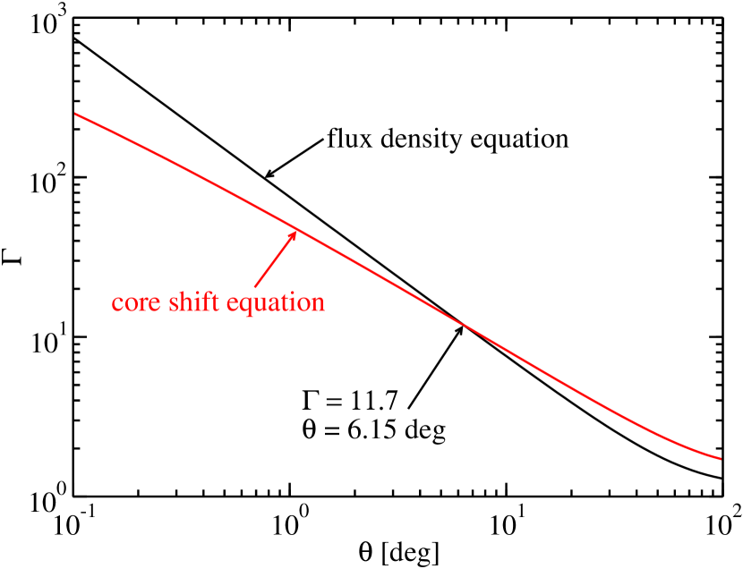
Figure 2.— A plot of $\Gamma$ versus $\theta$ for a particular monte carlo iteration for 2251+158 (3C 454.3) using the core shift equation (Equation [2.7]) and the flux density equation (Equation [2.7]) with the observed parameters given in Table 1. The intersection of these curves gives the numerical solution; in this case, $\Gamma=11.7$ and $\theta=6.15\arcdeg$.

3. Results

3.1. Data

The measurement data taken from the literature can be found in Table 1. The most prominent VLBI instrument is the Very Long Baseline Array (VLBA), spread throughout North America. In general, I rely heavily on data taken as part of the Monitoring of Jets of Active Galactic Nuclei with VLBA Experiments (MOJAVE). I thus use the MOJAVE collaboration’s optical spectral classification for sources (BL Lac object, flat spectrum radio quasar [FSRQ], or Narrow Line Seyfert 1) and redshifts. For a discussion of redshifts and their measurements, particularly BL Lacs that often have unknown or poorly known redshifts, see Lister et al. (2011).

The core shift measurements $\Delta\phi$ from the MOJAVE program between 15 and 8 GHz were taken from Pushkarev et al. (2012). Their errors were taken to be 51 $\mu$as, as discussed by those authors. The core flux densities $F_{\nu}$ at $\nu=15$ GHz were taken from the MOJAVE website (e.g., Lister et al., 2009). The flux densities used were the ones measured during the same epoch the core shift measurement was performed. I assumed there was no error on $F_{\nu}$, since the errors on these values are likely small compared to errors on other observables. Apparent jet opening angles $\alpha_{\rm app}$, measured as part of the MOJAVE program, were taken from Pushkarev et al. (2009). See also Pushkarev et al. (2017). The errors were assumed to be 10%, based on the different results between how the opening angles were measured, in the image plane or in the $(u,v)$ plane, as described by Pushkarev et al. (2009). The extended radio luminosities, $L_{\rm ext}$, are taken from a compilation by Meyer et al. (2011). They found $L_{\rm ext}$ from a spectral decomposition method, separating the core and extended luminosity using spectral energy distribution (SED) shapes. The errors on $L_{\rm ext}$ were also assumed to be negligible.

I found there were 64 sources that were found to have data from all of these sources, including 11 BL Lac objects, 52 FSRQs, and 1 Narrow Line Seyfert 1.

Table 1 Blazar Radio Measurements

Source	Alias	Type	$z$	$\log_{10}\left[\frac{L_{\rm ext}}{\mathrm{erg}\ \mathrm{s}^{-1}}\right]$	$F_{\nu}({\rm core})$ [Jy]	$2\alpha_{\rm app}$ [°]	$\Delta\phi$ [mas]
0133$+$476	DA 55	Q	0.859	41.93	1.781	21.7	0.099
0202$+$149	4C +15.05	Q	0.405	41.39	0.921	16.4	0.113
0212$+$735	S5 0212$+$73	Q	2.367	42.30	3.281	16.4	0.143
0215$+$015	OD 026	Q	1.715	43.52	1.170	36.7	0.111
0234$+$285	4C 28.07	Q	1.207	43.21	2.944	19.8	0.239
0333$+$321	NRAO 140	Q	1.259	42.98	1.343	8.0	0.276
0336$-$019	4C 28.07	Q	0.852	42.36	2.311	26.8	0.105
0403$-$132	PKS 0403$-$13	Q	0.571	43.25	1.808	16.4	0.285
0420$-$014	PKS 0420$-$01	Q	0.914	42.66	3.746	22.7	0.256
0528$+$134	PKS 0528$+$134	Q	2.070	43.73	3.847	16.1	0.150
0605$-$085	OC $-$010	Q	0.872	42.94	1.120	14.0	0.096
0607$-$157	PKS 0607$-$15	Q	0.324	39.84	3.983	35.1	0.254
0716$+$714	S5 0716$+$71	B	0.310	41.98	0.586	17.2	0.125
0738$+$313	OI 363	Q	0.631	42.17	1.226	10.5	0.138
0748$+$126	OI 280	Q	0.889	42.77	3.821	16.2	0.097
0754$+$100	PKS 0754$+$100	B	0.266	41.44	1.304	13.7	0.280
0804$+$499	OJ 508	Q	1.436	42.34	0.458	35.3	0.073
0805$-$077	PKS 0805$-$07	Q	1.837	43.78	1.08	18.8	0.228
0823$+$033	PKS 0823$+$033	B	0.506	40.95	1.828	13.4	0.142
0827$+$243	OJ 248	Q	0.940	42.62	0.775	14.6	0.139
0829$+$046	OJ 049	B	0.174	41.00	0.576	18.7	0.131
0836$+$710	4C +71.07	Q	2.218	43.91	2.222	12.4	0.172
0906$+$015	4C +01.24	Q	1.024	42.67	1.846	17.5	0.203
0917$+$624	OK 630	Q	1.446	43.07	1.017	15.9	0.111
0945$+$408	4C +40.24	Q	1.249	43.64	0.948	14.0	0.113
1038$+$064	4C +06.41	Q	1.265	42.86	1.211	6.7	0.146
1045$-$188	PKS 1045$-$18	Q	0.595	43.19	1.172	8.0	0.167
1101$+$384	Mrk 421	B	0.031	39.59	0.343	18.2	0.254
1127$-$145	PKS 1127$-$14	Q	1.184	43.24	3.308	16.1	0.089
1150$+$812	S5 1150$+$81	Q	1.250	43.44	1.710	15.0	0.082
1156$+$295	4C +29.45	Q	0.729	42.95	3.596	16.7	0.154
1219$+$044	4C +04.42	N	0.965	42.94	1.178	13.0	0.169
1222$+$216	4C +21.35	Q	0.432	42.88	0.507	10.8	0.170
1308$+$326	OP 313	Q	0.997	42.86	0.917	18.5	0.095
1334$-$127	PKS 1335$-$127	Q	0.539	42.51	4.714	12.6	0.274
1413$+$135	PKS B1413$+$135	B	0.247	40.32	0.731	8.8	0.228
1502$+$106	OR 103	Q	1.839	43.30	1.510	37.9	0.056
1504$-$166	PKS 1504$-$167	Q	0.876	42.41	1.162	18.4	0.115
1510$-$089	PKS 1510$-$08	Q	0.360	42.17	1.718	15.2	0.151
1538$+$149	4C +14.60	B	0.605	42.72	1.033	16.1	0.077
1606$+$106	4C +10.45	Q	1.226	42.73	1.462	24.0	0.073
1611$+$343	DA 406	Q	1.397	42.76	4.892	26.9	0.059
1633$+$382	4C +38.41	Q	1.814	43.24	2.419	22.6	0.139
1637$+$574	OS 562	Q	0.751	42.67	1.413	10.7	0.103
1641$+$399	3C 345	Q	0.593	43.16	5.279	12.9	0.201
1652$+$398	Mrk 501	B	0.033	39.46	0.877	19.5	0.279
1730$-$130	NRAO 530	Q	0.902	43.40	2.582	10.4	0.195
1749$+$096	4C +09.57	B	0.322	41.39	4.585	16.8	0.083
1807$+$698	3C 371	B	0.051	40.59	1.137	11.0	0.216
1928$+$738	4C +73.18	Q	0.302	42.28	3.396	9.8	0.155
1936$-$155	PKS 1936$-$15	Q	1.657	42.66	0.691	35.2	0.236
2121$+$053	PKS 2121$+$053	Q	1.941	42.46	1.955	34.0	0.148
2128$-$123	PKS 2128$-$12	Q	0.501	41.90	2.665	5.0	0.242
2131$-$021	4C $−$02.81	Q	1.285	43.33	2.005	18.4	0.099
2134$+$004	PKS 2134+004	Q	1.932	43.51	6.198	15.2	0.172
2155$-$152	PKS 2155$-$152	Q	0.672	42.82	2.151	17.6	0.343
2200$+$420	BL Lac	B	0.069	39.86	3.0	26.2	0.052
2201$+$171	PKS 2201$+$171	Q	1.076	43.05	1.349	13.6	0.369
2201$+$315	4C +31.63	Q	0.295	42.16	2.334	12.8	0.345
2223$-$052	3C 446	Q	1.404	44.11	5.270	11.7	0.162
2227$-$088	PHL 5225	Q	1.560	42.55	1.515	15.8	0.193
2230$+$114	CTA 102	Q	1.037	43.40	2.268	13.3	0.320
2251$+$158	3C 454.3	Q	0.859	43.62	12.541	40.9	0.159
2345$-$167	PKS 2345$-$16	Q	0.576	42.61	2.280	15.8	0.157

3.2. Error Analysis

I determined the values of $\Gamma$ and $\theta$ and their errors from a Monte Carlo (MC) error analysis. For each MC iteration, I randomly drew:

• a core shift, $\Delta\phi$, based on the measured value and assuming a normally distributed error of 51 $\mu$asec.

• an apparent jet opening angle, $\alpha_{\rm app}$, based on the measured value and assuming a normally distributed error of 10% of the measured value.

• values of $c_{1}$ and $c_{2}$ assuming values and normally distributed errors $c_{1}=0.64\pm 0.09$ and $c_{2}=43.54\pm 0.12$ (Cavagnolo et al., 2010). From the randomly drawn $c_{1}$, $c_{2}$, and $L_{\rm ext}$, the jet power $P_{j}$ is calculated from Equation (33).

• values of the nuisance parameters were all drawn from flat priors with limits as follows:

  • $p$ between 1 and 5.

  • $\log_{10}\gamma_{1}$ between 0 and 4.

  • $\log_{10}\gamma_{2}$ between 3 and 7.

  • $\log_{10}\xi_{e}$ between -2 and 2.

  • $\log_{10}\xi_{p}$ between -4 and 2.

  • $\log_{10}\xi_{m}$ between -4 and 2.

If the randomly drawn $\gamma_{2}$ was less than the randomly drawn $\gamma_{1}$, I redrew both parameters. The th parameters $\xi_{p}$ and $\xi_{m}$ were allowed to go much lower than $\xi_{e}$ to include the possibility of an electron-positron jet with few protons, accelerated or otherwise. Note that this marginalizes over the widely-used magnetization parameter,

$$\sigma \equiv\frac{g_{B}\hat{\gamma}_{\rm ad}u_{B}}{u_{e}+u_{p}+\rho c^{2}}$$

$$=\frac{g_{B}\hat{\gamma}_{\rm ad}}{\xi_{e}+\xi_{p}+\hat{\gamma}_{\rm ad}\xi_{m}}\ ,$$ (41)

between $\sigma=0.006$ and $\sigma=200$.

Once all of the parameters are randomly drawn, the values $\Gamma$ and $\theta$ are computed by solving Equations (2.7) and (2.7) numerically. Then other jet parameters, $\alpha$, $B(1\mathrm{pc})$, $\delta_{\rm D}$, and $\beta_{\rm app}$ are computed from these values. This is repeated for $N=10^{4}$ iterations. I compute the magnetic field at $r=1\ \mathrm{pc}$ to be consistent with other calculations of this quantity (e.g., Pushkarev et al., 2012; Zdziarski et al., 2015). The statistical properties of the results can then be computed from these iterations.

3.3. Jet Parameters

The results for two MC calculations can be seen in Figures 3 and 4. Figure 3 shows my result for the famous nearby BL Lac object 1101+384 (Mrk 421). The parameters $\Gamma$ and $\delta_{\rm D}$ are well-constrained to low values, while $\theta$ is poorly constrained. It is interesting to compare the small values of $\Gamma$ and $\delta_{\rm D}$ here with the values inferred from the superluminal components seen in VLBI images (Piner & Edwards, 2004, 2005; Piner et al., 2008, 2010). This is discussed further in Section 4.3. Many of the parameters are well-correlated, such as $\theta$ and $\alpha$, $\theta$ and $B(1\ \mathrm{pc})$, and $B(1\ \mathrm{pc})$ and $\alpha$.

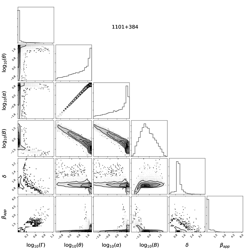
Figure 3.— Result of MC calculation for 1101+384 (Mrk 421). This plot was made with corner.py (Foreman-Mackey, 2016).

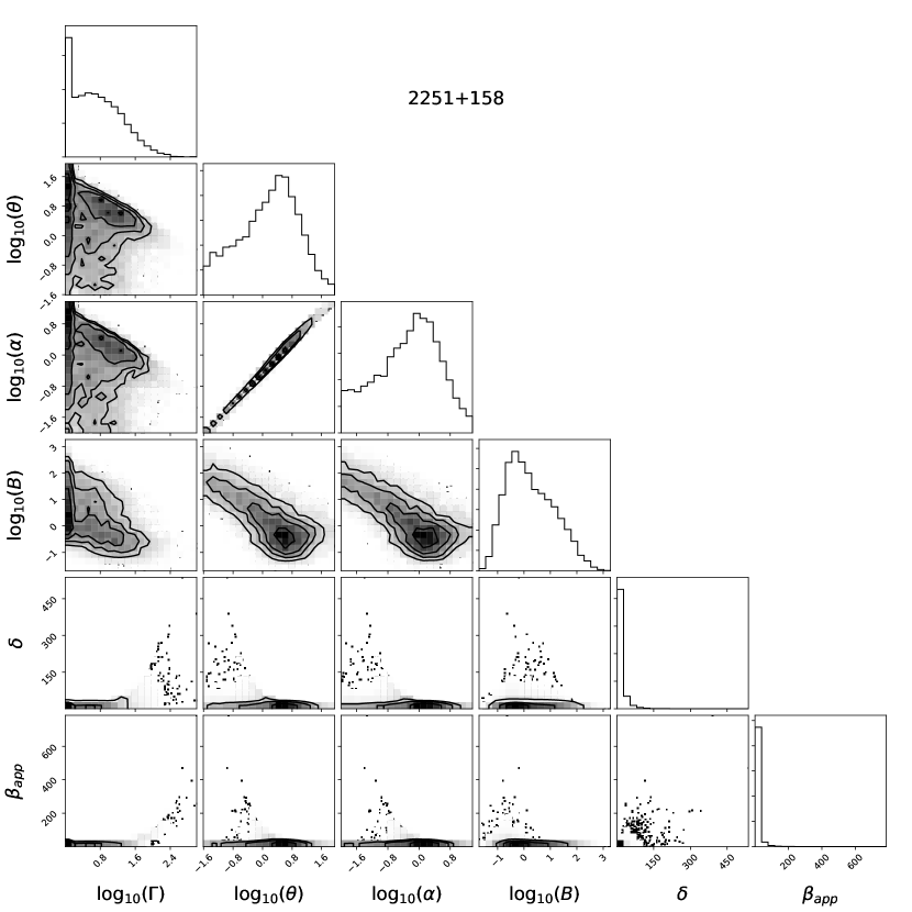
Figure 4.— Result of MC calculation for 2251+158 (3C 454.3). This plot was made with corner.py (Foreman-Mackey, 2016).

Figure 4 shows my result for the famous $\gamma$-ray bright FSRQ 2251+158 (3C 454.3). The angle $\theta$ is much more strongly constrained than for 1101+384, while $\Gamma$ and $\delta_{\rm D}$ are much more poorly constrained. The same parameter correlations seen for 1101+384 are seen for 2251+158 as well, but it is also clear that $\Gamma$ and $\theta$ are well correlated also.

I present the median and 68% confidence intervals of my MC calculation in Table 2. Errors are quite large in many cases, but in some cases parameters are well constrained. For instance, as mentioned above, $\Gamma$ and $\delta_{\rm D}$ are well-constrained for 1101+384. Generally $\delta_{\rm D}$ is well-constrained for low $\delta_{\rm D}$ sources, while $\theta$ is more strongly constrained for higher $\delta_{\rm D}$ sources.

3.4. Alternative Jet Power Calculation

To estimate the jet power of the sources in my sample (Section 2.6), I used the relation between radio lobe luminosity and jet power found by Cavagnolo et al. (2010). This relation was found to be in agreement with the theoretical prediction of Willott et al. (1999) made for Fanaroff-Riley (FR) type II radio galaxies. They used narrow-line luminosities as a proxy for jet power, and found an empirical relation that agreed with their model prediction. Similar empirical correlations have been found for FR I (e.g., Bîrzan et al., 2004, 2008; Cavagnolo et al., 2010; O’Sullivan et al., 2011) and FR II (e.g., Daly et al., 2012) radio galaxies, with authors measuring the jet power in a variety of ways. Agreement between this correlation for FR II and FR I sources was found, contrary to theoretical expectations (Godfrey & Shabala, 2013). Godfrey & Shabala (2016) pointed out that these empirical correlations were probably the result of both the radio luminosity and jet power being dependent on source distance. When taking into account this effect, Ineson et al. (2017) found a correlation

$$\log_{10}\left[\frac{P_{j}}{\mathrm{erg}\ \mathrm{s}^{-1}}\right]=c_{3}\left\{\log_{10}\left[\frac{L_{\rm ext}}{\mathrm{erg}\ \mathrm{s}^{-1}}\right]-44.3\right\}+c_{4}\ ,$$ (42)

with $c_{3}=0.89\pm 0.09$, and $c_{4}=46.7$, in agreement with the theoretical prediction by Willott et al. (1999) for FR II sources.

In Figure 5 I compare my results computed with the relation found by Cavagnolo et al. (2010, Equation (33)) and Ineson et al. (2017, Equation (42)) where in both cases I divide the power by 2 to account for only a single jet. In all cases, the results are within the errors of each other (error bars are not shown on the plot). I conclude that the jet power relation used has little effect on my results.

Table 2Blazar Jet Parameter Results

Source	Alias	$\Gamma$	$\theta$ [°]	$\alpha$ [°]	$B(1\ \mathrm{pc})$ [G]	$\delta_{D}$	$\beta_{\rm app}$
0133$+$476	DA 55	$3.0^{+13.5}_{-1.9}$	$1.7^{+9.7}_{-1.5}$	$0.3^{+1.9}_{-0.3}$	$1.2^{+12.1}_{-1.1}$	$4.8^{+17.0}_{-3.5}$	$0.4^{+9.4}_{-0.4}$
0202$+$149	4C +15.05	$2.3^{+7.1}_{-1.2}$	$5.1^{+20.2}_{-4.6}$	$0.7^{+2.8}_{-0.6}$	$0.5^{+5.6}_{-0.4}$	$3.2^{+7.5}_{-1.9}$	$0.7^{+5.9}_{-0.6}$
0212$+$735	S5 0212$+$73	$3.7^{+15.2}_{-2.7}$	$0.8^{+4.2}_{-0.7}$	$0.1^{+0.6}_{-0.1}$	$4.7^{+26.5}_{-4.3}$	$6.8^{+20.5}_{-5.5}$	$0.3^{+11.0}_{-0.3}$
0215$+$015	OD 026	$2.4^{+7.7}_{-1.3}$	$5.4^{+21.8}_{-5.0}$	$1.7^{+6.7}_{-1.6}$	$0.9^{+13.4}_{-0.7}$	$3.2^{+7.7}_{-1.9}$	$0.8^{+6.1}_{-0.8}$
0234$+$285	4C 28.07	$1.8^{+3.2}_{-0.7}$	$9.4^{+22.8}_{-8.7}$	$1.6^{+3.7}_{-1.5}$	$1.5^{+19.1}_{-1.2}$	$2.3^{+3.1}_{-1.1}$	$0.5^{+3.2}_{-0.5}$
0333$+$321	NRAO 140	$2.2^{+4.3}_{-1.1}$	$13.0^{+24.3}_{-11.0}$	$0.9^{+1.5}_{-0.8}$	$1.5^{+12.0}_{-1.1}$	$2.4^{+3.2}_{-1.2}$	$1.1^{+3.9}_{-1.0}$
0336$-$019	4C 28.07	$3.1^{+12.8}_{-2.0}$	$2.0^{+10.7}_{-1.8}$	$0.5^{+2.5}_{-0.4}$	$1.1^{+12.0}_{-0.9}$	$4.9^{+15.3}_{-3.5}$	$0.6^{+9.2}_{-0.5}$
0403$-$132	PKS 0403$-$13	$1.8^{+2.4}_{-0.7}$	$24.8^{+32.1}_{-22.4}$	$3.4^{+3.5}_{-3.0}$	$0.8^{+8.2}_{-0.5}$	$1.5^{+1.6}_{-0.6}$	$1.0^{+2.0}_{-0.9}$
0420$-$014	PKS 0420$-$01	$1.4^{+1.8}_{-0.3}$	$8.0^{+25.8}_{-7.5}$	$1.6^{+4.8}_{-1.5}$	$1.9^{+25.1}_{-1.7}$	$1.8^{+2.1}_{-0.7}$	$0.1^{+1.9}_{-0.1}$
0528$+$134	PKS 0528$+$134	$9.1^{+35.7}_{-7.2}$	$1.7^{+5.4}_{-1.4}$	$0.2^{+0.8}_{-0.2}$	$1.8^{+13.4}_{-1.3}$	$12.2^{+29.2}_{-9.1}$	$4.3^{+30.6}_{-4.1}$
0605$-$085	OC $-$010	$7.9^{+41.1}_{-6.2}$	$3.1^{+13.0}_{-2.6}$	$0.4^{+1.6}_{-0.3}$	$0.6^{+4.0}_{-0.4}$	$8.2^{+28.9}_{-6.1}$	$4.9^{+31.8}_{-4.5}$
0607$-$157	PKS 0607$-$15	$1.0^{+0.0}_{-0.0}$	$2.8^{+26.3}_{-2.7}$	$0.9^{+7.6}_{-0.8}$	$3.1^{+33.6}_{-2.8}$	$1.0^{+0.2}_{-0.0}$	$0.0^{+0.0}_{-0.0}$
0716$+$714	S5 0716$+$71	$2.4^{+6.0}_{-1.3}$	$13.7^{+30.4}_{-11.8}$	$2.0^{+3.9}_{-1.7}$	$0.3^{+2.3}_{-0.2}$	$2.3^{+4.1}_{-1.2}$	$1.4^{+4.7}_{-1.3}$
0738$+$313	OI 363	$3.9^{+13.2}_{-2.6}$	$5.0^{+15.3}_{-4.2}$	$0.5^{+1.4}_{-0.4}$	$0.7^{+5.8}_{-0.5}$	$4.8^{+10.8}_{-3.2}$	$1.9^{+11.2}_{-1.8}$
0748$+$126	OI 280	$13.4^{+74.6}_{-11.2}$	$1.0^{+4.3}_{-0.8}$	$0.1^{+0.6}_{-0.1}$	$0.9^{+6.2}_{-0.7}$	$18.1^{+66.2}_{-14.6}$	$6.3^{+64.3}_{-6.1}$
0754$+$100	PKS 0754$+$100	$1.2^{+1.0}_{-0.2}$	$22.3^{+37.5}_{-21.2}$	$2.5^{+3.3}_{-2.4}$	$0.6^{+11.2}_{-0.5}$	$1.3^{+0.9}_{-0.3}$	$0.3^{+1.2}_{-0.3}$
0804$+$499	OJ 508	$2.2^{+9.7}_{-1.1}$	$2.8^{+17.2}_{-2.5}$	$0.8^{+5.2}_{-0.8}$	$0.9^{+12.0}_{-0.8}$	$3.2^{+11.9}_{-2.0}$	$0.3^{+6.4}_{-0.3}$
0805$-$077	PKS 0805$-$07	$1.8^{+2.7}_{-0.7}$	$18.4^{+30.8}_{-16.8}$	$2.9^{+4.2}_{-2.6}$	$1.3^{+15.9}_{-1.0}$	$1.8^{+2.1}_{-0.7}$	$0.8^{+2.4}_{-0.8}$
0823$+$033	PKS 0823$+$033	$1.9^{+5.6}_{-0.9}$	$2.4^{+11.6}_{-2.1}$	$0.3^{+1.4}_{-0.2}$	$1.4^{+11.1}_{-1.3}$	$3.1^{+7.3}_{-2.0}$	$0.2^{+4.2}_{-0.2}$
0827$+$243	OJ 248	$2.5^{+6.4}_{-1.3}$	$8.8^{+23.6}_{-7.8}$	$1.1^{+2.9}_{-1.0}$	$0.7^{+7.8}_{-0.5}$	$2.9^{+5.4}_{-1.6}$	$1.1^{+5.4}_{-1.1}$
0829$+$046	OJ 049	$1.8^{+3.3}_{-0.7}$	$14.4^{+31.6}_{-13.1}$	$2.3^{+4.4}_{-2.1}$	$0.2^{+2.7}_{-0.1}$	$1.9^{+2.8}_{-0.8}$	$0.7^{+2.8}_{-0.7}$
0836$+$710	4C +71.07	$7.3^{+25.1}_{-5.5}$	$3.3^{+9.4}_{-2.6}$	$0.4^{+1.0}_{-0.3}$	$1.7^{+11.3}_{-1.2}$	$8.2^{+16.9}_{-5.7}$	$4.3^{+20.8}_{-4.0}$
0906$+$015	4C +01.24	$1.7^{+3.0}_{-0.6}$	$8.9^{+24.2}_{-8.2}$	$1.3^{+3.5}_{-1.2}$	$1.3^{+16.3}_{-1.1}$	$2.2^{+3.1}_{-1.0}$	$0.4^{+2.9}_{-0.4}$
0917$+$624	OK 630	$4.6^{+18.7}_{-3.3}$	$3.8^{+14.6}_{-3.3}$	$0.5^{+2.0}_{-0.4}$	$0.9^{+8.5}_{-0.7}$	$5.6^{+15.9}_{-3.9}$	$2.2^{+15.2}_{-2.1}$
0945$+$408	4C +40.24	$7.2^{+31.7}_{-5.4}$	$4.8^{+16.7}_{-3.9}$	$0.6^{+2.0}_{-0.5}$	$0.8^{+4.0}_{-0.6}$	$6.4^{+18.2}_{-4.5}$	$4.9^{+23.5}_{-4.4}$
1038$+$064	4C +06.41	$8.5^{+32.6}_{-6.6}$	$3.1^{+9.3}_{-2.4}$	$0.2^{+0.5}_{-0.1}$	$1.2^{+6.2}_{-0.9}$	$9.1^{+21.5}_{-6.6}$	$5.6^{+26.4}_{-5.2}$
1045$-$188	PKS 1045$-$18	$7.2^{+23.7}_{-5.2}$	$7.2^{+18.0}_{-5.4}$	$0.5^{+1.2}_{-0.4}$	$0.8^{+2.5}_{-0.5}$	$4.9^{+10.5}_{-3.2}$	$5.2^{+16.0}_{-4.3}$
1101$+$384	Mrk 421	$1.0^{+0.2}_{-0.0}$	$16.3^{+49.3}_{-15.4}$	$2.5^{+5.3}_{-2.4}$	$0.5^{+6.0}_{-0.4}$	$1.1^{+0.2}_{-0.1}$	$0.0^{+0.5}_{-0.0}$
1127$-$145	PKS 1127$-$14	$18.7^{+112.0}_{-16.0}$	$0.9^{+4.4}_{-0.7}$	$0.1^{+0.6}_{-0.1}$	$0.9^{+5.6}_{-0.7}$	$22.6^{+88.0}_{-18.5}$	$10.8^{+93.2}_{-10.4}$
1150$+$812	S5 1150$+$81	$17.1^{+106.5}_{-14.6}$	$1.4^{+7.4}_{-1.2}$	$0.2^{+1.0}_{-0.2}$	$0.8^{+4.2}_{-0.6}$	$17.3^{+72.5}_{-14.0}$	$10.9^{+86.6}_{-10.3}$
1156$+$295	4C +29.45	$5.2^{+17.6}_{-3.8}$	$3.3^{+10.3}_{-2.8}$	$0.5^{+1.5}_{-0.4}$	$0.9^{+8.4}_{-0.7}$	$6.7^{+14.7}_{-4.6}$	$2.3^{+15.0}_{-2.2}$
1219$+$044	4C +04.42	$2.8^{+7.2}_{-1.6}$	$9.1^{+21.7}_{-7.8}$	$1.0^{+2.3}_{-0.9}$	$0.9^{+7.7}_{-0.6}$	$3.1^{+5.5}_{-1.8}$	$1.5^{+6.1}_{-1.3}$
1222$+$216	4C +21.35	$3.1^{+6.7}_{-1.7}$	$20.6^{+31.0}_{-15.5}$	$1.9^{+2.4}_{-1.4}$	$0.5^{+1.5}_{-0.3}$	$1.9^{+2.9}_{-0.9}$	$2.0^{+4.2}_{-1.5}$
1308$+$326	OP 313	$4.6^{+21.6}_{-3.3}$	$4.0^{+17.0}_{-3.5}$	$0.6^{+2.7}_{-0.6}$	$0.6^{+5.7}_{-0.5}$	$5.5^{+17.9}_{-3.8}$	$2.3^{+16.5}_{-2.2}$
1334$-$127	PKS 1335$-$127	$2.4^{+5.2}_{-1.3}$	$7.3^{+16.8}_{-6.4}$	$0.8^{+1.8}_{-0.7}$	$1.1^{+11.7}_{-0.8}$	$3.2^{+4.6}_{-1.8}$	$0.8^{+5.2}_{-0.8}$
1413$+$135	PKS B1413$+$135	$1.2^{+1.1}_{-0.2}$	$15.8^{+34.8}_{-14.6}$	$1.2^{+2.2}_{-1.1}$	$0.6^{+6.9}_{-0.5}$	$1.4^{+1.2}_{-0.3}$	$0.2^{+1.3}_{-0.2}$
1502$+$106	OR 103	$8.6^{+91.1}_{-7.3}$	$0.9^{+7.6}_{-0.7}$	$0.3^{+2.5}_{-0.2}$	$0.8^{+8.8}_{-0.6}$	$12.5^{+96.6}_{-10.6}$	$3.0^{+66.7}_{-3.0}$
1504$-$166	PKS 1504$-$167	$2.9^{+10.0}_{-1.8}$	$4.4^{+17.2}_{-3.9}$	$0.7^{+2.7}_{-0.6}$	$0.8^{+8.7}_{-0.6}$	$4.0^{+10.2}_{-2.6}$	$0.9^{+8.2}_{-0.9}$
1510$-$089	PKS 1510$-$08	$3.2^{+9.1}_{-1.9}$	$7.5^{+20.1}_{-6.4}$	$1.0^{+2.6}_{-0.8}$	$0.4^{+3.9}_{-0.3}$	$3.6^{+7.1}_{-2.2}$	$1.6^{+7.6}_{-1.5}$
1538$+$149	4C +14.60	$10.0^{+65.7}_{-8.1}$	$2.6^{+13.2}_{-2.2}$	$0.4^{+1.8}_{-0.3}$	$0.4^{+2.4}_{-0.3}$	$9.8^{+44.2}_{-7.7}$	$6.3^{+50.1}_{-5.8}$
1606$+$106	4C +10.45	$6.6^{+47.1}_{-5.3}$	$1.3^{+8.7}_{-1.1}$	$0.3^{+1.8}_{-0.2}$	$0.8^{+8.0}_{-0.6}$	$9.3^{+49.7}_{-7.4}$	$2.3^{+35.8}_{-2.3}$
1611$+$343	DA 406	$14.3^{+149.4}_{-12.8}$	$0.4^{+2.7}_{-0.3}$	$0.1^{+0.6}_{-0.1}$	$1.1^{+10.8}_{-0.9}$	$23.1^{+167.2}_{-20.6}$	$3.8^{+121.4}_{-3.8}$
1633$+$382	4C +38.41	$3.4^{+11.6}_{-2.3}$	$2.6^{+10.6}_{-2.3}$	$0.5^{+2.1}_{-0.5}$	$1.7^{+19.2}_{-1.4}$	$5.2^{+12.6}_{-3.6}$	$0.8^{+9.7}_{-0.8}$
1637$+$574	OS 562	$10.2^{+50.5}_{-8.2}$	$2.4^{+9.4}_{-1.9}$	$0.2^{+0.9}_{-0.2}$	$0.7^{+3.8}_{-0.5}$	$10.8^{+35.1}_{-8.2}$	$6.5^{+40.5}_{-6.0}$
1641$+$399	3C 345	$6.7^{+21.4}_{-5.0}$	$3.7^{+9.7}_{-3.0}$	$0.4^{+1.1}_{-0.3}$	$0.9^{+6.3}_{-0.7}$	$7.5^{+13.8}_{-5.1}$	$4.0^{+17.8}_{-3.7}$
1652$+$398	Mrk 501	$1.0^{+0.4}_{-0.0}$	$15.4^{+47.8}_{-14.8}$	$2.5^{+5.8}_{-2.4}$	$0.3^{+6.4}_{-0.3}$	$1.1^{+0.4}_{-0.1}$	$0.0^{+0.8}_{-0.0}$
1730$-$130	NRAO 530	$6.1^{+19.0}_{-4.4}$	$5.1^{+13.0}_{-4.0}$	$0.5^{+1.2}_{-0.4}$	$1.1^{+6.3}_{-0.8}$	$6.0^{+11.4}_{-3.9}$	$4.0^{+14.7}_{-3.6}$
1749$+$096	4C +09.57	$11.7^{+78.2}_{-9.9}$	$0.7^{+3.4}_{-0.5}$	$0.1^{+0.5}_{-0.1}$	$0.5^{+4.0}_{-0.4}$	$17.9^{+80.8}_{-15.0}$	$4.0^{+66.9}_{-4.0}$
1807$+$698	3C 371	$2.5^{+4.8}_{-1.3}$	$19.1^{+29.1}_{-15.1}$	$1.8^{+2.3}_{-1.4}$	$0.1^{+0.6}_{-0.1}$	$2.0^{+2.8}_{-0.9}$	$1.6^{+3.6}_{-1.3}$
1928$+$738	4C +73.18	$10.0^{+38.1}_{-7.8}$	$2.9^{+8.5}_{-2.2}$	$0.2^{+0.7}_{-0.2}$	$0.5^{+2.6}_{-0.3}$	$10.2^{+23.0}_{-7.3}$	$6.8^{+30.4}_{-6.3}$
1936$-$155	PKS 1936$-$15	$1.0^{+0.1}_{-0.0}$	$7.4^{+42.6}_{-7.1}$	$2.3^{+10.8}_{-2.2}$	$7.0^{+111.0}_{-6.4}$	$1.0^{+0.3}_{-0.0}$	$0.0^{+0.2}_{-0.0}$
2121$+$053	PKS 2121$+$053	$1.3^{+2.4}_{-0.3}$	$2.2^{+16.7}_{-2.1}$	$0.7^{+4.8}_{-0.6}$	$3.9^{+38.9}_{-3.6}$	$1.9^{+3.9}_{-0.9}$	$0.0^{+1.3}_{-0.0}$
2128$-$123	PKS 2128$-$12	$5.3^{+15.6}_{-3.8}$	$4.3^{+9.1}_{-3.2}$	$0.2^{+0.4}_{-0.1}$	$1.1^{+6.3}_{-0.8}$	$6.5^{+10.5}_{-4.3}$	$3.0^{+14.1}_{-2.8}$
2131$-$021	4C $−$02.81	$9.0^{+46.6}_{-7.3}$	$1.9^{+8.6}_{-1.6}$	$0.3^{+1.4}_{-0.3}$	$0.9^{+7.2}_{-0.6}$	$10.7^{+38.0}_{-8.2}$	$4.7^{+37.4}_{-4.5}$
2134$+$004	PKS 2134+004	$9.6^{+34.0}_{-7.6}$	$1.3^{+3.6}_{-1.0}$	$0.2^{+0.5}_{-0.1}$	$2.3^{+17.1}_{-1.8}$	$14.0^{+30.6}_{-10.5}$	$3.6^{+31.8}_{-3.5}$
2155$-$152	PKS 2155$-$152	$1.2^{+1.0}_{-0.2}$	$22.9^{+37.3}_{-22.0}$	$3.3^{+4.2}_{-3.2}$	$1.3^{+29.5}_{-1.1}$	$1.3^{+0.9}_{-0.3}$	$0.3^{+1.2}_{-0.3}$
2200$+$420	BL Lac	$10.4^{+118.8}_{-9.0}$	$0.6^{+4.8}_{-0.5}$	$0.1^{+1.1}_{-0.1}$	$0.1^{+1.2}_{-0.1}$	$15.6^{+128.6}_{-13.5}$	$3.2^{+90.7}_{-3.1}$
2201$+$171	PKS 2201$+$171	$1.2^{+1.0}_{-0.2}$	$25.1^{+37.9}_{-24.1}$	$2.8^{+3.1}_{-2.7}$	$2.1^{+44.5}_{-1.7}$	$1.2^{+0.7}_{-0.2}$	$0.2^{+1.1}_{-0.2}$
2201$+$315	4C +31.63	$1.5^{+1.6}_{-0.5}$	$24.6^{+32.0}_{-22.9}$	$2.6^{+2.7}_{-2.4}$	$0.6^{+8.4}_{-0.4}$	$1.5^{+1.3}_{-0.4}$	$0.6^{+1.6}_{-0.6}$
2223$-$052	3C 446	$20.5^{+80.9}_{-16.7}$	$1.5^{+4.5}_{-1.1}$	$0.2^{+0.5}_{-0.1}$	$1.5^{+6.4}_{-1.0}$	$19.6^{+43.1}_{-14.4}$	$14.9^{+62.9}_{-13.7}$
2227$-$088	PHL 5225	$1.6^{+3.1}_{-0.6}$	$5.9^{+19.9}_{-5.4}$	$0.8^{+2.7}_{-0.7}$	$2.2^{+23.7}_{-1.9}$	$2.4^{+3.7}_{-1.2}$	$0.2^{+2.9}_{-0.2}$
2230$+$114	CTA 102	$1.8^{+2.7}_{-0.7}$	$18.7^{+28.9}_{-16.7}$	$2.1^{+2.8}_{-1.9}$	$1.3^{+13.1}_{-1.0}$	$1.8^{+2.0}_{-0.7}$	$0.9^{+2.5}_{-0.8}$
2251$+$158	3C 454.3	$4.8^{+16.1}_{-3.5}$	$1.8^{+7.1}_{-1.7}$	$0.7^{+2.6}_{-0.6}$	$1.3^{+16.2}_{-1.1}$	$7.3^{+16.9}_{-5.2}$	$1.1^{+13.7}_{-1.0}$
2345$-$167	PKS 2345$-$16	$3.5^{+10.4}_{-2.2}$	$5.7^{+16.2}_{-4.9}$	$0.8^{+2.2}_{-0.7}$	$0.7^{+6.5}_{-0.5}$	$4.2^{+8.7}_{-2.7}$	$1.6^{+9.0}_{-1.5}$

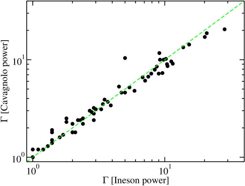
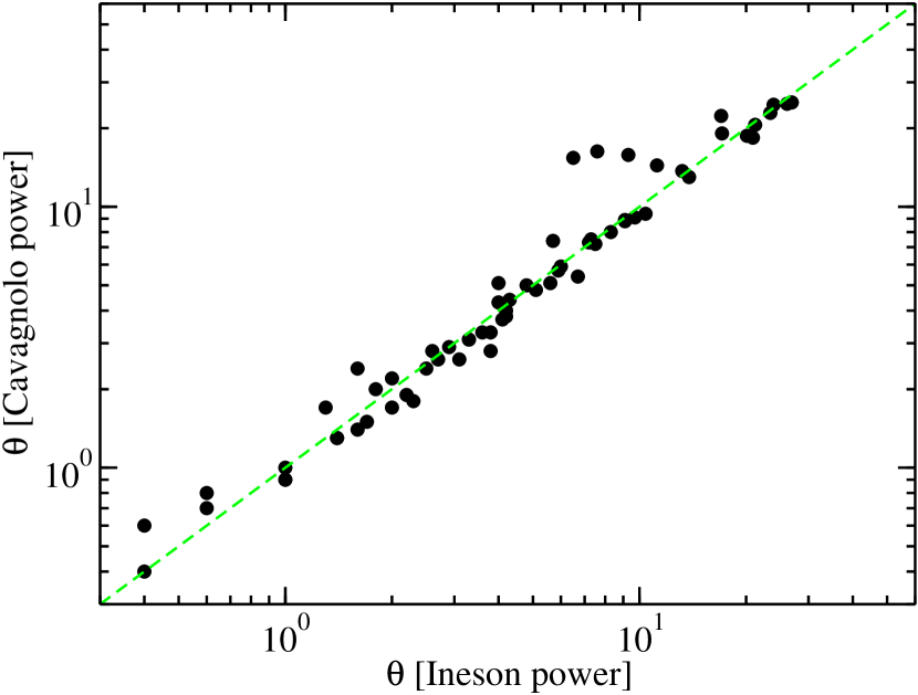
Figure 5.— A comparison of results computed using the relation between $L_{\rm ext}$ and $P_{J}$ found by Cavagnolo et al. (2010, Equation (33)) and Ineson et al. (2017, Equation (42)). Left: A comparison of the bulk Lorentz factor $\Gamma$. Right: A comparison of the angle to the line of sight $\theta$. Error bars are not plotted for clarity. The dashed lines indicates the where the results with the two different calculations are equal.

4. Implications

I explore some implications of my results in this section. I start out by comparing my results with previous calculations of jet parameters (Section 4.1). I then explore what observables could be a good proxy for $\theta$ (Section 4.2), what parsec-scale jet parameters could be related to $\gamma$-ray emission (Section 4.3), and implications for jet physics (Section 4.4). To do this, I test correlations between different parameters and results three different ways. I used the non-parametric Spearman and Kendall rank correlation tests to determine the significance of a correlation between parameters. I also perform linear fits of the form:

$$y=m(x-x_{n})+y_{n}\ .$$ (43)

I performed two fits for each set of variables: with $m$ and $y_{n}$ both as free parameters, and with only $b$ as a free parameter, fixing $m=0$. I then used an F-test to determine the significance of the model with $m$ as a free parameter versus the model with it fixed. The significance of these tests and resulting $m$ and $y_{n}$ from the fits with both as free parameters can be found in Table 3.

4.1. Comparison with Previous Results

Once $\delta_{\rm D}$ and $\theta$ are determined from my method, the apparent speed $\beta_{\rm app}$ one expects can be computed (Equation [40]). This can then be compared with the speeds of knots seen in VLBI jet monitoring programs. The MOJAVE program regularly monitors a number of blazars with the VLBA. On their website they provide the median of the knot apparent speeds when jet speeds for at least 5 knots can be computed. There are 34 objects in my sample that meet this criterion. In Figure 6 I compare my results for $\beta_{\rm app}$ with the median apparent jet speeds from the MOJAVE program. The results are consistent for most sources with in the errors, although my errors are large. For some sources, however, agreement is quite poor. The blazar with the fastest knot in the MOJAVE sample, PKS 0805$-$07 (Lister et al., 2016) actually has a fairly slow core speed based from my determination ($\beta_{\rm app}=2.6^{+4.4}_{-1.7}$), and the median MOJAVE speed is not consistent with my result.

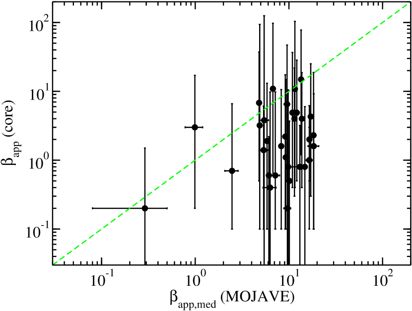
Figure 6.— The apparent jet speed of the core from this work plotted against the median apparent speed of jet components as in VLBI monitoring by the MOJAVE program. The dashed line shows where these two measures are equal.

In Figure 7 I compare my Doppler factor $\delta_{\rm D}$ measurements to the variability Doppler factors measured by Hovatta et al. (2009). Their Doppler factors are computed using radio variability and brightness to determine an observed brightness temperature. This brightness temperature is compared to what one would expect for the maximum intrinsic (unbeamed) brightness temperature if it is limited by equipartition (Readhead, 1994). I plot my Doppler factors against those of Hovatta et al. (2009) in Figure 7. Again, for most sources agreement is within the rather large errors. However, there is some evidence that equipartition may be violated during flares (Homan et al., 2006). Further, the components that flare may have different Doppler factors than the core; knots can accelerate or decelerate (e.g., Homan et al., 2015; Jorstad et al., 2017).

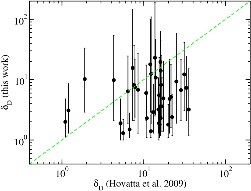
Figure 7.— Variability Doppler factors from Hovatta et al. (2009) compared with this work. Dashed line is where the two methods for determining Doppler factor would be equal.

A different method for determining $\Gamma$, $\theta$, and $\delta_{\rm D}$ for blazar jets was used by Jorstad et al. (2005, 2017). They routinely monitor a number of blazars at 43 GHz with VLBA, and use kinematics of observed knots to determine $\beta_{\rm app}$. The Doppler factors of the individual knots are determined by measuring the timescale for the flux variations and assuming this variability timescale is limited by the size of the knot, which can also be measured from the VLBA images. Once they measure $\beta_{\rm app}$ and $\delta_{\rm D}$ for a knot, they can compute $\theta$ and $\Gamma$. They computed the average jet parameters for all the knots for each source. In Figure 8 I plot the Doppler factors from my calculation versus the average Doppler factors determined by Jorstad et al. (2017) for the sources where our samples overlap. The agreement is clearly quite poor. This could be due to acceleration or deceleration of jet components, or other sorts of variability. The method of determining $\delta_{\rm D}$ from variability used by Jorstad et al. (2005, 2017) assumes the variability timescale is dominated by the light-crossing timescale, which might not be the case.

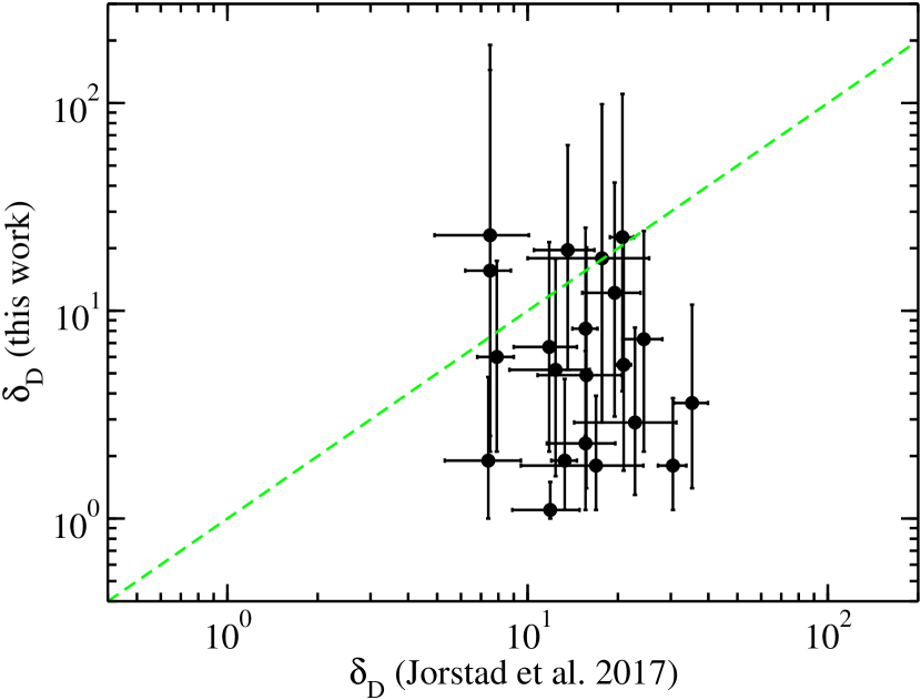
Figure 8.— Doppler factors from Jorstad et al. (2017) compared with this work. Dashed line is the two ways of determining the Doppler factor would be equal.

Using the core shift measurements, and assuming the BK model with $\delta_{\rm D}=\Gamma$ and using the maximum jet speeds from the MOJAVE program, Pushkarev et al. (2012) estimate the magnetic field strength at 1 pc. They also make the assumption of equipartition between electrons and magnetic field ($\xi_{e}=1$ in my notation). In Figure 9 I compare my magnetic field values with theirs. My results are consistent, within the errors, for all sources except one (1334$-$127). This is perhaps not surprising, considering both my calculation and the one of Pushkarev et al. (2012) use the same core shift data, although we make different assumptions. The magnetic field values may pose problems for modeling the multiwavelength SEDs of blazars (Nalewajko et al., 2014).

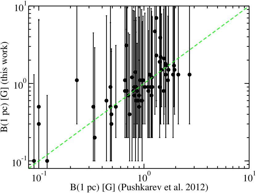
Figure 9.— The magnetic field at 1 pc from this work plotted against the same quantity as measured by Pushkarev et al. (2012). The dashed line shows where these two measures are equal.

4.2. Proxies for Jet Angle

Table 3Correlations results

y	x	Spearman	Kendall	F-test	$m$	$y_{n}$	$x_{n}$
$\log_{10}\Gamma$	$\log_{10}L_{\gamma}$	$1.8\sigma$	$1.9\sigma$	$5.4\sigma$	$0.12\pm 0.03$	$0.21\pm 0.05$	54
$\log_{10}\theta$	$\log_{10}L_{\gamma}$	$2.8\sigma$	$2.8\sigma$	$2.9\sigma$	$-0.18\pm 0.08$	$1.07\pm 0.11$	54
$\log_{10}\alpha$	$\log_{10}L_{\gamma}$	$2.3\sigma$	$2.4\sigma$	$2.6\sigma$	$-0.14\pm 0.07$	$0.19\pm 0.09$	54
$\log_{10}B(1\ \mathrm{pc})$	$\log_{10}L_{\gamma}$	$6.3\sigma$	$>8.3\sigma$	$7.5\sigma$	$0.27\pm 0.14$	$-0.39\pm 0.21$	54
$\log_{10}\delta_{\rm D}$	$\log_{10}L_{\gamma}$	$2.5\sigma$	$2.5\sigma$	$5.4\sigma$	$0.13\pm 0.03$	$0.27\pm 0.04$	54
$\log_{10}\beta_{\rm app}$	$\log_{10}L_{\gamma}$	$1.1\sigma$	$1.1\sigma$	$1.6\sigma$	$0.12\pm 0.11$	$-0.01\pm 0.17$	54
$\log_{10}\theta$	$\log_{10}CD$	$4.5\sigma$	$4.3\sigma$	$5.0\sigma$	$0.67\pm 0.11$	$-0.41\pm 0.18$	2.0
$\log_{10}\theta$	$\Delta\phi$	$6.9\sigma$	$>8.3\sigma$	$6.4\sigma$	$0.32\pm 0.14$	$4.6\pm 1.6$	0.10
$\log_{10}\Phi_{\rm jet}/M_{\rm BH}$	$\log_{10}L_{\rm acc}$	$2.7\sigma$	$2.7\sigma$	$4.3\sigma$	$0.28\pm 0.16$	$33.01\pm 0.28$	47.1
$\log_{10}\theta$	$\log_{10}\nu_{\rm pk}$	$1.5\sigma$	$1.5\sigma$	$1.6\sigma$	$0.36\pm 0.35$	$0.77\pm 0.29$	14
$\log_{10}\theta$	$\log_{10}\nu_{\rm pk}$	$0.9\sigma$	$1.2\sigma$	$1.6\sigma$	$0.27\pm 0.27$	$0.69\pm 0.32$	14

The core dominance (CD)–the ratio of the core to extended radio luminosity–has been used as a proxy for $\theta$ (e.g., Orr & Browne, 1982; Meyer et al., 2011; Marin & Antonucci, 2016). I define CD as the ratio of the core luminosity at 15 GHz (as reported by MOJAVE) to the extended radio luminosity at 300 MHz (as reported by Meyer et al., 2011). The CD as a function of the $\theta$ determined here is plotted in Figure 10. I test whether CD is correlated with $\theta$ and the results are in Table 3. In all cases the significance is $<5\sigma$. Again, I note that my errors on $\theta$ are quite large.

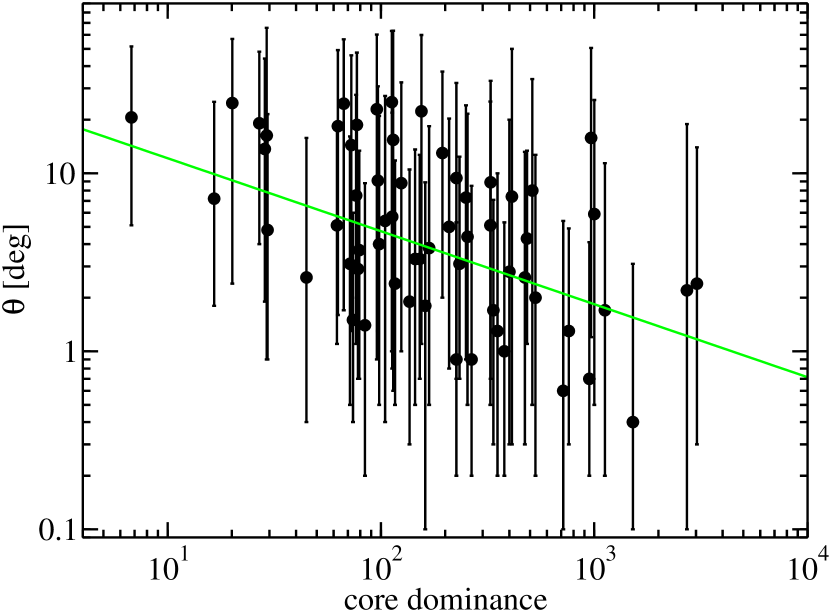
Figure 10.— The result $\theta$ determined here plotted versus CD. The line shows the best fit.

One might also expect the core shift ($\Delta\phi$) to be correlated with $\theta$. I explore this correlation in Figure 11 and Table 3. The viewing angle $\theta$ is much more strongly correlated with $\Delta\phi$ ($>5\sigma$ for all tests) than CD. I conclude that $\Delta\phi$ is a better proxy for $\theta$ than CD. For sources where $\Delta\phi$ is measured, but other measurements needed to use my method are not, my resulting linear fit might be a useful way to estimate $\theta$.

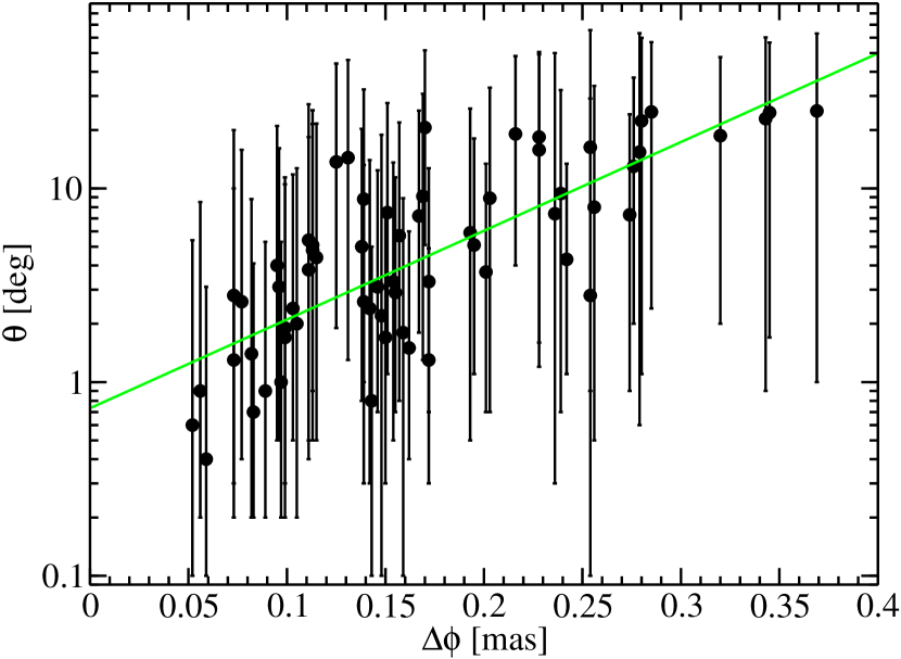
Figure 11.— The result $\theta$ determined here plotted versus $\Delta\phi$. The line shows the best fit.

4.3. Gamma Rays

TeV-detected BL Lac objects are often found to have knots moving at low $\beta_{\rm app}$ indicating low $\Gamma$ and $\delta_{\rm D}$ (Marscher, 1999; Piner & Edwards, 2004, 2005; Piner et al., 2008, 2010). This is in contrast to multiwavelength SED modeling of these sources, which finds much larger values of $\Gamma$ and $\delta_{\rm D}$ (e.g., Finke et al., 2008; Abdo et al., 2011a, b; Inoue & Tanaka, 2016). This discrepancy is sometimes called the “TeV Doppler factor crisis”. For almost every source in my sample $\Gamma\lesssim 4$ is within the quite large 68% confidence interval. Most notably, the two nearest BL Lac objects, Mrk 421 and Mrk 501 have well-constrained low $\Gamma$ and $\delta_{\rm D}$, and sub-luminal implied $\beta_{\rm app}$. Several possible resolutions to the TeV Doppler factor crisis have been suggested: the speed of the jet could be stratified, with a slower layer to explain the low speed from the radio, and a faster spine to explain the multiwavelength emission (Ghisellini et al., 2005). Or the jet could be decelerating, with the faster part closer to the jet explaining the multiwavelength emission and the slower part farther from the jet explaining the radio emission (Georganopoulos & Kazanas, 2003). Finally, the overall flow could have a low $\Gamma$ consistent with radio observations, but magnetic reconnection could lead to the creation of a “jet within a jet” with large $\Gamma$ to explain the multiwavelength emission (Giannios et al., 2009). Mrk 421 and Mrk 501 have values consistent with large angles, but also are consistent with relatively small angles to the line of sight ($\theta>9.9\arcdeg$ and $\theta>4.2\arcdeg$, respectively, at 68% confidence). Large $\theta$ favors the jet within a jet scenario, since in this model the overall jet could be misaligned, but the jet within a jet could be oriented towards the observer. The other explanations require $\theta$ to be small. The small sample and large errors prevent me from making definitive conclusions.

Many blazars are constrained to have low $\delta_{\rm D}$ (Table 2) and are not detected at TeV energies (e.g., PKS 0607$-$15, PKS 1936$-$15). If low $\delta_{\rm D}$ is an indication of brightness at very high energies, these sources could be potential TeV sources, and observation of them with atmospheric Cherenkov telescopes could result in detections. However, many of them are at high redshifts so absorption by the extragalactic background light (e.g., Finke et al., 2010) could make them undetectable.

Although relatively few blazars have been detected with atmospheric Cherenkov telescopes, a much larger number have been detected by the Fermi Large Area Telescope (LAT). Indeed, 54 of the 64 sources in my sample are in the Third LAT AGN Catalog (3LAC; Ackermann et al., 2015). I test correlations between the $\gamma$-ray luminosity from this catalog with all of the parameters presented in Table 2. The results can be seen in Table 3. The strongest correlation is found between $B(1\ \mathrm{pc})$ and $L_{\gamma}$. This result is plotted in Figure 12. This is perhaps not a surprise. The magnetic field $B$ is correlated with $P_{j}$ (Equation [2.6]), which is in turn determined from $L_{\rm ext}$ (Section 2.6). The respective luminosities $L_{\rm ext}$ and $L_{\gamma}$ could be correlated due to both depending on distance. The parameters $\theta$ and $\delta_{\rm D}$ also show strong correlations with the F-test, but not the non-parametric tests.

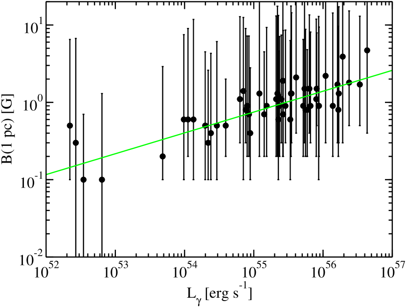
Figure 12.— A plot of $B(1\ \mathrm{pc})$ versus LAT $\gamma$-ray luminosity from the 3LAC. The line shows the best fit.

4.4. Implications for Jet Physics

General relativistic magnetohydrodynamic simulations of jets launched from magnetically arrested disks (MADs) indicate that energy can be extracted from the rotation of black holes to form jets by the Blandford-Znajek mechanism (Blandford & Znajek, 1977) that appear very similar to the ones found in nature (Tchekhovskoy et al., 2011). The parsec-scale magnetic flux $\Phi_{\rm jet}$ can be determined from the jet parameters I have computed by

$$\Phi_{\rm jet}=1.2\times 10^{34}\ \Gamma\alpha\left[\frac{M_{\rm BH}}{10^{9}\ M_{\odot}}\right]\left[\frac{B(1\ \mathrm{pc})}{1\ \mathrm{G}}\right]\ \mathrm{G}\ \mathrm{cm}^{2}$$ (44)

where $M_{\rm BH}$ is the black hole mass, making assumptions about equipartition (Zamaninasab et al., 2014). A more detailed calculation by Zdziarski et al. (2015) gives the more general

$$\Phi_{\rm jet} =8.2\times 10^{33}\ \Gamma\alpha\left[\frac{M_{\rm BH}}{10^{9}\ M_{\odot}}\right]\left[\frac{B(1\ \mathrm{pc})}{1\ \mathrm{G}}\right]\$$ (45)

$$\times\left[\frac{g_{B}\hat{\gamma}_{\rm ad}+\xi_{e}+\xi_{p}+\hat{\gamma}_{\rm ad}\xi_{m}}{\xi_{e}+\xi_{p}+\hat{\gamma}_{\rm ad}\xi_{m}}\right]^{1/2}\mathrm{G}\ \mathrm{cm}^{2}$$

where I have rewritten their result using Equation (3.2). The theory of jets launched from MADs predicts a relationship between $\Phi_{\rm jet}$ and the accretion disk luminosity $L_{\rm acc}$,

$$\Phi_{\rm jet} =2.4\times 10^{34}\left[\frac{M_{\rm BH}}{10^{9}\ M_{\odot}}\right]$$

$$\times\left[\frac{L_{\rm acc}}{1.26\times 10^{47}\ \mathrm{erg}\ \mathrm{s}^{-1}}\right]^{1/2}\ \mathrm{G}\ \mathrm{cm}^{2}$$ (46)

(Zamaninasab et al., 2014). In Figure 13 I plot $\Phi_{\rm jet}/M_{\rm BH}$ determined from Equation (45) using jet parameters from this work versus $L_{\rm acc}$ as found by Zamaninasab et al. (2014). I tested for the significance of the correlation of these quantities (Table 3) and found weak significance with the F-test, and no significance with the Spearman and Kendall tests. As Figure 13 demonstrates, the best fit line does not agree with the model prediction for jets launched from MAD disks from Zamaninasab et al. (2014), which overestimates my results by a factor of $\approx 10$. I have computed $\Phi_{\rm jet}$ for the sources in my sample using both Equation (44) and (45), and the results are not significantly different. Pjanka et al. (2017) compared several estimates of jet power, and found that computing it from extended radio luminosity gives a factor of $\approx 10$ lower result than from core shift measurements or from broadband SED modeling. Since $B_{0}\propto\sqrt{P_{\rm jet}}$ (Equation [2.6]), when I scale up the jet powers by a factor of 10, I find that $\Phi_{\rm jet}$ for my sources increases by a factor of $\approx\sqrt{10}\approx 3$. This improves agreement with Equation (4.4), but the computed results still do not agree with this theoretical curve. The reason for the disagreement is not entirely clear. Equation (45) assumes that all the black holes have spin $a\approx 1$ and Equation (4.4) assumes all accretion disks have an accretion efficiency $\eta=0.4$, neither of which may be the case (Zamaninasab et al., 2014; Zdziarski et al., 2015). Another assumption may not be correct, or these sources may not be accreting in the MAD regime.

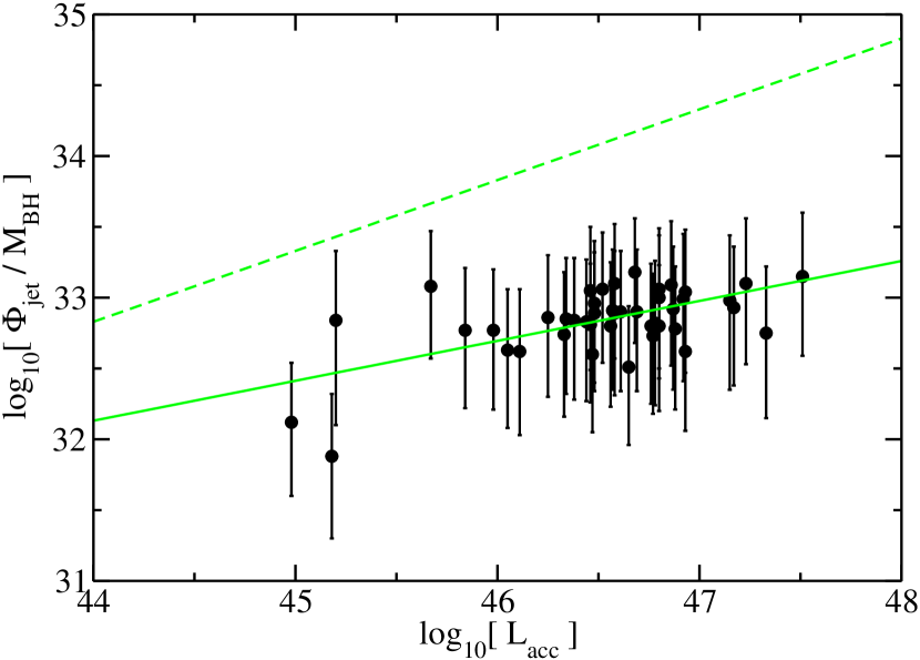
Figure 13.— Correlation between magnetic flux divided by black hole mass ($\Phi_{\rm jet}/M_{\rm BH}$) versus $L_{\rm acc}$. The theoretical expectation from jets launched from a Shakura & Sunyaev (1973) accretion disk around a maximally rotating black hole (Equation [4.4]) is shown as the dashed line while the line from my best fit is shown as the solid line. The parameter $\Phi_{\rm jet}$ is in units $\mathrm{G}\ \mathrm{cm}^{2}$, $M_{\rm BH}$ is in units $10^{9}M_{\odot}$, and $L_{\rm acc}$ is in units $\mathrm{erg}\ \mathrm{s}^{-1}$.

Meyer et al. (2011) have introduced a scenario where FSRQs have jets which essentially have the same $\Gamma$ for the whole jet length, and BL Lac objects have decelerating jets. For BL Lac objects, as $\theta$ increases, one sees slower parts of the jets with larger beaming cones. Their scenario explains the discrepancy between low Doppler factors found in multiwavelength SED modeling of FR I radio galaxies and the high Doppler factors found in modeling the multi-wavelength SEDs of BL Lac objects (e.g., Chiaberge et al., 2000). Their scenario predicts that $\theta$ is correlated with the peak frequency ($\nu_{\rm pk}$) of the low-energy synchrotron component in the SEDs of BL Lac objects. In Figure 14 I plot my determination of $\theta$ versus $\nu_{\rm pk}$ with $\nu_{\rm pk}$ taken from Meyer et al. (2011) and the Third LAT AGN Catalog (3LAC; Ackermann et al., 2015). The correlation between $\theta$ and $\nu_{\rm pk}$ is not significant in any of my tests (Table 3). However, I note that the error on $\theta$ is quite large, and there are only 11 BL Lacs in my sample, and only 2 with $\log_{10}[\nu_{\rm pk}/\mathrm{Hz}]>14.5$. This test is clearly not definitive.

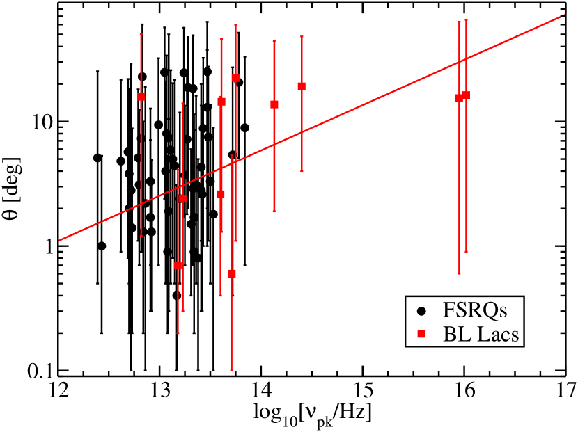
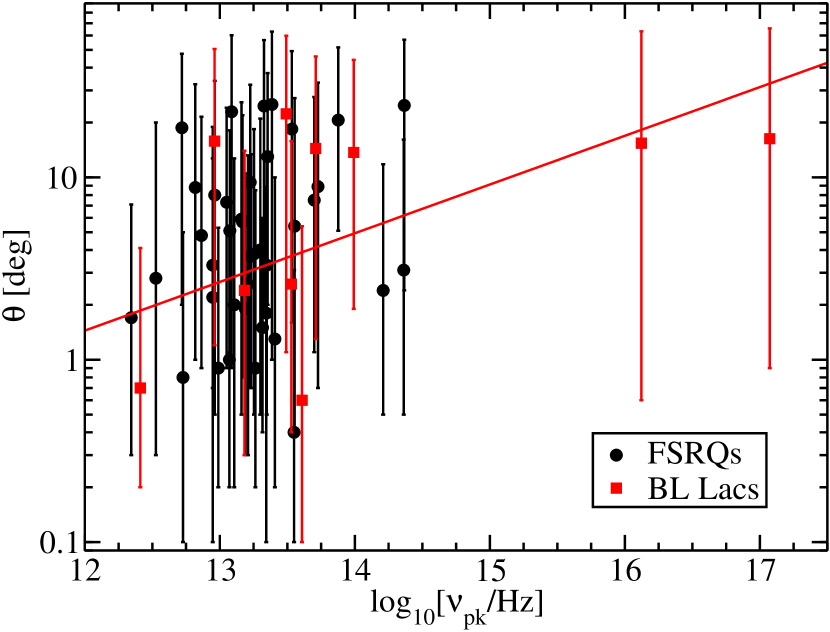
Figure 14.— My determination of $\theta$ versus $\log_{10}\nu_{pk}$ for FSRQs (black circles) and BL Lac objects (red squares). The line indicates the best fit for BL Lac objects. Left: $\log_{10}\nu_{\rm pk}$ from Meyer et al. (2011). Right: $\log_{10}\nu_{\rm pk}$ from 3LAC (Ackermann et al., 2015).

It is expected in the BK model that there is an inverse relationship between the jet Lorentz factor and opening angle, i.e., that $\alpha\Gamma$ is a constant for all sources in the BK jet model. This parameter is important for a number of processes in jet physics (see Clausen-Brown et al., 2013, and references therein). A constant $\alpha\Gamma$ has been found by Jorstad et al. (2005, 2017), Pushkarev et al. (2009, 2017), and Clausen-Brown et al. (2013). I plot $\alpha\Gamma$ for all the sources in my sample in Figure 15. I perform a fit to $\alpha\Gamma=\zeta$ instead of plotting and fitting $\alpha=\zeta/\Gamma$ in order to take into account the correlation in the errors on $\alpha$ and $\Gamma$. I find $\zeta=0.054\pm 0.014$  with $\chi^{2}$/dof = $4.1/63$ , certainly consistent with a constant $\alpha\Gamma$. This value is lower than typically found by other authors. Jorstad et al. (2005) found $\zeta=0.17\pm 0.08$ for their sample, and more recently Jorstad et al. (2017) found $\zeta=0.19\pm 0.07$ and $\zeta=0.32\pm 0.13$ for two different ways of determining $\alpha$. Pushkarev et al. (2009) and Pushkarev et al. (2017) found median $\zeta=0.13$ and $\zeta=0.175$, respectively, in their samples; Clausen-Brown et al. (2013) found $\zeta\approx 0.2$ from their sample.

It is thought that $(\Gamma\alpha)^{2}<\sigma$ (e.g., Tchekhovskoy et al., 2009; Zdziarski et al., 2015; Pjanka et al., 2017). Since, based on my priors, the magnetization parameter, $\sigma$ (Equation [3.2]) ranges from $0.006$ to $200$, and I find $(\Gamma\alpha)^{2}=\zeta^{2}=0.0029\pm 0.0015$, my results indicate that indeed $(\Gamma\alpha)^{2}<\sigma$.

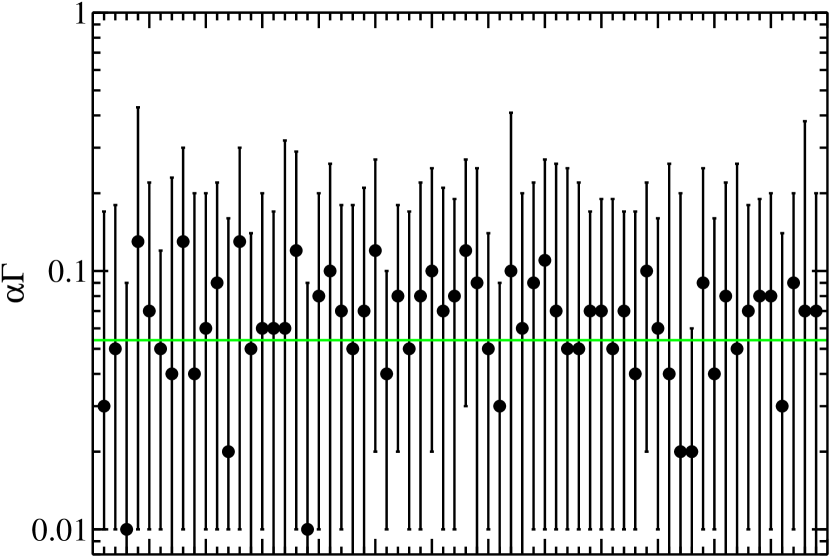
Figure 15.— The value $\Gamma\alpha$ for all sources in my sample. The line shows the best fit value.

5. Discussion

I have shown that using five observables ($z$, $F_{\nu}$, $\Delta\phi$, $\alpha_{\rm app}$, $L_{\rm ext}$) with the BK model, it is possible to determine $\theta$ and $\Gamma$ and other properties for parsec-scale blazar jets. These results are generally consistent with other constraints on $\theta$, $\Gamma$, and $\delta_{\rm D}$, although my errors are quite large. This limits my method’s usefulness. With some exploration, I find that my uncertainties are dominated by two sources:

• The errors on the core shift measurement ($\Delta\phi$) are large, $\approx 15-50\%$. These could be improved by measuring core shifts at multiple frequencies, and doing a fit to these data. Sokolovsky et al. (2011) have done this, although they measure the core shifts with a different technique, and have a much smaller sample size than Pushkarev et al. (2012). Also, there is the issue of validating $\Delta\phi$ measured with different techniques. For instance, for 2201+315, the fit to core shift measurements at 6 frequencies from Sokolovsky et al. (2011) results in $\Delta\phi=0.188\pm 0.009$ masec between 15 and 8 GHz, while Pushkarev et al. (2012) measure a discrepant $\Delta\phi=0.345\pm 0.051$ masec.

• The uncertainty in the electron spectral index ($p$), which I draw from a flat prior. This could in principle be measured from the SEDs of a blazars. However, practically, it is unclear if one could distinguish the parsec-scale portion of the jet from other, more compact, highly variable components that dominate the SED of blazars at high frequencies. Alternatively, one could compute $p$ from $\Gamma$ using shock physics and results from test-particle relativistic shock acceleration theory (Keshet & Waxman, 2005). However, this may not be applicable to realistic shocks, where nonlinear effects could be important. I performed calculations with $p$ constrained by the formula of Keshet & Waxman (2005), and found the resulting $\theta$ for some sources to be unrealistically large. For example, for 1101+384 (Mrk 421) I found $\theta=60^{+10}_{-12}$ deg, inconsistent with the jet/counter-jet brightness ratio constraint for this source (Piner & Edwards, 2005), and the general expectation that blazars have small $\theta$.

It has also been questioned how reliable it is to use the extended radio luminosity as a proxy for jet power (e.g., Godfrey & Shabala, 2016). However, I found that this is not likely to be a major source of error, at least compared to uncertainties on $\Delta\phi$ and $p$ (see Section 3.4). Pjanka et al. (2017) compared several methods of estimating jet power: from extended radio luminosity (the method used here), from core shift measurements, and based on broad-band SED modeling. Each technique has its own set of assumptions. Since authors rarely provide error estimates on jet powers, it is difficult to compare these methods; however, Pjanka et al. (2017) found that the core shift and SED modeling jet powers agreed on average, and that these methods generally gave values $\approx 10$ larger than the extended radio luminosity method. Besides issues with model assumptions, the discrepancy could be due to short term power measured with SED fitting and core shifts, versus long-term power measured with the lobes; or the core shift and SED fitting powers could be lower due to having more electron/positron pairs relative to protons than assumed in these methods (see also Inoue et al., 2017).

Aside from these uncertainties, there is also the problem of variability. At higher frequencies blazars are extremely variable, often with fluxes varying by several orders of magnitude. At radio frequencies, they are less variable, but their fluxes can still vary by $\sim$ a few. The core shifts could also vary with time. I have used measurements of core fluxes and core shifts that are simultaneous. However, since the BK model is an approximation for a variable jet, with a number of colliding shells, there is another source of error associated with the limitations of this model.

Despite these issues I do think this method can be a useful way to constrain jet parameters, complementary to other methods. This will be particularly true if ways to mitigate the uncertainties discussed above can be found.

References

- Abdo et al. (2011a) Abdo, A. A., Ackermann, M., Ajello, M., et al. 2011a, ApJ, 736, 131
- Abdo et al. (2011b) —. 2011b, ApJ, 727, 129
- Ackermann et al. (2015) Ackermann, M., Ajello, M., Atwood, W. B., et al. 2015, ApJ, 810, 14
- Bicknell (1994) Bicknell, G. V. 1994, ApJ, 422, 542
- Bîrzan et al. (2008) Bîrzan, L., McNamara, B. R., Nulsen, P. E. J., Carilli, C. L., & Wise, M. W. 2008, ApJ, 686, 859
- Bîrzan et al. (2004) Bîrzan, L., Rafferty, D. A., McNamara, B. R., Wise, M. W., & Nulsen, P. E. J. 2004, ApJ, 607, 800
- Blandford & Königl (1979) Blandford, R. D., & Königl, A. 1979, ApJ, 232, 34
- Blandford & Znajek (1977) Blandford, R. D., & Znajek, R. L. 1977, MNRAS, 179, 433
- Cavagnolo et al. (2010) Cavagnolo, K. W., McNamara, B. R., Nulsen, P. E. J., et al. 2010, ApJ, 720, 1066
- Chiaberge et al. (2000) Chiaberge, M., Celotti, A., Capetti, A., & Ghisellini, G. 2000, A&A, 358, 104
- Clausen-Brown et al. (2013) Clausen-Brown, E., Savolainen, T., Pushkarev, A. B., Kovalev, Y. Y., & Zensus, J. A. 2013, A&A, 558, A144
- Daly et al. (2012) Daly, R. A., Sprinkle, T. B., O’Dea, C. P., Kharb, P., & Baum, S. A. 2012, MNRAS, 423, 2498
- Dermer & Menon (2009) Dermer, C. D., & Menon, G. 2009, High Energy Radiation from Black Holes: Gamma Rays, Cosmic Rays, and Neutrinos
- Falcke & Biermann (1995) Falcke, H., & Biermann, P. L. 1995, A&A, 293, 665
- Finke et al. (2008) Finke, J. D., Dermer, C. D., & Böttcher, M. 2008, ApJ, 686, 181
- Finke et al. (2010) Finke, J. D., Razzaque, S., & Dermer, C. D. 2010, ApJ, 712, 238
- Foreman-Mackey (2016) Foreman-Mackey, D. 2016, The Journal of Open Source Software, 2016, doi:10.21105/joss.00024
- Georganopoulos & Kazanas (2003) Georganopoulos, M., & Kazanas, D. 2003, ApJ, 594, L27
- Ghisellini et al. (2005) Ghisellini, G., Tavecchio, F., & Chiaberge, M. 2005, A&A, 432, 401
- Giannios et al. (2009) Giannios, D., Uzdensky, D. A., & Begelman, M. C. 2009, MNRAS, 395, L29
- Godfrey & Shabala (2013) Godfrey, L. E. H., & Shabala, S. S. 2013, ApJ, 767, 12
- Godfrey & Shabala (2016) —. 2016, MNRAS, 456, 1172
- Gould (1979) Gould, R. J. 1979, A&A, 76, 306
- Homan et al. (2015) Homan, D. C., Lister, M. L., Kovalev, Y. Y., et al. 2015, ApJ, 798, 134
- Homan et al. (2006) Homan, D. C., Kovalev, Y. Y., Lister, M. L., et al. 2006, ApJ, 642, L115
- Hovatta et al. (2009) Hovatta, T., Valtaoja, E., Tornikoski, M., & Lähteenmäki, A. 2009, A&A, 494, 527
- Ineson et al. (2017) Ineson, J., Croston, J. H., Hardcastle, M. J., & Mingo, B. 2017, MNRAS, 467, 1586
- Inoue et al. (2017) Inoue, Y., Doi, A., Tanaka, Y. T., Sikora, M., & Madejski, G. M. 2017, ApJ, 840, 46
- Inoue & Tanaka (2016) Inoue, Y., & Tanaka, Y. T. 2016, ApJ, 828, 13
- Jamil et al. (2010) Jamil, O., Fender, R. P., & Kaiser, C. R. 2010, MNRAS, 401, 394
- Jorstad et al. (2005) Jorstad, S. G., et al. 2005, AJ, 130, 1418
- Jorstad et al. (2017) Jorstad, S. G., Marscher, A. P., Morozova, D. A., et al. 2017, ApJ, 846, 98
- Keshet & Waxman (2005) Keshet, U., & Waxman, E. 2005, Physical Review Letters, 94, 111102
- Königl (1981) Königl, A. 1981, ApJ, 243, 700
- Kovalev et al. (2008) Kovalev, Y. Y., Lobanov, A. P., Pushkarev, A. B., & Zensus, J. A. 2008, A&A, 483, 759
- Levinson (2006) Levinson, A. 2006, International Journal of Modern Physics A, 21, 6015
- Lister et al. (2009) Lister, M. L., Cohen, M. H., Homan, D. C., et al. 2009, AJ, 138, 1874
- Lister et al. (2011) Lister, M. L., et al. 2011, ApJ, 742, 27
- Lister et al. (2016) Lister, M. L., Aller, M. F., Aller, H. D., et al. 2016, AJ, 152, 12
- Lobanov (1998) Lobanov, A. P. 1998, A&A, 330, 79
- Marin & Antonucci (2016) Marin, F., & Antonucci, R. 2016, ApJ, 830, 82
- Marscher (1999) Marscher, A. P. 1999, Astroparticle Physics, 11, 19
- Meyer et al. (2011) Meyer, E. T., Fossati, G., Georganopoulos, M., & Lister, M. L. 2011, ApJ, 740, 98
- Nalewajko et al. (2014) Nalewajko, K., Begelman, M. C., & Sikora, M. 2014, ApJ, 789, 161
- Orr & Browne (1982) Orr, M. J. L., & Browne, I. W. A. 1982, MNRAS, 200, 1067
- O’Sullivan et al. (2011) O’Sullivan, E., Giacintucci, S., David, L. P., et al. 2011, ApJ, 735, 11
- O’Sullivan & Gabuzda (2009) O’Sullivan, S. P., & Gabuzda, D. C. 2009, MNRAS, 400, 26
- Piner & Edwards (2004) Piner, B. G., & Edwards, P. G. 2004, ApJ, 600, 115
- Piner & Edwards (2005) —. 2005, ApJ, 622, 168
- Piner et al. (2008) Piner, B. G., Pant, N., & Edwards, P. G. 2008, ApJ, 678, 64
- Piner et al. (2010) —. 2010, ApJ, 723, 1150
- Pjanka et al. (2017) Pjanka, P., Zdziarski, A. A., & Sikora, M. 2017, MNRAS, 465, 3506
- Pushkarev et al. (2012) Pushkarev, A. B., Hovatta, T., Kovalev, Y. Y., et al. 2012, A&A, 545, A113
- Pushkarev et al. (2009) Pushkarev, A. B., Kovalev, Y. Y., Lister, M. L., & Savolainen, T. 2009, A&A, 507, L33
- Pushkarev et al. (2017) —. 2017, MNRAS, 468, 4992
- Readhead (1994) Readhead, A. C. S. 1994, ApJ, 426, 51
- Rees (1966) Rees, M. J. 1966, Nature, 211, 468
- Rybicki & Lightman (1979) Rybicki, G. B., & Lightman, A. P. 1979, Radiative Processes in Astrophysics (New York, Wiley-Interscience, 1979. 393 p.)
- Shakura & Sunyaev (1973) Shakura, N. I., & Sunyaev, R. A. 1973, A&A, 24, 337
- Sikora et al. (1997) Sikora, M., Madejski, G., Moderski, R., & Poutanen, J. 1997, ApJ, 484, 108
- Sokolovsky et al. (2011) Sokolovsky, K. V., Kovalev, Y. Y., Pushkarev, A. B., & Lobanov, A. P. 2011, A&A, 532, A38
- Tchekhovskoy et al. (2009) Tchekhovskoy, A., McKinney, J. C., & Narayan, R. 2009, ApJ, 699, 1789
- Tchekhovskoy et al. (2011) Tchekhovskoy, A., Narayan, R., & McKinney, J. C. 2011, MNRAS, 418, L79
- Willott et al. (1999) Willott, C. J., Rawlings, S., Blundell, K. M., & Lacy, M. 1999, MNRAS, 309, 1017
- Zamaninasab et al. (2014) Zamaninasab, M., Clausen-Brown, E., Savolainen, T., & Tchekhovskoy, A. 2014, Nature, 510, 126
- Zdziarski (2014) Zdziarski, A. A. 2014, MNRAS, 445, 1321
- Zdziarski et al. (2012a) Zdziarski, A. A., Lubiński, P., & Sikora, M. 2012a, MNRAS, 423, 663
- Zdziarski et al. (2012b) Zdziarski, A. A., Sikora, M., Dubus, G., et al. 2012b, MNRAS, 421, 2956
- Zdziarski et al. (2015) Zdziarski, A. A., Sikora, M., Pjanka, P., & Tchekhovskoy, A. 2015, MNRAS, 451, 927