Dark matter stripping in galaxy clusters: a look at the Stellar to Halo Mass relation in the Illustris simulation

Abstract

Satellite galaxies in galaxy clusters represent a significant fraction of the global galaxy population. Because of the unusual dense environment of clusters, their evolution is driven by different mechanisms than the ones affecting field or central galaxies. Understanding the different interactions they are subject to, and how they are influenced by them, is therefore an important step towards explaining the global picture of galaxy evolution. In this paper, we use the publicly-available high resolution hydrodynamical simulation Illustris-1 to study satellite galaxies in the three most massive host haloes (with masses $M_{200}>10^{14}\,h^{-1}{\rm M}_{\sun}$) at $z=0$. We measure the Stellar-to-Halo Mass Relation (hereafter SHMR) of the galaxies, and find that for satellites it is shifted towards lower halo masses compared to the SHMR of central galaxies. We provide simple fitting functions for both the central and satellite SHMR. To explain the shift between the two, we follow the satellite galaxies since their time of accretion into the clusters, and quantify the impact of dark matter stripping and star formation. We find that subhaloes start losing their dark matter as soon as they get closer than $\sim 1.5\times R_{\rm{vir}}$ to the centre of their host, and that up to 80% of their dark matter content gets stripped during infall. On the other hand, star formation quenching appears to be delayed, and galaxies continue to form stars for a few Gyr after accretion. The combination of these two effects impacts the ratio of stellar to dark matter mass which varies drastically during infall, from 0.03 to 0.3.

1 Introduction

Clusters of galaxies are the largest gravitationally bound structures in the Universe (Tormen, 1998; Springel et al., 2005; Springel et al., 2001). In the context of the standard hierarchical picture of structure formation processes, clusters are the last structures to form (Lacey & Cole, 1993, 1994; Giocoli et al., 2007). They reside along, and at the nodes of the filamentary network formed by the dark matter density field. In these extremely dense regions, galaxies are subject to violent interactions with their environment, both at the level of dark and baryonic matter, which forces them to follow particular evolutionary paths (Tormen et al., 1998, 2004; Gao et al., 2004; De Lucia et al., 2004).

Many studies show that in the local Universe, galaxies in high density environments are mainly red passive ellipticals (Oemler, 1974; Butcher & Oemler, 1978; Dressler, 1980), and various mechanisms have been identified as having a potential effect on the characteristics of galaxies in clusters: ram-pressure stripping (Gunn & Gott, 1972) can remove the galactic gas and thus quench star formation; frequent encounters with other galaxies, called harassment (Moore et al., 1996; Moore et al., 1998), can disrupt spiral galaxies into ellipticals; mergers in high density environment may favor the survival of massive galaxies (Merritt, 1985; van den Bosch et al., 2005; Conroy et al., 007b); etc. At the same time, interactions of dark matter components also drive the evolution of infalling galaxies (Tormen et al., 2004; Giocoli et al., 2008). Numerical simulations suggest that dynamical friction sinks galaxies towards the center of clusters, with a strength proportional to the mass of the galaxy (Binney & Tremaine, 2008). Concurrently, tidal forces of the host can strip part of the satellite’s matter away, and even disrupt it (Merritt, 1983).

Cosmological simulations offer a privileged tool to follow the evolution of galaxies in “real time” and study the impact of the different interactions they undergo. While progress in computing speed and development of numerical techniques allows now to model the evolution of the Universe under the cold dark matter paradigm, and predicts the structure formation scenario (Springel et al., 2005; Klypin et al., 2011), the life and evolution of galaxies remain more demanding to simulate. Indeed, they depend on many complex baryonic processes acting at different scales. Two main techniques have been developed in the past decade: semi-analytical models (hereafter SAMs) or full hydrodynamical simulations.

SAMs (White & Frenk, 1991; Kauffmann et al., 1993; De Lucia & Blaizot, 2007; Somerville et al., 2008; Guo et al., 2010) rely on dark matter simulations, or on Monte Carlo merger-tree of haloes, populated with seed galaxies. They evolve following analytical prescriptions motivated by models that sit between theory and observations. While this approach has relatively low computational cost and is quite successful at recovering many statistical properties of galaxies such as the stellar mass function (Guo et al., 2015), or the gas fraction (Somerville et al., 2008), it does not directly account for interactions between the baryonic and dark matter components. On the other hand, hydrodynamical simulations (Bonafede et al., 2011; Vogelsberger et al., 2014a; Schaye et al., 2015; De Boni et al., 2018) model the coevolution of dark and baryonic matter by coupling gravity with gas physics, and therefore the dynamical processes are more realistic. They are however much more demanding in terms of computational power, which strongly limits their volume: the largest hydrodynamical simulations such as Illustris (Vogelsberger et al., 2014a) or EAGLE (Schaye et al., 2015), now reach $\sim 100\,\rm{Mpc}$ size, while dark matter only universes have been simulated in boxes with side length of up to a few Gpc (eg. the Big MultiDark simulation, see Klypin et al., 2016).

Here, we want to study the coevolution of dark and baryonic matter. We use the publicly available Illustris simulation , one of the state-of-the art hydrodynamical simulations available today. It includes not only gravitational interactions but also gas dynamics, and some of the most important astrophysical processes, such as gas cooling, stellar evolution and feedback. The runs have been performed with the arepo code (Springel, 2010a). The Illustris simulation was used to study many different aspects of galaxy evolution, such as their formation (Wellons et al., 2015; Martinović & Micic, 2017), structure (Xu et al., 2017) or star formation history (Snyder et al., 2015; Terrazas et al., 2016; Bluck et al., 2016) among others. Here we focus on the evolution of galaxies in clusters, and the evolution of their properties during accretion processes over cosmic time.

Because of this particular environment, satellite galaxies and their subhaloes should evolve differently than central or field galaxies, which in the course of their history are continually growing through accretion of matter and star formation. Conversely, subhaloes will be subject to destructive influence from their host, and their dark matter will be gradually stripped by tidal forces. This effect has been highlighted in a number of analyses of N-body simulations for host haloes ranging from the size of the Milky Way (Hayashi et al., 2003a; Kravtsov et al., 2004; Diemand et al., 2007; Buck et al., 2019) to that of the most massive galaxy clusters (Ghigna et al., 1998; Gao et al., 2004; Tormen et al., 2004; Nagai & Kravtsov, 2005; van den Bosch et al., 2005; Giocoli et al., 2008; Xie & Gao, 2015; Smith et al., 2016; Rhee et al., 2017), where subhalo mass loss is well described by analytical models of tidal stripping (Mamon, 2000; Gan et al., 2010; Han et al., 2016; Hiroshima et al., 2018).

The evolution of the baryonic component has also been widely studied. Observations show an increased proportion of red and passive galaxies in clusters compared to the field. However, the relative importance of the mechanisms that lead to this observation are still being debated. On one hand, violent interactions such as ram-pressure stripping or gravitational interactions, can cause a rapid quenching of the satellite galaxies by removing the cold gas that fuels the formation of new stars (Acreman et al., 2003; George et al., 2013; Bahé & McCarthy, 2015; Boselli et al., 2016; Lotz et al., 2018). On the other hand, some observations favour a slower quenching where the hot gas halo of the galaxies is stripped, preventing their cold gas reservoir from being replenishing. The cold gas is then consumed gradually, which eventually cause the star formation to stop. This slower mechanism is known as ’starvation’ or ’strangulation’ (Wolf et al., 2009; De Lucia et al., 2012; Haines et al., 2015; Zinger et al., 2016; Tollet et al., 2017).

These different evolutionary paths are imprinted notably on the Stellar-to-(sub)Halo Mass Relation (SHMR hereafter). As suggested by gravitational lensing measurements (Limousin et al., 2007; Natarajan et al., 2009; Li et al., 2016; Sifón et al., 2015; Niemiec et al., 2017; Sifón et al., 2018) or measurements calibrated by abundance matching technique (Vale & Ostriker, 2004; Rodríguez-Puebla et al., 2012, 2013), the SHMR of satellite galaxies is shifted towards lower halo masses compared to that of field galaxies. With the advent of large hydrodynamical simulations that allow to self-consistently model the co-evolution of dark and baryonic matter, and thus include any baryonic process that could affect dark matter evolution, some recent studies have re-examined the reason for this shift. Smith et al. (2016) found that the stellar component of cluster galaxies is affected by stripping only when the subhalo has lost a large fraction of its dark matter. In their sample, a vast majority of galaxies do not substantially form stars, and only $18\%$ increase their stellar mass by more than $15\%$ during infall. Using the same set of simulations, Rhee et al. (2017) measured a tight relation between time since infall, tidal mass loss, and position in the phase-space diagram. Finally, Bahé et al. (2017) measured the SHMR for galaxies in the Hydrangea simulation, and observed a shift for galaxies located as far as 5 times the virial radius from the centres of their clusters. They argue that this shift is due to the tidal stripping of subhaloes for galaxies within $2R_{\rm{vir}}$ from the centre of their host, and due to increased star formation for the others.

In this paper, we take advantage of the publicly available simulation Illustris, which combines a very high force and mass resolution with a relatively large cosmological volume, in order to push further our understanding of galaxy evolution in clusters. We measure the shift between the SHMRs of central and satellite galaxies, and examine the mechanisms that may cause this difference. This is done for both dark and baryonic matter. We quantify their relative importance as well as the time scales over which they operate.

This paper is organized as follows: Sect. 2 presents the data from the Illustris simulation we use; Sect. 3 details our measurements of the SHMR for the simulated galaxies (both centrals and satellites), and presents the best fitting models for the relation in both cases; Sect. 4 discusses the evolution of galaxies during infall, making use of the merger trees for all subhaloes in cluster-like host-halos; Sect. 5 presents the quantification of the stripping of halos as a function of their distance to the cluster centre; Sect. 6 summarizes our results, and discusses them in a wider context. The cosmology used throughout this paper is identical to that used in the Illustris simulation, a flat $\Lambda$CDM universe consistent with the Wilkinson Microwave Anisotropy Probe 9-year data release (WMAP9, Hinshaw et al., 2013, : $\Omega_{\rm{m,0}}=0.2726$, $\Omega_{\Lambda,0}=0.7274$, $\Omega_{\rm{b,0}}=0.0456$, $\sigma_{8}=0.809,n_{\mathrm{s}}=0.963$ and $H_{0}=70.4\rm{km\,s}^{-1}$). The notation log() refers to the base 10 logarithm.

2 Data

2.1 The Illustris simulation

In this analysis we use the publicly-available data from the Illustris simulation, more specifically the group catalogues and merger trees. We summarize in this section the simulation details and refer to the corresponding publications.

Simulation details.

Illustris is a hydrodynamical simulation (Vogelsberger et al., 2014b, a) in which dark matter and gas dynamics evolve simultaneously, using the moving-mesh code arepo (Springel, 2010b), from initial conditions following a $\Lambda$CDM cosmology with WMAP-9 parameters (Hinshaw et al., 2013) starting at redshift $z=127$, in a comoving box with a side of $75\,h^{-1}\mathrm{Mpc}=106.5\,\mathrm{Mpc}$. The simulation includes astrophysical processes to drive galaxy evolution, including gravity, gas cooling and heating, stellar formation and evolution, feedback from stars, and supermassive black holes.

Three simulations were run with different resolutions: Illustris-1 (dark matter particle $m_{\mathrm{DM}}=4.41\times 10^{6}\,h^{-1}{\rm M}_{\sun}$, baryonic particle $m_{\mathrm{b}}=8.86\times 10^{5}\,h^{-1}{\rm M}_{\sun}$); Illustris-2 ($m_{\mathrm{DM}}=3.53\times 10^{7}\,h^{-1}{\rm M}_{\sun}$, $m_{\mathrm{b}}=7.09\times 10^{6}\,h^{-1}{\rm M}_{\sun}$); and Illustris-3 ($m_{\mathrm{DM}}=2.82\times 10^{8}\,h^{-1}{\rm M}_{\sun}$, $m_{\mathrm{b}}=5.67\times 10^{7}\,h^{-1}{\rm M}_{\sun}$). The work presented in this paper is based on the highest resolution run, Illustris-1. The simulation is sampled in 136 snapshots from $z=127$ to $z=0$. Groups were detected by the Illustris collaboration with a Friends-of-Friends (FoF) algorithm with linking length $b=0.2$ , and the haloes were extracted using the subfind algorithm (Springel et al., 2001; Dolag et al., 2009), and classified into centrals and satellites from their ranking within their FoF group. Thus, the central halo is generally the most massive subhalo in the group. The snapshot at $z=0$ contains $4,366,546$ subfind groups.

Merger trees.

Merger trees were constructed by (Rodriguez-Gomez et al., 2015) for the simulation using two different codes, SubLink and LHaloTree (Springel et al., 2005). We chose the SubLink merger trees for our analysis. They created the trees as follow. At each time step, a descendant is identified for each subhalo, based on the number of common particles and their binding energy. To avoid losing low mass subhaloes when they cross a structure, SubLink allows for one snapshot to be skipped when it looks for descendants. Once all the descendant connections are established the main progenitor of each subhalo is defined as the one with the most massive history behind it.

2.2 Cluster haloes and their subhaloes in the Illustris simulation

In this section we describe the haloes and subhaloes from the Illustris-1 simulation that are used in this work. As described above, the Illustris-1 simulation is the most resolved run, with dark matter particle mass $m_{\mathrm{DM}}=6.3\times 10^{6}\,{\rm M}_{\sun}$ and effective baryonic resolution $m_{\mathrm{b}}=1.3\times 10^{6}\,{\rm M}_{\sun}$. We select the three most massive systems in the simulation, with a mass $M_{200}>10^{14}\,h^{-1}{\rm M}_{\sun}$ at $z=0$ – where $M_{200}$ refers to the mass enclosing $200$ times the critical density of the universe $\rho_{c}$, with $R_{200}$ the corresponding radius. This mass selection is equivalent to the redMaPPer cluster selection with richness $\lambda>20$ (Rykoff et al., 2014; Rozo & Rykoff, 2014). We present in Table 1 the main properties of these haloes at the two redshifts of interest, $z=0$ and $z=0.35$, where the latter is the mean redshift of the redMaPPer-SDSS clusters, used to compare our results to observations (e.g Li et al., 2016; Niemiec et al., 2017). In the next section we compare the SHMR measured for satellite galaxies of these three host haloes to the one measured for all central galaxies of the simulation (142,720 centrals at $z=0$ with $M_{*}>0$).

The top panel of Fig. 1 shows the mass evolution of the three haloes from $z=1$ to $z=0$. One can see that Halo 1 has undergone some violent mass changes in recent times due to a major merger event. Looking at the mass history of the most massive subhaloes in Halo 1, a recent merger of three haloes of mass $\sim 1-5\times 10^{13}\,h^{-1}{\rm M}_{\sun}$ is indeed identified within the redshift range z=0-0.4. It is therefore possible that the subbaloes of Halo 1 experience a different evolution than the subhaloes of Halo 0 and Halo 2. In the top panel of Fig. 1, the dashed line shows the average mass accretion history predicted from the model presented by Giocoli et al. (2012); Giocoli et al. (2013). This relation is consistent with the measured evolution of Halo 0 and Halo 2, which have experienced a smoother evolution since $z=1$ than Halo 1.

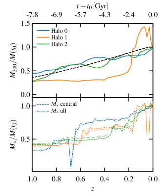
Figure 1: Mass accretion history of the three most massive haloes in the Illustris-1 simulation, showing $M_{200}$ in the top panel, and the stellar mass in the bottom panel defined as the central galaxy stellar mass (dashed line), and the mass of all stellar particles in the halo, excluding the subhaloes (dotted line). The recent drastic mass changes in the accretion history of Halo 1 suggest that it is undergoing a major merger. We show in addition as the black dashed line in the top panel, the average mass accretion history for a halo with $M_{200}(z=0)=10^{14}h^{-1}{\rm M}_{\sun}$ as predicted from the model presented by Giocoli et al. (2012); Giocoli et al. (2013).

	$z=0$				$z=0.35$
Halo ID	$\log M_{200}/h^{-1}{\rm M}_{\sun}$	$\log M_{*}/h^{-1}{\rm M}_{\sun}$	$N_{\mathrm{subs}}$	$N_{\mathrm{sub}}^{*}$	$\log M_{200}/h^{-1}{\rm M}_{\sun}$	$\log M_{*}/h^{-1}{\rm M}_{\sun}$	$N_{\mathrm{subs}}$	$N_{\mathrm{subs}}^{*}$
0	14.21	12.18	5070	120	14.08	12.08	4113	97
1	14.20	11.99	6756	138	13.76	11.81	1855	33
2	14.19	12.13	5262	112	14.05	11.89	4268	85

Table 1: Properties of the three most massive haloes in the Illustris simulation: mass $M_{200}$, stellar mass of the central galaxy $M_{*}$ defined as the sum of all star particles within twice the stellar half mass radius, the total number of subhaloes $N_{\mathrm{sub}}$, and the number of subhaloes with $M_{\mathrm{sub}}>10^{10}\,h^{-1}{\rm M}_{\sun}$ $N_{\mathrm{sub}}^{*}$.

Different estimates of the mass are available for the various objects in the simulation. Following Vogelsberger et al. (2014a), we use galaxy properties defined within twice the stellar half-mass radius. The stellar mass is therefore the sum of the mass of all star particles within this radius. We define stellar mass in the central haloes as the stellar mass in the central galaxy (another definition could be the sum of all star particle in the halo excluding the subhaloes; we show the stellar mass accretion history for these two definitions in the bottom panel of Fig. 1). Fig. 2 shows the Stellar Mass Function (SMF) of all the central galaxies in the simulation (solid line), and of the satellite galaxies of the three host haloes described above (dashed line), at $z=0$ (blue) and $z=0.35$ (orange). One can see that while the satellite SMF increases by $\sim 0.5$ dex between $z=0.35$ and $z=0$, the central SMF does not evolve significantly.

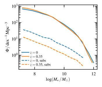
Figure 2: Stellar mass function for all the central galaxies in the Illustris-1 simulation (solid line), and the satellite galaxies of the three most massive haloes (dashed line), at $z=0$ (blue) and $z=0.35$ (orange.)

We remind the reader that for the dark matter content, central haloes are defined as spherical regions with a radius $R_{200}$, with an average density equal to 200 times the critical density of the Universe, $\rho_{\mathrm{c}}(z)$. The mass of the central halo is the total mass enclosed in this region, $M_{200}$. For the subhaloes, where this definition does not apply, the mass is defined as the sum of the masses of all particles identified as being gravitationally bound to the subhalo (Springel et al., 2001; Gao et al., 2004; Giocoli et al., 2008, 2010).

3 Stellar-to halo mass relation of haloes and subhaloes

3.1 SHMR for central haloes

We now focus on the stellar-to-halo mass relation (SHMR). We first look at the relation for central haloes. This will be used as our reference for the comparison with subhaloes. The relation is shown in Fig. 3. The blue open circles mark the SHMR for each (central) halo of the simulation, and in black points we plot the median relation in five bins of stellar mass: $10^{7}<M_{*}<10^{8}$, $10^{8}<M_{*}<10^{9}$, $10^{9}<M_{*}<10^{10}$, $10^{10}<M_{*}<10^{11}$ and $10^{11}<M_{*}<10^{12}$, in units of $h^{-1}{\rm M}_{\sun}$, where the small error bars represent the 1$\sigma$ uncertainty on the median. Comparing the two panels, we do not notice a strong evolution between redshift $z=0$ and $z=0.35$, in agreement with the SMF described above, which shows that stars and dark matter evolve together.

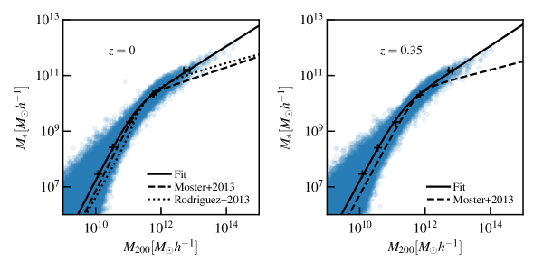
Figure 3: Stellar-to-halo mass relation for haloes from the Illustris-1 simulation. The left and right panels show the measurements at redshift $z=0$ and $z=0.35$, respectively. The masses are expressed in units of $h^{-1}{\rm M}_{\sun}$. Blue open circles represent the SHMR for each central halo of the simulation. The black points are median values in bins of stellar mass. The error bars represent the $1\sigma$ uncertainty on the median. In addition, we plot the relation computed from abundance matching in Moster et al. (2013) at the two redshifts (dashed line), and in Rodríguez-Puebla et al. (2013) for $z=0$ only (dotted line). The black solid lines represent the best-fit relation.

In addition, we show the stellar-to-halo mass relation obtained from abundance matching in Moster et al. (2013), defined as:

$$\frac{M_{*}}{M_{200}}=2N\left[\left(\frac{M_{200}}{M_{1}}\right)^{-\beta}+\left(\frac{M_{200}}{M_{1}}\right)^{\gamma}\right]^{-1}$$ (1)

, where the best fit parameters from Moster et al. (2013) at $z=0$ are $\log(M_{1}/{\rm M}_{\sun})=(11.590\pm 0.236)$, $N=(0.0351\pm 0.0058)$, $\beta=(1.376\pm 0.153)$ and $\gamma=(0.068\pm 0.059)$ (the redshift dependence of the parameters is given in Moster et al., 2013). We also plot the relation obtained with abundance matching in Rodríguez-Puebla et al. (2013) for central galaxies (we use their results from set C).

These two SHMR differ from our measurements at the two mass extrema. This discrepancy is due to shortcomings in both calculations. It has been shown (Sawala et al., 2013; Munshi et al., 2013) that SHMR estimated from dark matter only simulations (as in Moster et al., 2013) overestimates the mass of dark matter haloes, especially at low masses, due to the lack of baryonic physics. However, when correcting for this difference by matching the subhaloes to their counterpart in Illustris DM-only run, the Illustris simulation still appears to overpredict the stellar masses of the most and least massive haloes (Genel et al., 2014; Vogelsberger et al., 2014a). At the high mass end, the prediction of overly massive galaxies could be due to insufficient AGN feedback in the Illustris samples (eg. Vogelsberger et al., 2014a). At intermediate mass scales, $M_{*}\sim 10^{9}-10^{11}\,h^{-1}{\rm M}_{\sun}$, the measurements are in good agreement.

We fit the parameters $M_{1}$, $N$, $\beta$ and $\gamma$ from equation 1 to the measured SHMR at $z=0$ and $z=0.35$. As our galaxy sample is dominated by low-mass objects, we need to weight their contribution. We therefore split the galaxies into 15 bins in $\log M_{*}$, and perform fit the median values in each bin, with the standard deviation of $\log M_{*}$ in each bin as the error estimate. We obtain the best-fit parameters and the intervals of confidence with a Markov Chain Monte Carlo (MCMC) method using emcee (Foreman-Mackey et al., 2013), which is a Python implementation of an affine invariant MCMC ensemble sampler. The best-fit parameters and the 68% credible intervals are presented in Table 2. We also present the joint 2-dimensional, and marginalized 1-dimensional posterior probability distributions for the parameters $M_{1}$, $N$, $\beta$ and $\gamma$ at $z=0$ in Appendix A. The “normalization” parameters $M_{1}$, and $N$, are in reasonable agreement with Moster et al. (2013), but as expected the slopes are different, steeper at high mass and flatter at low mass. The solid black curve shows the SHMR corresponding to our best-fit parameters in Fig. 3. To compare our measurements with Moster et al. (2013), we let our best-fit SHMR parameters evolve bewtween $z=0$ and $z=0.35$ using the redshift parametrization described in equations (11) - (14), and Table 1 from Moster et al. (2013). The values are shown in Table 2. We measure a weaker redshift evolution (consistent with no evolution) than what Moster et al. (2013) predicts.

Haloes
	Fit $z=0$	Fit $z=0.35$	Evolved
$\log M_{1}/h^{-1}{\rm M}_{\sun}$	$11.21^{+0.18}_{-0.17}$	$11.26^{+0.20}_{-0.20}$	$11.52$
$N$	$0.030^{+0.007}_{-0.006}$	$0.025^{+0.006}_{-0.006}$	$0.024$
$\beta$	$1.27^{+0.13}_{-0.11}$	$1.17^{+0.13}_{-0.11}$	$1.06$
$\gamma$	$0.26^{+0.08}_{-0.08}$	$0.23^{+0.09}_{-0.08}$	$0.35$
Subhaloes
	Fit $z=0$	Fit $z=0.35$	Evolved
$\log M_{1}/h^{-1}{\rm M}_{\sun}$	$10.66^{+0.35}_{-0.26}$	$10.67^{+0.31}_{-0.24}$	$10.97$
$N$	$0.091^{+0.034}_{-0.021}$	$0.099^{+0.033}_{-0.020}$	$0.084$
$\beta$	$0.98^{+0.13}_{-0.12}$	$0.95^{+0.11}_{-0.11}$	$0.78$
$\gamma$	$0.16^{+0.17}_{-0.09}$	$0.09^{+0.14}_{-0.06}$	$0.25$

Table 2: Best-fit parameters and $68\%$ credible intervals for the parameters $M_{1}$, $N$, $\beta$ and $\gamma$ from equation 1 fitted to the haloes and subhaloes at $z=0$ and $z=0.35$. We assumed flat priors such as: $\log M_{1}/h^{-1}{\rm M}_{\sun}\in[10.5;12.5]$, $N\in[0;2]$, $\beta\in[0;5]$ and $\gamma\in[0;5]$. We also present the value of the $z=0$ best fit parameters evolved to $z=0.35$ using the redshift parametrization from Moster et al. (2013).

3.2 SHMR for subhaloes

We now plot the SHMR for subhaloes in the three cluster-like haloes described in Sect. 2.2. We consider all subhaloes in the subfind catalogues, except for the first one as it is the central halo. Figure 4 shows the relation for individual subhaloes, in stellar mass bins, similarly to the SHMR for central halos.

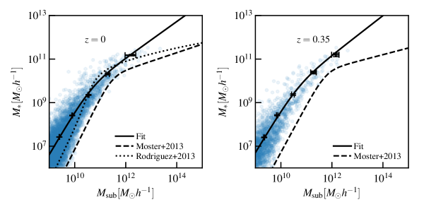
Figure 4: Stellar-to-halo mass relation for subhaloes of the “cluster like” haloes from the Illustris-1 simulation. Left and right panels shows our measurements at $z=0$, and $z=0.35$ respectively. In addition, we plot our best-fit relations at $z=0$ and $z=0.35$ (solid line). For comparison, we show the same relation as in Fig. 3, computed from simulations in Moster et al. (2013) (dashed line). The relation for subhaloes appears to be shifted towards lower dark matter mass compared to the one for haloes. We also display the relation from Rodríguez-Puebla et al. (2013) at $z=0$, measured by abundance matching for satellite galaxies and their subhaloes (dotted line).

Figure 4 shows that the SHMR is shifted towards lower halo masses for subhaloes compared to central haloes. In Table 3, we list the stellar and halo masses for each bin, for both central and satellite populations. The error bars represent the standard errors. We fit again the parameters $M_{1}$, $N$, $\beta$ and $\gamma$ from equation 1 using the same procedure as for centrals. The best fit values and the $68\%$ credible intervals at $z=0$ and $z=0.35$ are listed in Table 2. The posterior probability distributions at $z=0$ are given in Appendix A. The solid line in Fig. 4 shows the relation constructed using the best fit parameters. In Table 2, we also list the best fit parameters at $z=0$ evolved to $z=0.35$, adopting the Moster et al. (2013) redshift parametrization. As in the case of central galaxies, our measurements show a weaker redshift evolution than Moster et al. (2013).

The dotted line in Fig. 4 shows the SHMR for satellite galaxies measured by abundance matching in Rodríguez-Puebla et al. (2013). The shift of this relation compared to central galaxies is similar to our measurement at intermediate mass scale ($M_{*}\sim 10^{9}-10^{11}\,h^{-1}{\rm M}_{\sun}$), but the slopes differ at both mass ends.

Finally, considering the assumption that the stellar mass does not evolve during accretion, and that the “progenitors” of subhaloes at a given stellar mass are central haloes of same stellar mass, we define the stripping factor as

$$\tau_{\mathrm{strip}}(M_{*})=1-\frac{M_{\mathrm{sub}}(M_{*})}{M_{\mathrm{h}}(M_{*})}\mathrm{,}$$ (2)

and present the results for each stellar mass bin in Table 3. From this perspective, the stripping factor simply represents the shift in halo mass of the SHMR between central haloes and subhaloes. Fig. 5 shows the evolution of the stripping factor as a function of the mean stellar mass in each bin for $z=0$ and $z=0.35$. There is no significant evolution with the stellar mass nor the redshift. In addition, we plot the mean value of the stripping factor $\langle\tau_{\rm strip}\rangle=0.75$, and find no significant deviation from it. We compare our results with those obtained by Rodríguez-Puebla et al. (2013) using abundance-matching by computing $\tau_{\rm{strip}}$ from their SHMR for satellite and central galaxies. Although they find a mass dependence for the stripping factor, it is small in the mass range that we consider, and we consider our results to be in good agreement. We also note that the relation from Rodríguez-Puebla et al. (2013) was calibrated using dark matter-only simulations, where the impact of baryons on halo formation history is not taken into account. This could explain the small difference that we observe at the low mass end. Finally we checked that defining the mass of the central haloes as the sum of the masses of all gravitationally bound particles $M_{\mathrm{bound}}$, in order to use the same dark matter mass definition as for subhaloes, or using $M_{*\mathrm{,bound}}$ for both haloes and subhaloes, does not change our conclusions.

	$z=0$
$M_{*}$ bin	$M_{200}\times 10^{-11}$	$M_{\mathrm{sub}}\times 10^{-11}$	$\tau_{\mathrm{strip}}$
($h^{-1}{\rm M}_{\sun}$)	($h^{-1}{\rm M}_{\sun}$)	($h^{-1}{\rm M}_{\sun}$)
$10^{7}-10^{8}$	$0.119\pm 0.001$	$0.025\pm 0.001$	$0.79\pm 0.02$
$10^{8}-10^{9}$	$0.331\pm 0.001$	$0.080\pm 0.003$	$0.76\pm 0.03$
$10^{9}-10^{10}$	$1.10\pm 0.01$	$0.347\pm 0.020$	$0.69\pm 0.05$
$10^{10}-10^{11}$	$5.83\pm 0.21$	$1.98\pm 0.37$	$0.66\pm 0.15$
$10^{11}-10^{12}$	$62.4\pm 13$	$17.1\pm 9.6$	$0.73\pm 0.56$
	$z=0.35$
$10^{7}-10^{8}$	$0.121\pm 0.001$	$0.022\pm 0.001$	$0.82\pm 0.05$
$10^{8}-10^{9}$	$0.358\pm 0.001$	$0.071\pm 0.006$	$0.80\pm 0.06$
$10^{9}-10^{10}$	$1.28\pm 0.01$	$0.300\pm 0.046$	$0.77\pm 0.12$
$10^{10}-10^{11}$	$6.99\pm 0.24$	$1.96\pm 0.60$	$0.72\pm 0.25$
$10^{11}-10^{12}$	$61.0\pm 11.0$	$14.4\pm 5.8$	$0.76\pm 0.44$

Table 3: Mean masses of central haloes and subhaloes for each stellar mass bin, at $z=0$ and $z=0.35$. The stripping factor in each bin is also given.

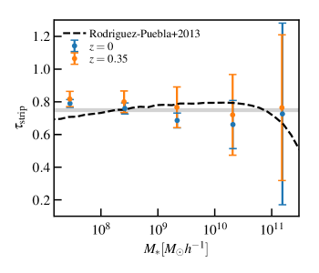
Figure 5: Stripping factor $\tau_{\mathrm{strip}}$ as a function of the mean stellar mass in each bin at $z=0$ (blue), and at $z=0.35$ (orange). The grey line represents the mean value, and the dashed line is the stripping factor computed using the SHMR from Rodríguez-Puebla et al. (2013).

4 Evolution since the time of accretion

In this section, we investigate which mechanisms drive this shift of the SHMR towards lower halo masses for subhaloes. Is it an evolution of the dark matter mass at fixed stellar mass, completely dominated by tidal stripping? Or is there a contribution from ongoing star formation? How does the tidal stripping and star formation quenching timescales compare? Is there a significant contribution from mergers? To start answering these questions we will follow the evolution of subhalo properties from the time of accretion to present time.

We choose again the three most massive haloes of Illustris-1 (with $M_{\rm h}>10^{14}\,h^{-1}{\rm M}_{\sun}$) as cluster-like haloes, and we examine the evolution of their subhaloes. We only select subhaloes with $M_{\mathrm{sub}}>10^{10}\,h^{-1}{\rm M}_{\sun}$, to guaranty a sufficient number of particles (i.e $N_{\rm{part}}>280$) to ensure that the subhaloes are reasonably resolved above the mass and force resolution of the simulation. We follow the evolution of the subhaloes with time, by extracting the main branch of their merger trees. We use the merger trees obtained with the SubLink algorithm as described in Sect. 2.1.

We need to define a time of reference, when the subhalo starts its accretion into the host halo. This accretion time $t_{\mathrm{acc}}$ is defined as the first time the halo enters the shell of radius $R_{\mathrm{acc}}$. We define the accretion radius as twice the virial radius of the host halo, $R_{\mathrm{acc}}=2\times R_{200}$. Indeed, the cluster environment extends far beyond the virial radius, and its influence on the infalling subhaloes can therefore start before they reach $R_{200}$. A more physically motivated choice for the accretion radius would be to use the splashback radius (More et al., 2015a; Busch & White, 2017; Baxter et al., 2017; Diemer et al., 2017), which is estimated by current measurements at around 1.5-2$\times R_{200}$, which motivates our choice of $R_{\rm{acc}}=2\times R_{200}$.

The subhaloes are then followed snapshot by snapshot after $t_{\mathrm{acc}}$. In addition, as the measurement of the subhalo mass across the snapshots can be noisy (Muldrew et al., 2011), we perform sigma-clipping in order to clean the mass evolution signal.

4.1 Evolution of the halo-centric distance

The first characteristic of interest is the distance between the subhalo and the centre of the host halo. The top panel of Fig. 6 shows the evolution of the cluster-centric distance normalized by the virial radius of the host at the time of accretion, as a function of time since accretion, for each of the three cluster-like haloes separately (each column corresponds to a different host). In each panel, the black curves represent the evolution for each subhalo independently, the thick red line indicates the median value at each time step, and the thin red lines highlight the evolution of the 16th and 84th percentiles.

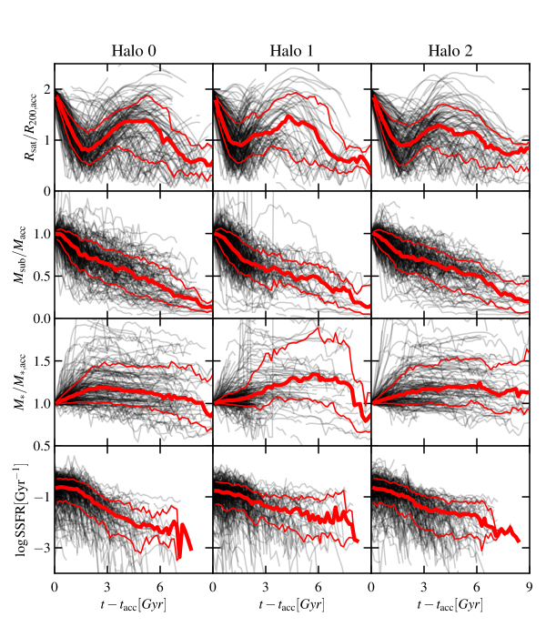
Figure 6: Evolution of subhalo properties as a function of time since accretion: halo-centric distance normalized by the host virial radius at accretion (top panel), subhalo dark matter mass normalized by the dark matter mass at accretion (second panel), stellar mass normalized by stellar mass at accretion (third panel), and specific star formation rate (SSFR) (bottom panel). Each column represents one of the cluster-like haloes. The black lines represent the evolution of each subhalo independently; the thick red line shows the median evolution, and the thin red lines mark the 16th and 84th percentiles.

As expected, the subhaloes are moving towards the centre of their hosts, and this overall infall motion has already started at $2\times R_{200}$ from the centre. It is therefore interesting to follow the properties of the subhaloes at this distance, as the majority of them will be accreted, and will end up in the central part of the cluster (Nipoti et al., 2018). One will note that some of them are already influenced by the cluster at such distance. In general, subhaloes are following spiraling orbits typically off-centered, leading them towards the centre of the cluster (Hayashi et al., 2003b; Hayashi et al., 2007).

We can also observe the first infall into the cluster, where the subhaloes pass close to the centre of the cluster. We measure for each host halo the time at which the average $R_{\rm{sat}}/R_{200,\rm{acc}}$ evolution reaches its first minimum: $t_{\rm{min}}=1.8\,\rm{Gyr}$ for Halo 0, $t_{\rm{min}}=1.5\,\rm{Gyr}$ for Halo 1, and $t_{\rm{min}}=1.7\,\rm{Gyr}$ for Halo 2. This first crossing has been discussed in some studies (see for example Jaffé et al., 2015) as the moment when the subhaloes are ram-pressure stripped from their gas. We will compare this timescale with the dark matter loss and star formation quenching timescales in the next sections.

4.2 Evolution of the dark matter mass

We now follow the evolution of the subhaloes dark matter content during infall. The top middle panel of Fig. 6 shows the time evolution of the mass of dark matter particles bound to the subhaloes normalized by the mass at accretion, $M_{\mathrm{sub}}/M_{\mathrm{acc}}$, as a function of time. We show the evolution for each subhalo and the median value at each time step.

Looking at the median evolution, the mass normalized by the mass at accretion shows a decrease over time, starting very soon after the subhaloes infall, at $2\times R_{200}$. We investigate that case more carefully, and discuss the mass-loss start time in Sect. 5. One can see two possible different regimes in the mass-loss, with the subhaloes losing matter more rapidly up to $t-t_{\mathrm{acc}}\sim 1.5\,\rm{Gyr}$. To check this trend, we fit a broken line to the mass evolution, to measure the two slopes of the evolution, $\alpha_{\rm{dm}}$ and $\beta_{\rm{dm}}$, as well as the time at which the slope changes, $t_{\rm{dm}}$. The function is defined as:

$$\frac{M_{\rm{sub}}}{M_{\rm{acc}}}(t)=\begin{cases}\alpha_{\rm{dm}}t+c_{\rm{dm}},&\mbox{if }t<t_{\rm{dm}}\\ \beta_{\rm{dm}}t+c^{\prime}_{\rm{dm}},&\mbox{if }t>t_{\rm{dm}}\end{cases}$$ (3)

, where $c^{\prime}=(\alpha_{\rm{dm}}-\beta_{\rm{dm}})t_{\rm{dm}}+c_{\rm{dm}}$. This is shown in the top panel of Fig. 7. We perform the fit on the median evolution over the subhaloes from the three host haloes. The best fit parameters are presented in Table 5.

The best fit evolution shows a slope change at $t_{\rm{DM}}=(1.72\pm 0.04)\,\rm{Gyr}$: on average subhaloes appear to lose their mass faster during their first infall, with a rate of $\sim 20\%$ of their mass at accretion per Gyr. The mass loss then slows down to a rate of $\sim 6\%$ of their mass at accretion per Gyr. As shown in previous studies (eg. Diemand et al., 2007), the subhaloes lose most of their mass at their successive passages at the pericenter, with a relatively larger fraction at the first passage.

As a comparison we compute a simple analytical model for the subhalo mass loss by tidal stripping. At each time step, the total mass that is gravitationally bound to the subhalo can be defined as being enclosed in the tidal radius, $r_{\rm t}$. Beyond this radius, matter is disrupted by the tidal forces of the host halo:

$$F_{\rm T}=-\frac{\rm d}{\mathrm{d}R_{\rm sat}}\left(\frac{GM_{\rm{host}}(R_{\rm{sat}})}{R_{\rm{sat}}^{2}}\right)r_{\rm t}\ ,$$ (4)

as they are stronger than the subhalo self-gravity:

$$F_{\rm G}=\frac{GM_{\rm{sub}}(r_{\rm t})}{r_{\rm t}^{2}}\ ,$$ (5)

, where $G$ is the gravitational constant. For each subhalo, and at each time step, we compute the value of the tidal radius by solving $F_{\rm T}=F_{\rm G}$, assuming that the (sub)haloes follow a Navarro-Frenk-White density profile (NFW, Navarro et al., 1996), to compute the mass. The subhalo mass is then defined as the NFW mass truncated at $r_{\rm t}$. The top panel of Fig. 7 shows as a dotted line the evolution of this theoretical value normalized by mass at accretion, and averaged over all the subhaloes of the three hosts.

The mass loss predicted by this simple analytical model is in very good agreement with the simulation during the first infall, i.e up to $\sim 2-3\,\rm{Gyr}$. However, after that it underestimates the mass loss. This is to be expected with such a simple model, as for instance it does not take into account the possible reorganization of the mass within the subhalo but considers that it keeps following a NFW mass distribution with an abrupt truncation at the tidal radius. Collisions between satellites might also play a role in the mass evolution, and are not included in such a simple model (Tormen et al., 1998).

In the top panel of Fig. 7, we also show the exponential mass loss from eq. (10) in Giocoli et al. (2008). Giocoli et al. (2008) adopt a different definition for the accretion time, namely the time when the subhalo crosses the virial radius of the host for the last time, which corresponds in our case to $t-t_{\rm{acc}}\sim 6\,\rm{Gyr}$ (see top panel of Fig. 6). We also let the parameter $\tau_{0}$ from their equation to vary, as subhaloes survive longer in simulations that include baryons. It appears indeed that the model from Giocoli et al. (2008) describes quite well the evolution that we measure after $t-t_{\rm{acc}}=6\,\rm{Gyr}$, when we fix $\tau_{0}=2.5-3\,\rm{Gyr}$.

Figure 6 shows that subhaloes that remain the longest in the host, up to $t=t_{\mathrm{acc}}+9\,\rm{Gyr}$, appear to lose $\sim 75\%$ of their mass. However, most of the subhaloes at $t=0$ have not started their infall into the cluster so long ago, and have therefore lost less than $75\%$ of their mass. To quantify this effect, we split the subhaloes into four samples according to their surviving mass at $z=0$, $f_{\rm{surv}}=M_{\rm{sub}}(z=0)/M_{\rm{sub}}(z_{\rm{acc}})$, and compute for each sample the mean time since accretion. As expected, we find that subhaloes with the lowest surviving mass ($f_{\rm{surv}}<0.25$) have spent more time in their host ($t_{0}-t_{\rm{acc}}\sim 8\,\rm{Gyr}$, where $t_{0}$ represents the present time), while subhaloes with a high surviving mass ($f_{\rm{surv}}>0.75$) have started their infall much more recently ($t_{0}-t_{\rm{acc}}\sim 2\,\rm{Gyr}$). Table 4 summarizes the values obtained for each sample considered.

$f_{\rm{surv}}$	$\langle f_{\rm{surv}}\rangle$	$\langle t_{0}-t_{\rm{acc}}\rangle$ (Gyr)
$[0,0.25]$	$0.15\pm 0.07$	$7.72\pm 2.11$
$[0.25,0.5]$	$0.40\pm 0.07$	$5.41\pm 2.10$
$[0.5,0.75]$	$0.62\pm 0.07$	$3.71\pm 1.80$
$[0.75,\infty]$	$0.94\pm 0.21$	$1.92\pm 1.41$

Table 4: Mean surviving mass, $f_{\rm{surv}}=M_{\rm{sub}}(z=0)/M_{\rm{sub}}(z_{\rm{acc}})$ at redshift $z=0$, and mean time since accretion, $t_{0}-t_{\rm{acc}}$, for subhaloes divided in bins of surviving mass. The error bars represent the standard deviation.

4.3 Stellar mass evolution

We now investigate whether the evolution of the stellar mass during infall could be partly responsible for the SHMR shift. Similar to the dark matter mass, we normalize the stellar mass at each epoch by the stellar mass at accretion; we present in the third panel of Fig. 6 the normalized stellar mass as a function of time for the three host haloes. The median stellar mass increases after the subhaloes cross $2\times R_{200}$, showing that on average galaxies still have ongoing star forming.

The median stellar mass then starts to stagnate, demonstrating that the star formation is slowing down after accretion. Similarly to the dark matter investigation, we measure the mean evolution over the three host haloes, and fit a broken line to it, defined as in equation 3. The median evolution is presented in the middle panel of Fig. 7, and the best fit parameters are listed in Table 5. The fit shows a transition between a regime where the stellar mass increases ($+6\%$ of the infall mass per Gyr), and a stagnation ($+0.3\%$ of the infall mass per Gyr) at $t_{*}=(2.98\pm 0.06)\,\rm{Gyr}$.

To see the transition more clearly, we show in the bottom panel of Fig. 6 the evolution with time of the Specific Star Formation Rate (SSFR), the ratio of star formation rate to stellar mass. Among the different definitions of the SFR in Illustris we chose the one compatible with our choice of stellar mass, i.e., the sum of the star formation rates of all gas cells within twice the stellar half mass radius of the subhalo. We fit the following function to the SSFR evolution:

$$\frac{M_{\rm{ssfr}}}{M_{\rm{acc}}}(t)=\begin{cases}\alpha_{\rm{ssfr}}t+c_{\rm{ssfr}},&\mbox{if }t<t_{\rm{ssfr}}\\ \beta_{\rm{ssfr}}t+c^{\prime}_{\rm{ssfr}},&\mbox{if }t_{\rm{ssfr}}<t<t^{\prime}_{\rm{ssfr}}\\ \gamma_{\rm{ssfr}}t+c^{\prime\prime}_{\rm{ssfr}},&\mbox{if }t>t^{\prime}_{\rm{ssfr}}.\end{cases}$$ (6)

where $c^{\prime}=(\alpha-\beta)t_{\rm{ssfr}}+c$ and $c^{\prime\prime}=(\beta-\gamma)t^{\prime}_{\rm{ssfr}}+(\alpha-\beta)t_{\rm{ssfr}}+c$.

The evolution of the SSFR shows a clear transition between galaxies that are on average star forming (SSFR $\sim 0.2\,\rm{Gyr}^{-1}$), and quenched (SSFR $\sim 0.01\,\rm{Gyr}^{-1}$), which happens mostly between $t_{\rm{ssfr}}=(1.21\pm 0.06)\,\rm{Gyr}^{-1}$, and $t^{\prime}_{\rm{ssfr}}=(3.32\pm 0.14)\,\rm{Gyr}^{-1}$. The three different phases are marked by a slope change in the SSFR evolution, with a slower evolution before $t_{\rm{ssfr}}$, and after $t^{\prime}_{\rm{ssfr}}$, than in the transition phase. This transition, happening a few Gyr after the beginning of accretion, is consistent with a slow-starvation delayed-quenching scenario of galaxy evolution in clusters (Tollet et al., 2017).

Figure 7: Median evolution of $M_{\mathrm{sub}}/M_{\mathrm{acc}}$ (top panel), $M_{\mathrm{*}}/M_{\mathrm{*,acc}}$ (middle panel), and SSFR (bottom panel), as a function of time (red line, with the error on the median as red filled surfaces), and the best fit evolution (black solid lines). The grey vertical line represents the time at which the mean evolution of the cluster-centric distance reaches its first minimum. The dotted line in the top panel represents the mass evolution from the dark matter stripping simple analytical model (see text for details), and the solid blue, orange and green lines correspond to the subhalo mass loss measured in Giocoli et al. (2008) with $\tau_{0}=2$, 2.5, and 3 Gyr respectively.

All haloes
	$M_{\rm{DM}}$	$M_{*}$	SSFR
$\alpha$	$-0.192\pm 0.005$	$0.058\pm 0.001$	$-0.086\pm 0.018$
$\beta$	$-0.064\pm 0.001$	$0.003\pm 0.001$	$-0.366\pm 0.011$
$\gamma$	–	–	$-0.142\pm 0.012$
$c$	$1.054\pm 0.004$	$1.002\pm 0.001$	$-0.674\pm 0.012$
$t$	$1.72\pm 0.05$	$2.98\pm 0.06$	$1.21\pm 0.06$
$t^{\prime}$	–	–	$3.32\pm 0.14$

Table 5: Best fit parameters of the evolution of the dark matter mass, stellar mass, and specific star formation rate (SSFR), as a function of time. The fits are performed on the median evolution over all the subhaloes of the three hosts.

In summary, looking at Fig. 7 it appears that during the first infall, subhaloes lose around 40% of their dark matter at accretion, but continue to form stars. Compared to the dark matter stripping, the star formation quenching is delayed, and only starts when the subhaloes get closer to the centre of the cluster. We note that we perform the fits presented in Fig. 7 and Table 5 only up to $t-t_{\rm{acc}}=6\,\rm{Gyr}$: the small quantity of remaining subhaloes after that time makes the signal much noisier. This also corresponds to the time scale at which, on average, subhaloes cross the host halo virial radius, where the influence of the host potential becomes much stronger.

In all our Figures so far, all mass evolution tracks are shown normalized by the mass at accretion. To highlight the relative importance of the dark matter and stellar mass loss, we show in Fig. 8 the evolution of the dark matter mass (blue solid line) and the stellar mass (orange dashed line), normalized by the total mass at accretion. This shows that the total mass evolution is dominated by the subhalo mass loss. It accounts for up to $90\%$ of the mass at accretion, while the stellar mass increase represents only $\sim 2\%$ of the total mass at accretion. However, due to these two effects, the proportion of stellar and dark matter changes drastically during accretion: the ratio of stellar to dark matter mass goes from 0.03 to 0.3 during that time (black dotted line in Fig. 8).

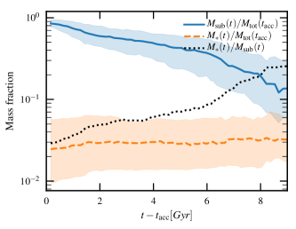
Figure 8: Evolution since the time of accretion of the dark matter (solid blue), and the stellar mass (dashed orange), normalized by the total mass at accretion. The solid and dashed lines represent the median evolution. The filled surfaces show the $68\%$ credible interval. The evolution of the stellar to subhalo mass ratio is represented as the black dotted line.

5 Evolution of mass vs $R_{\mathrm{sat}}$

To have a better representation of the relation between the quenching/stripping, and the trajectory of the subhaloes, we look at the evolution of the dark matter and stellar mass, as well as the SSFR, as a function of distance to the cluster centre. We keep the same subhalo selection as in Sect. 4.

Starting with the dark matter mass, the top panel of Fig. 9 shows, at each time step starting at their crossing of $2\times R_{200}$, the position of each subhalo on the $R_{\mathrm{sat}}-M_{\mathrm{sub}}/M_{\mathrm{acc}}$ plane. We also show the median value for all subhaloes at each time step as black dots, with error bars corresponding to the standard error. The dark matter mass appears to remain constant on average until subhaloes reach $\sim 1.5\times R_{\rm{vir}}$. This would indicate that subhaloes only start to be affected by their host when they cross some physical boundary of the halo. Such a physical boundary is now often considered to be the splashback radius, which is defined as the radius at which accreted matter reaches its first orbital apocenter after turnaround (More et al., 2015b, 2016; Busch & White, 2017; Baxter et al., 2017; Diemer et al., 2017). It has been measured to be located at $\sim$ 1-2$\times R_{\rm{vir}}$, which is consistent with what we observe.

The subhaloes then progressively lose their dark matter as they sink towards the centre of the host. Looking at the mean evolution, $\sim 30\%$ of the dark matter mass is stripped at the first pericentre, $\sim 50\%$ after the first orbit, and up to $80\%$ for subhaloes that spend $8-9\,\rm{Gyr}$ in their host.

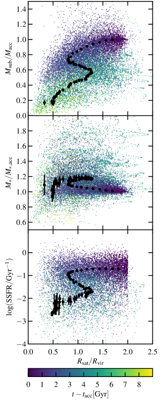
Figure 9: Position of the subhaloes on the $R_{\mathrm{sat}}-M_{\mathrm{sub}}/M_{\mathrm{acc}}$ (top panel), $R_{\mathrm{sat}}-M_{*}/M_{*,\mathrm{acc}}$ (middle panel), and $R_{\mathrm{sat}}-SSFR$ plane (bottom panel) at each time step, starting when they are accreted at $2\times R_{200}$. The color of each point represents the time since accretion. The black dots represent the median values at each time step.

We now look at the evolution of the stellar content of the subhaloes. The middle panel of Fig. 9 shows the evolution of the stellar mass as a function of the distance to the centre of the host. The bottom panel of Fig. 9 shows the evolution of the SSFR. This representation demonstrates more clearly how the delay in star formation quenching relates to accretion in the host. On average, the satellite galaxies continue to form stars during the first infall (increase in $M_{*}$, SSFR constant). The quenching process starts after the first passage at the pericentre.

In Smith et al. (2016), the authors study the stripping of stellar and dark matter in galaxies during their infall into simulated clusters, and found that $18\%$ of the galaxies were undergoing important star formation during accretion, with an increase in stellar mass higher than $15\%$. We test the influence of strongly star forming galaxies by removing all galaxies that increase their stellar mass by more that $50\%$ during their infall, which represent $10\%$ of the total number of satellite galaxies in our sample. Without them, the slope of the mean stellar mass increase before the first passage at the pericentre is only slightly modified (they reach $108\%$ of their initial stellar mass, instead of $109\%$ for the full sample). However, the sharp increase just after the pericentre passage is dampened (the maximum stellar mass is $114\%$ of the initial mass, compared to $120\%$ for the full sample at the same moment). This could suggest that a small fraction of galaxies experience a violent star formation burst, close to their passage at the pericentre: observations of such star formation bursts in infalling galaxies have been reported for example in Gavazzi et al. (2003), who argue that it is caused by enhanced ram-pressure during a high velocity infall.

6 Summary and discussion

In this paper, we present a study of the evolution of satellite galaxies during their infall into the three most massive haloes of Illustris-1. We first measure the SHMR for central, and satellite galaxies separately, and give a fitting function for each case. We find that the SHMR for satellite galaxies is shifted towards lower halo mass compared to central galaxies. We find no dependence of this shift on the galaxy stellar mass, with a mean value $<\tau_{\rm{strip}}>=0.75$, where $\tau_{\rm{strip}}$ is defined as the shift in subhalo mass at a given stellar mass (see equation 2). This stripping factor is also in good agreement with the SHMR measured for central and satellite galaxies in Rodríguez-Puebla et al. (2013).

We note that both for haloes and subhaloes, the SHMR we measure differs at both mass ends from what is measured with abundance matching (Moster et al., 2013; Rodríguez-Puebla et al., 2013). There is in particular an excess of massive galaxies that could be explained by an underestimation of AGN feedback in the simulation that fails to properly reduce star formation in massive haloes. It would therefore be interesting to follow up on this work using the IllustrisTNG simulation, which includes a new modeling of both stellar and AGN feedback. In addition, the evolution of the SHMR that we measure between $z=0$ and $z=0.35$ is weaker than what was predicted in Moster et al. (2013). The larger volume of the IllustrisTNG-300 simulation set could be useful to study the redshift evolution of the SHMR for central and satellite galaxies in detail.

To understand which mechanisms drive the shift of the SHMR for satellite galaxies, we look at the time evolution of the stellar and dark matter mass of the subhaloes during their infall. We find that subhaloes lose a significant amount of their mass after their accretion by the cluster (at a distance smaller than $\sim 1.5\times R_{200}$). As predicted by analytical models of tidal stripping, mass loss happens the fastest during the pericentric passages, with an average of $30\%$ of the initial mass lost during the first passage at the pericentre. This is in good agreement with the analysis presented in Rhee et al. (2017), where they found that subhaloes lose $20-30\%$ of their initial mass during the first pericentric passage, the rest of the mass loss being attributed to subsequent passages at the pericentre, as well as to close encounters with other subhaloes. As an additional check, we bin subhaloes by their mass at infall, and measure the median evolution in each bin: from their first passage in the cluster, the most massive ones are found on tighter orbits, and lose their dark matter more quickly (see also Xie & Gao, 2015). We find that during the first infall, less massive galaxies ($\log M_{*}<10$) lose around 25% of their initial mass, while the most massive galaxies ($\log M_{*}>10$) around 40%.

The quenching of star formation is delayed compared to dark matter stripping, and on average, galaxies stop forming new stars after their first passage within the host core. The median evolution of the SSFR suggests a slow quenching mechanism, with a quenching time $t_{\rm{Q}}\sim 2\,\rm{Gyr}$. This value is in very good agreement with the time scale estimated for instance in Haines et al. (2015), and suggests that the dominant quenching mechanism is galaxy starvation. To check a potential mass dependance of the star formation rate evolution, we split the galaxies by their stellar mass at infall, and measure the median evolution in each bin. We find two weak stellar mass dependencies: (i) galaxies in the lower mass bins ($7<\log M_{*}<9$) have a slightly steeper evolution than higher mass galaxies ($9<\log M_{*}<11$), leading to shorter quenching times ($t_{\rm{Q}}\sim 1.8\,\rm{Gyr}$ for low mass, and $t_{\rm{Q}}\sim 2.5\,\rm{Gyr}$ for higher mass); (ii) galaxies in the highest mass bin ($\log M_{*}>11$) are already mostly quenched at infall. The latter effect could point towards an important role of pre-processing for high mass galaxies. However, this result should be taken with care as our highest mass bin contains only $\sim 30$ objects. Around 8 Gyr after accretion, the average stellar mass of satellite galaxies starts to decrease as well. This could imply that stellar mass starts to be stripped as well when subhaloes only have $\sim 30-40\%$ of their remaining dark matter mass. This could also be an artifact due to the small number of galaxies that have spent more than $7\,\rm{Gyr}$ in their hosts. However, this is in very good agreement with the evolution measured in Smith et al. (2016), where the stellar mass starts decreasing only after $70\%$ of the dark matter mass is stripped.

We summarize the measured evolution of the SHMR of satellite galaxies in Fig. 10. The evolution can be divided into three phases. During the first one, which corresponds roughly to the first infall, the galaxies lose on average $\sim 30\%$ of their dark matter mass at accretion, and continue to form stars, reaching $\sim 120\%$ of their initial mass (red arrows in Fig. 10). Star formation is then quenched, and the subhaloes continue to lose mass while the stellar mass remains constant (green arrows). Finally, when only $30\%$ of the initial dark matter mass remains, the average stellar mass starts to decrease as well (blue arrows). We note that the evolution represented by the arrows seems to predict a larger evolution of the SHMR than what we measured (dashed line): this is simply due to the fact that not all subhaloes follow this evolutionary path until the end, but are distributed along the way. We note that due to the limited size of the Illustris-1 simulation we did not investigate the dependence of the SHMR evolution on the host mass, but this could be tested with IllustrisTNG-300, which contains haloes with masses up to $10^{15}M_{\sun}$.

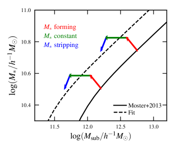
Figure 10: Summary of the subhalo SHMR evolution. The black solid line represents the SHMR for central galaxies at $z=0$ from Moster et al. (2013), and the dashed line the fit from Sect. 3. The arrows show the three different phases of the evolution: dark matter stripping + star formation in red, dark matter stripping only in green, and dark + stellar matter stripping in blue.

Although studies of simulations such as the one presented here allow to disentangle the evolution of the dark component from the stellar one, it is much more difficult in observational works. The only observable that can potentially be obtained is the stripping factor $\tau_{\rm strip}$ which includes both the stripping of dark matter, and the formation or stripping of stellar matter. However, if the true evolution is similar to what simulations predict, dark matter stripping should be the main contributor to the shift of the SHMR. Figure 10 shows that the amplitude of the subhalo mass evolution is $\sim 0.6$ dex, while it is only 0.1 dex for the stellar mass. In any case, the stripping of subhaloes (or SHMR shift) has not yet been measured with high confidence in observations. For instance, weak gravitational lensing allows to statistically measure the total mass of subhaloes, with a precision that is proportional to the area, and the depth of the available observations. The advent of large galaxy surveys such as DES or Euclid in the future, could therefore allow to put stronger observational constrains on the SHMR shift in clusters.

Another aspect that remains observationally challenging is to estimate the stage of accretion of galaxies in clusters, and even simply their membership. A commonly used proxy is the projected distance to the cluster centre, which is on average indeed correlated with the time since accretion but adds noise coming from the shapes of the individual orbits and from line-of-sight projections. Future data coming from upcoming ground- and space-based facilities will allow a better characterization of cluster membership and environment. It will also provide an increase of the statistical sample of several orders of magnitude (Sartoris et al., 2016), and will allow us to shed more light on the dark and visible properties of satellite galaxies in clusters.

Appendix A Corner plots

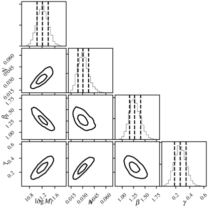
Figure 11: Joint 2-dimensional and marginalized 1-dimensional posterior probability distributions for the SHMR parameters $M_{1}$, $N$, $\beta$, and $\gamma$ fitted to central galaxies at $z=0$.

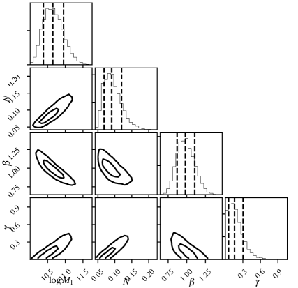
Figure 12: Same as Fig. 11 but for satellite galaxies.

References

- Acreman et al. (2003) Acreman D. M., Stevens I. R., Ponman T. J., Sakelliou I., 2003, MNRAS, 341, 1333
- Bahé & McCarthy (2015) Bahé Y. M., McCarthy I. G., 2015, MNRAS, 447, 969
- Bahé et al. (2017) Bahé Y. M., et al., 2017, MNRAS, 470, 4186
- Baxter et al. (2017) Baxter E., et al., 2017, ApJ, 841, 18
- Binney & Tremaine (2008) Binney J., Tremaine S., 2008, Galactic Dynamics: Second Edition. Princeton University Press
- Bluck et al. (2016) Bluck A. F. L., et al., 2016, MNRAS, 462, 2559
- Bonafede et al. (2011) Bonafede A., Dolag K., Stasyszyn F., Murante G., Borgani S., 2011, MNRAS, 418, 2234
- Boselli et al. (2016) Boselli A., et al., 2016, A&A, 596, A11
- Buck et al. (2019) Buck T., Macciò A. V., Dutton A. A., Obreja A., Frings J., 2019, MNRAS, 483, 1314
- Busch & White (2017) Busch P., White S. D. M., 2017, MNRAS, 470, 4767
- Butcher & Oemler (1978) Butcher H., Oemler Jr. A., 1978, ApJ, 226, 559
- Conroy et al. (007b) Conroy C., Wechsler R. H., Kravtsov A. V., 2007b, ApJ, 668, 826
- De Boni et al. (2018) De Boni C., Böhringer H., Chon G., Dolag K., 2018, MNRAS, 478, 2086
- De Lucia & Blaizot (2007) De Lucia G., Blaizot J., 2007, MNRAS, 375, 2
- De Lucia et al. (2004) De Lucia G., Kauffmann G., Springel V., White S. D. M., Lanzoni B., Stoehr F., Tormen G., Yoshida N., 2004, MNRAS, 348, 333
- De Lucia et al. (2012) De Lucia G., Weinmann S., Poggianti B. M., Aragón-Salamanca A., Zaritsky D., 2012, MNRAS, 423, 1277
- Diemand et al. (2007) Diemand J., Kuhlen M., Madau P., 2007, ApJ, 667, 859
- Diemer et al. (2017) Diemer B., Mansfield P., Kravtsov A. V., More S., 2017, ApJ, 843, 140
- Dolag et al. (2009) Dolag K., Borgani S., Murante G., Springel V., 2009, MNRAS, 399, 497
- Dressler (1980) Dressler A., 1980, ApJ, 236, 351
- Foreman-Mackey et al. (2013) Foreman-Mackey D., Hogg D. W., Lang D., Goodman J., 2013, PASP, 125, 306
- Gan et al. (2010) Gan J., Kang X., van den Bosch F. C., Hou J., 2010, MNRAS, 408, 2201
- Gao et al. (2004) Gao L., White S. D. M., Jenkins A., Stoehr F., Springel V., 2004, MNRAS, 355, 819
- Gavazzi et al. (2003) Gavazzi G., Cortese L., Boselli A., Iglesias-Paramo J., Vílchez J. M., Carrasco L., 2003, ApJ, 597, 210
- Genel et al. (2014) Genel S., et al., 2014, MNRAS, 445, 175
- George et al. (2013) George M. R., Ma C.-P., Bundy K., Leauthaud A., Tinker J., Wechsler R. H., Finoguenov A., Vulcani B., 2013, ApJ, 770, 113
- Ghigna et al. (1998) Ghigna S., Moore B., Governato F., Lake G., Quinn T., Stadel J., 1998, MNRAS, 300, 146
- Giocoli et al. (2007) Giocoli C., Moreno J., Sheth R. K., Tormen G., 2007, MNRAS, 376, 977
- Giocoli et al. (2008) Giocoli C., Tormen G., van den Bosch F. C., 2008, MNRAS, 386, 2135
- Giocoli et al. (2010) Giocoli C., Tormen G., Sheth R. K., van den Bosch F. C., 2010, MNRAS, 404, 502
- Giocoli et al. (2012) Giocoli C., Tormen G., Sheth R. K., 2012, MNRAS, 422, 185
- Giocoli et al. (2013) Giocoli C., Marulli F., Baldi M., Moscardini L., Metcalf R. B., 2013, MNRAS, 434, 2982
- Gunn & Gott (1972) Gunn J. E., Gott III J. R., 1972, ApJ, 176, 1
- Guo et al. (2010) Guo Q., White S., Li C., Boylan-Kolchin M., 2010, MNRAS, 404, 1111
- Guo et al. (2015) Guo Q., et al., 2015, Monthly Notices of the Royal Astronomical Society, 461
- Haines et al. (2015) Haines C. P., et al., 2015, ApJ, 806, 101
- Han et al. (2016) Han J., Cole S., Frenk C. S., Jing Y., 2016, MNRAS, 457, 1208
- Hayashi et al. (2003a) Hayashi E., Navarro J. F., Taylor J. E., Stadel J., Quinn T., 2003a, ApJ, 584, 541
- Hayashi et al. (2003b) Hayashi E., Navarro J. F., Taylor J. E., Stadel J., Quinn T., 2003b, ApJ, 584, 541
- Hayashi et al. (2007) Hayashi E., Navarro J. F., Springel V., 2007, MNRAS, 377, 50
- Hinshaw et al. (2013) Hinshaw G., et al., 2013, ApJS, 208, 19
- Hiroshima et al. (2018) Hiroshima N., Ando S., Ishiyama T., 2018, Phys.Rev.D, 97, 123002
- Jaffé et al. (2015) Jaffé Y. L., Smith R., Candlish G. N., Poggianti B. M., Sheen Y.-K., Verheijen M. A. W., 2015, MNRAS, 448, 1715
- Kauffmann et al. (1993) Kauffmann G., White S. D. M., Guiderdoni B., 1993, MNRAS, 264, 201
- Klypin et al. (2011) Klypin A. A., Trujillo-Gomez S., Primack J., 2011, ApJ, 740, 102
- Klypin et al. (2016) Klypin A., Yepes G., Gottlöber S., Prada F., Heß S., 2016, MNRAS, 457, 4340
- Kravtsov et al. (2004) Kravtsov A. V., Gnedin O. Y., Klypin A. A., 2004, ApJ, 609, 482
- Lacey & Cole (1993) Lacey C., Cole S., 1993, MNRAS, 262, 627
- Lacey & Cole (1994) Lacey C., Cole S., 1994, MNRAS, 271, 676
- Li et al. (2016) Li R., et al., 2016, MNRAS, 458, 2573
- Limousin et al. (2007) Limousin M., Kneib J. P., Bardeau S., Natarajan P., Czoske O., Smail I., Ebeling H., Smith G. P., 2007, A&A, 461, 881
- Lotz et al. (2018) Lotz M., Remus R.-S., Dolag K., Biviano A., Burkert A., 2018, preprint, (arXiv:1810.02382)
- Mamon (2000) Mamon G. A., 2000, in Combes F., Mamon G. A., Charmandaris V., eds, Astronomical Society of the Pacific Conference Series Vol. 197, Dynamics of Galaxies: from the Early Universe to the Present. p. 377 (arXiv:astro-ph/9911333)
- Martinović & Micic (2017) Martinović N., Micic M., 2017, preprint, (arXiv:1706.04022)
- Merritt (1983) Merritt D., 1983, ApJ, 264, 24
- Merritt (1985) Merritt D., 1985, ApJ, 289, 18
- Moore et al. (1996) Moore B., Katz N., Lake G., Dressler A., Oemler A., 1996, Nature, 379, 613
- Moore et al. (1998) Moore B., Lake G., Katz N., 1998, ApJ, 495, 139
- More et al. (2015a) More S., Miyatake H., Mandelbaum R., Takada M., Spergel D. N., Brownstein J. R., Schneider D. P., 2015a, ApJ, 806, 2
- More et al. (2015b) More S., Diemer B., Kravtsov A. V., 2015b, ApJ, 810, 36
- More et al. (2016) More S., et al., 2016, ApJ, 825, 39
- Moster et al. (2013) Moster B. P., Naab T., White S. D. M., 2013, MNRAS, 428, 3121
- Muldrew et al. (2011) Muldrew S. I., Pearce F. R., Power C., 2011, MNRAS, 410, 2617
- Munshi et al. (2013) Munshi F., et al., 2013, ApJ, 766, 56
- Nagai & Kravtsov (2005) Nagai D., Kravtsov A. V., 2005, ApJ, 618, 557
- Natarajan et al. (2009) Natarajan P., Kneib J.-P., Smail I., Treu T., Ellis R., Moran S., Limousin M., Czoske O., 2009, ApJ, 693, 970
- Navarro et al. (1996) Navarro J. F., Frenk C. S., White S. D. M., 1996, ApJ, 462, 563
- Niemiec et al. (2017) Niemiec A., et al., 2017, MNRAS, 471, 1153
- Nipoti et al. (2018) Nipoti C., Giocoli C., Despali G., 2018, MNRAS, 476, 705
- Oemler (1974) Oemler Jr. A., 1974, ApJ, 194, 1
- Rhee et al. (2017) Rhee J., Smith R., Choi H., Yi S. K., Jaffé Y., Candlish G., Sánchez-Jánssen R., 2017, ApJ, 843, 128
- Rodriguez-Gomez et al. (2015) Rodriguez-Gomez V., et al., 2015, MNRAS, 449, 49
- Rodríguez-Puebla et al. (2012) Rodríguez-Puebla A., Drory N., Avila-Reese V., 2012, ApJ, 756, 2
- Rodríguez-Puebla et al. (2013) Rodríguez-Puebla A., Avila-Reese V., Drory N., 2013, ApJ, 767, 92
- Rozo & Rykoff (2014) Rozo E., Rykoff E. S., 2014, ApJ, 783, 80
- Rykoff et al. (2014) Rykoff E. S., et al., 2014, ApJ, 785, 104
- Sartoris et al. (2016) Sartoris B., et al., 2016, MNRAS, 459, 1764
- Sawala et al. (2013) Sawala T., Frenk C. S., Crain R. A., Jenkins A., Schaye J., Theuns T., Zavala J., 2013, MNRAS, 431, 1366
- Schaye et al. (2015) Schaye J., et al., 2015, MNRAS, 446, 521
- Sifón et al. (2015) Sifón C., et al., 2015, MNRAS, 454, 3938
- Sifón et al. (2018) Sifón C., Herbonnet R., Hoekstra H., van der Burg R. F. J., Viola M., 2018, MNRAS, 478, 1244
- Smith et al. (2016) Smith R., Choi H., Lee J., Rhee J., Sanchez-Janssen R., Yi S. K., 2016, ApJ, 833, 109
- Snyder et al. (2015) Snyder G. F., et al., 2015, MNRAS, 454, 1886
- Somerville et al. (2008) Somerville R. S., Hopkins P. F., Cox T. J., Robertson B. E., Hernquist L., 2008, MNRAS, 391, 481
- Springel (2010a) Springel V., 2010a, MNRAS, 401, 791
- Springel (2010b) Springel V., 2010b, MNRAS, 401, 791
- Springel et al. (2001) Springel V., White S. D. M., Tormen G., Kauffmann G., 2001, MNRAS, 328, 726
- Springel et al. (2005) Springel V., et al., 2005, Nature, 435, 629
- Terrazas et al. (2016) Terrazas B. A., Bell E. F., Henriques B. M. B., White S. D. M., Cattaneo A., Woo J., 2016, ApJ, 830, L12
- Tollet et al. (2017) Tollet É., Cattaneo A., Mamon G. A., Moutard T., van den Bosch F. C., 2017, MNRAS, 471, 4170
- Tormen (1998) Tormen G., 1998, MNRAS, 297, 648
- Tormen et al. (1998) Tormen G., Diaferio A., Syer D., 1998, MNRAS, 299, 728
- Tormen et al. (2004) Tormen G., Moscardini L., Yoshida N., 2004, MNRAS, 350, 1397
- Vale & Ostriker (2004) Vale A., Ostriker J. P., 2004, MNRAS, 353, 189
- Vogelsberger et al. (2014a) Vogelsberger M., et al., 2014a, MNRAS, 444, 1518
- Vogelsberger et al. (2014b) Vogelsberger M., et al., 2014b, Nature, 509, 177
- Wellons et al. (2015) Wellons S., et al., 2015, MNRAS, 449, 361
- White & Frenk (1991) White S. D. M., Frenk C. S., 1991, ApJ, 379, 52
- Wolf et al. (2009) Wolf C., et al., 2009, MNRAS, 393, 1302
- Xie & Gao (2015) Xie L., Gao L., 2015, MNRAS, 454, 1697
- Xu et al. (2017) Xu D., Springel V., Sluse D., Schneider P., Sonnenfeld A., Nelson D., Vogelsberger M., Hernquist L., 2017, MNRAS, 469, 1824
- Zinger et al. (2016) Zinger E., Dekel A., Kravtsov A. V., Nagai D., 2016, arXiv e-prints,
- van den Bosch et al. (2005) van den Bosch F. C., Tormen G., Giocoli C., 2005, MNRAS, 359, 1029